Discrete scattering by a pair of parallel defects

Abstract

Scattering of a time harmonic anti-plane shear wave due to either a pair of crack tips or a pair of rigid constraint tips on square lattice is considered. The two problems correspond to the so called zero-offset case of scattering due to a pair of identical Sommerfeld screens. The peculiar structural symmetry allows the reduction of coupled equations to two scalar Wiener–Hopf equations and a total of four geometrically reduced problems on lattice half-plane. Exact solution of each problem for incidence from the bulk lattice, as well as from an associated lattice waveguide, is constructed. A suitable superposition of the four expressions is used to construct the solution of the main problem. The discrete paradigm involving the wave mode incident from the waveguide is relevant for modern applications where an investigation of mechanisms of electronic and thermal transport at nanoscale remains an interesting problem.

1 Introduction

A square lattice based analogue of a canonical problem in scattering theory [cheney1951diffraction, Jones1, meister1996factorization, thompson2005mode] is discussed: a time harmonic lattice wave is incident upon a pair of semi-infinite parallel rows with either Neumann or Dirichlet condition. It is instructive to recall that, within the well established continuum framework, the scattering problem finds relevance in electro-magnetism, acoustics, and allied subjects [williams_1954, jones_1952, jull1973aperture, johansen1965radiation, crease1958propagation, Abrahams1, james1979double, kapoulitsas1984propagation, michaeli1985new, michaeli1996asymptotic], as well as from the viewpoint of geometric and asymptotic approximations [bowman1970comparison, BoersmaLee, MenendezLee]. Strikingly, in the presence of an offset between the edges, so called staggered case, the scattering problem is difficult to solve [jones1973double, Jones3planes, Abrahams0] owing to the complexity of matrix Wiener–Hopf (WH) factorization [Heinslim, MeisterRottbrand, Meistersys1, Meistersys2, daniele1984solution, AbrahamsExpo]. On the other hand, when the edges are not staggered an exact solution is well known [Heins1, Heins2]; this also plays a crucial role for solving the problem with small stagger in light of an asymptotic technique [Mishuris2014].

Within the discrete framework, the two structures, that is, a pair of parallel cracks (Neumann condition) or a pair of rigid constraints (Dirichlet condition), can be construed as the two dimensional formulation of a three dimensional structure with a pair of parallel atomically thin cracks or rigid inclusions. The latter can be envisaged for a crystal lattice having a symmetry that allows square sub-lattice planes and at the same time admits an out-of-plane displacement relative to such sub-lattices. Both cracks or rigid inclusions can extend indefinitely in one direction and are spaced apart by certain multiples of the lattice parameter. In this paper, the incident lattice wave field as well as the scattered wave field is time harmonic with the the same frequency. Moreover, it is assumed that there is a very small amount of damping present in the medium which results into a complex valued frequency with vanishingly small but positive imaginary part. The angle of incidence of the incident wave and the (real part of) incident wave frequency can be arbitrary chosen according to the passband of the considered square lattice structure [Brillouin].

Figure 1: Square lattice attached to a single lead created by breaking bonds in a pair of semi-infinite rows.

The present paper provides an exact solution of the stated discrete scattering problem and develops a far-field approximation for the incidence from the bulk lattice as well as for the incidence from the lattice waveguide formed between defects. Analytical expressions are also provided for certain physically relevant quantities, such the crack opening displacement, namely, the foremost (broken) bond length in any of the two cracks, and the displacement of a site adjacent to the rigid constraint tip. In the scenario presented so far, the scattering problem attended in the paper involves a purely mechanical framework, however, there is a quantum-mechanical analogue as well within the tight binding approximation for the electronic wave function (see §7.3 of [Bls9hx] for honeycomb lattice). The mathematical connection between a specific lattice wave (phonon) based expression [Bls9s] and that for the electronic wave has been spotted in this context [Bls5c_tube, Bls5c_tube_media]. In the mechanical framework, a significant scientific problem of current interest concerns the nature of energy transport in structures at small scales [Cahill1]. In this regime, the transport is typically defined in terms of reflection and transmission, i.e., by so called the Landauer viewpoint [Landauer1957, Landauer1992, Imry1999]. The problem tackled in the paper can be also viewed as a lattice attached to a single lead (the waveguide) which is created by breaking bonds in a pair of semi-infinite rows. The analysis of the energy flux relative to the waveguide, thus lying between the semi-infinite defects, is a derived entity based on the exact solution presented in this paper (schematically shown in Fig. 1); the relevant analysis and details shall appear elsewhere. Additionally, the non-zero offset case remains a difficult issue even in the discrete case [GMthesis], this is not analyzed in this paper.

2 Lattice model

An infinite square lattice, denoted by ${{\mathfrak{S}}}$, as a mechanical structure undergoing anti-plane shear motion, is considered. The lattice consists of identical particles, with in-plane spacing $\mathrm{b}$, each having unit mass and interacting with only its four nearest neighbours through bonds with a spring constant ${1}/{\mathrm{b}^{2}}$ (see [Bls0] for peculiar choice of scales). A time harmonic lattice wave is assumed to be incident on a pair of rigid constraints or cracks. A crack is modeled by assuming that the spring constant between the particles surrounding the crack is zero, while the rigid constraint is characterized by the vanishing of total displacement at each constrained site. For convenience, in this paper, sometimes a subscript ‘${{k}}$’ and ‘${{c}}$’ is used to represent an entity associated with case of cracks and rigid constraints, respectively.

Let ${{\Sigma}}_{{k}}$ (resp. ${{\Sigma}}_{{c}}$) denote the set of all lattice sites in ${{\mathfrak{S}}}$ associated with the crack-faces (resp. rigid constraints), that is precisely those sites which miss one nearest neighbor bond (resp. those sites whose displacement is restricted to be zero). Suppose ${N}$ is a positive integer (greater than $1$). Let ${\mathbb{Z}}$ denote the set of all integers. Let ${{\mathbb{Z}}^{2}}$ denote the set ${\mathbb{Z}}\times{\mathbb{Z}}$. Corresponding to a separation of $2{N}$ (resp. $2{N}-1$), i.e., for even (resp. odd) width ${N_{w}}$ of waveguide formed between both cracks,

Σ_k:={(x, y)∈Z^2: x≥0, y=-N, -N-1}∪{(x, y)∈Z^2: x≥0, y=N, N-1},
(resp. Σ’_k:={(x, y)∈Z^2: x≥0, y=-N+1,-N}∪{(x, y)∈Z^2: x≥0, y=N, N-1}). With separation $$2{N} 2{N}-1 {N_{w}}$$ (resp. ), i.e., even (resp. odd) waveguide within rigid constraints, Σ_c&:={(x, y)∈Z^2: (x, -N-1)∈Z^2: x≥0}∪{(x, y)∈Z^2: (x, +N)∈Z^2: x≥0},
(resp. Σ’_c:={(x, y)∈Z^2: (x, -N)∈Z^2: x≥0}∪{(x, y)∈Z^2: (x, +N)∈Z^2: x≥0}).

For convenience, the two different parities of the width ${N_{w}}$ are represented by a parity bit    (${{\,\gimel\,}}=1$ corresponding to the odd case and ${{\,\gimel\,}}=0$ for even). The sets ${{\Sigma}}_{{k}},{{\Sigma}}^{\prime}_{{k}},{{\Sigma}}_{{c}},{{\Sigma}}^{\prime}_{{c}},$ from (2.1) and (2.1), can be alternatively described as the broken bonds exist between ${\mathtt{y}}={N},{N}-1$ and ${\mathtt{y}}=-{N}+{{\,\gimel\,}},-{N}-1+{{\,\gimel\,}}$, while the rigid constraints are located at ${\mathtt{y}}={N}$ and ${\mathtt{y}}=-{N}-1+{{\,\gimel\,}}$. With ${\Sigma}$ representing either of ${{\Sigma}}_{{k}}$, ${{\Sigma}}^{\prime}_{{k}}$, ${{\Sigma}}_{{c}}$, ${{\Sigma}}^{\prime}_{{c}}$, the equation of motion at $({\mathtt{x}},{\mathtt{y}})\in{{{\mathbb{Z}}^{2}}}\setminus{\Sigma}$ is d2dt2u_x, y=1b2△u_x, y, where △u_x, y:=u_x+1, y+u_x-1, y+u_x, y+1+u_x, y-1-4u_x, y.

Remark 1

The equation of motion on sites located on the upper and lower face of a crack, respectively, is

$$\frac{d^{2}}{dt^{2}}{\mathtt{u}}_{{\mathtt{x}},{\mathtt{y}}}=\frac{1}{\mathrm{b}^{2}}({\mathtt{u}}_{{\mathtt{x}}+1,{\mathtt{y}}}+{\mathtt{u}}_{{\mathtt{x}}-1,{\mathtt{y}}}+{\mathtt{u}}_{{\mathtt{x}},{\mathtt{y}}+1}-3{\mathtt{u}}_{{\mathtt{x}},{\mathtt{y}}}),$$ (2.2a)

$$\frac{d^{2}}{dt^{2}}{\mathtt{u}}_{{\mathtt{x}},{\mathtt{y}}}=\frac{1}{\mathrm{b}^{2}}({\mathtt{u}}_{{\mathtt{x}}+1,{\mathtt{y}}}+{\mathtt{u}}_{{\mathtt{x}}-1,{\mathtt{y}}}+{\mathtt{u}}_{{\mathtt{x}},{\mathtt{y}}-1}-3{\mathtt{u}}_{{\mathtt{x}},{\mathtt{y}}}).$$ (2.2b)

Remark 2

The equation of motion on sites immediately above and below a rigid constraint, respectively, is

$$\frac{d^{2}}{dt^{2}}{\mathtt{u}}_{{\mathtt{x}},{\mathtt{y}}}=\frac{1}{\mathrm{b}^{2}}({\mathtt{u}}_{{\mathtt{x}}+1,{\mathtt{y}}}+{\mathtt{u}}_{{\mathtt{x}}-1,{\mathtt{y}}}+{\mathtt{u}}_{{\mathtt{x}},{\mathtt{y}}+1}-4{\mathtt{u}}_{{\mathtt{x}},{\mathtt{y}}}),$$ (2.3a)

$$\frac{d^{2}}{dt^{2}}{\mathtt{u}}_{{\mathtt{x}},{\mathtt{y}}}=\frac{1}{\mathrm{b}^{2}}({\mathtt{u}}_{{\mathtt{x}}+1,{\mathtt{y}}}+{\mathtt{u}}_{{\mathtt{x}}-1,{\mathtt{y}}}+{\mathtt{u}}_{{\mathtt{x}},{\mathtt{y}}-1}-4{\mathtt{u}}_{{\mathtt{x}},{\mathtt{y}}}).$$ (2.3b)

The equation of motion for the single site facing a semi-infinite rigid constraint is d2dt2u_x, y=1b2(u_x+1, y+u_x, y+1+u_x, y-1-4u_x, y), Indeed, for the sites on each rigid constraint $${\mathtt{u}}_{{\mathtt{x}},{\mathtt{y}}}=0$$.

In this paper, the considered structure admits two distinct kinds of incident waves: one type of incident wave is the bulk lattice wave that corresponds to the passband of the square lattice outside the waveguide formed by the two semi-infinite defects, while the second type of incident wave is the lattice waveguide mode that corresponds to the passband of the waveguide formed by the two semi-infinite defects. The role of type of incidence is emphasized by writing ‘incidence from the bulk lattice’ vis-a-vis ‘incidence from the waveguide’. Consider the former and let ${\mathtt{u}}^{\operatorname{i}B}$ describe the incident wave with frequency $\operatorname{\omega}$ and a lattice wave vector $({\upkappa}_{x},{\upkappa}_{y})$; specifically, u_x, y^iB:=Ae^iκ_x x+iκ_y y-iωt, where ${{\mathrm{A}}}\in{\mathbb{C}}$ is constant (${\mathbb{C}}$ denotes the set of complex numbers; ${z}\in{\mathbb{C}},$ ${z}={z}_{1}+i{z}_{2},{z}_{1}\in{\mathbb{R}},{z}_{2}\in{\mathbb{R}}$ with ${\mathbb{R}}$ as the set of real numbers). Following a traditional choice in diffraction theory [Bouwkamp, Noble], as a way to avoid the technical issues associated with nondecaying wavefronts, a vanishingly small amount of damping is introduced in the lattice model. This leads to a complex $\operatorname{\omega}$ with a vanishingly small but positive imaginary part.

Figure 2: Square lattice with a pair of semi-infinite (a) cracks and (b) rigid constraints. Illustration provides the contourplot of the total wavefield, obtained by numerical scheme (summarized in an Appendix of [Bls0]), in the presence of incident wave (2) (shown as thick white ray). Here ${\,\gimel\,}=1$ as ${N_{w}}$ is odd.

Throughout the paper, the factor, $e^{-i\operatorname{\omega}t}$, is suppressed. In the absence of damping, by virtue of (2.1) in intact lattice (${\mathtt{u}}={\mathtt{u}}^{\operatorname{i}B}$), the triplet ${\upomega}$ (${:=}\mathrm{b}\operatorname{\omega}$), ${\upkappa}_{x},$ and ${\upkappa}_{y}$ satisfies the dispersion relation ω^2 =4(sin^212κ_x+sin^212κ_y),   (κ_x, κ_y)∈[-π, π]^2, while the lattice wave (2) is diffracted by the pair of semi-infinite defects as illustrated by Fig. 2. With ${\upomega}={\upomega}_{1}+i{\upomega}_{2},{\upomega}_{2}>0$, it is easy to see that the wave number of the bulk incident lattice wave ${\mathtt{u}}^{\operatorname{i}B}$ (2) is also a complex number, i.e., ${\upkappa}={\upkappa}_{1}+i{\upkappa}_{2},{\upkappa}_{2}>0$, which is related to the complex ${\upkappa}_{x}$ and ${\upkappa}_{y}$ through (2) and the angle of incidence ${\Theta}\in(-\pi,\pi]$ of ${\mathtt{u}}^{\operatorname{i}B}$ so that ${\upkappa}_{x}={\upkappa}\cos{\Theta},{\upkappa}_{y}={\upkappa}\sin{\Theta}.$ Due to symmetry it is enough to consider ${\Theta}\in(0,\pi]$. For the assumed model, when ${\upomega}_{1}\in(2,2\sqrt{2})$ the allowed values ${\Theta}$ lie in a subset of $(0,\pi]$. In general, it is assumed that ${\upomega}_{1}\in[0,2\sqrt{2}]\setminus S_{e},$ where $S_{e}=\{0,2,2\sqrt{2}\}$ [Shaban]. The assumption of complex frequency, analogous to above, holds for the incidence from the waveguide when a wave mode inside the waveguide formed by the two defects replaces the ansatz (2).

Taking cue from the continuum model [Abrahams0, Noble], with some effort for the discrete model, it is easy to recognize the presence of a $2\times 2$ matrix Wiener–Hopf (WH) kernel [GMthesis, gmtwocracks]; the details are omitted in this paper [GMthesis]. Intuitively, the $2\times 2$ matrix WH kernel arises as the two sequences of sources on a pair of semi-infinite rows, induced by the defects interacting with incident wave and scattered wave, cannot be de-coupled from each other in the presence of stagger.

Remark 3

On the lines of §3 of [Bls2] and §7 of [Bls3], it is stated without proof that given ${\upomega}_{2}>0$ and ${\upomega}_{1}\in[0,2\sqrt{2}]\setminus S_{e},$ there exists a unique solution of the scattered wave field in $\ell_{2}({\mathbb{Z}}^{2})$. The proof (omitted in this paper) utilizes the properties of $2\times 2$ matrix WH kernel analogous to those stated as Lemma 3.1 and Lemma 3.2 in [Bls2] and Lemma 7.1 in [Bls3].

However, from the viewpoint of explicit solution, going beyond the existence and uniqueness of the solution in Remark 3, in the special case of the absence of stagger, due to the alignment of the defect tips (see Fig. 3), a reduction from infinite lattice ${{\mathfrak{S}}}$ to lattice half-plane, denoted by ${{\mathfrak{S}}}_{\text{H}}$, can be exploited. This is possible due to the geometric reflection symmetry as explained in the next section.

3 Geometric symmetry based reduction

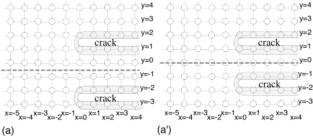
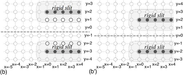
Figure 3: Square lattice with the broken vertical bonds between (with ${N}=2$) (a) ${\mathtt{y}}=\pm{N},{\mathtt{y}}=\pm{N}-1,$ for all ${\mathtt{x}}\geq 0,$ (a’) ${\mathtt{y}}=\pm{N},{\mathtt{y}}=\pm{N}\mp 1$,for all ${\mathtt{x}}\geq 0,$ the constrained sites located (with ${N}=2$) at (b) ${\mathtt{y}}=\pm{N}-{\tfrac{1}{2}}\pm{\tfrac{1}{2}},$ for all ${\mathtt{x}}\geq 0,$ (b’) ${\mathtt{y}}=\pm{N}$, for all ${\mathtt{x}}\geq 0.$

In order to utilize the geometric symmetry in the physical structure, it is natural to consider the even/odd symmetry relative the mid-plane (shown by thick dashed line in Fig. 3). According to (2.1), with odd number of rows in-between the defects, the waveguide width ${N_{w}}$ is $2{N}-1$, on the other hand for the even number of rows in-between, the corresponding waveguide width formed by the two rigid constraints and by the two cracks is ${N_{w}}=2{N}$. The main idea behind the reduction to lattice-half plane can be understood as follows.

Consider the (bulk) incident wave (2). Recall Fig. 4. Two cases arise depending on the even/odd parity of the separation between the two cracks or rigid constraints. For $({\mathtt{x}},{\mathtt{y}})\in{{{\mathbb{Z}}^{2}}}$,

$${\mathtt{u}}_{{\mathtt{x}},{\mathtt{y}}}^{\operatorname{i}B} = {\tfrac{1}{2}}({\mathtt{u}}_{{\mathtt{x}},{\mathtt{y}}}^{\operatorname{i}B}+{\mathtt{u}}_{{\mathtt{x}},-{\mathtt{y}}-1}^{\operatorname{i}B})+{\tfrac{1}{2}}({\mathtt{u}}_{{\mathtt{x}},{\mathtt{y}}}^{\operatorname{i}B}-{\mathtt{u}}_{{\mathtt{x}},-{\mathtt{y}}-1}^{\operatorname{i}B})$$ (3.1a)

$$= {{\mathrm{A}}}e^{i{\upkappa}_{x}{\mathtt{x}}}e^{-i{\tfrac{1}{2}}{\upkappa}_{y}}\cos{\upkappa}_{y}({\mathtt{y}}+{\tfrac{1}{2}})+i{{\mathrm{A}}}e^{i{\upkappa}_{x}{\mathtt{x}}}e^{-i{\tfrac{1}{2}}{\upkappa}_{y}}\sin{\upkappa}_{y}({\mathtt{y}}+{\tfrac{1}{2}}),$$ (3.1b)

and

$${\mathtt{u}}_{{\mathtt{x}},{\mathtt{y}}}^{\operatorname{i}B} = {\tfrac{1}{2}}({\mathtt{u}}_{{\mathtt{x}},{\mathtt{y}}}^{\operatorname{i}B}+{\mathtt{u}}_{{\mathtt{x}},-{\mathtt{y}}}^{\operatorname{i}B})+{\tfrac{1}{2}}({\mathtt{u}}_{{\mathtt{x}},{\mathtt{y}}}^{\operatorname{i}B}-{\mathtt{u}}_{{\mathtt{x}},-{\mathtt{y}}}^{\operatorname{i}B})$$ (3.2a)

$$= {{\mathrm{A}}}e^{i{\upkappa}_{x}{\mathtt{x}}}\cos{\upkappa}_{y}{\mathtt{y}}+i{{\mathrm{A}}}e^{i{\upkappa}_{x}{\mathtt{x}}}\sin{\upkappa}_{y}{\mathtt{y}}.$$ (3.2b)

The first term in (3.1b) (resp. (3.2b)) is even-symmetric relative to ${\mathtt{y}}=-{\tfrac{1}{2}}$ (resp. ${\mathtt{y}}=0$) while the second term is odd-symmetric. Due to the linearity of the scattering problem, using the uniqueness of the solution stated above in Remark 3, it is clear that the scattered wave field also respects the same symmetry and admits an identical decomposition where its even-symmetric (resp. odd-symmetric) component corresponds to even-symmetric (resp. odd-symmetric) component of incident wave.

For the even symmetry of the wave field (incident as well as scattered) in case of even separation, the equivalent reduction to lattice half-plane ${{\mathfrak{S}}}_{\text{H}}$ with free boundary condition is, thus, possible since $\mathtt{u}_{{\mathtt{x}},{\mathtt{y}}}=\mathtt{u}_{{\mathtt{x}},-{\mathtt{y}}-1},{\mathtt{y}}\geq 0$ leads to effectively an absence of bond between the rows located at ${\mathtt{y}}=0$ and ${\mathtt{y}}=-1$. Similarly, for the odd symmetry in case of odd separation, the equivalent reduction to lattice half-plane ${{\mathfrak{S}}}_{\text{H}}$ with fixed boundary condition holds since $\mathtt{u}_{{\mathtt{x}},{\mathtt{y}}}=-\mathtt{u}_{{\mathtt{x}},-{\mathtt{y}}},{\mathtt{y}}\geq 0$ leads to a zero displacement condition for the row located at ${\mathtt{y}}=0$.

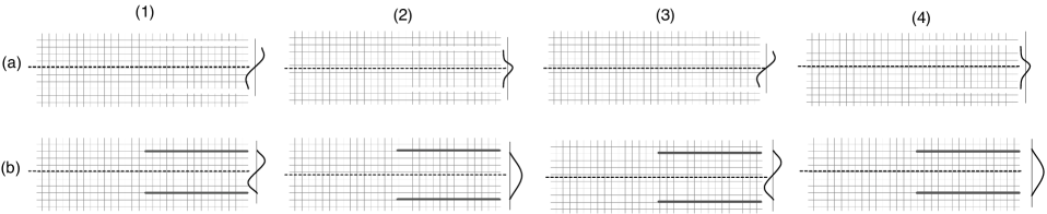
Figure 4: Square lattice with a pair of semi-infinite cracks or rigid constraints and geometric symmetry related to the incident and outgoing wave. The labels (1)–(4) correspond to the conditons Case H1–H4.

In the other two cases the problem becomes equivalent to a lattice half-plane problem with a slightly different boundary condition; the details are omitted. See Fig. 4 for a graphical depiction of the geometric symmetry for the context of a pair of semi-infinite defects.

The diffraction problems on infinite lattice ${{\mathfrak{S}}}$ involving a pair of semi-infinite defects have been solved in this paper by reduction to a problem on lattice half-plane ${{\mathfrak{S}}}_{\text{H}}$ with a single semi-infinite defect forming a waveguide with lattice half-plane boundary at ${\mathtt{y}}=0$. For this purpose, consider the following definition Z^2_H:={(x, y): x, y∈Z, y≥0}. The coordinates associated with ${{\mathfrak{S}}}_{\text{H}}$, including a single semi-infinite defect, are illustrated in Fig. 5 (the same can be contrasted with the choice of coordinates for the infinite lattice as shown in Fig. 3). The condition at half-plane boundary is described by two parameters ${\upbeta}$ and ${\upgamma}$ as

1. ${{\upbeta}}=0,{{\upgamma}}=0$ at ${\mathtt{y}}=1$ for infinite lattice (Fig. 3a’, b’), and at ${\mathtt{y}}=0$ for the lattice half-plane the boundary condition uses ${\mathtt{u}}_{\cdot,{\mathtt{y}}{-1}}=0,$

2. ${{\upbeta}}=0,{{\upgamma}}=-1$ at ${\mathtt{y}}=0$ for infinite lattice (Fig. 3a, b) and at ${\mathtt{y}}=0$ for the lattice half-plane the boundary condition uses ${\mathtt{u}}_{\cdot,{\mathtt{y}}-1}=+{\mathtt{u}}_{\cdot,{\mathtt{y}}},$

3. ${{\upbeta}}=0,{{\upgamma}}=1$ at ${\mathtt{y}}=0$ for infinite lattice (Fig. 3a, b) and at ${\mathtt{y}}=0$ for the lattice half-plane the boundary condition uses ${\mathtt{u}}_{\cdot,{\mathtt{y}}-1}=-{\mathtt{u}}_{\cdot,{\mathtt{y}}},$

4. ${{\upbeta}}=1,{{\upgamma}}=0$ at ${\mathtt{y}}=0$ for infinite lattice (Fig. 3a’, b’) and at ${\mathtt{y}}=0$ for the lattice half-plane the boundary condition uses ${\mathtt{u}}_{\cdot,{\mathtt{y}}-1}={\mathtt{u}}_{\cdot,{\mathtt{y}}+1}$.

In a general case, that includes Case H1–H4, for lattice row at the half-plane boundary (${\mathtt{y}}=0$), u_x+1, y+u_x-1, y+u_x, y+1+(ω^2-4)u_x, y+βu_x, y+1-γu_x, y=0. Naturally, the scattering occurs due to a single semi-infinite defect along with an equation of motion (4) (boundary condition) at the edge of the half-plane ${{\mathfrak{S}}}_{\text{H}}$ in the presence of the incident wave (2). In view of the reduction (Fig. 3–Fig. 5), it is convenient to consider a modified expression for the incident wave (derived from (2) using the reduction based on geometric symmetry) that itself satisfies the boundary condition (4); in particular,

$${\mathtt{u}}_{{\mathtt{x}},{\mathtt{y}}}^{\operatorname{i}}{:=}{{\mathrm{A}}}e^{i{\upkappa}_{x}{\mathtt{x}}+i{\upkappa}_{y}{\mathtt{y}}}+c_{B}{{\mathrm{A}}}e^{i{\upkappa}_{x}{\mathtt{x}}-i{\upkappa}_{y}{\mathtt{y}}},\quad\quad({\mathtt{x}},{\mathtt{y}})\in{{{\mathbb{Z}}^{2}}},{\mathtt{y}}\geq 0,$$ (3.3)

where $c_{B}$ is given by

$$c_{B}={\mathtt{C}}_{B}(e^{-i{\upkappa}_{y}}),\quad{\mathtt{C}}_{B}(\zeta){:=}-\frac{\mathscr{F}_{B}(\zeta)}{\mathscr{F}_{B}(\zeta^{-1})},\quad\mathscr{F}_{B}(\zeta)=\zeta-{{\upbeta}}\zeta^{-1}+{{\upgamma}}.$$ (3.4)

Above expression results after simplification of $-e^{-i{\upkappa}_{y}}-c_{B}e^{i{\upkappa}_{y}}+{{\upbeta}}(e^{i{\upkappa}_{y}}+c_{B}e^{-i{\upkappa}_{y}})-{{\upgamma}}(1+c_{B})=0.$

The general case of the scattering problem on a lattice half-plane ${{\mathfrak{S}}}_{\text{H}}$ with above boundary condition (4) involving ${\upbeta}$ and ${\upgamma}$ can be solved using the complex analysis as developed in [Bls9s] and [Bls10mixed]. Details, using similar notation, are provided below while also following the technique introduced in [Bls0, Bls1].

4 Exact solution based on WH method

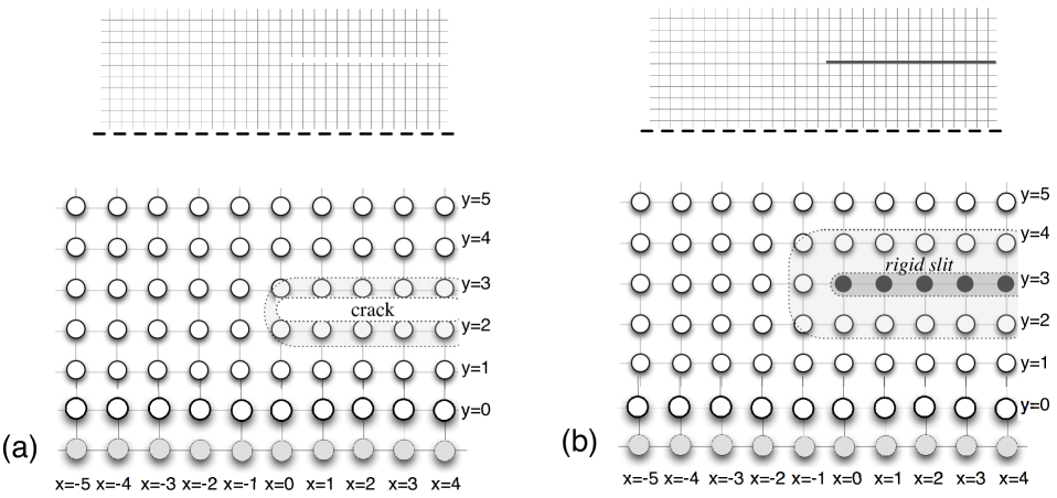
Figure 5: (Top) Reduction based on Fig. 4. (Bottom) Square lattice ${{\mathfrak{S}}}$ with the semi-infinite defect at ${\mathtt{y}}={N}$ ($=3$) and equation of motion (4) at the edge of the half-plane ${{\mathfrak{S}}}_{\text{H}}$ in the presence of the incident wave (2).

Let (recall (4))

$${{\Sigma}}^{\text{H}}_{{k}} {:=} \{{({\mathtt{x}},{\mathtt{y}})\in{{\mathbb{Z}}}^{2}_{\text{H}}:}{\mathtt{x}}\geq 0,{\mathtt{y}}={N},{N}-1\},$$ (4.1a)

$${{\Sigma}}^{\text{H}}_{{c}} {:=} \{{({\mathtt{x}},{\mathtt{y}})\in{{\mathbb{Z}}}^{2}_{\text{H}}:}({\mathtt{x}},{N})\in{{{\mathbb{Z}}^{2}}}:{\mathtt{x}}\geq 0\}.$$ (4.1b)

Above sets correspond to the crack and rigid constraint provided in the schematic illustration of Fig. 5a, b, respectively. The total field ${\mathtt{u}}^{\operatorname{t}}$ at an arbitrary site in ${{\mathfrak{S}}}_{\text{H}}$ is a sum of the incident wave field ${\mathtt{u}}^{\operatorname{i}}$ (3.3) and the scattered field ${\mathtt{u}}^{\operatorname{s}}$. For simplicity, the letter ${\mathtt{u}}$ is used in place of ${\mathtt{u}}^{\operatorname{s}}$. By (2.1) and the definition of ${\upomega}$, the total field ${\mathtt{u}}^{\operatorname{t}}$ satisfies the discrete Helmholtz equation △u^t_x, y+ω^2u^t_x, y=0,  (x, y)∈Z^2_H∖Σ, where u_x, y^t=u_x, y^i+u_x, y, (x, y)∈Z^2, except on the single rigid constraint ${{\Sigma}}{={\Sigma}^{\text{H}}_{{c}}}$ (the equation corresponding to (2.3) holds in the sites near the constraint) or the crack-faces of the single crack ${{\Sigma}}{={\Sigma}^{\text{H}}_{{k}}}$ (where the equation corresponding to (2.2) holds), while at (half-plane boundary) ${\mathtt{y}}=0$ (4) holds.

Let the letter ${{\mathscr{H}}}$ stands for the Heaviside function: ${{\mathscr{H}}}({{\mathtt{x}}})=0,{{\mathtt{x}}}<0$ and ${{\mathscr{H}}}({{\mathtt{x}}})=1,{{\mathtt{x}}\geq 0}$. The discrete Fourier transform [Bls0] of the scattered field $\{{\mathtt{u}}_{{\mathtt{x}},{\mathtt{y}}}\}_{{\mathtt{x}}\in{\mathbb{Z}}}$ at given ${\mathtt{y}}\in{\mathbb{Z}}$ is defined by u_y^F:=u_y; ++u_y; -, u_y; ±=∑_x=-∞^+∞z^-xH(±x-12±12)u_x, y. In this paper, ${{z}}$ denotes the complex variable after the application of Fourier transform. By an application of (discrete) Fourier transform (5) (see also other details in Appendix LABEL:wellposedness), in view of the form of incident wave (3.3) and splitting of the total wave field, the condition (4) at ${\mathtt{y}}=0$ becomes

$$(\operatorname{\mathtt{Q}}+{{\upgamma}}){\mathtt{u}}^{F}_{0}=(1+{{\upbeta}}){\mathtt{u}}^{F}_{1},\quad\quad\text{where }{\operatorname{\mathtt{Q}}}({{z}}){:=}4-{{z}}-{{z}}^{-1}-{\upomega}^{2},{{z}}\in{\mathbb{C}}.$$ (4.2)

(a) Crack

Let ${\mathbb{Z}}_{a}^{b}$ denote the set of integers $\{a,a+1,\dotsc,b\}$. Using the definition of $\lambda$ (LABEL:lambdadef) [Bls0, Bls1, Slepyanbook], the Fourier transform of the (scattered component of the) solution of eq. (4.1) is expressed as u_y^F=u^F_Nλ^y-N,   u_y^F =u^F_0(λ-2N+2λy-λ-yλ-2N+2-1)+u^F_N-1(λ-N+1λ-y-λ-N+1λyλ-2N+2-1). for ${{\mathtt{y}}}\geq{{N}}$ and ${\mathtt{y}}\in{\mathbb{Z}}_{0}^{{N}-1}$, respectively. Note that u_1^F=f_1u^F_0+g_1u^F_N-1, u_N-2^F=f_N-2u