Trans-Neptunian Binaries as Evidence for Planetesimal Formation by the Streaming Instability

A critical step toward the emergence of planets in a protoplanetary disk consists in accretion of planetesimals, bodies 1-1000 km in size, from smaller disk constituents. This process is poorly understood partly because we lack good observational constraints on the complex physical processes that contribute to planetesimal formation [1]. In the outer solar system, the best place to look for clues is the Kuiper belt, where icy planetesimals survived to this day. Here we report evidence that Kuiper belt planetesimals formed by the streaming instability, a process in which aerodynamically concentrated clumps of pebbles gravitationally collapse into $\sim$100-km-class bodies [2]. Gravitational collapse was previously suggested to explain the ubiquity of equal-size binaries in the Kuiper belt [3,4,5]. We analyze new hydrodynamical simulations of the streaming instability to determine the model expectations for the spatial orientation of binary orbits. The predicted broad inclination distribution with $\simeq$80% of prograde binary orbits matches the observations of trans-Neptunian binaries [6]. The formation models which imply predominantly retrograde binary orbits (e.g., [7]) can be ruled out. Given its applicability over a broad range of protoplanetary disk conditions [8], it is expected that the streaming instability seeded planetesimal formation also elsewhere in the solar system, and beyond.

The streaming instability (SI) is a mechanism to seed planetesimal formation by aerodynamically concentrating particles to high densities [2,9-11]. SI simulations show that particle concentration is strong if the (local and height-integrated) solid-to-gas ratio is at least modestly enhanced over solar abundances [10]. Global disk evolution, including photoevaporation, ice lines, pressure traps and other effects (e.g., [12]) can readily produce the required enhancement, suggesting that the SI should commonly operate in protoplanetary disks to hatch planetesimals. Alternately, if the first planetesimals formed with maximum sizes of $\sim$1-10 km (by any mechanism), they can subsequently grow by accreting mass in mutual collisions, a gradual process known as the collisional coagulation (e.g., [13]). Previous attempts to discriminate between different formation processes from the size distribution of planetesimals have been inconclusive [14,15].

We analyze a suite of vertically stratified 3D simulations of the streaming instability (SI) [16,17]. The simulations were performed with the ATHENA code [18], which accounts for the hydrodynamic flow of gas, aerodynamic forces on particles, backreaction of particles on the gas flow, and particle self-gravity. We used the shearing box approximation with at least 512³ gas cells, more than $1.3\times 10^{8}$ particles and appropriate boundary conditions (Methods). Each simulation was parametrized by the dimensionless stopping time of participating particles, $\tau=t_{\rm stop}\Omega$, where $\Omega$ is the Keplerian frequency, and the local particle-to-gas column density ratio, $Z$ (additional parameters are discussed in Methods). We adopted $\tau=0.3$-2, which would correspond to sub-cm-size pebbles in the Minimum Mass Solar Nebula (MMSN; [19]) at 45 au if the gas density was reduced by photoevaporation [12], and $Z=0.02$-0.1. Other choices of these parameters yield similar results [16,17] as long as the system remains in the SI regime [8].

As the time progresses in our simulations (Figure 1), dense azimuthal filaments form, fragment and condense into hundreds of gravitationally-bound clumps. We used an efficient tree-based algorithm (PLAN; Methods) to identify all clumps (Figure 1c). Unfortunately, the resolution in the ATHENA code does not allow us to follow the gravitational collapse of each clump into completion. Instead, we measure the total angular momentum, $J$, and its $z$-component $J_{z}=J\cos\theta$, giving the clump obliquity $\theta$. The total angular momentum can be compared to that of a critically rotating Jacobi ellipsoid: $J_{\rm c}=0.39(GM^{3}r)^{1/2}$ [20], where $G$, $M$ and $r$ are the gravitational constant, mass and effective radius (obtained from $M$ with $\rho=1$ g cm^-3). We find that $J/J_{\rm c}\gg 1$ (this conclusion is insensitive to the choice of density), thus demonstrating that either most of the initial angular momentum must be removed or a typical SI clump cannot collapse into an isolated planetesimal.

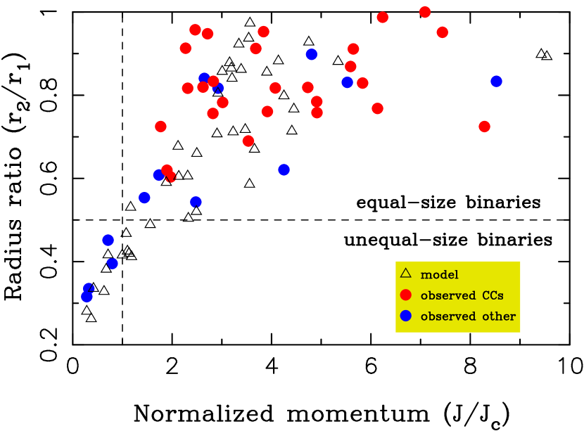
Figure 2: The matching properties of model (triangles) and observed (red and blue dots) binary planetesimals. The model results were taken from new gravitational collapse simulations similar to those reported in ref. [3]. As indicated by our SI simulations, the gravitationally bound clumps have vigorous rotation. Here, we therefore plot cases with the initial rotation $\omega\geq 0.5V_{\rm circ}/R$, where $V_{\rm circ}$ is the circular speed of a particle at the clump radius $R$. The known trans-Neptunian binaries were separated into binaries found among the cold classicals (as defined by the heliocentric orbit inclination $i<5^{\circ}$; red dots) and everything else (blue dots). Note that some of the known unequal-size binaries can be impact generated. The source of the observational data is the Minor Planet Center database.

The vigorous rotation of the SI clumps established here is conducive to the formation of binary planetesimals with properties that closely match observations of the trans-Neptunian binaries. Specifically, in the regime of $J/J_{\rm c}\gg 1$, gravitational collapse is capable of producing a $\sim$100% binary fraction [3] consistent with observations [5]. Binary planetesimals produced by gravitational collapse have nearly equal-size components ($r_{2}/r_{1}>0.5$, where $r_{1}$ and $r_{2}$ are the primary and secondary component radii; Figure 2) and large separations ($a_{\rm b}/(r_{1}+r_{2})>10$, where $a_{\rm b}$ is the binary semimajor axis), just as needed to explain observations [4-6]. Moreover, the matching colors of binary components [21] imply that each binary formed with a uniform compositional mix, as expected for gravitational collapse (but not random capture). Here we elaborate the prediction of the SI model for the spatial orientation of binary orbits.

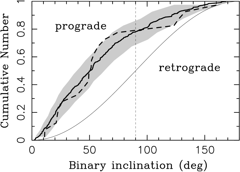
Figure 3: The inclination distribution of binary orbits obtained in the SI model (bold solid line) matches observations of trans-Neptunian binaries (bold dashed line). Here we plot the results of our run A12 at time $t_{\rm sg}=4/\Omega$. The observed inclination distribution shown here includes all CC binaries from ref. [6] with $a_{\rm b}<0.1$ $R_{\rm Hill}$, where $R_{\rm Hill}$ is the Hill radius. Binaries with $a_{\rm b}>0.1$ $R_{\rm Hill}$ are not plotted to limit potential effects of the solar gravity, which may alter wide binary orbits with $i_{\rm b}\sim 90^{\circ}$ (see Supplementary Materials), and gravitational encounters with large bodies [30]. We note that it makes no significant difference whether the wide binaries are included or excluded, because a great majority of known binaries has $a_{\rm b}<0.1$ $R_{\rm Hill}$ (Supplementary Table 1). The shaded area is a 68% envelope of the model results when a sample of 20 model orbits is randomly drawn (i.e., sample size equal to that of real binaries with known inclinations; see Supplementary Figure 5 for a similar comparison with 100 model orbits). The binary orbits are predominantly prograde with $\simeq$80% having $i_{\rm b}<90^{\circ}$. The cumulative distribution of inclinations for randomly oriented binary orbits (thin solid line) is plotted for reference.

The clump obliquities obtained in our SI simulations have a broad distribution (Figure 3) with $\simeq$80% of clumps having $\theta<90^{\circ}$ (prograde rotation relative to the heliocentric orbit) and $\simeq$20% having $\theta>90^{\circ}$ (retrograde rotation). This result is relatively insensitive to various SI parameters (e.g., $\tau$ and $Z$; Methods and Supplementary Figures 1-4) in the regime of strong particle clumping that has been explored. Other concentration mechanisms – e.g., isotropic turbulence or secular gravitational instability – lack concrete predictions for rotation, but are not expected to produce the same distribution of angular momenta by chance. The obliquity distribution shown in Figure 3 is thus a telltale signature of the SI.

To understand how clump obliquities were established, we traced their evolution back in time. Two stages were identified. To get insights into the initial aerodynamic stage, we computed the vorticity of the particle field, $\nabla\times v_{\rm p}$, where $v_{\rm p}$ is the particle velocity. We found that the colatitude distribution of the vorticity vectors of dense particle clumps is broad (Supplementary Figure 4). This is a consequence of the SI that acts to produce the vertical motions needed to tilt the vorticity out of the disk midplane [2,10,17]. The preference for prograde rotation is established during the subsequent stage of gravitational collapse (because prograde clumps become gravitationally bound more often than the retrograde clumps). This preference is consistent, for instance, with gravitational accretion of pebbles onto protoplanets [22]. The clump obliquities change little after the initial collapse phase (Supplementary Figure 2). Thus the imprint of particle concentration by the SI, modified by gravitational collapse, is preserved.

To predict the expected orientation of binary orbits from the SI, we rely on the published results of gravitational collapse simulations [3], where the initial value of $\theta$ was shown to be a good proxy for the binary inclination, $i_{\rm b}$. The clump obliquity distribution can thus be directly compared to the observed distribution of binary inclinations [6]. Here we focus on binaries found in the dynamically cold population of the classical Kuiper belt (hereafter cold classicals, or CCs, defined here as members of the classical main belt with heliocentric orbit inclinations $i<5^{\circ}$; see ref. [23] for a definition of the classical main belt). The CCs are thought to have formed in-situ at $a>40$ au and survived the epoch of planetary migration relatively unharmed [24]. They probably a relatively pristine record of planetesimal formation.

A comparison of the SI-model predicted binary inclinations with observations (Supplementary Table 1) reveals that the two distributions are indistinguishable from each other (Figure 3). Specifically, we implemented the Kolmogorov-Smirnov (K-S) test by comparing the cumulative distribution functions of observed (20) and model (over 400) binaries. The K-S test indicates that the null hypothesis (i.e., the two samples are drawn from the same underlying distribution) cannot be ruled out with more than 13% significance. This comparison clinches an argument in favor of the SI. Crucially, there is a marked $\simeq$4:1 preference for prograde orbits ($i_{\rm b}<90^{\circ}$). For comparison, ref. [7] proposed that the equal-size binaries in the Kuiper belt formed by capture during the coagulation growth of planetesimals. Capture in their model presumably occurred as a result of dynamical friction from a sea of small planetesimals (the L²s mechanism in [7]) or via three-body encounters (the L³ mechanism). These capture models can be ruled out based on the observed inclination distribution of binaries ([6]; Figure 3), because the L²s mechanism predicts retrograde binary orbits with $i_{\rm b}\sim 180^{\circ}$, whereas the L³ mechanism implies a $\sim$3:2 preference for retrograde orbits [25].

The SI is expected to occur over a wide range of protoplanetary disk conditions and pebble sizes [8], which suggests that the planetesimal formation by the SI was widespread. Previous studies explored the SI implications for the initial size distribution (ISD) of planetesimals (e.g., [16,26]), which can be described by a rolling power-law function with an exponential cut-off at large sizes. Attempts to validate the ISD on the size distribution of asteroids and Kuiper belt objects are obscured by secondary processes that modified the distributions after formation (e.g., sustained impact fragmentation, [27]). Here, we point out that the ISD expected from the SI appears to be broadly consistent with the rounded profile of the absolute magnitude distribution of the CCs [28].

The distinctive shape of the New Horizons flyby target (486958) 2014 MU₆₉, which belongs to the CC population, provides additional constraints on the planetesimal formation process. MU₆₉ is a contact binary consisting of two lenticular lobes, roughly $22\times 20\times 7$ km and $14\times 14\times 10$ km in size, connected by a narrow neck [29]. The New Horizons team have been interpreting the shape as resulting from gentle gravitational collapse [29]. The CC binaries apparently span the full range of component separations and sizes from widely separated $\sim$100-km-class binaries to contact/small binaries such as MU₆₉. They are the key to understanding the protoplanetary disk conditions at $>$30 au during planetesimal formation.

Corresponding author
David Nesvorný
Southwest Research Institute
1050 Walnut St., Suite 300
Boulder, Colorado 80302
Phone: (303) 546-0023
Email: davidn@boulder.swri.edu

Acknowledgments
The work of D.N. was funded by the NASA Emerging Worlds program. R.L. acknowledges support from NASA grant NNX16AP53H. A.N.Y. acknowledges support from NASA through grant NNX17AK59G and the NSF through grant 1616929. The funding sources of J.B.S. are NASA grants NNX13AI58G, NNX16AB42G, 80NSSC18K0640, and 80NSSC18K0597. W.M.G contribution was supported in part by NASA Keck PI Data Awards, administrated by the NASA Exoplanet Science Institute and in part by data analysis grants from the Space Telescope Science Institute (STScI), operated by the Association of Universities for Research in Astronomy, Inc., (AURA) under NASA contract NAS 5-26555.

Competing Interest Statement
The authors declare no competing interests.

Author contributions
D.N. suggested a comparison of clump obliquities with binary orbit inclinations and prepared the manuscript for publication. R.L. ran one of the ATHENA simulations and performed data analyses with PLAN. A.N.Y developed scaling relations for planetesimal mass estimates. J.B.S. ran two of the ATHENA simulations. W.M.G. provided the data on trans-Neptunian binaries. All authors contributed to the interpretation of the results and writing of this paper.

Author information
Reprints and permissions information is available at www.nature.com/reprints.
Correspondence and requests for materials should be addressed to davidn@boulder.swri.edu.

Methods

ATHENA code
Our numerical simulations use the Athena code. Athena is a second-order accurate, flux-conservative Godunov code for solving (in this particular application) the coupled equations of hydrodynamics and particle dynamics. To properly integrate the gas dynamics, we have employed the dimensionally unsplit corner transport upwind method [31] and the piecewise parabolic method [32] to spatially reconstruct gas quantities in a third order accurate manner. The calculation of numerical fluxes is done via the HLLC Riemann solver [33]. An in-depth description of the base Athena algorithm, along with tests of this algorithm, can be found in ref. [18].

Particles in the Athena code are treated via the super-particle approach, in which each super-particle is a statistical representation of a larger swarm of particles. The super-particles’ (hereafter just ‘particles’ for brevity) equations of motion are integrated via a semi-implicit drift-kick-drift method (see ref. [34]), and the momentum exchange between the particles and gas is handled via the triangular shaped cloud (TSC) scheme [35,36]. This approach maps the particle momentum from the particle locations to the grid-cell centers (where hydrodynamic quantities are handled) and conversely the gas velocity to the particle locations. A detailed description and tests of the particle integration algorithm can be found in ref. [34].

Shearing box
All of our simulations are carried out in the local, shearing box approximation. This approximation treats a co-rotating portion (or “patch”) of an accretion disk of length scale $L\ll R$, where $R$ is the distance from the central star. In this limit, the relevant equations can be expanded into a Cartesian basis $(x,y,z)$, which is defined relative to disk cylindrical coordinates as $x=(R-R_{0})$, $y=R_{0}\phi$, and $z=z$, where $R_{0}$ is a reference distance. Furthermore, appropriate source terms must be added to the equations to account for the non-inertial reference frame of the domain. See ref. [37] for a detailed description of the shearing box and refs. [34,38] for a description of the shearing box within the context of particle-gas calculations.

The co-rotation frequency of the shearing box equals the Keplerian frequency at $R_{0}$, which we define as $\Omega$. In our particular setup, we include the vertical component of the star’s gravity (i.e., the simulations are vertically stratified). All of our simulations also employ the orbital advection (or FARGO) algorithm [39,40] to analytically integrate quantities along the Keplerian shear flow and integrate the perturbed (relative to Keplerian) quantities using the algorithms described above. This is done for both the gas and the particles and improves the speed and accuracy of the code. To preserve epicyclic energy to machine precision, Crank-Nicholson differencing is used to integrate the non-inertial, shearing box source terms. Finally, we assume an isothermal equation of state for simplicity.

Boundary conditions
The boundary conditions of our domain are shearing-periodic in the radial direction, purely periodic in azimuth, and a modified open/outflow in the vertical direction. The radial shearing periodic boundaries are standard in the shearing box set-up [37]. Briefly, particles/gas that exit one radial boundary enter at the opposite boundary but with a displacement in azimuth and a change in angular momentum and energy applied to account for the difference in the orbital position. The modified outflow conditions in the vertical direction consists of exponentially extrapolating the gas density into the ghost zones, as this significantly reduces numerical artifacts [17,38]. Initially, these boundary conditions allow for excellent maintenance of hydrostatic equilibrium. However, as the system evolves, gas will necessarily be lost via these vertical boundaries (particularly since our domain is quite small and thus the gas density at the vertical boundaries is not significantly different from that at the mid-plane). To ensure mass conservation, we renormalize the gas density in every cell at every time step by a factor that ensures total mass conservation.

Crucial to driving the streaming instability is the radial pressure gradient of the gas. However, a global pressure gradient is inconsistent with the radial shearing-periodic boundaries. To circumvent this issue, an inward radial force is applied to the particles. This force creates an inward drift equivalent to that which would occur as particles lose angular momentum to the sub-Keplerian gas in a real disk. This method is widely employed in shearing box calculations of particle-gas mixtures (e.g., [34]) and is well validated.

Particle self-gravity
In order to study the formation of planetesimals, the mutual gravitational attraction between particles must be included. When activated (see below), the gravitational force is added to the particle equations of motion, and this force is calculated from Poisson’s equation. Numerically, Poisson’s equation is solved as follows. The particle mass density is mapped to the grid cell centers using the TSC approach. This density is then mapped to the nearest time at which the radial boundaries are purely periodic (see ref. [37] for a discussion of this mapping and these “periodic points”), after which a 3D FFT is employed to transform Poisson’s equation into Fourier space.

The gravitational potential is then solved in Fourier space, after which it is transformed back to real space using a second 3D FFT and then mapped back to the original non-periodic frame. As our vertical boundaries are open, a Green’s function approach is used to solve Poisson’s equation in the vertical direction (see details in [38,41]). Finally, the gravitational force is calculated by a second-order, central finite difference of the gravitational potential and then mapped from the grid cell centers back to the locations of the particles via TSC. Boundary conditions must also be applied to the gravitational potential, and these are essentially the same as for the gas quantities: shearing-periodic in $x$, purely periodic in $y$, and open in $z$ with the potential extrapolated into the ghost zones via a third-order scheme. The algorithm has been tested rigorously in ref. [38].

Initial conditions
All of our simulations have the following initial conditions. The gas is in hydrostatic balance with vertical gravity, resulting in an initially Gaussian profile

$$\rho_{g}=\rho_{0}\,{\rm exp}\left(\frac{-z^{2}}{2H^{2}}\right)\ ,$$ (1)

where $\rho_{0}$ is the mid-plane gas density, and $H$ is the vertical scale height of the gas. We set the standard gas parameters equal to unity; $\rho_{0}=H=\Omega=c_{\rm s}=1$ ($c_{\rm s}$ is the sound speed).

The particles are initially distributed with a Gaussian vertical profile, with particle scale height $H_{p}=0.02H$, whereas in $x$ and $y$, the particles are uniformly distributed. Initially, all perturbed velocities (gas and particle velocities with the Keplerian shear subtracted) are set to zero. Finally, we introduce random noise (sampled from a uniform distribution) to the particle locations in all three dimensions to seed the streaming instability.

We first run our numerical simulations without particle self-gravity, allowing the streaming instability to fully develop and produce particle clumping. After the streaming instability has saturated (which is generally defined by when the maximum particle density is stochastically varying but statistically constant in time), we switch on self-gravity. This method is done largely for numerical convenience, as particle self-gravity imposes a performance hit on the integration. In other works [38,42], we have verified that the start time of self-gravity does not largely influence the final properties of planetesimals.

Simulation parameters
In general, streaming-induced planetesimal formation calculations can be characterized via four dimensionless quantities [16,42]: the dimensionless stopping time,

$$\tau=t_{\rm stop}\Omega\ ,$$ (2)

which is the ratio of the dimensional stopping time $t_{\rm stop}$ (i.e., the timescale over which particle momentum relative to the gas motion decreases by $1/e$) to the dynamical time $\Omega^{-1}$ and characterizes the gas-particle interaction (for a single particle species in this case), the particle concentration,

$$Z=\frac{\Sigma_{p}}{\Sigma_{g}}\ ,$$ (3)

which is the ratio of the particle mass surface density $\Sigma_{p}$ to the gas surface density $\Sigma_{g}$ (note that this parameter is related to, but not the same as ’metallicity’), and a radial pressure gradient parameter that accounts for the irradiation from the central star and thus the sub-Keplerian rotating gas in real disks,

$$\Pi=\eta v_{\rm K}/c_{\rm s}\ ,$$ (4)

where $v_{\rm K}$ is the Keplerian velocity and $\eta$ is related to the degree to which gas orbital velocities are sub-Keplerian: $v_{\phi}=v_{\rm K}(1-\eta)$ in the shearing box approximation.

When particle self-gravity is activated, an additional parameter comes into play, which is the relative strength of self-gravity to tidal shear. We quantify this relative strength as

$$\tilde{G}=\frac{4\pi G\rho_{0}}{\Omega^{2}}.$$ (5)

This parameter can be related to the Toomre $Q$ via $\tilde{G}=(4/\sqrt{2\pi})Q^{-1}$. Higher values of $\tilde{G}$ (lower values of $Q$), which occur at larger distances from the central star, equate to weaker tidal shear relative to gravitational binding.

Simulation setup
We have run three simulations in total that span a range of $\tau$, $Z$ and resolution. Run B22 has $\tau=2$, $Z=0.1$, and a domain size $L_{x}\times L_{y}\times L_{z}$ = $(0.2H)^{3}$ with resolution $N_{x}\times N_{y}\times N_{z}=512^{3}$. Run C203 has $\tau=0.3$, $Z=0.02$, and a domain size $L_{x}\times L_{y}\times L_{z}$ = $(0.2H)^{3}$ with resolution $N_{x}\times N_{y}\times N_{z}=512^{3}$. Finally, simulation A12 has $\tau=2$, $Z=0.1$, and a domain size $L_{x}\times L_{y}\times L_{z}$ = $0.1H\times 0.1H\times 0.2H$ with resolution $N_{x}\times N_{y}\times N_{z}=512\times 512\times 1024$. All simulations have $\tilde{G}=0.05$, which equates to a Toomre $Q\simeq 32$, $\Pi=0.05$, and are initiated with $N_{\rm par}=1.34\times 10^{8}$ (run A12) or $1.54\times 10^{8}$ particles (B22 and C203).

The relation between particle size and $\tau$ depends on uncertain properties of the gas disk. If, for reference, we adopt values of the MMSN from ref. [43], a cm-size particle at 45 au would have $\tau=0.3$. Ref. [12] argued that CCs formed when the gas density at 45 au was reduced by photoevaporation. If, for example, the gas density was reduced ten fold, the range of $\tau$ adopted here would correspond to sub-cm-size particles. Alternately, ref. [42] considered a gas disk model with surface density $\Sigma(r)\propto 1/r$, outer radius at 500 au, and total mass $M_{\rm disk}=0.05M_{\odot}$, where $M_{\odot}$ is the solar mass. This disk model would give $\tau=0.3$ for a 2.5 mm particle and $\tau=2$ for a 1.7 cm particle (both at 45 au).

Clump identification
To identify and further characterize the properties of planetesimals produced in our simulations, we use a newly developed clump-finding tool, PLanetesimal ANalyzer (PLAN, [44]). It is designed to work with the 3D particle output of Athena and find gravitationally-bound clumps robustly and efficiently. PLAN, which is written in C++ with OpenMP/MPI, is massively parallelized to analyze billions of particles and many snapshots simultaneously.

Briefly, the workflow of our clump-finding algorithm in PLAN is as follows. The approach is based on the halo finder HOP [45], which allows for fast grouping of physically related particles. PLAN first builds a memory-efficient linear Barnes-Hut tree representing all the particles [46,47]. Each particle is then assigned a density computed from the nearest $N_{\rm den}$ particles ($N_{\rm den}=64$ by default). For particles with densities higher than a threshold, $\delta_{\rm outer}=8\rho_{0}/\tilde{G}$, PLAN chains them up towards their densest neighbors repetitively until a density peak is reached. All the particle chains linked to the same density peak are combined to create a group.

PLAN then merges those groups by examining their boundaries to construct a list of bound clumps. Based on the total kinematic and gravitational energies, deeply intersected groups are merged if bound. However, two particle groups with a saddle point less dense than $\delta_{\rm saddle}=2.5\delta_{\rm outer}$ remain separated [45]. Next, PLAN goes through each group — or raw clump — to unbind any contamination (i.e., passing-by and not bound) particles and gather possibly unidentified member particles within its Hill sphere. After discarding those clumps with Hill radii smaller than one hydrodynamic grid cell ($\Delta x$) or density peaks less than $\delta_{\rm peak}=3\delta_{\rm outer}$, PLAN outputs the final list of clumps with their physical properties derived from particles.

Unlike HOP, PLAN does not further diagnose sub-structures within clumps. Most clumps in our simulations are highly-concentrated, where particles often collapse into regions much smaller than the Hill radius but comparable to or smaller than $\Delta x$, invalidating the search for sub-cell structures. The exact internal architecture of self-bound clumps is beyond the scope of this work. Nevertheless, PLAN does a robust job of identifying clumps as seen in this work (Figure 1) and other recent work [42].

Clump properties
In order to determine the inclination of bound clumps, we use PLAN to calculate their angular momenta in the inertial frame by summing up the contribution from each particle [48,49]. Assuming that the $i$-th particle of a clump is located at $(x_{i},y_{i},z_{i})$ relative to the center-of-mass of the clump, the inertial frame angular momentum $\mbox{\boldmath{$J$}}=(J_{x},J_{y},J_{z})$ can be written as

$$J_{x} =\sum\limits_{i}m_{i}(y_{i}\dot{z_{i}}-z_{i}\dot{y_{i}}-\Omega x_{i}z_{i}),$$ (6)

$$J_{y} =\sum\limits_{i}m_{i}(z_{i}\dot{x_{i}}-x_{i}\dot{z_{i}}-\Omega y_{i}z_{i}),$$ (7)

$$J_{z} =\sum\limits_{i}m_{i}[x_{i}\dot{y_{i}}-y_{i}\dot{x_{i}}-\Omega(x_{i}^{2}+y_{i}^{2})],$$ (8)

where $m_{i}$ is the particle mass. The obliquity of such a clump (i.e., the colatitude of $J$) is then calculated from

$$\theta=\langle\mbox{\boldmath{$J$}},\hat{z}\rangle=\cos^{-1}\left(\frac{\mbox{\boldmath{$J$}}\cdot\hat{z}}{|\mbox{\boldmath{$J$}}|}\right)\ .$$ (9)

Code availability
The ATHENA code is available on GitHub (https://github.com/PrincetonUniversity/Athena-Cversion). The PLAN code is available on Zenodo (see ref. [44]).

Data availability
The data that support the plots within this paper and other findings of this study are available from the corresponding author upon reasonable request.

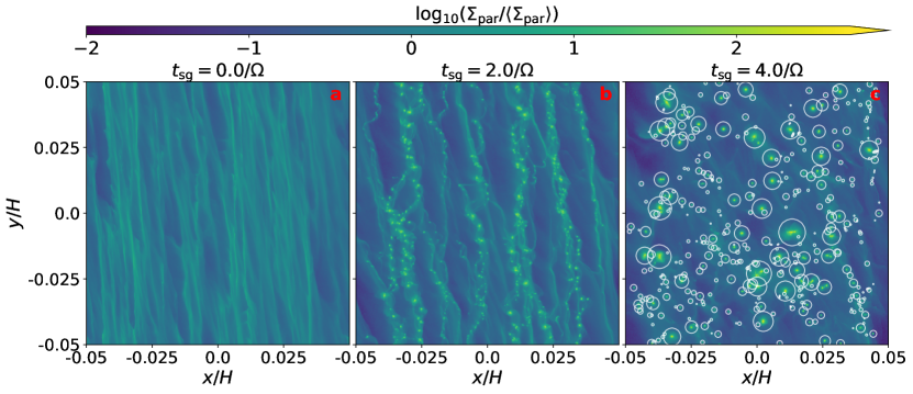
Figure 1: Three snapshots from our 3D simulation of the streaming instability where the nonlinear particle clumping triggers gravitational collapse into planetesimals. The plots show the vertically-integrated density of solids ($\Sigma_{\rm par}$), projected on the disk plane, relative to the initially uniform surface density ($\langle\Sigma_{\rm par}\rangle$). The $x$ and $y$ coordinates show the shearing box dimensions in units of the gas disk scale height, $H$ (the Sun is to the left, the orbital velocity vector points up). Time $t$ increases from left to right as labeled ($t_{\rm sg}=t-t_{0}$; particle self-gravity was switched on at $t_{0}=36/\Omega$). Azimuthal filaments have already formed at $t_{\rm sg}=0$ (panel a). In b and c, the filaments fragment into gravitationally bound clumps. The circles in panel c depict the Hill spheres of clumps that were identified by the PLAN algorithm. The full evolution is shown in the Supplementary Video.

References

- Youdin and Kenyon (2013) [1] Youdin, A. N., Kenyon, S. J. From disks to planets. Planets, Stars and Stellar Systems 3, T. D. Oswalt, L. M. French, and P. Kalas (eds.), Dordrecht, 1-62 (2013).
- Youdin and Goodman (2005) [2] Youdin, A. N., Goodman, J. Streaming instabilities in protoplanetary disks. Astrophys. J. 620, 459-469 (2005).
- Nesvorný et al. (2010) [3] Nesvorný, D., Youdin, A. N., Richardson, D. C. Formation of Kuiper belt binaries by gravitational collapse. Astron. J. 140, 785-793 (2010).
- Noll et al. (2008) [4] Noll, K. S., Grundy, W. M., Chiang, E. I., Margot, J.-L., Kern, S. D. Binaries in the Kuiper belt. The Solar System Beyond Neptune, M. A. Barucci, H. Boehnhardt, D. P. Cruikshank, and A. Morbidelli (eds.), Tucson, 345-363 (2008).
- Fraser et al. (2017) [5] Fraser, W. C. et al. All planetesimals born near the Kuiper belt formed as binaries. Nature Astronomy 1, id. 0088 (2017).
- Grundy et al. (2018) [6] Grundy, W. M. et al. Mutual orbit orientations of transneptunian binaries. Icarus, submitted (2019).
- Goldreich et al. (2002) [7] Goldreich, P., Lithwick, Y., Sari, R. Formation of Kuiper-belt binaries by dynamical friction and three-body encounters. Nature 420, 643-646 (2002).
- Yang et al. (2017) [8] Yang, C.-C., Johansen, A., Carrera, D. Concentrating small particles in protoplanetary disks through the streaming instability. Astron. Astrophys. 606, A80 (2017).
- Johansen et al. (2007) [9] Johansen, A., Oishi, J. S., Mac Low, M.-M., Klahr, H., Henning, T., Youdin, A. Rapid planetesimal formation in turbulent circumstellar disks. Nature 448, 1022-1025 (2007).
- Johansen et al. (2009) [10] Johansen, A., Youdin, A., Mac Low, M.-M. Particle clumping and planetesimal formation depend strongly on metallicity. Astrophys. J. Letters 704, L75-L79 (2009).
- Bai and Stone (2010) [11] Bai, X.-N., Stone, J. M. Dynamics of solids in the midplane of protoplanetary disks: implications for planetesimal formation. Astrophys. J. 722, 1437-1459 (2010).
- Carrera et al. (2017) [12] Carrera, D., Gorti, U., Johansen, A., Davies, M. B. Planetesimal formation by the streaming instability in a photoevaporating disk. Astrophys. J. 839, 16 (2017).
- Kenyon and Luu (1998) [13] Kenyon, S. J., Luu, J. X. Accretion in the early Kuiper belt. I. Coagulation and velocity evolution. Astron. J. 115, 2136-2160 (1998).
- Morbidelli et al. (2009) [14] Morbidelli, A., Bottke, W. F., Nesvorný, D., Levison, H. F. Asteroids were born big. Icarus 204, 558-573 (2009).
- Weidenschilling (2011) [15] Weidenschilling, S. J. Initial sizes of planetesimals and accretion of the asteroids. Icarus 214, 671-684 (2011).
- Simon et al. (2017) [16] Simon, J. B., Armitage, P. J., Youdin, A. N., Li, R. Evidence for universality in the initial planetesimal mass function. Astrophys. J. Letters 847, L12-L17 (2017).
- Li et al. (2018) [17] Li, R., Youdin, A. N., Simon, J. B. On the numerical robustness of the streaming instability: particle concentration and gas dynamics in protoplanetary disks. Astrophys. J. 862, 14-29 (2018).
- Stone et al. (2008) [18] Stone, J. M., Gardiner, T. A., Teuben, P., Hawley, J. F., Simon, J. B. Athena: a new code for astrophysical MHD. Astrophys. J. Supplement Series 178, 137-177 (2008).
- Hayashi (1981) [19] Hayashi, C. Structure of the solar nebula, growth and decay of magnetic fields and effects of magnetic and turbulent viscosities on the nebula. Progress of Theoretical Physics Supplement 70, 35-53 (1981).
- Poincaré (1885) [20] Poincaré, H. Mémoires et observations. Sur l’équilibre d’une masse fluide animée d’un mouvement de rotation. Bulletin Astronomique 2, 109-118 (1885).
- Benecchi et al. (2011) [21] Benecchi, S. D., Noll, K. S., Stephens, D. C., Grundy, W. M., Rawlins, J. Optical and infrared colors of transneptunian objects observed with HST. Icarus 213, 693-709 (2011).
- Johansen and Lacerda (2010) [22] Johansen, A., Lacerda, P. Prograde rotation of protoplanets by accretion of pebbles in a gaseous environment. MNRAS 404, 475-485 (2010).
- Gladman et al. (2008) [23] Gladman, B., Marsden, B. G., Vanlaerhoven, C. Nomenclature in the outer solar system. The Solar System Beyond Neptune, M. A. Barucci, H. Boehnhardt, D. P. Cruikshank, and A. Morbidelli (eds.), Tucson, 43-57 (2008).
- Parker and Kavelaars (2010) [24] Parker, A. H., Kavelaars, J. J. Destruction of binary minor planets during Neptune scattering. Astrophys. J. Letters 722, L204-L208 (2010).
- Schlichting and Sari (2008) [25] Schlichting, H. E., Sari, R. The ratio of retrograde to prograde orbits: a test for Kuiper belt binary formation theories. Astrophys. J. 686, 741-747 (2008).
- Johansen et al. (2015) [26] Johansen, A., Mac Low, M.-M., Lacerda, P., Bizzarro, M. Growth of asteroids, planetary embryos, and Kuiper belt objects by chondrule accretion. Science Advances 1, 1500109 (2015).
- Bottke et al. (2005) [27] Bottke, W. F. et al. The fossilized size distribution of the main asteroid belt. Icarus 175, 111-140 (2005).
- Petit et al. (2016) [28] Petit, J.-M. et al. The absolute magnitude distribution of cold classical Kuiper belt objects. AAS/Division for Planetary Sciences Meeting Abstracts 48, 120.16 (2016).
- Stern et al. (2019) [29] Stern, A. et al. Initial results from the New Horizons exploration of 2014 MU69, a small Kuiper belt object. Science, in press (2019).
- Shannon and Dawson (2018) [30] Shannon, A., Dawson, R. Limits on the number of primordial Scattered disc objects at Pluto mass and higher from the absence of their dynamical signatures on the present-day trans-Neptunian populations. MNRAS 480, 1870-1882 (2018).

References

- Colella (1990) [31] Colella, P. Multidimensional upwind methods for hyperbolic conservation laws, J. of Computational Physics 87, 171-200 (1990).
- Colella and Woodward (1984) [32] Colella, P., Woodward, P. R. The piecewise parabolic method (PPM) for gas-dynamical simulations. J. of Computational Physics 54, 174-201 (1984).
- Toro (1999) [33] Toro, E. F. Riemann Solvers and Numerical Models for Fluid Dynamics, Springer-Verlag: Berlin, Heidelberg (1999).
- Bai and Stone (2010) [34] Bai, X.-N., Stone, J. M. Particle-gas dynamics with Athena: method and convergence. Astrophys. J. Supplement Series 190, 297-310 (2010).
- Hockney and Eastwood (1981) [35] Hockney, R. W., Eastwood, J. W. Computer Simulation Using Particles, New York: McGraw-Hill (1981).
- Youdin and Johansen (2007) [36] Youdin, A., Johansen, A. Protoplanetary disk turbulence driven by the streaming instability: linear evolution and numerical methods. Astrophys. J. 662, 613-626 (2007).
- Hawley et al. (1995) [37] Hawley, J. F., Gammie, C. F., Balbus, S. A. Local three-dimensional magnetohydrodynamic simulations of accretion disks. Astrophys. J. 440, 742-763 (1995).
- Simon et al. (2016) [38] Simon, J. B., Armitage, P. J., Li, R., Youdin, A. N. The mass and size distribution of planetesimals formed by the streaming instability. I. The role of self-gravity. Astrophys. J. 822, 55-72 (2016).
- Masset (2000) [39] Masset, F. FARGO: A fast eulerian transport algorithm for differentially rotating disks. Astron. Astrophys. Supplement Series 141, 165-173 (2000).
- Stone and Gardiner (2010) [40] Stone, J. M., Gardiner, T. A. Implementation of the shearing box approximation in Athena. Astrophys. J. Supplement Series 189, 142-155 (2010).
- Koyama and Ostriker (2009) [41] Koyama, H., Ostriker, E. C. Pressure relations and vertical equilibrium in the turbulent, multiphase interstellar medium. Astrophys. J. 693, 1346-1359 (2009).
- Abod (18) [42] Abod, C. P. et al., The mass and size distribution of planetesimals formed by the streaming instability. II. The effect of the radial gas pressure gradient. ArXiv e-prints arXiv:1810.10018 (2018).
- Chiang and Youdin (2010) [43] Chiang, E., Youdin, A. N. Forming planetesimals in solar and extrasolar nebulae. AREPS 38, 493-522 (2010).
-
Li (2018)
[44]
Li, R., PLAN: PLanetesimal ANalyzer v0.2 (2018),
https://doi.org/10.5281/zenodo.1436807 - Eisenstein and Hut (1998) [45] Eisenstein, D. J., Hut, P. HOP: A new group-finding algorithm for N-body simulations. Astrophys. J. 498, 137-142 (1998).
- Morton (1966) [46] Morton, G. M., A Computer Oriented Geodetic Data Base and a New Technique in File Sequencing, International Business Machines Co. (1966).
- Barnes and Hut (1986) [47] Barnes, J., Hut, P. A hierarchical O(N log N) force-calculation algorithm. Nature 324, 446-449 (1986).
- Lissauer and Kary (1991) [48] Lissauer, J. J., Kary, D. M. The origin of the systematic component of planetary rotation. I - Planet on a circular orbit. Icarus 94, 126-159 (1991).
- Dones and Tremaine (1993) [49] Dones, L., Tremaine, S. On the origin of planetary spins. Icarus 103, 67-92 (1993).