Strong ergodicity breaking in aging of mean field spin glasses

Abstract

Out of equilibrium relaxation processes show aging if they become slower as time passes. Aging processes are ubiquitous and play a fundamental role in the physics of glasses and spin glasses and in other applications (e.g. in algorithms minimizing complex cost/loss functions).

The theory of aging in the out of equilibrium dynamics of mean- field spin glass models has achieved a fundamental role, thanks to the asymptotic analytic solution found by Cugliandolo and Kurchan. However this solution is based on assumptions (e.g. the weak ergodicity breaking hypothesis) which have never been put under a strong test until now.

In the present work we present the results of an extraordinary large set of numerical simulations of the prototypical mean-field spin glass models, namely the Sherrington-Kirkpatrick and the Viana-Bray models. Thanks to a very intensive use of GPUs, we have been able to run the latter model for more than $2^{64}$ spin updates and thus safely extrapolate the numerical data both in the thermodynamical limit and in the large times limit.

The measurements of the two-times correlation functions in isothermal aging after a quench from a random initial configuration to a temperature $T<T_{c}$ provides clear evidence that, at large times, such correlations do not decay to zero as expected by assuming weak ergodicity breaking.

We conclude that strong ergodicity breaking takes place in mean-field spin glasses aging dynamics which, asymptotically, takes place in a confined configurational space. Theoretical models for the aging dynamics need to be revised accordingly.

Aging is a fundamental process in out of equilibrium relaxation dynamics. It refers to the observation that relaxation or correlation timescales grow without bound in time, so the system under study looks slower and slower as time goes by. This phenomenon has been initially discovered experimentally in structural glasses (1, 2) and spin glasses (3, 4), but since then it has been found to be a general feature of glassy systems (5, 6).

The importance of observing and properly describing the aging phenomena is due to their strong connection to the energy landscape where the relaxation dynamics takes place. Understanding the relaxation dynamics in more or less rough energy landscapes is a very interesting and essentially still open problem with important applications. Just to highlight a recent and very active topic: the training of artificial neural networks — that have recently proven to be so effective — is performed by minimizing the loss function, i.e. performing a sort of relaxation dynamics in a very high-dimensional space (7, 8).

The dimension of the space where the dynamics takes place is indeed a crucial aspect. While a dynamics relaxing in a low dimensional space can not be too surprising, when the dynamics happens in a very high-dimensional space, our intuition may easily fail in imaging the proper role of entropic and energetic barriers and thus the description of the out of equilibrium dynamics becomes very challenging.

Actually, any statistical mechanics model in the thermodynamic limit does perform a dynamics in a very high-dimensional space. In few fortunate cases (e.g., ordered models undergoing coarsening dynamics (9, 10)) the out of equilibrium dynamics can be well described with a reduced number of parameters. However, in the more general case of disordered models, our understanding is still limited and based either on numerical simulations or on the analytical solution of restricted classes of models: mainly trap and mean field models.

Trap models (11) provide a very simplified description of aging dynamics in disordered systems by assuming that the dynamics proceeds by “jumps” between randomly chosen states. This strong assumption allows for an analytic solution, but it is not clear to what extent the actual microscopic dynamics in a generic disordered model does satisfy such a hypothesis.

In this work we focus on disordered mean field models, in particular on the well-known Sherrington-Kirkpatrick (SK) model (12, 13) defined by the following Hamiltonian

$$H_{\text{\tiny SK}}=-\sum_{i<j}J_{ij}s_{i}s_{j}\,,$$ (1)

where the $N$ Ising spins $s_{i}$ interact pairwise via quenched random Gaussian couplings $J_{ij}\sim\mathcal{N}(0,1/N)$ having zero mean and variance $1/N$. This model is the prototype for disordered models having a continuous phase transition from a paramagnetic phase to a phase with long range spin glass order (in the SK model it takes place at a temperature $T_{c}=1$).

Thanks to the fact that couplings become very weak in the thermodynamic limit, the off-equilibrium dynamics of mean field models can be written in terms of two times correlation and response functions

$$C(t,t^{\prime})=\frac{1}{N}\sum_{i=1}^{N}\langle s_{i}(t)s_{i}(t^{\prime})\rangle\,,\quad R(t,t^{\prime})=\frac{1}{N}\sum_{i=1}^{N}\frac{\partial\langle s_{i}(t)\rangle}{\partial h_{i}(t^{\prime})}\,.$$

The angular brackets represent the average over the dynamical trajectories and an infinitesimal time-dependent field is added to the Hamiltonian as $-\sum_{i}h_{i}s_{i}$ to compute responses.

In the large $N$ limit $C(t,t^{\prime})$ and $R(t,t^{\prime})$ do satisfy a set of integro-differential equations (14, 15) and the solution to these equations provides the typical decay of correlations in a very large sample of the SK model. Although their exact solution is unknown, Cugliandolo and Kurchan (CK) found an ansatz that, under some hypothesis, solves the equations in the large times limit (16). These equations have been rederived rigorously in some particular cases (17).

The CK asymptotic solution has become very popular and its consequences have been investigated in detail (18, 19). It is also often used as the theoretical basis for the analysis of numerical data (20, 21, 22). Notwithstanding its success, the CK solution has never been put under a severe numerical test, due to the difficulties in simulating very large samples of the SK model. In particular we are not aware of any really stringent numerical test on the assumptions made to derive it.

One of the main hypothesis underlying the CK asymptotic solution is that one-time quantities converge to their equilibrium value. This has been further used as a key assumption to derive the connection between statics and dynamics (23). However, this assumption is far from obvious, given the existence of many mean-field models showing a random first order transition (RFOT) where it is apparent how that assumption may be not satisfied: the prototypical model with a RFOT is the spherical $p$-spin model where the energy relaxes to a value far from the equilibrium one if the temperature is below the dynamical transition temperature (15). At variance to models with a RFOT, in spin glass models undergoing a continuous transition the common belief has been to assume convergence to equilibrium, but even these models have an exponential number of states at low enough temperatures (24), and it is not clear why the out of equilibrium dynamics should converge to equilibrium in this case. We remind the reader that the dynamics we are studying is obtained by taking the large $N$ limit first and thus activated processes between states are suppressed.

We want to put under a stringent test the above hypothesis and we find convenient from the numerical point of view to test the so-called weak ergodicity breaking property, stating that for any finite waiting time $t_{w}$ the correlation eventually decays to zero in the large time limit

$$\lim_{t\to\infty}C(t_{w}+t,t_{w})=0\quad\forall t_{w}\,.$$ (2)

The physical meaning of this hypothesis is clear: in an aging system any configuration reached at a finite time is eventually forgotten completely, because the dynamics, although slower and slower, keeps wandering in a large part of the configurations space. A direct consequence of the weak ergodicity breaking is that an aging system does not keep memory of what it did at any finite time, and the “finite time regime” can be eventually integrated out (under a further hypothesis called weak long term memory: the long-time dynamics wipes out the response to any small initial external perturbation), leading to an asymptotic dynamics that is actually decoupled from the finite times regime. This is a key feature that allows to get to the CK solution.

However, looking retrospectively at the literature of the times when the CK solution was derived, one finds that the numerical and experimental evidence were far from definite. While experiments do not probe a mean-field model, the numerics showed that the correlation $C(t_{w}+t,t_{w})$ decays with time $t$ for each waiting time $t_{w}$ considered, but the range of correlations explored was very limited, with correlations always relatively large: $C(t_{w}+t,t_{w})\gtrsim 0.05$ (25, 26) More recently the Janus collaboration succeeded to probe much larger time scales and much smaller correlations (27), but only studying finite dimensional spin glasses for which the mean field solution is not clear to apply.

In the present work we report the results of an unprecedented numerical effort in the study of the out of equilibrium dynamics in mean field spin glasses to check whether some of the hypothesis at the basis of currently available solutions are valid or not.

We started our study by simulating directly the SK model and found some numerical evidence contrasting with the weak ergodicity breaking assumption (these results are presented in detail in the SI). However we soon realized that such a model would prevent us from reaching sizes and times scales large enough to support any solid statement. Indeed the simulation time for such a model scales quadratically with the system size $N$ and rapidly makes the simulation unfeasible.

We then resorted to a spin glass model defined on a sparse graph (requiring simulation times scaling linearly with the system size), similar to the Viana-Bray (VB) model: (28)

$$H_{\text{\tiny VB}}=-\sum_{(ij)\in E}J_{ij}s_{i}s_{j}\,,$$ (3)

where the edge set $E$ defines the interaction graph and the couplings do not need to be rescaled with the system size (as in realistic models). In order to reduce the effects of the spatial heterogeneity in the $H_{\text{\tiny VB}}$ Hamiltonian, we simulate the model on a Random Regular Graph (RRG) of fixed degree 4 and we use couplings of fixed modulus, i.e. $J_{ij}=\pm 1$, with equal probability. We measure self-averaging quantities, and for the very large sizes that we simulate there is no visible dependence on the specific random graph or couplings realization.

One may question whether the out-of-equilibrium dynamics of the VB model is equivalent to the SK case. The common belief about their equivalence is based on the observation that they are both mean field approximations of the same spin glass model. Notice also that the SK model is equivalent to the large degree limit of the VB model (once couplings or temperatures are properly rescaled). However one may also argue instead that the SK and the VB models have a key difference: only in the former the couplings become very weak in the thermodynamic limit and this may produce visible differences in their out-of-equilibrium dynamics. We do not have strong arguments against this point of view and the only conclusive answer is to study both as we do in the present paper and to compare the results. Nonetheless let us argue that if the out-of-equilibrium dynamics of the SK and VB were really asymptotically different this would have important implications, and the VB model should be preferred to the SK model as a mean field approximation to realistic spin glasses. This is one additional reason that convinced us to make such an important numerical effort in understanding the large times out of equilibrium dynamics of the VB model.

Results and discussion

We have simulated the VB model on a RRG of degree 4 at temperature $T=0.8T_{c}$, where $T_{c}=1/\operatorname{atanh}(1/\sqrt{3})$, starting from a random initial configuration. We have measured the correlation function $C(t_{w}+t,t_{w})$ for $t_{w}=2^{2},2^{4},2^{6},2^{8},2^{10},2^{12}$ and very large times $t$. Statistical errors have been strongly reduced averaging over a huge number of samples (see the Method section and the SI for more details).

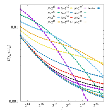
Figure 1: Decay of the two-times correlation function $C(t_{w}+t,t_{w})$ with $t_{w}=4$ in a spin glass defined on a random regular graph of degree 4, initialized in a random configuration and evolved at $T=0.8T_{c}$. We show data for many different system sizes (lines are only a guide to the eye), and the extrapolation to infinite size for every value of $t$ (represented by the series of full symbols at the bottom). It is worth noticing that we are probing a regime of very large times and extremely small correlations, $C(t_{w}+t,t_{w})\ll q_{\text{\tiny EA}}$, never reached before in simulations of mean field models. The upward curvature in the thermodynamic limit is a strong indication against a power law decay to zero correlation, i.e. against the weak ergodicity breaking scenario.

We show in Figure 1 the decay of the correlation function $C(t_{w}+t,t_{w})$ as a function of $t$ for $t_{w}=4$ and a number of different system sizes. The reader should appreciate that we are working in the regime $C(t,t^{\prime})\ll q_{\text{\tiny EA}}\simeq 0.285$ which has never been reached before in any study of the out-of-equilibrium dynamics of mean field spin glass models (the approximate value for $q_{\text{\tiny EA}}$ is obtained via the replica symmetric cavity method). The plot is in a double logarithmic scale, so an upward curvature is a clear indication that correlation is either decaying slower than a power law or not decaying to zero at all.

Let us start discussing equilibration effects. For small enough $N$ we expect the system to thermalize and the correlation function to decay to the equilibrium value $C=0$. The thermalization time $t_{\text{eq}}(N)$ is strongly dependent on the system size $N$ and in Figure 1 it is signalled by the shoulder clearly visible in the data for $2^{12}\leq N\leq 2^{15}$ and partially in the data for $N=2^{16}$. Willing to study the out of equilibrium regime we must impose times to be much smaller than $t_{\text{eq}}$. For $N\geq 2^{18}$ such a thermalization effect is absent for the times we are probing and we can safely consider the data as representative of the out of equilibrium regime.

Figure 1 shows that finite size effects become apparent when measuring very small correlations. Such finite size corrections are otherwise negligibly small at the correlation scale $C\sim 0.1$ which has been the mostly probed one in the past. It is worth noticing that the clear identification of these finite size effects has been possible thanks to the very small uncertainties that we have reached by averaging over a very large number of samples (see the SI for details on simulation parameters) and over a geometrically growing time window: in practice the measurement at time $t$ is the average over the time interval $[t/2^{1/4},t]$.

In order to reach any definite conclusion in the analysis of the out-of-equilibrium dynamics, it is mandatory to take into account these finite size effects accurately in the attempt of extrapolating correlation data to the thermodynamic limit. Indeed, as shown in Figure 1, off-equilibrium correlations measured in a system of smaller size decay asymptotically slower than those measured in a larger system. Then, without taking properly the thermodynamic limit, one can not argue too much about the large time limit of correlation functions. This is the reason why the data we initially got for the SK model, although pointing to the same conclusion we will draw from VB model simulations, were considered not conclusive.

We are interested in the limit of very large times taken after the thermodynamic limit. In this limit we are probing the aging dynamics where activated processes do not play any role. For each fixed time we extrapolate the data shown in Figure 1 to the thermodynamic limit, following the procedure explained in the SI, and we get the curve shown with label “$N\to\infty$” in Figure 1. It is evident that a strong upward curvature remains in the thermodynamical limit, thus suggesting that a power law decay to zero is very unlikely and would require an unnatural very small value of the power law exponent.

Hereafter we concentrate only on the analysis of data already extrapolated to the large $N$ limit. We aim at understanding what is the most likely behavior of the thermodynamic correlation in the limit of large times. We are aware that solely from numerical measurements taken at very large but finite times we cannot make an unassailable statement and one could always claim that on larger times the decay could change. Notwithstanding we believe (and we assume in our analysis) that for the very large times we have reached in our numerical simulations the asymptotic behavior already set in. Thus the results of the analysis should be stable if we change the time window over which the analysis is carried out (always in a way such that $t\gg t_{w}$ and thus $C(t_{w}+t,t_{w})\ll q_{\text{\tiny EA}}$).

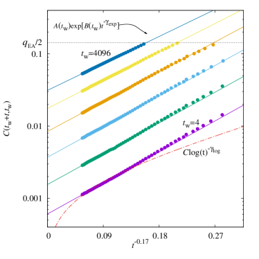
Figure 2: The correlation functions $C(t_{w}+t,t_{w})$ extrapolated in the thermodynamic limit as a function of time $t$, for all the waiting times $t_{w}$ studied. We report only data which are safely in the aging regime $C(t_{w}+t,t_{w})<q_{\text{\tiny EA}}/2$. Straight lines through data points are best fits to functional form in Eq. [4] on the time window $t\in[2^{17},2^{25}]$. The dashed curve is a best fit to a logarithmic decay extrapolating to zero correlation.

In Figure 2 we present the results of the asymptotic analysis that we find most stable and thus most likely, according to the above prescription. The data for the correlations $C(t_{w}+t,t_{w})$ extrapolated in the large $N$ limit are shown as a function of an inverse power of the time for different waiting times, ranging from $t_{w}=4$ to $t_{w}=4096$. We immediately notice that all data follow a nice linear behavior in this scale; the only data departing from the linear behavior are those at very short times, that violate the condition $t_{w}\ll t$. The good agreement with the linear behavior — the lines are fits to data points in $t\in[2^{17},2^{25}]$ — implies that a fit to the form

$$C(t_{w}+t,t_{w})=A(t_{w})\exp\left[B(t_{w})t^{-\gamma_{\text{exp}}}\right]$$ (4)

is very stable upon changing the time window (mind the log scale on the y axis). A joint fit to all $t_{w}$ data with a $t_{w}$-independent exponent gives the value $\gamma_{\text{exp}}\simeq 0.17$, a weakly $t_{w}$-dependent coefficient $B(t_{w})$ and definitely a non-null extrapolations to infinite time $A(t_{w})=\lim_{t\to\infty}C(t_{w}+t,t_{w})$. For a quick reference we may call ‘exponential’ the fit above, although the asymptotic decay is like $A+A\,B\,t^{-\gamma_{\text{exp}}}$.

In order to test the null hypothesis, that is the weak ergodicity breaking scenario where $\lim_{t\to\infty}C(t_{w}+t,t_{w})=0$ for any finite $t_{w}$, we tried to fit the data extrapolated in the large $N$ limit to a function compatible with this limit. Given the upward curvature of the correlation function in a double logarithmic scale (see Figure 1) one may propose a very slow decay according to an inverse power of $\log(t)$. It turns out that a fit to a logarithmic decay $C(t_{w}+t,t_{w})=C(t_{w})\log{(t)^{-\gamma_{\text{log}}}}$, implying a null limiting correlation, yields a value of the sum of squared residuals per degree of freedom one order of magnitude larger than the fit in Eq. [4]. Moreover the values of the fitting exponents are also very strongly dependent on the fitting window (see below and the SI).

The most stricking consequence of the analysis shown in Figure 2 is that, for finite $t_{w}$ values, in the $t\to\infty$ limit the correlation $C(t_{w}+t,t_{w})$ does not decay to zero. This is a very surprising result as it implies — at variance with the widely diffused common belief — that an aging spin glass can asymptotically remember, to some extent, the configurations it reached at finite times. This positive long term correlation confutes the weak ergodicity breaking assumptions and implies a much stronger ergodicity breaking. The present result requires to rethink the asymptotic solutions for the aging dynamics in mean-field spin glass models.

We show now some numerical evidence of why we consider the strong ergodicity breaking as the most likely scenario. In order to test the stability of the fitting procedure with respect to the choice of the time interval, we perform the analysis on intervals $t\in[2^{n-k},2^{n}]$ with fixed $k=6$ and $n$ running on all the time series. A fit to the function $C(t_{w}+t,t_{w})=C(t_{w})\log(t)^{-\gamma_{\text{log}}(t_{w})}$ with $t_{w}$-dependent parameters returns values of $\gamma_{\text{log}}$ that strongly depend on $n$, i.e., on the position of the fitting window (see SI for details). Thus, fit results are very dependent on the time $t$, implying strong corrections to the asymptotic scaling. Again we can not completely exclude this scenario, but it is very unlikely under the hypothesis that corrections to scaling are weak at the very large times we reached at the end of our simulations.

The asymptotic scaling for the correlation decay which has been mostly used until now is an inverse power law of time. Thus we have also fitted our data in the time window $t\in[2^{n-k},2^{n}]$ according to low order polynomials in $t^{-\gamma}$,

$$P_{M}(t_{w}+t,t)=A_{M}(t_{w})+\sum_{m=1}^{M}D_{M}^{(m)}(t_{w})\,t^{-m\gamma_{M}(t_{w})}\;,$$ (5)

with exponents and coefficients depending on both $t_{w}$ and $M$.

Please note that for $D_{M}^{(m)}(t_{w})=A_{M}(t_{w})B_{M}(t_{w})^{m}$ the polynomial in Eq. [5] is nothing but the $M$-th order Taylor expansion of the function in Eq. [4] with $A_{M}(t_{w})=A(t_{w})$ and $B_{M}(t_{w})=B(t_{w})$. It turns out that the identification $D=A\,B^{m}$ is necessary in order to obtain numerically stable results. Moreover assuming such a relation we reduce the number of free parameters and improve correlations among them. At large times, where corrections to the asymptotic scaling should be negligible, the low order polynomials should yield results in agreement with those of the analysis made with the form in Eq. [4]. Any deviation would give a measure of the systematic error introduced by ignoring some corrections terms in the asymptotic behavior.

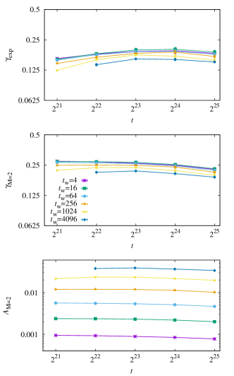
Figure 3: The results of fitting $C(t_{w}+t,t_{w})$ to Eq. [4] (upper panel) and to Eq. [5] with $M=2$ and assuming $D_{M}^{(m)}=A_{M}\,B_{M}^{m}$ (mid and lower panel). In all panels the time on the abscissa $t=2^{n}$ is the upper limit of the fitting range $t\in[2^{n-6},2^{n}]$. We notice that the results of these fitting procedure are very stable, i.e. vary little moving the fitting time window, at variance to fits assuming weak ergodicity breaking.

We report in Fig. 3 the best fitting parameters according to fitting functions in Eq. [4] and in Eq. [5] with $M=2$ and assuming $D_{M}^{(m)}=A_{M}\,B_{M}^{m}$. Results are shown as a function of the upper limit of the time window $[t/2^{6},t]$ where the fit is performed. It is clear that the resulting best fit parameters are very stable, i.e. weakly dependent on the position of the fitting window, and this is a strong indication that we are probing the asymptotic regime with a functional form suffering only tiny finite time corrections. We also notice that the two estimates of the decay exponent $\gamma_{\text{exp}}$ and $\gamma_{M=2}$, shown in the upper and mid panels, become compatible at large times. The asymptotic value for the correlation function $C(\infty,t_{w})$, shown in the lower panel, is very stable too and clearly different from zero.

Analogous fits to any functional form assuming weak ergodicity breaking, that is $C(\infty,t_{w})=0$, return best fitting parameters strongly dependent on the position of the fitting window, and a sum of squared residuals per degree of freedom which is typically one order of magnitude larger than the fits discussed above and illustrated in Fig. 3.

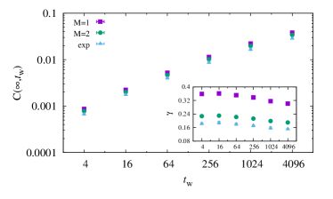
Figure 4: The infinite time limit $C(\infty,t_{w})$ estimated via the most stable fits, that is the one in Eq. [5] with $M=1$ and $M=2$, and the one in Eq. [4]. The fitting range is $t\in[2^{17},2^{25}]$. Inset: the best estimate for the decay exponent.

In conclusion the most likely scenario, which is fully supported by our data, is the one where the limiting value for the correlation function $C(\infty,t_{w})$ is strictly positive for any waiting time $t_{w}$. In Figure 4 we report the estimates of $C(\infty,t_{w})=A_{M}(t_{w})$ obtained from the last fitting window, $t\in[2^{17},2^{25}]$, via the polynomial in Eq. [5] with $M=1$ and $M=2$, together with the values of $A(t_{w})$ obtained via the fit to Eq. [4]. The three estimates are compatible within errors. In the inset of Figure 4 we report the best estimates for the decay exponent obtained from the same fits. The exponent is weakly dependent on $t_{w}$, and systematic errors are more evident, indicating that we are far from a regime in which the decay to the residual correlation can be described by a single power law. Notwithstanding this, different models with different decay exponents agree both qualitatively and quantitatively with a non-null value for the asymptotic correlation.

Computing the value of $C(\infty,t_{w})$ in the large $t_{w}$ limit is out of scope with present data and would require new and longer simulations with larger $t_{w}$ values. However, given that we are working in the aging regime under the condition $C(t_{w}+t,t_{w})<q_{\text{\tiny EA}}$, it is easy to get a conservative upper bound to that limiting correlation, that is $\lim_{t_{w}\to\infty}C(\infty,t_{w})<q_{\text{\tiny EA}}$. Moreover, noticing that the plot in Figure 4 is in double logarithmic scale and that we still do not see any downward curvature, even if correlation values are not far from $q_{\text{\tiny EA}}$, we may conjecture that the upper bound is saturated, that is

$$\lim_{t_{w}\to\infty}C(\infty,t_{w})=q_{\text{\tiny EA}}\,.$$ (6)

The validity of the above conjecture would lead to the unexpected scenario where the out-of-equilibrium relaxation asymptotically gets trapped in an equilibrium state, which is randomly chosen depending on the initial condition and the dynamics at finite times.

The physical picture that emerges from the above strong ergodicity breaking scenario corresponds to a system that, while relaxing in a complex energy landscape, remains confined in regions of the configurations space becoming smaller and smaller during the evolution. Whether this is a single state, a finite set of states or a marginal manifold extending over just a finite fraction of the configurations space is not possible to deduce from our data and further studies will be needed. Nonetheless if this strong ergodicity breaking scenario turns out to be the correct one (as our data strongly suggest) we have to abandon the physical idea of aging as a dynamical process exploring a marginal manifold extending all over the configurations space. The latter scenario can be still perfectly valid for models defined on finite dimensional topologies (e.g. regular lattices) because in that case barriers are not diverging exponentially with the system size and so it is less likely to have a confining potential for the out-of-equilibrium dynamics on finite timescales.

Recently the study of the out-of-equilibrium dynamics in a different mean field spin glass model, namely the spherical mixed $p$-spin, has shown — via analytical solutions — a similar phenomenon (29): depending on the initial condition the asymptotic aging dynamics may take place in a restricted part of the configurations space, and the correlation with configurations at finite times remain strictly positive. This result corroborates those presented in the present work and strongly suggests that, in mean field spin glasses, the most general off-equilibrium relaxation is not the one we had in mind until now (a slow and unbounded wandering in the entire configurational space), but a slow evolution in a confined subspace, determined by the initial condition and the early times dynamics.

In conclusion we have put under a severe test one of the most widely assumed hypothesis in the aging dynamics of mean-field glassy models, namely the weak ergodicity breaking scenario. Our results are clearly in favour of a strong ergodicity breaking scenario, where the two-times correlation function does not decay to zero in the limit of large times. We have been able to achieve such unexpected result, thanks to (i) the use of sparse mean-field spin glass models, (ii) a new careful analysis taking care of both finite size and finite time effects and (iii) an extraordinary numerical effort based on very optimized codes running on latest generation GPUs.

It is fun to notice that the number of spin flips we performed on the largest simulated systems is of the order of $2^{64}$, the same number of wheat grains asked by Sessa, the inventor of chess, to sell his invention. Such an incredibly large number, that determined the destiny of Sessa, allows now to uncover unexpected physics!

Methods

We simulated many samples of the VB model with sizes in the range $2^{10}\leq N\leq 2^{28}$ for times up to $2^{25}$ Monte Carlo sweeps (MCS). We report all details and parameters of the simulations in the SI. Every simulation starts from a random initial configuration and evolves using the Metropolis algorithm at temperature $T=0.8T_{c}=0.8/\operatorname{atanh}{\left(1/\sqrt{3}\right)}\simeq 0.42$ (30). This temperature is a good trade-off because it is not too low (and thus the evolution is not too slow), while being in the low temperature phase and thus having an Edwards-Anderson order parameter $q_{\text{\tiny EA}}$ sensibly different from zero. We remind that the aging dynamics takes place in the large times limit only under the condition $C(t,t^{\prime})<q_{\text{\tiny EA}}$. The thermodynamical properties of typical samples of the VB model can be computed via the cavity method: although for $T<T_{c}$ the exact solution would require to break the replica symmetry in a continuous way, we can get a reasonable approximation to the value of $q_{\text{\tiny EA}}$ via the replica symmetric solution providing $q_{\text{\tiny EA}}(T=0.8T_{c})\simeq 0.285$.

For simulating huge systems for long times it is necessary to resort to parallel processing. To that purpose we implemented the VB model on a random regular bipartite graph (RRBG) making possible to exploit the features of GPU accelerators despite of the very irregular memory access pattern (see SI). We have checked on intermediate sizes that results obtained on RRG and RRBG are statistically equivalent (see results in the SI). The theoretical argument supporting the statistical equivalence of the VB model defined on RRG and RRBG goes as follows: RRG may have loops of any length, while RRBG only have even length loops; since in the VB model with symmetrically distributed couplings (we use $J_{ij}=\pm 1$) every loop can be frustrated with probability $1/2$ independently of its length, we do not expect any difference between the two graph ensembles in the thermodynamic limit, where loops become long. To speed up further the numerical simulations, we resorted to multispin coding techniques where copies evolve in parallel on the same graph, but with different couplings and different initial configurations.

Extrapolations to the thermodynamical limit is an important technical aspect of the present work: we dedicate to it a SI section. The result presented here have been obtained by fitting to a quadratic function $C(N=\infty)+AN^{-\nu}+BN^{-2\nu}$ with $\nu=2/3$. The value of the exponent has been fixed according to well-known results in the literature (31, 32, 33).

The research has been supported by the European Research Council under the EU Horizon 2020 research and innovation programme (grant No. 694925, G. Parisi).

References

References

- (1) Struik L (1976) Physical aging in amorphous glassy polymers. Annals of the New York Academy of Sciences 279(1):78–85.
- (2) Struik L (1977) Physical aging in plastics and other glassy materials. Polymer Engineering & Science 17(3):165–173.
- (3) Mydosh JA (1993) Spin glasses: an experimental introduction. (CRC Press).
- (4) Vincent E, Hammann J, Ocio M, Bouchaud JP, Cugliandolo LF (1997) Slow dynamics and aging in spin glasses in Complex Behaviour of Glassy Systems. (Springer), pp. 184–219.
- (5) Bouchaud JP, Cugliandolo LF, Kurchan J, Mezard M (1998) Out of equilibrium dynamics in spin-glasses and other glassy systems. Spin glasses and random fields pp. 161–223.
- (6) Amir A, Oreg Y, Imry Y (2012) On relaxations and aging of various glasses. Proceedings of the National Academy of Sciences 109(6):1850–1855.
- (7) LeCun Y, Huang FJ (2005) Loss functions for discriminative training of energy-based models. in AIStats. Vol. 6, p. 34.
- (8) Goodfellow I, Bengio Y, Courville A (2016) Deep learning. (MIT press).
- (9) Bray A (2003) Coarsening dynamics of phase-separating systems. Philosophical Transactions of the Royal Society of London. Series A: Mathematical, Physical and Engineering Sciences 361(1805):781–792.
- (10) Cugliandolo LF (2015) Coarsening phenomena. Comptes Rendus Physique 16(3):257–266.
- (11) Bouchaud JP (1992) Weak ergodicity breaking and aging in disordered systems. Journal de Physique I 2(9):1705–1713.
- (12) Sherrington D, Kirkpatrick S (1975) Solvable model of a spin-glass. Physical review letters 35(26):1792.
- (13) Sherrington D, Kirkpatrick S (1978) Infinite-ranged models of spin-glasses. Phys. Rev. B 17(11):4384–4403.
- (14) Crisanti A, Horner H, Sommers HJ (1993) The sphericalp-spin interaction spin-glass model. Zeitschrift für Physik B Condensed Matter 92(2):257–271.
- (15) Cugliandolo LF, Kurchan J (1993) Analytical solution of the off-equilibrium dynamics of a long-range spin-glass model. Physical Review Letters 71(1):173.
- (16) Cugliandolo LF, Kurchan J (1994) On the out-of-equilibrium relaxation of the sherrington-kirkpatrick model. Journal of Physics A: Mathematical and General 27(17):5749.
- (17) Arous GB, Dembo A, Guionnet A (2006) Cugliandolo-kurchan equations for dynamics of spin-glasses. Probability theory and related fields 136(4):619–660.
- (18) Franz S, Mézard M, Parisi G, Peliti L (1998) Measuring equilibrium properties in aging systems. Physical Review Letters 81(9):1758.
- (19) Hérisson D, Ocio M (2002) Fluctuation-dissipation ratio of a spin glass in the aging regime. Physical Review Letters 88(25):257202.
- (20) Franz S, Rieger H (1995) Fluctuation-dissipation ratio in three-dimensional spin glasses. Journal of statistical physics 79(3-4):749–758.
- (21) Marinari E, Parisi G, Ricci-Tersenghi F, Ruiz-Lorenzo JJ, Zuliani F (2000) Replica symmetry breaking in short-range spin glasses: Theoretical foundations and numerical evidences. Journal of Statistical Physics 98(5-6):973–1074.
- (22) Baity-Jesi M, et al. (2017) A statics-dynamics equivalence through the fluctuation–dissipation ratio provides a window into the spin-glass phase from nonequilibrium measurements. Proceedings of the National Academy of Sciences 114(8):1838–1843.
- (23) Franz S, Mezard M, Parisi G, Peliti L (1999) The response of glassy systems to random perturbations: A bridge between equilibrium and off-equilibrium. Journal of statistical physics 97(3-4):459–488.
- (24) Bray A, Moore MA (1980) Metastable states in spin glasses. Journal of Physics C: Solid State Physics 13(19):L469.
- (25) Baldassarri A (1998) Numerical study of the out-of-equilibrium phase space of a mean-field spin glass model. Physical Review E 58(6):7047.
- (26) Marinari E, Parisi G, Rossetti D (1998) Numerical simulations of the dynamical behavior of the sk model. The European Physical Journal B-Condensed Matter and Complex Systems 2(4):495–500.
- (27) Belletti F, et al. (2009) An in-depth view of the microscopic dynamics of ising spin glasses at fixed temperature. Journal of Statistical Physics 135(5-6):1121–1158.
- (28) Viana L, Bray AJ (1985) Phase diagrams for dilute spin glasses. Journal of Physics C: Solid State Physics 18(15):3037.
- (29) Folena G, Franz S, Ricci-Tersenghi F (2019) Memories from the ergodic phase: the awkward dynamics of spherical mixed p-spin models. arXiv preprint arXiv:1903.01421.
- (30) Mézard M, Parisi G (1987) Mean-field theory of randomly frustrated systems with finite connectivity. EPL (Europhysics Letters) 3(10):1067.
- (31) Aspelmeier T, Billoire A, Marinari E, Moore M (2008) Finite-size corrections in the sherrington–kirkpatrick model. Journal of Physics A: Mathematical and Theoretical 41(32):324008.
- (32) Boettcher S (2010) Numerical results for spin glass ground states on bethe lattices: Gaussian bonds. The European Physical Journal B 74(3):363–371.
- (33) Lucibello C, Morone F, Parisi G, Ricci-Tersenghi F, Rizzo T (2014) Finite-size corrections to disordered ising models on random regular graphs. Physical Review E 90(1):012146.