Iterative Qubit Coupled Cluster approach with efficient screening of generators

Abstract

An iterative version of the qubit coupled cluster (QCC) method [I.G. Ryabinkin et al., J. Chem. Theory Comput. 14, 6317 (2019)] is proposed. The new method seeks to find ground electronic energies of molecules on noisy intermediate-scale quantum (NISQ) devices. Each iteration involves a canonical transformation of the Hamiltonian and employs constant-size quantum circuits at the expense of increasing the Hamiltonian size. We numerically studied the convergence of the method on ground-state calculations for LiH, H2O, and N2 molecules and found that the exact ground-state energies can be systematically approached only if the generators of the QCC ansatz are sampled from a specific set of operators. We report an algorithm for constructing this set that scales linearly with the size of a Hamiltonian.

I Introduction

The advent of commercial quantum computers greatly stimulated a desire to use them to solve practically relevant hard computational problems. One such problem is the electronic structure problem Helgaker et al. (2000). Current and near-future quantum computers are noisy intermediate-scale quantum (NISQ) devices Preskill (2018), which are restricted in the number of available qubits, in qubit connectivity, and in the fidelity of single- and multi-qubit entangling gates. Algorithms for such hardware need to minimize the gate count and be able to withstand noise.

Variational quantum eigensolver (VQE) Peruzzo et al. (2014); Wecker et al. (2015) is one such algorithmic framework. It engages both quantum and classical computers in an iterative optimization of the system wave function using the variational principle. The quantum computer constructs a wavefunction guess $\ket{\Psi(\bm{\tau})}={\hat{U}}(\bm{\tau})\ket{0}$ as a sequence of gates representing a parametrized unitary ${\hat{U}}(\bm{\tau})$ acting on some initial qubit wave function $\ket{0}$; $\bm{\tau}$ is a set of numerical parameters. To obtain the expectation value of energy, $E(\bm{\tau})=\braket{\Psi(\bm{\tau})}{\hat{H}}{\Psi(\bm{\tau})}$, the quantum computer performs a series of measurements, which involve $\ket{\Psi(\bm{\tau})}$ and a qubit Hamiltonian $\hat{H}$. $\hat{H}$ is derived from the second-quantized form of the electronic Hamiltonian $\hat{H}_{e}$ of a problem using a fermion-to-qubit transformation. The classical computer accepts the energy estimate $E(\bm{\tau})$ and provides an updated set of parameters, $\bm{\tau}^{\prime}$, to start the next cycle of the algorithm.

The essential component of VQE is a parametrized unitary ${\hat{U}}(\bm{\tau})$ which defines a form (ansatz) of a wave function and determines the accuracy of the method. The VQE does not specify it explicitly; the only practical constraint on ${\hat{U}}(\bm{\tau})$ is its length when expressed in terms of universal qubit gates.

One of the first ansätze explored for VQE was the unitary coupled cluster singles and doubles (UCCSD) form Peruzzo et al. (2014); McClean et al. (2016); O’Malley et al. (2016); Romero et al. (2018); Hempel et al. (2018); Nam et al. (2019). The unitary coupled cluster (UCC) parametrization has several advantages: 1) it is systematically improvable due to its clear fermionic excitation hierarchy, 2) it is size-consistent Crawford and Schaefer III (2007), and 3) it is variational Taube and Bartlett (2006); Evangelista (2011); Harsha et al. (2018). Besides, UCC is highly accurate already at the UCCSD level and rapidly convergent for molecules near equilibrium configurations Olsen (2000); Larsen et al. (2000). However, due to general non-commutativity of involved operators, the UCC form cannot be directly translated into a sequence of quantum gates without an additional Trotter approximation Poulin et al. (2015); Romero et al. (2018). Furthermore, fermionic excitation operators tend to produce redundant terms in the qubit representation Hempel et al. (2018); Nam et al. (2019). This observation together with the NISQ hardware restrictions prompted a search for more efficient UCC forms Lee et al. (2019); Nam et al. (2019).

On the other hand, experimental simulations of small molecules carried out on an existing NISQ device put forward a “hardware-efficient” ansatz Kandala et al. (2017); Barkoutsos et al. (2018), which is a regular, periodic sequence of parametrized single-qubit and fixed-amplitude two-qubit gates. While closely matching the hardware requirements, this ansatz poses a problem of slow convergence with the number of gates. The latter creates an overhead for the classical computer because high-dimensional global minimization with parametrized circuits scales exponentially with the number of dimensions McClean et al. (2018); Lee et al. (2019).

A hardware-oriented approach has stimulated an interest in methods Ryabinkin et al. (2018a); Grimsley et al. (2018) that operate directly in the space of multi-qubit operators:

$$\hat{P}_{k}=\prod_{i}{\hat{\sigma}_{i}^{(k)}},\ \sigma\in\{\hat{1},\hat{x},\hat{y},\hat{z}\}.$$ (1)

One such method, the qubit coupled cluster (QCC), was introduced in our early work Ryabinkin et al. (2018a) and used the following ansatz:

$${\hat{U}}(\bm{\tau})=\prod_{k}\exp(-\mathrm{i}\mkern 1.0mu\tau_{k}\hat{P}_{k}/2).$$ (2)

The total number of $\hat{P}_{k}$s grows exponentially with the number of qubits. Therefore, to select the most relevant $\hat{P}_{k}$s, QCC uses a screening procedure. The screening is based on the energy derivative with respect to the $\hat{P}_{k}$ amplitude, $\tau_{k}$, taken at $\bm{\tau}=0$. Thus, $\hat{P}_{k}$s with the largest energy derivative magnitudes are included in Eq. (2) first. This ranking can be done efficiently on a classical computer. However, the procedure’s simplicity is outweighed by the exponential number of operators that need to be tested, which limits the applicability of the QCC method.

In Ref. 22, the exponential ranking problem of the QCC method was avoided by limiting $\hat{P}_{k}$s to a polynomial number of those that are produced by all single and double fermionic excitations (an “operator pool”). Since this set cannot provide convergence to exact energy (otherwise the UCCSD method would be exact), an iterative scheme was employed: at each iteration, $\hat{P}_{k}$s from the pool are ranked using partial derivatives of energy with the wave function generated at the previous iteration. Calculations of these derivatives are parallelizable, but require a quantum device. Unfortunately, the iterative refinement of the ansatz increases the size of the corresponding quantum circuit, and eventually exhausts the capacity of an NISQ device. Moreover, convergence towards the exact energy is warranted only if all parameters in the ansatz at each iteration are fully re-optimized. The computational cost of this optimization grows exponentially with the number of parameters Lee et al. (2019).

In this work we address two problems. First, how to construct and characterize all operators that have significant energy derivatives without the exponential screening procedure. Second, how to formulate an iterative VQE-type procedure that avoids expansion of a quantum circuit by delegating additional work to the classical computer and performing more measurements. The use of fixed-size quantum circuits will enhance applicability of NISQ devices for solving the electronic structure problem.

The rest of the paper is organized as follows. First, after introducing several prerequisites to the QCC approach, we formulate a new polynomially scaling generator screening procedure. Second, we formulate an iterative QCC scheme and estimate its resource requirements. Third, approaches for reducing the iterative QCC resource requirements are discussed. Fourth, numerical benchmarks for a few molecular systems (LiH, H2O, and N2) are presented.

II Theory

II.1 A few definitions

The QCC method starts at the second-quantized electronic Hamiltonian of a molecule:

$$\hat{H}_{e}=\sum_{ij}^{N_{\text{so}}}h_{ij}{\hat{a}}^{\dagger}_{i}{\hat{a}}_{j}+\frac{1}{2}\sum_{ijkl}^{N_{\text{so}}}g_{ijkl}{\hat{a}}^{\dagger}_{i}{\hat{a}}^{\dagger}_{j}{\hat{a}}_{l}{\hat{a}}_{k},$$ (3)

where ${\hat{a}_{i}}^{\dagger}$ and ${\hat{a}_{i}}$ are fermion creation and annihilation operators, while $h_{ij}$ and $g_{ijkl}$ are molecular one- and two-electrons integrals, written in a spin-orbital basis. The number of spin-orbitals, $N_{\text{so}}$, can be as large as $2N_{\text{AO}}$, twice the number of orbitals in the atomic basis set chosen for a molecule, but in the present work we consider active-space Hamiltonians with $N_{\text{so}}<2N_{\text{AO}}$. To obtain an active-space Hamiltonian one has to prepare a basis of molecular orbitals (MOs), typically by running the Hartree–Fock calculations and then transforming one- and two-electron integrals to that basis. After that, core (always occupied) and frozen virtual (always empty) orbitals must be specified; the contribution of the latter to the Hamiltonian (3) may be simply dropped, while the contribution of the former must be re-calculated explicitly Helgaker et al. (2000). The resulting orbital count is: $N_{\text{so}}=2N_{\text{AO}}-2N_{\text{core}}-2N_{\text{frozen}}$, where factors of 2 account for the doubling of the number of spin-orbitals as compared to the number of spatial orbitals.

For VQE, the electronic Hamiltonian (3) is converted to a qubit form by one of the fermion-to-qubit transformations, Jordan–Wigner (JW) Jordan and Wigner (1928); Aspuru-Guzik et al. (2005) or Bravyi–Kitaev (BK) Bravyi and Kitaev (2002); Seeley et al. (2012); Tranter et al. (2015); Setia and Whitfield (2017); Havlíček et al. (2017)

$$\hat{H}=\sum_{k=1}^{M}C_{k}\hat{P}_{k},$$ (4)

where $C_{k}$ are coefficients, and $\hat{P}_{k}$ are Pauli strings [“words,” see Eq. (1)]. The number of qubits $n$ in $\hat{H}$ is equal to the number of spin-orbitals in the active space, $n=N_{\text{so}}$. The total number of terms in $\hat{H}$, $M$ is $O(n^{4})$, because the fermion-to-qubit transformations map each term of $\hat{H}_{e}$ to the constant number of Pauli words Seeley et al. (2012).

In QCC, an initial state $\ket{0}$ is parametrized as a direct product of $n$ coherent states Radcliffe (1971); Arecchi et al. (1972); Perelomov (2012); Lieb (1973):

$$\ket{\bm{\Omega}} = \prod_{j=1}^{n}\ket{\Omega_{j}},$$ (5)

$$\ket{\Omega_{j}} = \cos\left(\frac{\theta_{j}}{2}\right)\ket{\uparrow}_{j}+\textrm{e}^{\mathrm{i}\mkern 1.0mu\phi_{j}}\sin\left(\frac{\theta_{j}}{2}\right)\ket{\downarrow}_{j},$$ (6)

where $\ket{\uparrow}_{j}$ and $\ket{\downarrow}_{j}$ are eigenstates of $\hat{z}_{j}$, and $\bm{\Omega}=\{\theta_{1},...,\theta_{n}\}\cup\{\phi_{1},...,\phi_{n}\}$ are the corresponding Bloch angles taken as variational parameters. Such a parametrized product state is referred hereinafter as the qubit mean-field (QMF) wave function Ryabinkin et al. (2018b). The total QCC energy is

$$E_{\text{QCC}} =\min_{\bm{\Omega},\bm{\tau}}\braket{\bm{\Omega}}{{\hat{U}}(\bm{\tau})^{\dagger}\hat{H}{\hat{U}}(\bm{\tau})}{\bm{\Omega}}.$$ (7)

To estimate the contribution of each $\hat{P}_{k}$ to $\hat{U}(\bm{\tau})$, one computes a modulus of the QCC energy derivative at $\bm{\tau}=0$:

$$\left|\frac{\mathrm{d}E[\hat{P}_{k}]}{\mathrm{d}\tau_{k}}\Big{|}_{\bm{\tau}=0}\right|$$ (8)

$$= \left|\frac{\mathrm{d}}{\mathrm{d}\tau_{k}}\min_{\bm{\Omega}}\Braket{\bm{\Omega}}{\textrm{e}^{\mathrm{i}\mkern 1.0mu\tau_{k}\hat{P}_{k}/2}\hat{H}\textrm{e}^{-\mathrm{i}\mkern 1.0mu\tau_{k}\hat{P}_{k}/2}}{\bm{\Omega}}\Big{|}_{\tau_{k}=0}\right|$$

$$= \left|\Braket{\text{QMF}}{-\frac{\mathrm{i}\mkern 1.0mu}{2}[\hat{H},\hat{P}_{k}]}{\text{QMF}}\right|\geq 0,$$

where $\ket{\text{QMF}}=\ket{\bm{\Omega}_{\text{min}}}$ is the QMF wave function at the QMF energy minimum.

II.2 Efficient screening procedure

Consider an arbitrary $\hat{P}_{i}$ that satisfies the gradient condition (8). In the absence of external magnetic fields, the electronic Hamiltonian in Eq. (3) is real. This results in real coefficients of $\hat{H}$ and an even number of $\hat{y}$ terms in $\hat{P}_{k}$s. Accounting for this, the energy gradient for $\hat{P}_{i}$ can be rewritten as:

$$\frac{dE[\hat{P}_{i}]}{d\tau}=\sum_{k}C_{k}\,\mathrm{Im}\Braket{\bm{\Omega}_{\text{min}}}{\hat{P}_{k}\hat{P}_{i}}{\bm{\Omega}_{\text{min}}}.$$ (9)

For any $\ket{\bm{\Omega}_{\text{min}}}$, non-vanishing contributions in Eq. (9) can be produced only by $\hat{P}_{k}\hat{P}_{i}$ with purely imaginary matrix elements, requiring $P_{i}$ to have odd powers of $\hat{y}$ terms.

Frequently, the optimized QMF state $\ket{\bm{\Omega}_{\text{min}}}$ is an eigenstate of all $\{\hat{z}_{i}\}_{i=1}^{n}$ operators and, hence, any product of them:

$$\prod_{i}\hat{z}_{i}\ket{\bm{\Omega}_{\text{min}}}=\pm\ket{\bm{\Omega}_{\text{min}}}.$$ (10)

If the lowest-energy QMF solution does not satisfy this condition, one can define a “purified” mean-field state $\ket{\Phi_{0}}$ that satisfies Eq. (10) and has the maximum overlap with the lowest-energy QMF solution. Thus, for further analysis, we will use $\ket{\Phi_{0}}$.

With a property of the independent-qubit reference Eq. (10), the non-vanishing terms in Eq. (9) are the products $\hat{P}_{k}\hat{P}_{i}$ that contain only $\hat{z}$ operations, since

$$\braket{\Phi_{0}}{\hat{f}_{j}}{\Phi_{0}}=0,$$ (11)

where $\hat{f}_{j}\in\{\hat{x}_{j},\hat{y}_{j}\}$ is a generalized flip operator acting on the $j^{\rm th}$ qubit. We denote the flip indices $F(\hat{T})$ of a Pauli term $\hat{P}$ as

$$F(\hat{P})=\{j:\hat{f}_{j}\in\hat{P}\}.$$ (12)

Using Eq. (11) we find that the only non-zero contributions in $[\hat{H},\hat{P}_{i}]$ for a given $\hat{P}_{i}$ are from those $\hat{P}_{k}$s which have the same flip indices as $\hat{P}_{i}$. This leads to partitioning of the original Hamiltonian as

$$\hat{H} =\sum_{k}\hat{S}_{k},$$ (13)

where

$$\hat{S}_{k}=\sum_{j}C_{j}\hat{P}_{j}$$ (14)

group the terms with the same flip indices,

$$F(\hat{P}_{i}) =F(\hat{P}_{j}),\quad\forall(P_{i},\hat{P}_{j})\in\hat{S}_{k}.$$ (15)

Thus, Pauli words possessing the same flip indices introduce an equivalence relation on the set of Hamiltonian terms. As a result, all the generators $\hat{P}_{i}$ with even $\hat{y}$ parity or with $F(\hat{P}_{i})\neq F(\hat{S}_{k}),\forall k$ in Eq. (13) have zero energy gradients. Furthermore, any two generators $\hat{P}_{i}$ and $\hat{P}_{j}$ with the same $\hat{y}$ parity and $F(\hat{P}_{i})=F(\hat{P}_{j})$ will have identical gradients up to a sign, and hence the same gradient magnitudes. Therefore, any generators obtained by replacements of $\hat{1}$ with $\hat{z}$ operators or permutations of $\hat{x}$ and $\hat{y}$ that conserve $\hat{y}$ parity have the same gradient magnitude. This leads to a set of $2^{n-1}$ generators that are characterized by the same absolute energy gradients.

The number of equivalence classes [terms in Eq. (13)] is bound from above by the total number of terms in $\hat{H}$, $M=O(n^{4})$. Thus, the set of all operators that satisfy the gradient condition (8) has the size $O(M2^{n-1})$ with a partitioning into $O(M)$ groups. We will refer to this set as the direct interaction set (DIS).

A representative operator from the DIS can be constructed as follows. First, partition the Hamiltonian as in Eq. (13) by grouping its terms according to their flip indices. Second, for a given $\hat{S}_{k}$ take a product of $\hat{x}$ operators for all but one index from $F(\hat{S}_{k})$, Eq. (12), and multiply it by a single $\hat{y}$ operator with the remaining index. The resulting Pauli word $\hat{P}_{k}$ has the odd (1) number of $\hat{y}$ operators and is characterized by the same flip set as $\hat{S}_{k}$. Third, compute the energy gradient by Eq. (8) by taking $\hat{S}_{k}$ as $\hat{H}$ and $\hat{P}_{k}$ as a candidate; a modulus of the resulting value will characterize the gradient group corresponding to $\hat{S}_{k}$. Finally, repeat these steps for each $\hat{S}_{k}$ to find all representatives and their gradients, thus obtaining the full description of DIS. Since the number of $\hat{S}_{k}$s is bound by the polynomial number of terms in $\hat{H}$ the number of different gradient groups is also polynomial. Due to symmetries encoded in the Hamiltonian coefficients $C_{j}$, some of the representatives can have gradients close to zero.

II.3 The iterative qubit coupled cluster (iQCC)

By rewriting the QCC energy expression (7) as

$$E_{\text{QCC}}=\min_{\bm{\tau}}\left\{\min_{\bm{\Omega}}\braket{\bm{\Omega}}{\hat{H}_{d}(\bm{\tau})}{\bm{\Omega}}\right\},$$ (16)

one demonstrates that the QCC energy is the minimum of the QMF minima for a canonically transformed (“dressed”) Hamiltonian,

$$\hat{H}_{d}(\bm{\tau})=U^{\dagger}(\bm{\tau})\hat{H}{\hat{U}}(\bm{\tau}),$$ (17)

parametrized by the set of amplitudes $\bm{\tau}$. $\hat{H}_{d}(\bm{\tau})$ can be evaluated recursively as

$$\hat{H}_{d}^{(k)}(\tau_{k},\dots,\tau_{1})={} \textrm{e}^{\mathrm{i}\mkern 1.0mu\tau_{k}\hat{P}_{k}/2}\,\hat{H}_{d}^{(k-1)}(\tau_{k-1},\dots,\tau_{1})\,\textrm{e}^{-\mathrm{i}\mkern 1.0mu\tau_{k}\hat{P}_{k}/2}$$

$$={} \hat{H}_{d}^{(k-1)}+\sin\tau_{k}\left(-\frac{\mathrm{i}\mkern 1.0mu}{2}\left[\hat{H}_{d}^{(k-1)},\hat{P}_{k}\right]\right)$$

$$+\frac{1}{2}\left(1-\cos\tau_{k}\right)\left(\hat{P}_{k}\hat{H}_{d}^{(k-1)}\hat{P}_{k}-\hat{H}_{d}^{(k-1)}\right),$$ (18)

where $k=1,\dots,N_{g}$ and $\hat{H}_{d}^{(0)}=\hat{H}$. This procedure produces $3^{N_{g}}$ distinct operator terms and exposes the exponential complexity of the QCC form for a classical computer. However, as shown in Appendix A, if amplitudes $\bm{\tau}$ are fixed, the complexity of the dressing Hamiltonian by Eq. (17) is $\sim M(3/2)^{N_{g}}$.

This observation suggests an iterative reformulation of the QCC procedure. Instead of a single-step optimization of $N_{g}>1$ amplitudes, one can use multiple steps and optimize $N_{g}$ amplitudes sequentially. The number of operators introduced at each step is a constant that can be as low as 1, which means that a quantum circuit of a fixed size can be used at each iteration. However, this iterative formulation does not guarantee the convergence to the exact answer. We did not find rigorous conditions when such convergence was possible and resorted to numerical experiments (see Sec. III).

The iQCC algorithm is summarized below. The number of steps, $N_{\text{steps}}$, and the number of generators, $N_{g}\geq 1$, which will be used at each step, are parameters of the scheme. The initialization step is the QMF energy minimization to determine $E^{(0)}_{\text{QCC}}=E_{\text{QMF}}$ and the initial set of Bloch angles, $\bm{\Omega}^{(0)}$. The iQCC loop is:

1. Run a generator sampling algorithm using the current Hamiltonian $\hat{H}_{d}^{(k-1)}$ and Bloch angles from a previous iteration (to construct the mean-field reference state, $\ket{\bm{\Omega}^{(k-1)}}$) to identify $N_{g}$ generators with the largest absolute gradients in a given pool. If the highest gradient is lower than a threshold, terminate the loop.

2. Minimize the QCC energy, Eq. (7) with respect to $N_{g}$ amplitudes and $2n$ Bloch angles starting from a random guess. If this search with a small (usually  10) number of guesses fails to locate the solution with lower energy than on a previous iteration, perform an additional minimization using $\bm{\tau}=0$ and Bloch angles from the previous iteration as a guess. The last attempt is guaranteed to lower energy because the chosen generators have non-zero energy gradients by construction. The random-search stage is introduced to prevent sticking in local minima and saddle points. You may also terminate the procedure here if the energy difference between the current and previous iterations is below a threshold.

3. Replace the current Hamiltonian by its dressed version calculated by Eq. (II.3) using the $N_{g}$ amplitudes optimized at the current iteration.

4. Compress the resulting Hamiltonian using the techniques from Sec. II.4 (optional).

5. If the number of steps exceeds $N_{\text{steps}}$, exit. Otherwise start a new iteration.

The QCC energy at exit is the final result: the ground-state energy estimate for the Hamiltonian $\hat{H}$.

II.4 Compression of intermediate Hamiltonians

Since the size of the Hamiltonians increases in the course of the iterations, it is natural to seek a method to “compress” them in such a way as to guarantee that their ground-state energies differ less than a desired accuracy $\epsilon$,

$$|E_{0}(\hat{H}_{d}^{(k)})-E_{0}(\hat{H}_{c}^{(k)})|\leq\epsilon.$$ (19)

One can set, for example, $\epsilon=$1\text{\,}\mathrm{m\text{ $E_{\textup{ h }}$ }}$$, which is better than the so-called “chemical accuracy,” $1\text{\,}\mathrm{kcal}\text{\,}{\mathrm{mol}}^{-1}$.

The compression procedure that we propose is based on the Weyl’s spectral perturbation theorem Weyl (1912); Bhatia (1996):

$$\max_{j}|\lambda_{j}^{\downarrow}(\hat{H})-\lambda_{j}^{\downarrow}(\hat{H}_{c})|\leq\|\hat{H}-\hat{H}_{c}\|\leq\|\hat{H}-\hat{H}_{c}\|_{\mathrm{F}},$$ (20)

where $\{\lambda_{j}^{\downarrow}\}$ are eigenvalues of the corresponding operator arranged in decreasing order, $\|\hat{A}\|=\sup_{\|\Psi\|=1}\|\hat{A}\Psi\|$ is the operator norm, which is for a normal (diagonalizable) operator equal to $\max_{j}\{\lambda_{j}\}$, and $\|\hat{A}\|_{\mathrm{F}}=\sqrt{\operatorname{tr}{({\hat{A}}^{\dagger}\hat{A})}}$ is the Frobenius norm of $\hat{A}$ . The Frobenius norm of the qubit Hamiltonian (4) is easy to evaluate:

$$\|\hat{H}\|_{\mathrm{F}}=2^{n/2}\sqrt{\sum_{j}|C_{j}|^{2}},$$ (21)

since $\mathrm{Tr}{({\hat{P}}_{i}^{\dagger}\hat{P}_{j})}=2^{n}\delta_{ij}$, where $\delta_{ij}$ is the Kronecker symbol. Thus, if all $|C_{j}|$ are sorted in descending order, we can define an approximate (compressed) Hamiltonian as

$$\hat{H}_{c}=\sum_{j=1}^{J}C_{j}\hat{P}_{j},$$ (22)

where $J$ satisfes

$$\sqrt{\sum_{j=J+1}|C_{j}|^{2}}\leq\frac{\epsilon}{2^{n/2}}.$$ (23)

At each iteration of the iQCC method one can replace the dressed Hamiltonian $\hat{H}_{d}^{(k)}$ with its compressed version, $\hat{H}_{c}^{(k)}$, to use it as a starting operator for the next iteration. According to inequality (20), this will change the spectrum by no more than $\epsilon$.

The suggested compression procedure is well-suited for use with the iQCC method. As we established in Appendix A, the main reason for growing the dressed Hamiltonians is the commutator term in Eq. (II.3). However, its average value on the QMF wave function is precisely the value of the gradient contribution of the corresponding generator $\hat{P}$, which is systematically reduced by the iQCC procedure. Thus, after the initial rapid growth in size of the intermediate Hamiltonians, one could expect progressively stronger compression when the commutator contributions start systematically falling below the compression threshold $\epsilon$. We verify these expectations numerically in Sec. III.

Table 1: Electronic structure calculations details and parameters of the second-quantized and qubit Hamiltonians for molecules used in the study

Property	Molecule
	LiH	H2O	N2
Molecular configuration	$d(\ce{LiH})=$1.7\text{\,}\mathrm{\SIUnitSymbolAngstrom}$$	$d(\ce{OH})=$1.25$\text{ and }$2.35\text{\,}\mathrm{\SIUnitSymbolAngstrom}$$, $\angle\ce{HOH}=$107.6\text{\,}\mathrm{\SIUnitSymbolDegree}$$	$d(\ce{NN})=$2.118\text{\,}\mathrm{\text{ $a_{0}$ }}$\approx$1.12\text{\,}\mathrm{\SIUnitSymbolAngstrom}$$
Assumed symmetry	$C_{2v}$	$C_{2v}$	$D_{2h}$
Atomic basis set	STO-3G	6-31G	cc-pVDZ
Molecular orbital (MO)set	Hartree–Fock (canonical)
Total number of MOs	6	13	28
Complete active space (CAS)	2e/3orb ($2a_{1}$, $3a_{1}$, $4a_{1}$)	4e/4orb ($1b_{1}$, $3a_{1}$, $4a_{1}$, $2b_{1}$)	10e/8orbs (full valence)
Fermion-to-qubit mapping	parity	Bravyi–Kitaev	parity
Spin-orbital grouping	same spin: first all $\alpha$ then $\beta$
Number of qubits	4	6	14
Length of the qubit $\hat{H}$	100	165	825

III Numerical examples

III.1 Electronic structure calculations and generation of qubit Hamiltonians

Molecular configurations for all species used in this study, as well as the atomic basis sets and active spaces, are listed in Table 1. One- and two-electron integrals for Hamiltonians Eq. (3) in the Hartree–Fock MO basis, were computed by a locally modified version [Feb. 14, 2018 (R1)] of the gamess electronic structure package Schmidt et al. (1993); Gordon and Schmidt (2005). Qubit Hamiltonians were derived from their fermionic counterparts by applying the appropriate fermion-to-qubit transformation (see Table 1). In all cases, the qubit Hamiltonians had stationary qubits Bravyi et al. (2017): namely, qubit operators at positions $N_{\text{so}}$ and $N_{\text{so}}/2$, enter the Hamiltonian as $\hat{z}$ or $\hat{1}$. Thus, $z$-projections of these qubits are constant (stationary), and the corresponding operators can be replaced with their eigenvalues ($\pm 1$) to define qubit-reduced operators. This procedure has been applied to all Hamiltonians, and final qubit counts are listed in Table 1. Eigenvalues of $\hat{z}$ operators for stationary qubits were chosen so as to ensure that the ground states of the full and reduced Hamiltonians are the same. The qubit reduction procedure has also been applied to operators other than a Hamiltonian; see Appendix B.

III.2 LiH and H2O near equilibrium geometry

For small-qubit problems like LiH and H2O, increasing the size of intermediate Hamiltonians poses no difficulties, and no mitigation techniques are necessary. Moreover, rapid convergence of energy in this weak-correlation regime allowed us to gauge the ability of the iQCC method to approach the exact energy. We tested first the most challenging case, $N_{g}=1$, in which only one amplitude is optimized at each iteration. This regime highlights the importance of choosing appropriate generators for the QCC ansatz.

We compare three operator pools: all two-qubit Pauli operators, the operators from spin-adapted single and double fermionic excitation operators transformed to a qubit space (like in Ref. 22), and the DIS. In any case, a single top-gradient [according to Eq. (8)] generator of entanglement was chosen for the QCC ansatz (2) at each iteration.

Convergence of the iQCC procedure with different operator pools is shown in Fig. 1.

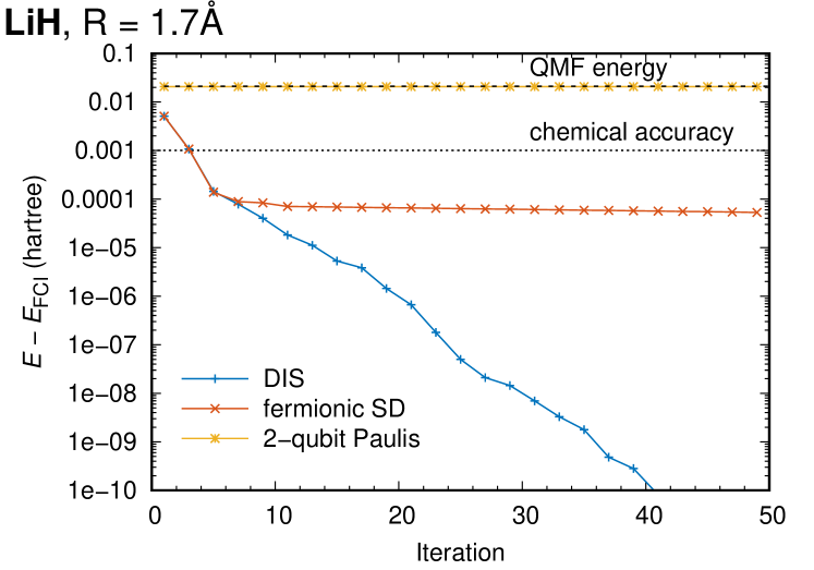
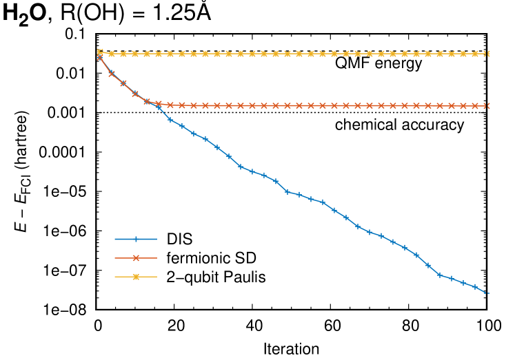
Figure 1: Convergence of a single-generator ($N_{g}=1$) iQCC procedure for various choices of generator pools: “fermionic SD” is a pool of Pauli operators that emerge after a fermion-to-qubit transformation of one- and two-body excitation operators, whereas the “2-qubit Pauli” is the pool of all two-qubit Pauli words.

Energies for non-DIS pools saturate before reaching the exact energy, while DIS provides systematic and almost geometric convergence towards the exact energy. We conjecture that the success of the DIS is due to its additional variational flexibility as it grows together with the growth of intermediate Hamiltonians.

Adding multiple generators

A faster converging setup for the iQCC method is a scheme with the addition of $N_{g}>1$ generators at each step to fully exploit the capabilities of an NISQ device. However, in this case, a problem of degeneracy appears. When generators are subjected to the condition (8), some of them have identical gradient magnitudes and, hence, cannot be ordered. This is a consequence of the structure of the DIS, which is revealed in Sec.  II.2, but to the extent in which the other operator pools overlap with the DIS, it is relevant to them as well. The simplest possible strategy in this situation is a stochastic sampling, in which we draw a single random representative from $N_{g}$ highest-gradient groups. We believe that this procedure reduces the probability of being trapped in local minima.

With multiple generators a faster convergence is observed; see Fig. 2. Only 5 iterations are needed for $N_{g}=6$ to bring the energy closer than $1\text{\times}{10}^{-8}\text{\,}\mathrm{\text{ $E_{\textup{ h }}$ }}$ to exact for the LiH molecule. A similar trend was observed for the H2O molecule (not shown).

Sometimes grouping found less than $N_{g}$ distinct gradient groups. In this case $N_{g}$ is dynamically adjusted to match the number of groups; these numbers are also shown in Fig. 2.

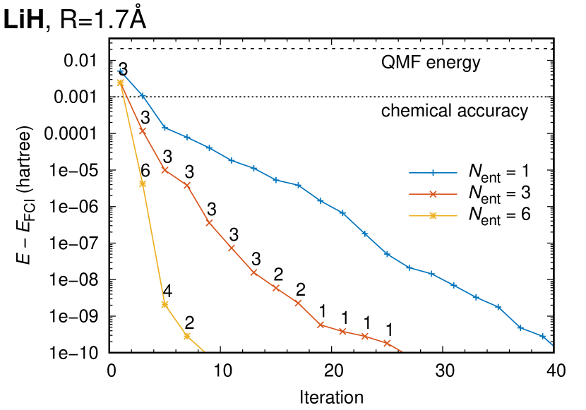
Figure 2: Convergence of the iQCC procedure for different numbers of generators $N_{g}$ from the DIS. The numbers beside each point for $N_{g}>1$ are the numbers of generators chosen by the iterative procedure. They can be less than $N_{g}$ because the number of gradient groups is less than $N_{g}$.

We do not expect this problem to be important for larger-qubit problems, since the number of gradient groups will be much larger than $N_{g}$.

Larger QCC ansatz can also mitigate the issue of premature convergence when the limited operator pools are used. For example, we found (see Fig. 3) that with $N_{g}=6$ the iQCC procedure with sampling from the pool of two-qubit Pauli operators converges to a much lower (albeit not to the exact) energy than the same procedure with $N_{g}=1$ (cf. Fig. 1). Thus, with a more sophisticated QCC form, and a more capable NISQ device the use of limited operator pools may be justified.

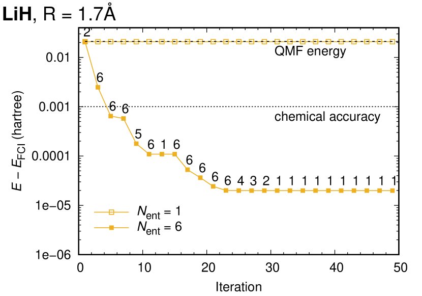
Figure 3: Same as in Fig. 2 but with two-qubit Pauli words as the operator pool.

III.3 Stretched H2O

To assess the iQCC method to treat strong correlation, we consider a stretched H2O molecule with $\ce{R(O-H)}=$2.35\text{\,}\mathrm{\SIUnitSymbolAngstrom}$\approx 2.5\,R_{e}$ . To obtain the singlet QMF solution, we used the penalty method Ryabinkin and Genin (2018), where a spin-penalized Hamiltonian

$$\hat{H}+\frac{\mu}{2}\hat{S}^{2},\ \mu>0$$ (24)

for sufficiently large $\mu$ ($\geq$$0.25\text{\,}\mathrm{\text{ $E_{\textup{ h }}$ }}$) is used. Noticeable deviations from the spin purity in the course of iterations are tolerable because the exact ground state is a singlet, and, as long as the convergence is established, spin deviations vanish.

The convergence of the iQCC procedure with different operator pools is shown in Fig. 4.

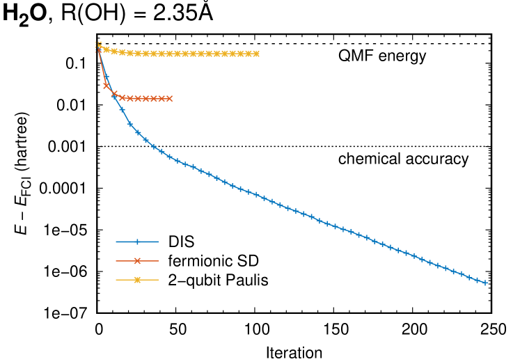
Figure 4: Same as in Fig. 1. For the fermionic and two-qubit Pauli words pools convergence was reached to a given tolerance before the required number of iterations was performed.

Compared to the weak-correlation case (Fig. 1) the convergence is slower. Three times more iterations are necessary to reach similar accuracy with the DIS. Moreover, the initial onset of geometric convergence lasts longer, and the convergence curve is non-linear in the logarithmic scale for the first $\sim 70$ iterations. The other pools exhibit the same behaviour as in the weak-correlation case. They level off before reaching the exact energy. This behaviour is due to a sequential optimization of amplitudes in the ansatz. The amplitudes from earlier iterations cannot be adjusted later. Surprisingly, the number of terms in dressed Hamiltonians at intermediate iterations are comparable between different pools, suggesting that the DIS pool surpasses its competitors by providing more efficient dressing.

III.4 Compression and extrapolation for large-qubit problems

We consider a 14-qubit problem for N2 near the equilibrium geometry (i.e. in the weak-correlation regime) as a prototype for “large-scale” problems. In the tensor-product basis the Hamiltonian matrix has the size $2^{14}\times 2^{14}$, and we expect a rapid growth of the size of intermediate dressed Hamiltonians. This is confirmed by the results in Fig. 5. After 30 iterations, the uncompressed canonically transformed Hamiltonian has $\sim$5\text{\times}{10}^{5}$$ terms.

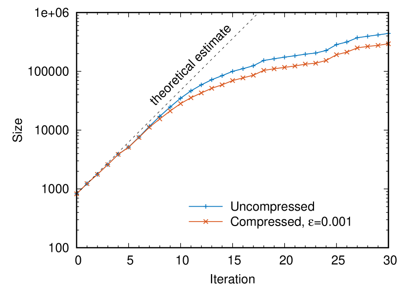
Figure 5: The number of terms of uncompressed and compressed Hamiltonians at each iteration of the iQCC procedure for the N2 molecule with $N_{g}=1$. Theoretical estimate assumes a $M\left(\frac{3}{2}\right)^{\text{Iteration}}$ law derived in Appendix A, where $M=825$ is the size of the initial Hamiltonian (see Table 1).

The onset stage, in which the growth follows the trend predicted in Sec. II.3, $M\left(\frac{3}{2}\right)^{\text{Iteration}}$, continues for the first $~{}10$ iterations. After that the proliferation of terms slows down.

Compression allows one to have $\sim 1.5$ times fewer terms with a negligible impact on energies (Fig. 5). The QCC estimates at iterations differ by less than $3\text{\times}{10}^{-6}\text{\,}\mathrm{\text{ $E_{\textup{ h }}$ }}$ without apparent accumulation of errors. Thus, the spectral compression can be applied with even more aggressive thresholds due to a rather conservative estimate of ground-state disturbance.

Having fewer terms in the Hamiltonian noticeably improves efficiency of the iQCC procedure. However, even after 40 iterations the deviation from the exact energy is more than $1\text{\,}\mathrm{m\text{ $E_{\textup{ h }}$ }}$ (see Fig. 6), so that comparable accuracy in relative energies cannot be guaranteed. Noticing a regular (geometric) convergence pattern of the iQCC energies, we suggest using extrapolation to improve final estimates. This technique gained some popularity, for example, in the density-matrix renormalization group (DMRG) calculations Marti and Reiher (2010).

As evident from Fig. 6, the convergence is close to geometric (linear in the logarithmic scale) after the first $\sim 10$ iterations.

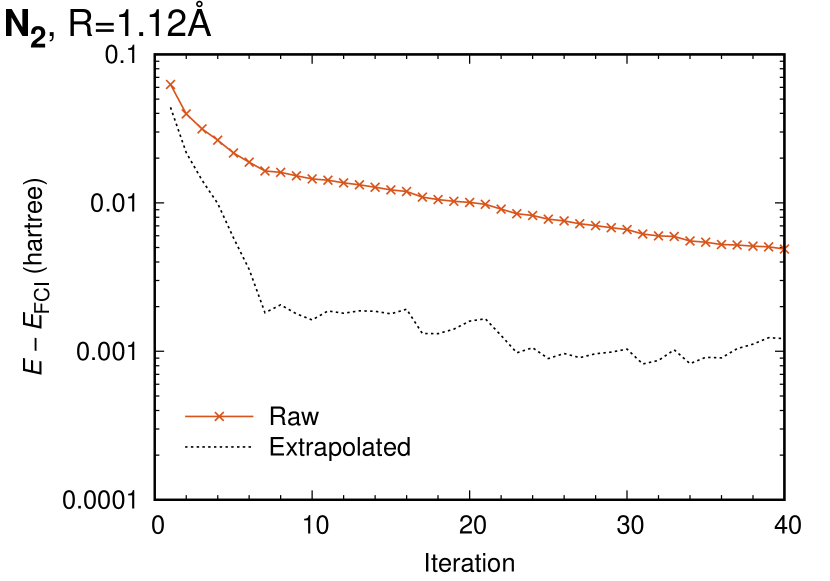
Figure 6: Convergence of raw and extrapolated by Eq. (29) energy estimates for the QCC procedure with $N_{g}=1$.

If one assumes perfect geometric convergence, then

$$\log{\left(E_{\text{QCC}}^{(k)}-E_{\text{exact}}\right)}=ak+b.$$ (25)

Of course, the exact energy $E_{\text{exact}}$ is not known. However, by exponentiating, subtracting, and taking the logarithm again one can obtain

$$\log{\left(E_{\text{QCC}}^{(k-1)}-E_{\text{QCC}}^{(k)}\right)}=a^{\prime}k+b^{\prime},$$ (26)

where

$$a =a^{\prime},$$ (27)

$$b =b^{\prime}-\log{\left(10^{-k^{\prime}}-1\right)}$$ (28)

with an obvious requirement $k^{\prime}<0$. $a^{\prime}$ and $b^{\prime}$ can be determined via the least-square fitting of Eq. (26), and the exact energy estimate at each iteration may be computed as

$$E_{\text{exact}}=E_{\text{QCC}}^{(k)}-10^{(ak+b)}.$$ (29)

We dropped the first 10 values from iQCC iterations and used the remaining ones to fit Eq. (26) and to calculate the extrapolated values by Eq. (29). For the last 10 iterations, the extrapolated value was around $-109.0340\text{\,}\mathrm{\text{ $E_{\textup{ h }}$ }}$, which is $1\text{\,}\mathrm{m\text{ $E_{\textup{ h }}$ }}$ above the exact one $-109.0350\text{\,}\mathrm{\text{ $E_{\textup{ h }}$ }}$, a 5-fold increase in precision as compared to the raw values. Thus, extrapolation may be useful for large-scale iQCC iterations.

IV Conclusions

We have presented and assessed a new technique for the ground-state electronic structure calculations dedicated specifically for use with NISQ devices – the iterative qubit coupled cluster (iQCC)method. It is an iterative modification of our previous technique, the QCC method Ryabinkin et al. (2018a), with a few important amendments.

First, a new selection procedure for generators of the QCC ansatz (2) is proposed. It has computational complexity, which is linear in the number of terms ($M$) of the Hamiltonian, a significant improvement over the previous, exponentially difficult procedure. Apart from that, the new procedure unveiled a non-trivial structure of the set of operators satisfying the QCC selection condition, Eq. (8). This direct interaction set is a union of $O(M)$ groups, each of which contains precisely $2^{n-1}$ operators with identical gradient magnitudes.

Secondly, our numerical experiments indicate that the iQCC procedure converges to the exact energy even with a fixed-size QCC ansatz when the DIS is used as a pool of generators. Compared to competitive approaches, such as the ADAPT-VQE method Grimsley et al. (2018), the QCC method requires neither holding of the whole ansatz on a quantum device nor cumbersome full re-optimization of all its parameters, thus enhancing practical utility of NISQ devices.

It must be admitted that these advantages are not free of cost. The canonical transformation [Eq. (17)] increases the size of the Hamiltonian up to a factor of $3/2$ at each step, which means an increased load on a classical computer and more measurements for a quantum one. Recently, multiple proposals for improving the measurement efficiency have appeared Jena et al. (2019); Verteletskyi et al. (2019); Izmaylov et al. (2019); Huggins et al. (2019); Crawford et al. (2019); Zhao et al. (2019). It would be interesting to apply them to the iQCC intermediate Hamiltonians. To partially compensate an increased load on a classical computer, we introduced two techniques, compression and extrapolation. The first is a rigorous scheme for removing “unimportant” terms from the canonically-transformed Hamiltonians, while the second is inspired by numerical behaviour of the iQCC energy estimates. Both techniques improve the efficiency of large-scale iQCC calculations.

We believe, therefore, that the iQCC method is a viable alternative to other approaches for electronic structure calculations on NISQ devices with the unique feature of employing fixed-size quantum circuits, though its systematic convergence is shown only numerically.

Appendix A Computation scaling of the canonical transformation, Eq. (17)

Consider dressing of the original Hamiltonian $\hat{H}_{d}^{(0)}=\hat{H}$, which has $M=O(n^{4})$ terms, with $\hat{U}(\tau)=\exp(-\mathrm{i}\mkern 1.0mu\tau\hat{P}/2)$, for a fixed value of $\tau$. For $k=1$, Eq. (II.3) contains three distinct operator terms, $\hat{H}$, $[\hat{H},\hat{P}]$, and $\hat{P}\hat{H}\hat{P}$ multiplied by numerical coefficients. First, we notice that the operator $\hat{P}\hat{H}\hat{P}$ has the same operator terms as $\hat{H}$. This is a simple consequence of the anti-commutation relations for Pauli elementary operators: $\hat{\sigma}^{\prime}\hat{\sigma}+\hat{\sigma}\hat{\sigma}^{\prime}=0$ ($\hat{\sigma}\neq\hat{\sigma}^{\prime}$). Multiplying this relation by $\hat{\sigma}$ from the left and using the involutory property, $\hat{\sigma}^{2}=1$, we write:

$$\hat{\sigma}\hat{\sigma}^{\prime}\hat{\sigma}=\begin{cases}-{\hat{\sigma}^{\prime}},&\hat{\sigma}^{\prime}\neq\hat{\sigma}\\ \sigma,&\sigma^{\prime}=\hat{\sigma}.\end{cases}$$ (30)

Thus, every term of $\hat{P}\hat{H}\hat{P}$ has either the same or the opposite sign compared to that in $\hat{H}$. That is, the sum of $\hat{H}$ and $\hat{P}\hat{H}\hat{P}$ with an arbitrary numerical coefficient has no more terms than $\hat{H}$ itself. Therefore, new algebraically independent terms may only come from the commutator term $[\hat{H},\hat{P}]$.

An arbitrary Pauli word commutes with a half and anti-commutes with the remaining half of the $4^{n}$ operators of the $n$-qubit Lie algebra Sarkar and van den Berg (2019). Thus, “on average” the commutator $[\hat{H},\hat{P}]$ will contain only half the terms, $\approx M/2$. In total, we have $\sim\frac{3}{2}M$ terms in $\hat{H}_{d}^{(1)}$ after the dressing with one generator, or $\sim(3/2)^{N_{g}}M$ after a dressing with $N_{g}$ of them.

Appendix B Qubit reduction procedure for general operators

For systems with a small number of qubits, the identification and removal of stationary qubits provide a noticeable reduction of computational complexity. Operators that commute with the Hamiltonian represent exact symmetries. Qubits in such operators can be reduced in the same manner as those in the Hamiltonian; see Sec. III.1. We derived reduced qubit expressions for the total electron number operator, $\hat{N}$, and the total spin operators $\hat{S}_{z}$ and $\hat{S}^{2}$. The corresponding full qubit expressions were derived from the second-quantized counterparts by applying the chosen fermion-to-qubit transformations (see Table 1).

However, not every operator can be reduced, as its symmetry may not be compatible with the symmetry of the Hamiltonian. In particular, the UCC ansatz, whose cluster operators are written in a spin-orbital basis, preserves the electron-number but not the spin symmetry. Some of $\hat{T}$ operators do not commute with $\hat{S}^{2}$. Such operators couple different spin sub-blocks of the Hamiltonian, and their qubit expressions have operators other than $\hat{1}$ or $\hat{z}$ at the position of the stationary qubits. To find reducible combinations, we derived spin-adapted cluster amplitudes following a general scheme given by Eqs. 13.7.2 and 13.7.2 of Ref. 1. In particular, we solved equations

$$[\hat{S}_{\pm},\hat{P}_{k}] =0,$$ (31)

$$[\hat{S}_{z},\hat{P}_{k}] =0,\quad k=1\,\text{(singles)},\ 2\,\text{(doubles)},\ldots$$ (32)

for the qubit expressions of $\hat{P}_{k}$, $\hat{S}_{z}$, and $\hat{S}_{\pm}$ (spin raising/lowering) operators. The solutions are spin-free cluster amplitudes that have stationary qubits at the same positions as the Hamiltonian, and thus can be reduced by the same procedure.

References

- Helgaker et al. (2000) T. Helgaker, P. Jorgensen, and J. Olsen, Molecular Electronic-structure Theory (Wiley, 2000).
- Preskill (2018) J. Preskill, Quantum 2, 79 (2018).
- Peruzzo et al. (2014) A. Peruzzo, J. McClean, P. Shadbolt, M.-H. Yung, X.-Q. Zhou, P. J. Love, A. Aspuru-Guzik, and J. L. O’Brien, Nat. Commun. 5, 4213 (2014).
- Wecker et al. (2015) D. Wecker, M. B. Hastings, and M. Troyer, Phys. Rev. A 92, 042303 (2015).
- McClean et al. (2016) J. R. McClean, J. Romero, R. Babbush, and A. Aspuru-Guzik, New J. Phys. 18, 023023 (2016).
- O’Malley et al. (2016) P. J. J. O’Malley, R. Babbush, I. D. Kivlichan, J. Romero, J. R. McClean, R. Barends, J. Kelly, P. Roushan, A. Tranter, N. Ding, B. Campbell, Y. Chen, Z. Chen, B. Chiaro, A. Dunsworth, A. G. Fowler, E. Jeffrey, E. Lucero, A. Megrant, J. Y. Mutus, M. Neeley, C. Neill, C. Quintana, D. Sank, A. Vainsencher, J. Wenner, T. C. White, P. V. Coveney, P. J. Love, H. Neven, A. Aspuru-Guzik, and J. M. Martinis, Phys. Rev. X 6, 031007 (2016).
- Romero et al. (2018) J. Romero, R. Babbush, J. R. McClean, C. Hempel, P. J. Love, and A. Aspuru-Guzik, Quantum Sci. Technol. 4, 014008 (2018).
- Hempel et al. (2018) C. Hempel, C. Maier, J. Romero, J. McClean, T. Monz, H. Shen, P. Jurcevic, B. P. Lanyon, P. Love, R. Babbush, A. Aspuru-Guzik, R. Blatt, and C. F. Roos, Phys. Rev. X 8, 031022 (2018).
- Nam et al. (2019) Y. Nam, J.-S. Chen, N. C. Pisenti, K. Wright, C. Delaney, D. Maslov, K. R. Brown, S. Allen, J. M. Amini, J. Apisdorf, K. M. Beck, A. Blinov, V. Chaplin, M. Chmielewski, C. Coleman, S. Debnath, A. M. Ducore, K. M. Hudek, M. Keesan, S. M. Kreikemeier, J. Mizrahi, P. Solomon, M. Williams, J. D. Wong-Campos, C. Monroe, and J. Kim, arXiv e-prints (2019), arXiv:1902.10171 .
- Crawford and Schaefer III (2007) T. D. Crawford and H. F. Schaefer III, “An introduction to coupled cluster theory for computational chemists,” in Reviews in Computational Chemistry (John Wiley & Sons, Ltd, 2007) Chap. 2, pp. 33–136, https://onlinelibrary.wiley.com/doi/pdf/10.1002/9780470125915.ch2 .
- Taube and Bartlett (2006) A. G. Taube and R. J. Bartlett, Int. J. Quantum Chem. 106, 3393 (2006).
- Evangelista (2011) F. A. Evangelista, J. Chem. Phys. 134, 224102 (2011).
- Harsha et al. (2018) G. Harsha, T. Shiozaki, and G. E. Scuseria, J. Chem. Phys. 148, 044107 (2018).
- Olsen (2000) J. Olsen, J. Chem. Phys. 113, 7140 (2000).
- Larsen et al. (2000) H. Larsen, J. Olsen, P. Jørgensen, and O. Christiansen, J. Chem. Phys. 113, 6677 (2000).
- Poulin et al. (2015) D. Poulin, M. B. Hastings, D. Wecker, N. Wiebe, A. C. Doberty, and M. Troyer, Quantum Info. Comput. 15, 361 (2015).
- Lee et al. (2019) J. Lee, W. J. Huggins, M. Head-Gordon, and K. B. Whaley, J. Chem. Theory Comput. 15, 311 (2019).
- Kandala et al. (2017) A. Kandala, A. Mezzacapo, K. Temme, M. Takita, M. Brink, J. M. Chow, and J. M. Gambetta, Nature 549, 242 (2017).
- Barkoutsos et al. (2018) P. K. Barkoutsos, J. F. Gonthier, I. Sokolov, N. Moll, G. Salis, A. Fuhrer, M. Ganzhorn, D. J. Egger, M. Troyer, A. Mezzacapo, S. Filipp, and I. Tavernelli, Phys. Rev. A 98, 022322 (2018).
- McClean et al. (2018) J. R. McClean, S. Boixo, V. N. Smelyanskiy, R. Babbush, and H. Neven, Nat. Commun. 9, 4812 (2018).
- Ryabinkin et al. (2018a) I. G. Ryabinkin, T.-C. Yen, S. N. Genin, and A. F. Izmaylov, J. Chem. Theory Comput. 14, 6317 (2018a), arXiv:1809.03827 [quant-ph] .
- Grimsley et al. (2018) H. R. Grimsley, S. E. Economou, E. Barnes, and N. J. Mayhall, arXiv e-prints (2018), arXiv:1812.11173 [quant-ph] .
- Jordan and Wigner (1928) P. Jordan and E. Wigner, Z. Phys. 47, 631 (1928).
- Aspuru-Guzik et al. (2005) A. Aspuru-Guzik, A. D. Dutoi, P. J. Love, and M. Head-Gordon, Science 309, 1704 (2005).
- Bravyi and Kitaev (2002) S. B. Bravyi and A. Y. Kitaev, Ann. Phys. 298, 210 (2002).
- Seeley et al. (2012) J. T. Seeley, M. J. Richard, and P. J. Love, J. Chem. Phys. 137, 224109 (2012).
- Tranter et al. (2015) A. Tranter, S. Sofia, J. Seeley, M. Kaicher, J. McClean, R. Babbush, P. V. Coveney, F. Mintert, F. Wilhelm, and P. J. Love, Int. J. Quantum Chem. 115, 1431 (2015).
- Setia and Whitfield (2017) K. Setia and J. D. Whitfield, ArXiv e-prints (2017), arXiv:1712.00446 [quant-ph] .
- Havlíček et al. (2017) V. Havlíček, M. Troyer, and J. D. Whitfield, Phys. Rev. A 95, 032332 (2017).
- Radcliffe (1971) J. M. Radcliffe, J. Phys. A. 4, 313 (1971).
- Arecchi et al. (1972) F. T. Arecchi, E. Courtens, R. Gilmore, and H. Thomas, Phys. Rev. A 6, 2211 (1972).
- Perelomov (2012) A. Perelomov, Generalized Coherent States and Their Applications, Theoretical and Mathematical Physics (Springer Science & Business Media, 2012).
- Lieb (1973) E. H. Lieb, Commun. Math. Phys. 31, 327 (1973).
- Ryabinkin et al. (2018b) I. G. Ryabinkin, S. N. Genin, and A. F. Izmaylov, J. Chem. Phys. 149, 214105 (2018b), arXiv:1806.00514 [physics.chem-ph] .
- Weyl (1912) H. Weyl, Math. Ann. 71, 441 (1912).
- Bhatia (1996) R. Bhatia, Matrix analysis, Graduate Texts in Mathematics (Springer-Verlag New York, Inc, 1996).
- Note (1) To align our consideration with the Weyl’s theorem, one should use the negate of the real Hamiltonian, .
- Abrams and Sherrill (2005) M. L. Abrams and D. C. Sherrill, Chem. Phys. Lett. 404, 284 (2005).
- Schmidt et al. (1993) M. W. Schmidt, K. K. Baldridge, J. A. Boatz, S. T. Elbert, M. S. Gordon, J. H. Jensen, S. Koseki, N. Matsunaga, K. A. Nguyen, S. J. Su, T. L. Windus, M. Dupuis, and J. Montgomery, J. Comput. Chem. 14, 1347 (1993).
- Gordon and Schmidt (2005) M. S. Gordon and M. W. Schmidt, in Theory and Applications of Computational Chemistry. The first forty years, edited by C. E. Dykstra, G. Frenking, K. S. Kim, and G. E. Scuseria (Elsevier, Amsterdam, 2005) pp. 1167–1189.
- Schuchardt et al. (2007) K. L. Schuchardt, B. T. Didier, T. Elsethagen, L. Sun, V. Gurumoorthi, J. Chase, J. Li, and T. Windus, J. Chem. Inf. Model. 47, 1045 (2007).
- Nielsen (2005) M. A. Nielsen, School of Physical Sciences The University of Queensland (2005).
- Bravyi et al. (2017) S. Bravyi, J. M. Gambetta, A. Mezzacapo, and K. Temme, ArXiv e-prints (2017), arXiv:1701.08213 [quant-ph] .
- Note (2) , is the \ceO-H distance in the water molecule at equilibrium geometry.
- Ryabinkin and Genin (2018) I. G. Ryabinkin and S. N. Genin, arXiv e-prints , arXiv:1812.09812 (2018), arXiv:arXiv:1812.09812 [quant-ph] .
- Marti and Reiher (2010) K. H. Marti and M. Reiher, Mol. Phys. 108, 501 (2010).
- Jena et al. (2019) A. Jena, S. Genin, and M. Mosca, arXiv e-prints , arXiv:1907.07859 (2019), arXiv:1907.07859 [quant-ph] .
- Verteletskyi et al. (2019) V. Verteletskyi, T.-C. Yen, and A. F. Izmaylov, arXiv e-prints , arXiv:1907.03358 (2019), arXiv:1907.03358 [quant-ph] .
- Izmaylov et al. (2019) A. F. Izmaylov, T.-C. Yen, R. A. Lang, and V. Verteletskyi, arXiv e-prints , arXiv:1907.09040 (2019), arXiv:1907.09040 [quant-ph] .
- Huggins et al. (2019) W. J. Huggins, J. McClean, N. Rubin, Z. Jiang, N. Wiebe, K. B. Whaley, and R. Babbush, arXiv e-prints , arXiv:1907.13117 (2019), arXiv:1907.13117 [quant-ph] .
- Crawford et al. (2019) O. Crawford, B. van Straaten, D. Wang, T. Parks, E. Campbell, and S. Brierley, arXiv e-prints , arXiv:1908.06942 (2019), arXiv:1908.06942 [quant-ph] .
- Zhao et al. (2019) A. Zhao, A. Tranter, W. M. Kirby, S. F. Ung, A. Miyake, and P. Love, arXiv preprint arXiv:1908.08067 , 1908.08067 (2019).
- Sarkar and van den Berg (2019) R. Sarkar and E. van den Berg, arXiv e-prints , arXiv:1909.08123 (2019), arXiv:1909.08123 [quant-ph] .