Modeling Embedding Dimension Correlations via Convolutional Neural Collaborative Filtering

Abstract.

As the core of recommender system, collaborative filtering (CF) models the affinity between a user and an item from historical user-item interactions, such as clicks, purchases, and so on. Benefited from the strong representation power, neural networks have recently revolutionized the recommendation research, setting up a new standard for CF. However, existing neural recommender models do not explicitly consider the correlations among embedding dimensions, making them less effective in modeling the interaction function between users and items. In this work, we emphasize on modeling the correlations among embedding dimensions in neural networks to pursue higher effectiveness for CF. We propose a novel and general neural collaborative filtering framework, namely ConvNCF, which is featured with two designs: 1) applying outer product on user embedding and item embedding to explicitly model the pairwise correlations between embedding dimensions, and 2) employing convolutional neural network above the outer product to learn the high-order correlations among embedding dimensions. To justify our proposal, we present three instantiations of ConvNCF by using different inputs to represent a user and conduct experiments on two real-world datasets. Extensive results verify the utility of modeling embedding dimension correlations with ConvNCF, which outperforms several competitive CF methods.

1. Introduction

Recommender system plays a vital role in the era of information explosion. It not only alleviates the information overload issue and facilities the information seeking for users, but also serves as an effective solution to increase the traffic and revenue for service providers. Given its extensive use in Web applications like E-commerce (Yu et al., 2018), social media (Wang et al., 2017), news portal (Wang et al., 2018), and music sites (Cao et al., 2017b), its importance cannot be overstated as a highly valuable learning system. For example, it is reported that about $30\%$ traffic in Amazon are brought by recommendations (Sharma et al., 2015), and the Netflix recommender system has contributed over $1 billion revenue per year (Gomez-Uribe and Hunt, 2016).

Modern recommender systems typically rely on collaborative filtering (and/or its content/context -aware variants) to predict a user’s preference on unknown items (Bayer et al., 2017; He et al., 2019; Deng et al., 2017; Zhao et al., 2018). The learning objective can be abstracted as estimating the affinity score between a user and an item, such that the recommendation list for a user can be obtained by ranking the candidate items according to the affinity scores. Generally speaking, the key to build a CF model lies in twofold: 1) how to represent a user and an item, and 2) how to build the predictive function based on user and item representations. As a pioneering CF model, matrix factorization (MF) (Koren, 2008) embeds a user and an item into vector representations, and formulates the predictive function as the inner product between user embedding vector item embedding vector. Soon after MF was introduced to recommender system, it becomes prevalent in recommendation research with many variants developed. Some representative variants include FISM (factored item similarity model) (Kabbur et al., 2013) and SVD++ (Koren, 2008) which enrich the user embedding with the embeddings of the user’s interacted items, and FM (factorization machine) (Rendle, 2010) and SVDfeature (Chen et al., 2012; Yuan et al., 2018) which extend the predictive function with the inner product between the embeddings of content (and/or context) features.

Without exaggeration, we would say that factorization methods are the most popular approach and play a dominant role in recommendation research in the past decade. In essence, MF leads to the de facto standard for modeling the CF effect — measuring the user-item affinity with inner product in the embedding space. While inner product is effective in capturing the low-rank structure in sparse user-item interaction data (Beutel et al., 2018), its simplicity (i.e., no learnable parameters are involved) and linearity (i.e., no any nonlinear transformations) limit the expressive power of the predictive function. For example, He et al. (He et al., 2017) demonstrated that it may lead to unexpected ranking loss when the embedding size is not sufficiently large, and Hsieh et al. (Hsieh et al., 2017) illustrated the cases that inner product may fail due to its violation of the triangle inequality.

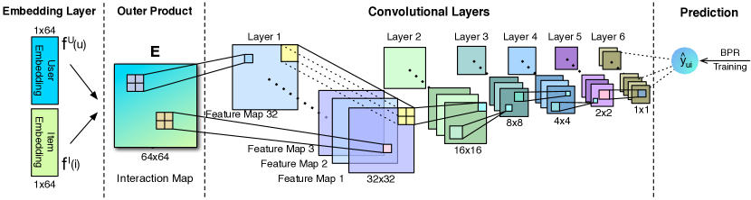
Figure 1. An illustration of our proposed Convolutional Neural Collaborative Filtering (ConvNCF) solution. Following the embedding layer is an outer product layer, which generates a 2D matrix (interaction map) that explicitly captures the pairwise correlations between embedding dimensions. The interaction map is then fed into a CNN to model high-order correlations to obtain the final prediction.

To address the limitations of factorization methods and move towards the next generation of recommender systems, neural network models have been explored for CF in recent years. To date, most neural recommender models can be described within the neural collaborative filtering (NCF) framework (He et al., 2017), which use neural networks to emphasize on either the user/item representation learning part (Xue et al., 2017; Wu et al., 2016; He and McAuley, 2016) or the predictive function part (Zhang et al., 2017; Chen et al., 2017; Yuan et al., 2019). Although these methods have achieved substantial improvements, we argue a common drawback is that, they forgo considering the correlations among embedding dimensions in the predictive function. To be specific, the mainstream design of the predictive function is to place a multi-layer perceptron (MLP) above the concatenation (which retains the original information) (He et al., 2017) or element-wise product (which subsumes the inner product) (Zhang et al., 2017) of user embedding and item embedding. Apparently, both operations assume the embedding dimensions are independent of each other, that is, no correlations among the dimensions are captured. Arguably, the following MLP network can approximate any continuous function (Cybenko, 1989), therefore it might be capable of capturing the possible correlations. However, such process is rather implicit and as such, it may be ineffective in capturing certain relations — an evidence is from (Beutel et al., 2018) showing that much more parameters have to be used in order to approximate the simple multiplicative relation.

In this work, we highlight the importance of modeling the correlations among embedding dimensions for CF, proposing a new CF solution named Convolutional Neural Collaborative Filtering (ConvNCF). As illustrated in Figure 1, ConvNCF has two characteristics making it distinct from existing models: 1) above user embedding and item embedding, we employ outer product (rather than concatenation or inner product) so as to explicitly capture the pairwise correlations between embedding dimensions, and 2) above the matrix generated by outer product, we employ convolution neural network (CNN) so as to learn high-order correlations in a hierarchical way. As ConvNCF concerns only the design of the predictive function, it is a general framework that can be specified with any embedding function that results in user embedding and item embedding. To show this universality, we devise three instantiations of ConvNCF by using the embedding function of three classical CF models — 1) MF (Rendle et al., 2009), which projects a user’s ID into user embedding, 2) FISM (Kabbur et al., 2013), which projects a user’s interacted items into user embedding, and 3) SVD++ (Koren, 2008), which projects a user’s ID and interacted items into user embedding. We term the three specific methods as ConvNCF-MF, ConvNCF-FISM, and ConvNCF-SVD++, respectively, and conduct experiments on two real-world datasets to explore their effectiveness. Comparative results show that our ConvNCF methods outperform state-of-the-art CF methods in item recommendation, and extensive ablation studies verify the usefulness of both outer product and CNN in modeling embedding dimension correlations. To facilitate the research community, we have released the codes in: https://github.com/duxy-me/ConvNCF.

Note that a preliminary version of this work has been published as a conference paper in IJCAI 2018 (He et al., 2018a). We summarize the main changes as follows:

1. Introduction (Section 1). We reconstruct the abstract and introduction to emphasize the motivation of this extended version.

2. Methods (Section 4 and Section 5). We present ConvNCF as a general CF framework, and specify three methods that differ in the user embedding function to demonstrate its universality. The preliminary version only presents one specific method.

3. Experiments (Section 6). This section is complemented with results of the two additional methods — ConvNCF-FISM and ConvNCF-SVD++ — to further justify the effectiveness of our proposal.

4. Preliminaries (Section 3) and Related Work (Section 2). The two sections are newly added to make the paper more complete and self-contained.

The main contributions of this paper are as follows.

• We propose a neural network framework named ConvNCF for CF, which explicitly models embedding dimension correlations and uses CNN to learn high-order correlations from locally to globally in a hierarchical way.

• We implement three instantiations of ConvNCF that use different embedding functions to demonstrate the universality and effectiveness of ConvNCF.

• This is the first work that explores the utility of capturing the correlations among embedding dimensions, providing a new path to improve recommendation models.

2. Related Work

This work lies in the topic of neural collaborative filtering. In this section, we first give a review of collaborative filtering on the embedding and interaction function, and then introduce the neural network based collaborative filtering. At last, to deepen the comprehension over neural network, we demonstrate the latest CNN developments and its applications in recommender systems.

2.1. Collaborative Filtering

User behaviors on the online platforms (i.e., purchasing, browsing or commenting) imply user preferences. By building the user-item interactions through these behavior records, Collaborative Filtering (CF) is able to mine user hidden preferences. According to the types of user behaviors, CF can be usually classified into two categories, namely explicit and implicit feedback based CF. Explicit feedback data such as user ratings directly indicates user’s active evaluation. It has been a significant research task in the last decades. To estimate the accurate score toward a specific item, various factorization models with a regression loss have been proposed. Particularly, models such as SVD++ (Koren, 2008), Localized MF (Zhang et al., 2013), Hierarchical MF (Wang et al., 2015), Social-aware MF (Zhao et al., 2016), and CrossPlatform MF (Cao et al., 2017a) have gained great success on specific tasks due to the ability to model specific contextual features. Another type of interactions is known as implicit feedback, which records any user behaviors (e.g., what they watch and what item they buy). Implicit feedback data is more prevalent in practice since it does not require the user to express his taste explicitly (Rendle et al., 2009). Hence, in this paper we aim to build recommendation algorithms based on implicit user feedback.

In most practical recommender systems, users usually only focus on the top ranked items rather than all rating scores. From this perspective, CF with implicit feedback seems like a personalized ranking problem rather than a score predicting problem. To address this problem, BPR (Rendle et al., 2009) loss is proposed to model the relative preferences between a pair of interactions, one of which is observed while the other is unobserved. The predicting score of the observed interaction must be higher than that of the unobserved one. Through this ranking scheme, BPR successfully trains a number of CF models (Cao et al., 2017b; Chen et al., 2017), including both shallow factorization models (Rendle et al., 2009) and deep neural network model (Chen et al., 2017). In fact, BPR is currently the dominant loss for CF models and has many improvements, such as improvedBPR (Ding et al., 2018; Yuan et al., 2016) by changing the negative sampling to select informative examples and APR (He et al., 2018b) by applying adversarial learning to enhance the model robustness.

2.2. Matrix Factorization

Matrix Factorization (MF) is a significant technique in many domains (Luo et al., 2016; Ma et al., 2018a) due to its ability to distill co-occurrence patterns (Ma et al., 2018b). Within the variant CF models, MF is also an important class. Traditional MF algorithms work by decomposing the user-item interaction matrix into inner product of two lower-rank matrices (Koren et al., 2009). Recently, the models representing users and items with two lower-rank matrices and predicting the interactions by inner product are considered to be MF family. Its subsequent works mainly focus on devising the user embedding and item embedding.

The earliest MF model is FUNK-SVD that assigns a latent vector to each of the users and items. The prediction of FUNK-SVD is the inner product of the vectors. Despite the name, FUNK-SVD apply no singular value decomposition to get the model but use learning-based approach. Thus the embedding is easily extended with more complex structures. FISM (Kabbur et al., 2013) combines the set of features from interacted items as user embedding. NAIS (He et al., 2018c) weights the addition during combining process. SVD++ (Koren, 2008) synthesizes latent vectors and the item correlations to construct hybrid embedding. DeepMF (Xue et al., 2017) applies MLP (Gardner and Dorling, 1998) over the original embedding to abstract a high-level embedding. Additionally, the embedding could be generated with the content and context features (Qian et al., 2019; Cheng et al., 2019; Wu et al., 2019). VBPR (He and McAuley, 2016) takes latent vector composed with image features extracted by AlexNet (Krizhevsky et al., 2012) as item embedding. CCF (Lu et al., 2015) proposes a content-based CF for news topic. Music recommendation (Cheng et al., 2017) integrates the content-based feature to express the song. Some works even incorporate external knowledge (Chen et al., 2018; Pan et al., 2019). It is notable that some of these models were proposed for explicit feedback but they also perform well for implicit feedback by training with BPR loss (Rendle et al., 2009).

2.3. Neural Collaborative Filtering

Neural network is known as a powerful data-based model well-performed in a wide range of domains. It is always described as a pipeline of layers. To meet the characteristics of different tasks, various novel structures of the neural network are proposed recently (He et al., 2017; Qu and He, 2018; Feng and Chua, 2019). Multi-layer Perceptron (MLP) (Gardner and Dorling, 1998) is the fundamental neural network, the main body of which is composed of fully-connected layers, that outputs a projection of input features. Convolutional nerual network (CNN) (Krizhevsky et al., 2012; He et al., 2016b) reduces the number of parameters of MLP and increases the number of layers with convolution operations, which automatically extract partial projection with convolution kernel. Attention mechanism (Guan et al., 2019; Guo et al., 2019) adapts the feature weights based on some auxiliary information, in order to capture more effective features. Due to the extraordinary performance on images, CNN has become the dominant module in the domain of computer vision. More than that, both MLP and CNN models are widely used in the natural language processing (Hochreiter and Schmidhuber, 1997) and recommender system (He et al., 2017) domains.

Neural collaborative filtering (NCF) is a family of models using neural network for the CF task. Most NCF methods focus on devising powerful interaction functions above the embedding layer instead of using the simple inner product. A popular substitute of inner product is to improve the element-wise product, such as weighted element-wise product (He et al., 2017), or a MLP over the element-wise product (Zhang et al., 2017).

In the NCF task, MLP (Gardner and Dorling, 1998) has been extensively investigated in recent years, due to its simplicity and effectiveness. The basic idea of MLP is to stack multiple fully-connected layers, each of which are usually followed by a non-linear activation layer. For example, NeuMF (He et al., 2017) devises a two-path model that one of the path is a MLP on top of the concatenation of user embedding and item embedding, and the other is a MLP above element-wise product of the embeddings. JRL (Zhang et al., 2017) takes a MLP over the element-wised product of embeddings as input. Similarly, deepMF (Xue et al., 2017) learns a high-level embedding with MLP. CDAE (Wu et al., 2016) on the other way devises an auto-encoder with fully-connected layers. Despite the success of MLP, its deficiency cannot be ignored. The models with MLP are easy to overfit and usually need more computing resources due to the large amount of parameters.

2.4. Convolutional Neural Network

In this work, we mainly investigate the utility of convolutional neural network (CNN) in the CF task. The core of CNN is known as a partial feature extractor (i.e., convolutional layer). In each convolution layer, the output feature is not a projection of the whole input layer but several maps composed of partial features generated by convolution kernels. The key to obtain effective features with fewer parameters is that the partial features in the same map share a group of convolution kernels. Thus, compared with the fully-connected layer used in MLP, convolutional layer has much fewer parameters, which leads to more robust learning process and takes up fewer computing resources. Due to these advantages, we believe CNN has the potential to substitute the MLP in the CF task with less computing cost and better recommendation accuracy.

In fact, several works that integrate CNN within the recommendation models have achieved success. The key idea of these works is to improve the original methods by feeding the recommemnder system with additional CNN features. One typical work is VBPR (He and McAuley, 2016) that leverages the image features extracted with Alexnet (Krizhevsky et al., 2012) to express the items more accurately. Similarly, ConvMF (Kim et al., 2016) generates document latent features with a textual CNN. Though these works can provide more accurate auxiliary information, they rarely change the core pattern in predicting preference from the model perspective. NextItNet (Yuan et al., 2019) is a newly proposed CNN model for the session-based recommendation. It combines masked filters with 1D dilated convolutions (Yu and Koltun, 2015) to increase the receptive fields when modeling long-range session data. Since this work targets at building a generic recommendation framework for traditional CF scenarios, we omit the detailed discussion of NextItNet.

3. Preliminaries

This section presents some technical preliminaries to the work. We first introduce the problem formulation of recommendation, and then discuss the recently proposed neural collaborative filtering framework (He et al., 2017). For the ease of reading, we use bold uppercase letter (e.g., P) to denote a matrix, bold lowercase letter to denote a vector (e.g., $\textbf{p}_{u}$), and calligraphic uppercase letter to denote a tensor (e.g., $\mathcal{E}$). Moreover, scalar $p_{u,k}$ denotes the $(u,k)$-th element of matrix P, and vector $\textbf{p}_{u}$ denotes the $u$-th row vector in P. Let $\mathcal{E}$ be 3D tensor, then scalar $e_{a,b,c}$ denotes the $(a,b,c)$-th element of tensor $\mathcal{E}$, and vector $\textbf{e}_{a,b}$ denotes the slice of $\mathcal{E}$ at the element $(a,b)$. Table 1 and Table 2 summarize the brief parameters and abbreviations used in this paper, respectively.

Table 1. Notations used in This Paper

Symbol	Definition
$u$, $i$	the ids for user and item, respectively
$M$,$N$	the numbers of users and items, respectively
$K$	the embedding size
Y	the observed user-item interaction matrix
$y_{ui}$	the observed interaction between user $u$ and item $i$
$\hat{y}_{ui}$	the predicted interaction between user $u$ and item $i$
$f^{U}(u)$	the function to capture the embedding of user $u$
$f^{I}(i)$	the function to capture the embedding of item $i$
$\mathcal{F}(f^{U}(u),f^{I}(i))$	the function to merge the input embedding $f^{U}(u)$ and $f^{I}(i)$
E	the interaction map
$\textbf{E}^{lc}$	the $c$-th feature map in convolutional layer $l$
$\mathcal{E}^{l}$	the 3D feature map of Layer $l$
$\mathcal{T}^{l}$	the 4D convolutional kernel for Layer $l$
$b_{l}$	the bias term for Layer $l$
w	the weight vector for the prediction layer
$\Theta_{*}$	the trainable parameters
$\lambda_{*}$	the hyper parameters for regularizations
P	the user embedding matrix
Q	the item embedding matrix
$\mathcal{R}_{u}$	the set of items interacted by user $u$

Table 2. Abbreviations used in This Paper

Abbr.	Meaning
MF	Matrix Factorization
FM	Factorization Machine
CF	Collaborative Filtering
NCF	Neural Collaborative Filtering
ConvNCF	Convolutional Neural Collaborative Filtering
MLP	Multi-Layer Perceptron
CNN	Convolutional Neural Network

3.1. Problem Formulation

Recommendation is a large-scale personalized ranking task, which generates a distinct ranking list for each user. In model-based CF methods, the items are ranked by a predictive model $\hat{y}_{ui}$, which estimates how likely the user $u$ will consume the item $i$. That is, $\hat{y}_{ui}$ gives a high score if the user $u$ is likely to consume the item $i$, otherwise it gives a low score.

The predictive function $\hat{y}_{ui}$ is trained by learning parameters on the observed user-item interactions. Let $M$ and $N$ denote the number of users and items respectively, the observed user-item interaction data is represented as a matrix $\textbf{Y}\in\mathbb{R}^{M\times N}$. The element $y_{ui}$ located at $u$-th row and $i$-th column denotes the preference of user $u$ on item $i$. In most real-world scenarios, the interaction data is implicit feedback that records user behaviours, such as clicking, browsing, purchasing, etc. In this case, $y_{ui}$ is usually expressed as a binary variable to denote the user preference:

(1) $$y_{ui}=\begin{cases}1&\text{if }(u,i)\text{ is observed,}\\ 0&\text{otherwise.}\end{cases}$$

After the model is trained to fit the interaction data well, during the testing phase that recommends items to user $u$, we evaluate $\hat{y}_{ui}$ on all candidate items (e.g., items that are not interacted by the user or promotion items), and rank the items based on the values.

3.2. Neural Collaborative Filtering

There are two key ingredients in developing a CF model: 1) how to represent a user and an item, and 2) how to build the predictive function based on user and item representations. In most cases, the users and items are represented as embeddings. Since we will present common embedding methods for CF in Section 5, here we discuss more on the predictive function.

Neural collaborative filtering (NCF) (He et al., 2017) proposes to parameterize the predictive function with feed-forward neural networks. Owing to the strong representation ability of neural networks in theory, NCF has been recognized as an effective approach to model user-item interactions and become a prevalent choice (Chen et al., 2017; Zhang et al., 2017; Xue et al., 2017). The predictive function in NCF can be abstracted as follows 2:

(2) $$\phi_{0} =\mathcal{F}(f^{U}(u),f^{I}(i)),$$

$$\phi_{l} =\mathcal{L}_{l}(\phi_{l-1}),\quad\text{for}\quad l=1...L$$

$$\hat{y}_{ui} =\textbf{w}^{T}\phi_{L},$$

where $f^{U}(\cdot)$ and $f^{I}(\cdot)$ denote the embedding function for users and items, respectively; $\mathcal{F}(\cdot)$ denotes the merge function that combines user embedding and item embedding to feed to hidden layers; $\mathcal{L}_{l}$ denotes the transformation function of the $l-$th hidden layer, $\phi_{l}$ denotes the output of the $l-$th layer; $\phi_{L}$ denotes the output of the last layer, and vector w is to project $\phi_{L}$ to the final prediction score. Note that NCF presents a general framework such that each module in the framework is subjected to design.

Next, we concentrate on the merge function $\mathcal{F}(\cdot)$ used in existing methods. The two most prevalent choices in recommendation literature (Xue et al., 2017; Zhang et al., 2017; Chen et al., 2017; He et al., 2017; Cheng et al., 2018; Bai et al., 2017) are element-wise product and concatenation.

Element-wise Product generates the combined vector by multiplying the corresponding dimension of user embedding and item embedding, that is,

(3) $$\mathcal{F}(f^{U}(u),f^{I}(i))=\left(\begin{matrix}f^{U}(u)_{1}\cdot f^{I}(i)_{1},\\ f^{U}(u)_{2}\cdot f^{I}(i)_{2},\\ \cdots,\\ f^{U}(u)_{K}\cdot f^{I}(i)_{K}\\ \end{matrix}\right)$$

The rationality of this operation for CF stems from inner product — by summing the elements in the resultant vector, it is equivalent to the output of inner product. Note that inner product is an effective approach to measure the vector similarity, having been widely used in classic CF models (Kabbur et al., 2013; Koren, 2008). As such, many neural network take it for granted to use element-wise product, such as JRL (Zhang et al., 2017) and NeuMF (He et al., 2017).

Concatenation appends the elements in item embedding to the user embedding vector:

(4) $$\mathcal{F}(f^{U}(u),f^{I}(i))=[f^{U}(u)_{1},...,f^{U}(u)_{K},f^{I}(i)_{1},...,f^{I}(i)_{K}]^{T}$$

This operation keeps the raw information in user and item embeddings, without explicitly modeling any interaction between them. As such, the model has to expect the following hidden layers to learn the interaction signal in the embeddings.

It is worth highlighting that one main drawback of the two merge functions is that, the embedding dimensions are assumed to be independent. In other words, no correlations among the dimensions are captured — in element-wise product only the interactions of the same dimension are modeled, whereas in concatenation no any interactions are considered. Although the following hidden layers might be able to learn the correlations, such process is rather implicit and there is no guarantee that the desired correlations can be successfully captured. One empirical evidence is that the MLP (i.e., concatenation followed by three fully connected hidden layers) even underperforms the simple MF model (He et al., 2017). Another evidence is from  (Tay et al., 2018), which shows that MLP has to use much more parameters to approximate the inner product well, indicating the limitation in representation ability.

4. ConvNCF Framework

This section presents our proposed ConvNCF framework. We first give an overview of the framework, followed by elaborating the key design of outer product and convolutional layers for modeling the embedding dimension correlations. Finally we describe the model prediction and training method.

4.1. Framework Overview

We focus on the neural structures since the neural network-based models in recent works always perform well in various learning models (Huang et al., 2017; He et al., 2017; Chen et al., 2017). Then we select CNN as our fundamental neural structure because, 1) the feature map performs as a 2D matrix, which naturally adapts to the input of CNN, 2) the subregion in the feature map has a spatial relationship, i.e., the correlation among multiple dimensions, which could be represented by convolutional filter, and 3) through the convolutional layers, the correlations among all embedding dimensions could be captured from locally to globally. Compared with MLP, the usual neural structure in neural recommendation models, CNN has fewer parameters which lead to less over-fitting. Therefore, we propose the CNN-based framework, ConvNCF.

Figure 1 illustrates the ConvNCF framework, with the embedding size of 64 and six convolution layers as an example. The embedding layer (left most) contains the embedding functions $f^{U}(u)$ and $f^{I}(i)$, which outputs two vectors (of size 64) to represent user $u$ and item $i$, respectively. Above the embedding layer, ConvNCF models the pairwise correlations between embedding dimensions by constructing the Interaction Map $\textbf{E}\in\mathbb{R}^{64\times 64}$, which is the outer product of user embedding and item embedding. The interaction map is then fed to a stack of convolutional layers to learn high-order correlations; the convolutional layers follow a tower structure with 32 feature maps in the example, and the last convolutional layer outputs a tensor sized $1\times 1\times 32$. In the prediction layer, ConvNCF applies a linear projection on the $1\times 1\times 32$ tensor to obtain the prediction $\hat{y}_{ui}$. Given the model prediction, ConvNCF is trained with the pairwise learning objective BPR (Bayesian Personalized Ranking (Rendle et al., 2009)).

4.2. Outer Product Layer

We merge user embedding $f^{U}(u)\in\mathbb{R}^{K\times 1}$ and item embedding $f^{I}(i)\in\mathbb{R}^{K\times 1}$ with an outer product operation, which results in a matrix $\textbf{E}\in\mathbb{R}^{K\times K}$:

(5) $$\textbf{E}=f^{U}(u)\otimes f^{I}(i)=f^{U}(u)\cdot f^{I}(i)^{T},$$

where the ($k_{1},k_{2}$)-th element in E is: $e_{k_{1},k_{2}}=f^{U}(u)_{k_{1}}\cdot f^{I}(i)_{k_{2}}$. It can be seen that all pairwise embedding dimension correlations are encoded in the E, thus we term it as Interaction Map.

Compared to the widely used inner product operation or element-wise product, we argue that interaction map generated via outer product is more advantageous in threefold: 1) it subsumes the element-wise product which considers only diagonal elements in our interaction map; 2) it encodes more signal by accounting for the correlations between different embedding dimensions; and 3) it is more meaningful than the simple concatenation operation, which only retains the original information in embeddings without modeling any correlation. Moreover, it has been recently shown that, modeling the interaction of feature embeddings explicitly is particularly useful for a deep learning model to generalize well on sparse data, whereas using concatenation is less effective (He and Chua, 2017; Beutel et al., 2018).

Another potential benefit of the interaction map lies in its 2D matrix format — which is the same as an image. In this respect, the pairwise correlations encoded in our interaction map can be seen as the local features of an “image”. As we all know, deep learning methods have achieved the most success in computer vision, and many powerful deep models especially the ones based on CNN (e.g., ResNet (He et al., 2016b) and DenseNet (Huang et al., 2017)) have been developed for learning from 2D image data. Thus, building a 2D interaction map allows these powerful CNN models to be applied in the recommendation task.

4.3. Convolutional Layers

The interaction map E is fed into multiple convolutional layers for learning high-order correlations. As Figure 1 illustrates, there are 6 convolutional layers with the kernel size $2\times 2$ and stride 2, meaning that each successive layer is half size of the previous layer. Each convolutional layer is composed of 32 convolution kernels (note that pooling is not used in this work). In this structure, higher layers extract higher-order correlations among dimensions. For example, an element in Layer 1 indicates a $2\times 2$ area in E, while an element in Layer 2 indicates a $4\times 4$ area in E. The $4\times 4$ area indicates the correlations among 4 dimensions. Thus the last layer (i.e., the Layer 6 in Figure 1) contains the correlations among all the input embedding dimensions.

There are two reasons that convolutional layers would be effective over the feature map. Firstly, as a local feature extractor, the convolutional filter does not require that all the subregions have the same rule. In image applications, the image patches cropped from the border and the center are much different. Similarly, in text applications, the phrases captured from the beginning, the middle, and the end of the sentences follow different grammar rules. Secondly, the interaction map may have a spatial relationship, where the subregion indicates the correlations between multiple dimensions, as discussed in Section 4.3.3.

4.3.1. Advantages over MLP

Above the interaction map, the choice of neural layers has a large impact on its performance. A straightforward solution is to use the MLP network as proposed in NCF (He et al., 2017); note that to apply MLP on the 2D interaction matrix $\textbf{E}\in\mathbb{R}^{K\times K}$, we can flat E to a vector of size $K^{2}$. Despite that MLP is theoretically guaranteed to have a strong representation ability (Hornik, 1991), its main drawback of having a large number of parameters cannot be ignored. As an example, assuming we set the embedding size of a ConvNCF model as 64 (i.e., $K=64$) and follow the common practice of the half-size tower structure. In this case, even a 1-layer MLP has $8,388,608$ (i.e., $4,096\times 2,048$) parameters, not to mention the use of more layers. We argue that such a large number of parameters makes MLP prohibitive to be used for prediction because of three reasons: 1) It requires powerful machines with large memories to store the model; and 2) It needs a large number of training data to learn the model well; and 3) It needs to be carefully tuned on the regularization of each layer to ensure good generalization performance.

In contrast, convolution filter can be seen as the “locally connected weight matrix” for a layer, since it is shared in generating all entries of the feature maps of the layer. This significantly reduces the number of parameters of a convolutional layer compared to that of a fully connected layer. Specifically, in contrast to the 1-layer MLP that has over 8 millions parameters, the above 6-layer CNN has only about 20 thousands parameters, which are several magnitudes smaller. This not only allows us to build deeper models than MLP easily, but also benefits the stable and generalizable learning of high-order correlations among embedding dimensions.

4.3.2. Details of Convolution

Each convolution layer has 32 kernels, each of which produces a feature map. A feature map $c$ in convolutional layer $l$ is represented as a 2D matrix $\textbf{E}^{lc}$; since we set the stride to 2, the size of $\textbf{E}^{lc}$ is half of its previous layer $l-1$, e.g., $\textbf{E}^{1c}\in\mathbb{R}^{32\times 32}$ and $\textbf{E}^{2c}\in\mathbb{R}^{16\times 16}$. For Layer $l$, all feature maps together can be represented as a 3D tensor $\mathcal{E}^{l}$.

Given the input interaction map E, we can first get the feature maps of Layer 1 as follows:

(6) $$\mathcal{E}^{1} =[e^{1}_{i,j,c}]_{32\times 32\times 32},\quad\text{where}$$

$$e^{1}_{i,j,c} =\text{ReLU}(b_{1}+\sum_{a=0}^{1}\sum_{b=0}^{1}e_{2i+a,2j+b}\cdot\underbrace{t^{1}_{a,b,c}}_{\text{convolutional kernel}}),$$

where $b_{1}$ denotes the bias term for Layer 1, and $\mathcal{T}^{1}=[t^{1}_{a,b,c}]_{2\times 2\times 32}$ is a 3D tensor denoting the convolutional kernel for generating feature maps of Layer 1. We use the rectifer unit as activation function, a common choice in CNN to build deep models. Following the similar convolution operation, we can get the feature maps for the following layers. The only difference is that from Layer 1 on, the input to the next layer $l+1$ becomes a 3D tensor $\mathcal{E}^{l}$:

(7) $$\mathcal{E}^{l+1} =[e^{l+1}_{i,j,c}]_{s\times s\times 32},\quad\text{where}\ 1\leq l\leq 5,\ s=\frac{64}{2^{l+1}},$$

$$e^{l+1}_{i,j,c} =\text{ReLU}(b_{l+1}+\sum_{a=0}^{1}\sum_{b=0}^{1}\textbf{e}^{l}_{2i+a,2j+b}\cdot\textbf{t}^{l+1}_{a,b,c}),$$

where $b_{l+1}$ denotes the bias term for Layer $l+1$, and $\mathcal{T}^{l+1}=[t^{l+1}_{a,b,c,d}]_{2\times 2\times 32\times 32}$ denote the 4D convolutional kernel for Layer $l+1$. The output of the last layer is a tensor of dimension $1\times 1\times 32$, which can be seen as a vector and is projected to the final prediction score with a weight vector w.

4.3.3. Dimension Correlation in ConvNCF

Here we provide detailed explanations on how ConvNCF models the dimension correlations between embedding factors. Equation 5 demonstrates that the entry $e_{xy}$ in the interaction map E is a product of $f^{U}(u)_{x}$ and $f^{I}(i)_{y}$, which is viewed as a 1-to-1 correlation, also namely 1-order correlation or basic correlation. Let $[xs:xe]$ be a row range and $[ys:ye]$ be a column range, the entries in the adjacent subregion $\textbf{E}_{xs:xe,ys:ye}$ indicate all the basic correlations between $f^{U}(u)_{xs:xe}$ and $f^{I}(i)_{ys:ye}$. Overall, the interaction map E itself contains all the basic correlations between $f^{U}(u)$ and $f^{I}(i)$. Note that, the first layer of ConvNCF is the interaction map E, which means what ConvNCF actually does is to predict a score by modeling all the basic correlations.

Then we elaborate on how ConvNCF models the correlations. Equation 6 demonstrates that the feature $\textbf{e}^{1}_{xy}$ is the composite correlation of four entries in the interaction map E, $[e_{2x,2y};e_{2x,2y+1};$ $e_{2x+1,2y};e_{2x+1,2y+1}]$. Thus the entry $\textbf{e}^{1}_{xy}$ in the the feature map $\textbf{E}^{1}$ is actually the feature of the composite correlations of $\textbf{E}_{2x:2x+1,2y:2y+1}$, which is a 2-to-2 correlation namely 2-order correlation. Therefore, the feature map $\textbf{E}^{1}$ is composed of 2-order correlations. Similarly, above the feature map $\textbf{E}^{1}$, Equation 7 demonstrates that the entry $\textbf{e}^{2}_{xy}$ in $\textbf{E}^{2}$ is the composite correlations of $\textbf{E}^{1}_{2x:2x+1,2y:2y+1}$, which is the 4-to-4 composite correlations of $\textbf{E}_{4x:4x+3,4y:4y+3}$ namely 4-order correlation. Thus, the feature map $\textbf{E}^{2}$ is composed of 4-order correlations. It is worth mentioning that the convolutional kernels are sized $2\times 2$ with stride 2 and no padding. The entries in higher feature map can just cover all the entries in lower feature map. This ensures the integrity in transferring the embedding information. As such, an entry in the last hidden layer encodes the correlations among all dimensions. Through this way of stacking multiple convolutional layers, we allow ConvNCF to learn high-order correlations among embedding dimensions from locally to globally, based on the 2D interaction map.

4.4. Model Prediction and Training

Given the output vector of the last convolutional layer as $\textbf{g}\in\mathbb{R}^{K\times 1}$, the model prediction is defined as: $\hat{y}_{ui}=\textbf{w}^{T}\textbf{g}$, where w is the trainable weight vector in the prediction layer. To summarize, the parameters in ConvNCF are grouped into four parts, $\Theta_{U}$ in user embedding function $f^{U}(\cdot)$, $\Theta_{I}$ in item embedding generation $f^{I}(\cdot)$, $\Theta_{CNN}$ in the convolutional layers, and w for the prediction layer.

Considering that recommendation is a personalized ranking task, we train the parameters with a ranking-aware objective function. Here we adopt the Bayesian Personalized Ranking (BPR) objective function (Rendle et al., 2009):

(8) $$L =\sum_{(u,i,j)\in\mathcal{D}}-\ln\sigma(\hat{y}_{ui}-\hat{y}_{uj})$$

$$+\lambda_{1}||\Theta_{U}||^{2}+\lambda_{2}||\Theta_{I}||^{2}+\lambda_{3}||\Theta_{CNN}||^{2}+\lambda_{4}||\textbf{w}||^{2},$$

where $\lambda_{*}$ are hyper-parameters for regularization, and $\mathcal{D}$ denotes the set of training instances: $\mathcal{D}:=\{(u,i,j)|i\in\mathcal{R}_{u}^{+}\wedge j\notin\mathcal{R}_{u}^{+}\}$, where $\mathcal{R}_{u}^{+}$ denotes the set of items that has been consumed by user $u$.

In each training epoch, we first shuffle all observed interactions, and then get a mini-batch in a sequential way. Given the mini-batch of observed interactions, we generate negative examples on the fly to get the training triplets. The negative examples are randomly sampled from a uniform distribution; while recent efforts show that a better negative sampler can further improve the performance (Ding et al., 2018; Yuan et al., 2016), we leave this exploration as future work.

5. Three ConvNCF Methods

To demonstrate how ConvNCF works, we propose three instantiations of ConvNCF by equipping them with different embedding functions. We name the three methods as ConvNCF-MF, ConvNCF-FISM and ConvNCF-SVD++, which adopt the embedding function used in matrix factorization (MF) (Rendle et al., 2009), factored item similarity model (FISM) (Kabbur et al., 2013), and SVD++ (Koren, 2008), respectively. Figure 2 illustrates the three embedding mechanisms, which differ in the user embedding function part (the item embedding functions are the same, which project item ID to embedding vector). Then the embedding vectors are fed into the merge function $\mathcal{F}$ (i.e., the outer product) to generate the interaction map E, which is fed into the ConvNCF subsequently. Next, we present the three methods in turn; and lastly, we discuss the important tricks of embedding pre-training and adaptive regularization, which are crucial for the effectiveness of ConvNCF methods.

5.1. ConvNCF-MF

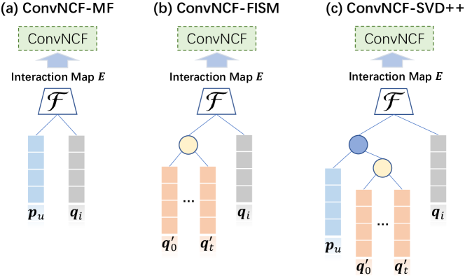
Figure 2. Illustration of the embedding function of the three ConvNCF methods.

MF adopts the simplest ID embedding function, i.e., directly projecting the ID of a user (an item) to latent vector representation:

(9) $$f^{U}(u)=\textbf{p}_{u},\quad f^{I}(i)=\textbf{q}_{i}.$$

Let the user embedding matrix be $\textbf{P}\in\mathbb{R}^{M\times K}$ and the item embedding matrix be $\textbf{Q}\in\mathbb{R}^{N\times K}$. This function is equal to taking out the $u$-th row of P as $u$’s embedding vector (i.e., $\textbf{p}_{u}$) and the $i$-th row of Q as $i$’s embedding vector (i.e., $\textbf{q}_{i}$).

In MF, each user is associated with an individualized set of parameters to denote the user’s interest — even two users have exactly the same interactions on items, they are parameterized differently in the model. As such, it is also called as user-based CF in recommendation literature. The problem of this setting is that, if a user has never been seen in the training set (i.e., cold-start), the model cannot obtain her embedding in the online phase, even though the user has some new interactions on items. In other words, the model lacks the ability to provide real-time personalization. Next, we introduce the setting of item-based CF, we can address this deficiency.

5.2. ConvNCF-FISM

Instead of directly projecting user ID to embedding vector, FISM represents a user with her historically interacted items, based on which the embedding function is defined:

(10) $$f^{U}(u)=\frac{1}{|\mathcal{R}_{u}|^{\alpha}}\sum_{t\in\mathcal{R}_{u}\backslash\{i\}}\textbf{q}^{\prime}_{t},\quad f^{I}(i)=\textbf{q}_{i},$$

where $\mathcal{R}_{u}$ denotes the set of items interacted by $u$, $\textbf{q}^{\prime}_{t}$ denotes the embedding of historical item $t$ in constructing the user embedding function. Note that FISM has three considerations to ensure the embedding quality: 1) the historical item embedding $\textbf{q}^{\prime}_{t}$ used in user embedding function is different from target item embedding $\textbf{q}_{t}$ used in item embedding function, which can improve the model representation ability; 2) the target item $i$ is excluded to represent the user, i.e., the $\mathcal{R}_{u}\backslash\{i\}$ term, so as to avoid information leakage in training; 3) the coefficient $\frac{1}{|\mathcal{R}_{u}|^{\alpha}}$ is to normalize users of different activity levels (by convention we set $\alpha$ as 0.5).

In FISM, a user’s embedding is aggregated from the embeddings of the user’s historically interacted items. Thus, for two users with the same interactions on items, their embeddings are the same. For a cold-start user, as long as she has new interactions, we can obtain her embedding instantaneously by calling the embedding function without re-training the model. Therefore, such item-based CF scheme is suitable to provide real-time personalization to refresh the recommendation for users that have new interactions.

5.3. ConvNCF-SVD++

SVD++ is a hybrid method that combines the user embedding design of MF and FISM. It uses both the ID and historically interacted items to represent a user, and defines the embedding function as:

(11) $$f^{U}(u)=\textbf{p}_{u}+\frac{1}{|\mathcal{R}_{u}|^{\alpha}}\sum_{t\in\mathcal{R}_{u}\backslash\{i\}}\textbf{q}^{\prime}_{t},\quad f^{I}(i)=\textbf{q}_{i},$$

where the notations follow the ones used in Equation (9) and (10). The user embedding function of SVD++ is the sum of the user embedding functions of MF and FISM, unifing the strengths of both methods. Specifically, $\textbf{p}_{u}$ is a static vector to encode user inherent preference, and $\sum_{t\in\mathcal{R}_{u}\backslash\{i\}}\textbf{q}^{\prime}_{t}$ can be dynamically adjusted by including recently interacted items. Note that SVD++ is a very competitive CF model that is known as the best single model in the Netflix Challenge (Bennett et al., 2007). By plugging its embedding functions into ConvNCF, we can further advance its performance.

5.4. Embedding Pre-training and Adaptive Regularization

Due to the multi-layer design of ConvNCF, the initialization of model parameters has a large impact on model training and its testing performance. As the convolutional layers are learned on the outer product of embeddings to generate the features used for prediction, a good initialization on embeddings is beneficial to the overall model learning. Thus, we propose to pre-train the embedding layer. For the three ConvNCF methods, we first train its shallow model counterpart, i.e., MF, FISM, and SVD++ for ConvNCF-MF, ConvNCF-FISM, and ConvNCF-SVD++, respectively. We then use the learned embeddings to initialize the embedding layer of the corresponding method. Our empirical studies find that this strategy can substantially improve the model performance.

After pre-training the embedding layer, we start training the ConvNCF model. As other model parameters are randomly initialized, the overall model is in an underfitting state. Thus, we disable regularization for the 1st epoch to make the model learn to fit the data as quickly as possible. For the following epochs, we enforce regularization on ConvNCF to prevent overfitting, including the $L_{2}$ regularization on the embedding layer (controlled by $\lambda_{1}$ and $\lambda_{2}$), convolution layers (controlled by $\lambda_{3}$), and the output layer (controlled by $\lambda_{4}$). It is worth noting that the regularization coefficients (especially $\lambda_{4}$ on the output layer) have a very large impact and should be carefully tuned for an optimal performance.

Table 3. Top-$k$ recommendation performance where $k\in\{5,10,20\}$. RI indicates the average improvement of ConvNCF-SVD++ over the baseline. ^∗ indicates that the improvements over all baselines are statistically significant for $p<0.05$.

Dataset	Model Type	Model	HR@$k$			NDCG@$k$			RI
			$k=5$	$k=10$	$k=20$	$k=5$	$k=10$	$k=20$
Gowalla	Popularity	ItemPop	0.2003	0.2785	0.3739	0.1099	0.1350	0.1591	+263.2%
	Linear Models	MF-BPR	0.6284	0.7480	0.8422	0.4825	0.5214	0.5454	+9.5%
		FISM	0.6170	0.7381	0.8347	0.4742	0.5135	0.5381	+11.1%
		SVD++	0.6545	0.7634	0.8475	0.5111	0.5465	0.5679	+5.6%
	Neural Network Models	MLP	0.6359	0.7590	0.8535	0.4802	0.5202	0.5443	+9.0%
		JRL	0.6685	0.7747	0.8561	0.5270	0.5615	0.5821	+3.4%
		NeuMF	0.6744	0.7793	0.8602	0.5319	0.5660	0.5865	+2.6%
	Our Models	ConvNCF-MF	0.6914	0.7936∗	0.8695∗	0.5494	0.5826	0.6019	-
		ConvNCF-FISM	0.6716	0.7767	0.8572	0.5312	0.5654	0.5859	-
		ConvNCF-SVD++	0.6949∗	0.7930	0.8657	0.5532∗	0.5851∗	0.6036∗	-
Yelp	Popularity	ItemPop	0.0710	0.1147	0.1732	0.0365	0.0505	0.0652	+197.0%
	Linear Models	MF-BPR	0.1752	0.2817	0.4203	0.1104	0.1447	0.1796	+11.2%
		FISM	0.1852	0.2884	0.4262	0.1174	0.1505	0.1852	+7.1%
		SVD++	0.1893	0.2998	0.4360	0.1208	0.1562	0.1905	+4.0%
	Neural Network Models	MLP	0.1766	0.2831	0.4203	0.1103	0.1446	0.1792	+11.1%
		JRL	0.1858	0.2922	0.4343	0.1177	0.1519	0.1877	+6.0%
		NeuMF	0.1881	0.2958	0.4385	0.1189	0.1536	0.1895	+4.9%
	Our Models	ConvNCF-MF	0.1978	0.3086	0.4430	0.1243	0.1600	0.1939	-
		ConvNCF-FISM	0.1925	0.3028	0.4423	0.1243	0.1598	0.1949	-
		ConvNCF-SVD++	0.1991∗	0.3092∗	0.4457∗	0.1275∗	0.1629∗	0.1973∗	-

6. Experiments

To evaluate our proposal, we conduct experiments to answer the following research questions:

RQ1:

How do our ConvNCF perform compared with state-of-the-art recommendation methods?

RQ2:

How do the embedding dimension correlations (captured by the outer product layer and convolution layers) contribute to the model performance?

RQ3:

How do the key hyper-parameters (e.g., feature maps and pre-training) affect ConvNCF’s performance?

6.1. Experimental Settings

Data Description

We conduct experiments on two publicly accessible datasets: Yelp and Gowalla.

Yelp. This is the Yelp Challenge data for user ratings on businesses. We filter the dataset same as (He et al., 2016a). Moreover, we merge the repetitive ratings at different timestamps to the earliest one, so as to study the performance of recommending novel items to a user. The final dataset obtains 25,815 users, 25,677 items, and 730,791 ratings.

Gowalla. This is the check-in dataset from Gowalla, a location-based social network, constructed by (Liang et al., 2016) for item recommendation. To ensure the quality of the dataset, we perform a modest filtering on the data, retaining users with at least two interactions and items with at least ten interactions. The final dataset contains 54,156 users, 52,400 items, and 1,249,703 interactions.

Evaluation Protocols

For each user in the dataset, we holdout the latest one interaction as the testing positive sample, and then pair it with $999$ items that the user did not rate before as the negative samples. Each method then generates predictions for these $1,000$ user-item pairs. To evaluate the results, we adopt two metrics Hit Ratio (HR) and Normalized Discounted Cumulative Gain (NDCG), same as (He et al., 2017). HR@$k$ is a recall-based metric, measuring whether the testing item is in the top-$k$ position (1 for yes and 0 otherwise). NDCG@$k$ assigns higher scores to the items within the top $k$ positions of the ranking list. To eliminate the effect of random oscillation, we report the average scores of the last ten epochs upon convergence.

Baselines

To justify the effectiveness of our method, we compare with the following methods:

ItemPop:

ranks the items based on their popularity, which is calculated by the number of interactions. It is always taken as a benchmark for recommender algorithms.

MF-BPR (Rendle et al., 2009):

optimizes the matrix factorization model with the pairwise BPR ranking loss. It is a competitive user-based CF method.

FISM (Kabbur et al., 2013):

replaces the user ID embedding with the item-based embedding function of Equation 10. It is a competitive item-based CF method.

SVD++ (Koren, 2008):

combines the user embedding design of MF and FISM, as formulated in 11. It is a strong CF model that scores the best single model in the Netflix challenge.

MLP (He et al., 2017):

is a NCF method that feeds the concatenation of user embedding and item embedding into the standard MLP for learning the interaction function. As no interaction between user embedding and item embedding is explicitly modeled, this model can be inferior to the MF model (He et al., 2017).

JRL (Zhang et al., 2017):

is a NCF method that places a MLP above the element-wise product of user embedding and item embedding. It enhances GMF (He et al., 2017) by placing multiple hidden layers above the element-wise product, while GMF directly outputs the prediction score from the element-wise product.

NeuMF (He et al., 2017):

is a state-of-the-art method for item recommendation, which ensembles GMF and MLP to learn the user-item interaction function.

The architecture of ConvNCF is shown in Figure 1. Above the outer product layer, there are six convolutional layers. Each of them has $32$ convolutional kernels with stride 2 and no padding. We implement the three ConvNCF methods as introduced in Section 5, which have the same architecture setting with difference only in the user embedding function.

Parameter Settings

Our methods are implemented in Tensorflow. We randomly holdout 1 training interaction for each user as the validation set to tune hyper-parameters. For a fair comparison, all models apply the same setting in terms of the model size and optimization: the embedding size is set to 64 and all models are optimized with the BPR loss using mini-batch Adagrad. For MLP, JRL, and NeuMF that have multiple fully connected layers, we tuned the number of layers from 1 to 3 following the tower structure of (He et al., 2017). For all models besides MF, we pre-train their embedding layers using MF embeddings, and the $L_{2}$ regularization for each method has been fairly tuned.

Due to the strong representation ability of ConvNCF, it is prone to overfitting. As such, tuning the regularization has a large impact on its performance. We divide the parameters of ConvNCF into two groups: embedding parameters ($\Theta_{U}$ and $\Theta_{I}$) and CNN parameters ($\Theta_{CNN}$ and w), and tune the regularization coefficient and learning rate separately for the two groups. For the embedding parameters, the optimal learning rate (under Adagrad) is around $0.001$ and $0.005$, and the regularization coefficients (i.e., $\lambda_{1}$, $\lambda_{2}$) are searched in $[0,10^{-7},10^{-6}]$. For the CNN parameters, the optimal learning rate is around 0.01 and 0.05, and the regularization coefficients (i.e., $\lambda_{3}$, $\lambda_{4}$) are searched in $[10^{-2},10^{-1},1,10]$.

6.2. Performance Comparison (RQ1)

Table 3 shows the Top-$k$ recommendation performance on both datasets where $k$ is set to 5, 10, and 20. We have the following key observations:

• Our ConvNCF methods achieve the best performance in general, and obtain high improvements over the compared methods. Particularly, each ConvNCF instantiation outperforms its linear counterpart in all settings (e.g., ConvNCF-MF vs. MF, ConvNCF-FISM vs. FISM). This justifies the utility of our ConvNCF design — using outer product (and CNN) to capture second-order (and high-order) correlations among embedding dimensions.

• Among the three ConvNCF methods, ConvNCF-SVD++ is the strongest and achieves the best performance in most settings. This demonstrates the utility of designing better embedding function for ConvNCF. Moreover, we find that ConvNCF-FISM achieves weak performance on Gowalla. We hypothesize the reason is that the item-based user representation mechanism does not work well for the Gowalla dataset, since FISM also underperforms MF substantially on Gowalla. Another obsrevation is that initialized with the pretrained embeddings, ConvNCF would significantly improve the performances in few epochs (Figure 3). In such few epochs, the embeddings would not change much, that implies that modeling the embedding correlations plays a significant role for the state-of-the-art performances.

• JRL consistently outperforms MLP by a large margin on both datasets. This indicates that, explicitly modeling the correlations of embedding dimensions is rather helpful for the followup learning of the hidden layers, even modeling the simple correlations that assume the dimensions are independent. Meanwhile, it also reveals the practical difficulties to train MLP well, although it has strong representation ability in principle (Hornik, 1991).

• The relatively weak performances of MF and FISM reflect that simple inner product of the user and item embeddings is far insufficient to depict the complex patterns within the user-item interactions. Moreover, MF outperforms FISM on Gowalla but underperforms FISM on Yelp. This implies that which embedding function works better is dependent on the properties of the dataset. Lastly, ItemPop achieves the worst performance, verifying the importance of considering users’ personalized preferences in the recommendation.

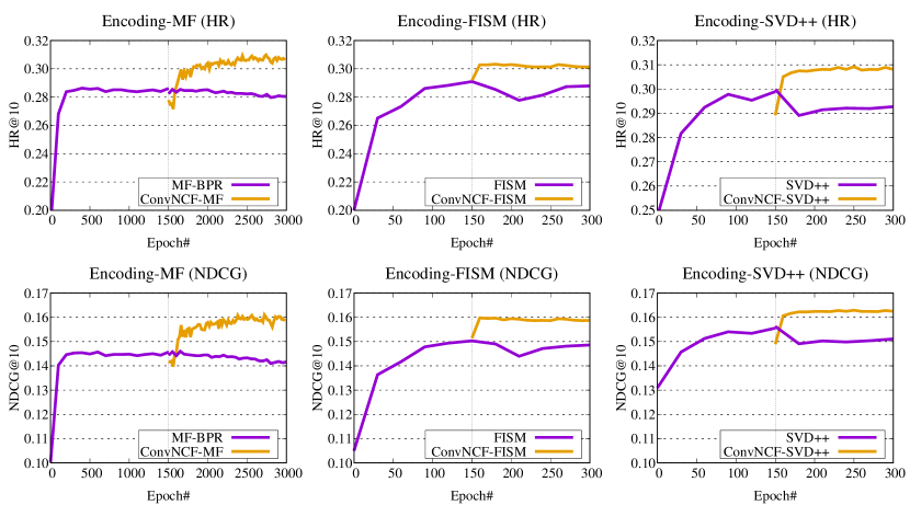
Figure 3. HR@10 and NDCG@10 of ConvNCF models and corresponding embedding models (i.e., MF-BPR (Rendle et al., 2009), SVD++ (Koren, 2008) and FISM (Kabbur et al., 2013)) on Yelp. The results verify that ConvNCF could effectively discover the inherent correlations between embedding dimensions.

6.3. Modeling Embedding Dimension Correlations (RQ2)

Through overall performance comparison, we have shown the strength of ConvNCF. Next, we conduct more experiments to verify the utility of modeling embedding dimension correlations, more concretely, the efficacy of outer product and CNN in ConvNCF. We choose ConvNCF-MF as an example to demonstrate the usefulness of outer product (for brevity, we term it as ConvNCF in this subsection only).

6.3.1. Efficacy of Outer Product

Besides outer product, another two choices that are commonly used in previous work are concatenation and element-wise product. It is worth mentioning that element-wise product, concatenation, and outer product operations have essentially different structures, since the outer product operation is performed based on a matrix while the other two operations are performed based on vectors. To conduct a fair evaluation, we implement the state-of-the-art models representing element-wise product and the concatenation style learning methods according to  (Zhang et al., 2017; He et al., 2017). As such, we compare the training progress of ConvNCF with GMF and JRL (which use element-wise product), and MLP (which uses concatenation). As can be seen from Figure 4, ConvNCF outperforms other methods by a large margin on both datasets, verifying the positive effect of using outer product above the embedding layer. Specifically, the improvements over GMF and JRL demonstrate that explicitly modeling the correlations between different embedding dimensions are useful. Lastly, the rather weak and unstable performance of MLP imply the difficulties to train MLP well, especially when the low-level has fewer semantics about the feature interactions. This is consistent with the recent finding of (He and Chua, 2017) in using MLP for sparse data prediction.

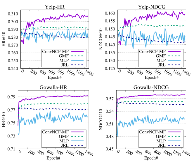
Figure 4. HR@10 and NDCG@10 of applying different operations above the embedding layer in each epoch (GMF and JRL use element-wise product, MLP uses concatenation, and ConvNCF uses outer product).

6.3.2. Efficacy of CNN

In order to verify the effectiveness of CNN over MLP, we make a fair comparison by training them based on the same 2D interaction map. Specifically, we first flatten the interaction map as a $K^{2}$ dimensional vector, and then place a 3-layer MLP above it. We term this method as ONCF-mlp. Figure 5 compares its performance with ConvNCF in each epoch. We can see that ONCF-mlp performs much worse than ConvNCF, in spite of the fact that it uses much more parameters (1000 times more) than ConvNCF. Another drawback of using such many parameters in ONCF-mlp is that it makes the model rather unstable, which is evidenced by its large variance in epoch. In contrast, our ConvNCF achieves much better and stable performance by using the locally connected CNN. These empirical evidence provide support for our motivation of designing ConvNCF and our discussion of MLP’s drawbacks in Section 4.3.1.

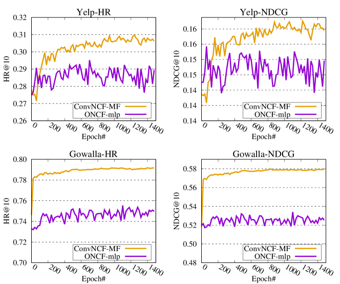
Figure 5. HR@10 and NDCG@10 of using different hidden layers above the interaction map (ConvNCF uses a 6-layer CNN and ONCF-mlp uses a 3-layer MLP).

6.4. Hyperparameter Study (RQ3)

6.4.1. Impact of Feature Map Number

The number of feature maps in each CNN layer affects the representation ability of our ConvNCF. Figure 6 shows the performance of ConvNCF-MF with respect to different numbers of feature maps. We can see that all the curves increase steadily and finally achieve similar performance, though there are some slight differences on the convergence curve. This reflects the strong expressiveness and generalization of using CNN above the interaction map since dramatically increasing the number of parameters of a neural network does not lead to overfitting. Consequently, our model is very suitable for practical use.

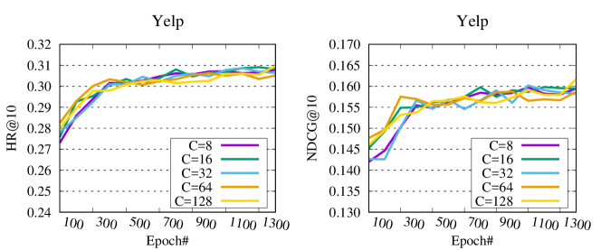
Figure 6. Performance of ConvNCF-MF w.r.t. different numbers of feature maps per convolutional layer (denoted by $C$) in each epoch on Yelp.

6.4.2. Pretraining on Embeddings.

In our experiments, all the embeddings used in ConvNCF are initialized by the pretrained parameters. We here compare the effect of training with pretraining and training from scratch. As shown in Figure 7, there are two curves. The orange one indicates the performance training with pretraining, and the purple one indicates the performance training from scratch. The orange curve at the left side of the dashed line presents the status pretraining the models and the rest presents the status training ConvNCF. Due to the simplicity of original models, the pretraining processs increase the performances soon. Based on these embeddings, ConvNCF obtains the state-of-the-art performance, which re-emphasizes the importance of modeling the dimension correlations. In contrast, training from scratch also grasps some information but due to more complex structure, it requires more efforts to achieve the nice performance.

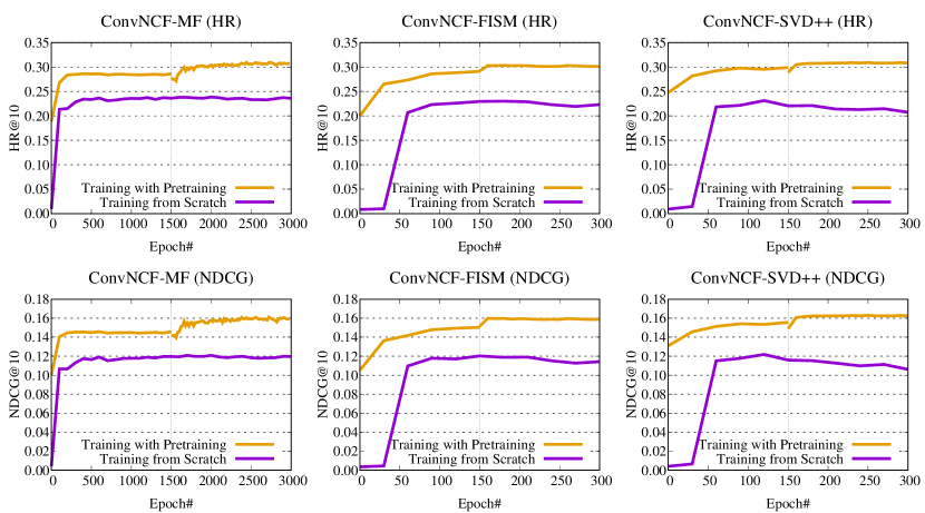
Figure 7. HR@10 and NDCG@10 on Yelp via different training tricks: training from scratch and training with pretraining. The results demonstrate that pretraining the embeddings with original models is helpful to efficiently obtain the well-performed ConvNCF.

7. Conclusion

In this paper, we presented a new neural network framework ConvNCF for collaborative filtering by modeling the embedding dimension correlations. Moreover, we proposed three variants of ConvNCF. ConvNCF is able to capture latent relations between embedding dimensions via the outer product operation. To learn more accurate preference, we used multiple convolution layers on top of the interaction map. Extensive experiments on two real-world datasets demonstrated that modeling the embedding dimension correlations was helpful for CF tasks. We further showed that ConvNCF outperforms state-of-the-art methods in the top-$k$ item recommendation task.

In future, we will explore more advanced CNN techniques such as attentive mechanism (Lin et al., 2017) and residual learning (He et al., 2016b) to learn higher-level representations. Moreover, we will extend ConvNCF to content-based recommendation scenarios (He and McAuley, 2016; Yu et al., 2018) since the item features have richer semantics than just an ID. Particularly, we are interested in building recommender systems for multimedia items like images and videos, and textual items like news.

- (1)
- Bai et al. (2017) Ting Bai, Ji-Rong Wen, Jun Zhang, and Wayne Xin Zhao. 2017. A Neural Collaborative Filtering Model with Interaction-based Neighborhood. In CIKM. 1979–1982.
- Bayer et al. (2017) Immanuel Bayer, Xiangnan He, Bhargav Kanagal, and Steffen Rendle. 2017. A Generic Coordinate Descent Framework for Learning from Implicit Feedback. In WWW. 1341–1350.
- Bennett et al. (2007) James Bennett, Stan Lanning, et al. 2007. The netflix prize. In Proceedings of KDD cup and workshop, Vol. 2007. New York, NY, USA, 35.
- Beutel et al. (2018) Alex Beutel, Paul Covington, Sagar Jain, Can Xu, Jia Li, Vince Gatto, and Ed H. Chi. 2018. Latent Cross: Making Use of Context in Recurrent Recommender Systems. In WSDM. 46–54.
- Cao et al. (2017a) Da Cao, Xiangnan He, Liqiang Nie, Xiaochi Wei, Xia Hu, Shunxiang Wu, and Tat-Seng Chua. 2017a. Cross-Platform App Recommendation by Jointly Modeling Ratings and Texts. ACM Transactions on Information Systems 35, 4 (July 2017), 37:1–37:27.
- Cao et al. (2017b) Da Cao, Liqiang Nie, Xiangnan He, Xiaochi Wei, Shunzhi Zhu, and Tat-Seng Chua. 2017b. Embedding factorization models for jointly recommending items and user generated lists. In SIGIR. ACM, 585–594.
- Chen et al. (2017) Jingyuan Chen, Hanwang Zhang, Xiangnan He, Liqiang Nie, Wei Liu, and Tat-Seng Chua. 2017. Attentive Collaborative Filtering: Multimedia Recommendation with Item- and Component-Level Attention. In SIGIR. 335–344.
- Chen et al. (2012) Tianqi Chen, Weinan Zhang, Qiuxia Lu, Kailong Chen, Zhao Zheng, and Yong Yu. 2012. SVDFeature: a toolkit for feature-based collaborative filtering. Journal of Machine Learning Research 13, Dec (2012), 3619–3622.
- Chen et al. (2018) Xu Chen, Yongfeng Zhang, Hongteng Xu, Zheng Qin, and Hongyuan Zha. 2018. Adversarial Distillation for Efficient Recommendation with External Knowledge. ACM Transactions on Information Systems (TOIS) 37, 1 (2018), 12.
- Cheng et al. (2019) Zhiyong Cheng, Xiaojun Chang, Lei Zhu, Rose C Kanjirathinkal, and Mohan Kankanhalli. 2019. MMALFM: Explainable recommendation by leveraging reviews and images. ACM Transactions on Information Systems (TOIS) 37, 2 (2019), 16.
- Cheng et al. (2018) Zhiyong Cheng, Ying Ding, Xiangnan He, Lei Zhu, Xuemeng Song, and Mohan S Kankanhalli. 2018. A^ 3NCF: An Adaptive Aspect Attention Model for Rating Prediction.. In IJCAI. 3748–3754.
- Cheng et al. (2017) Zhiyong Cheng, Jialie Shen, Lei Zhu, Mohan S Kankanhalli, and Liqiang Nie. 2017. Exploiting Music Play Sequence for Music Recommendation.. In IJCAI. 3654–3660.
- Covington et al. (2016) Paul Covington, Jay Adams, and Emre Sargin. 2016. Deep Neural Networks for YouTube Recommendations. In RecSys. 191–198.
- Cybenko (1989) George Cybenko. 1989. Approximation by superpositions of a sigmoidal function. Mathematics of control, signals and systems 2, 4 (1989), 303–314.
- Deng et al. (2017) Shuiguang Deng, Longtao Huang, Guandong Xu, Xindong Wu, and Zhaohui Wu. 2017. On deep learning for trust-aware recommendations in social networks. IEEE transactions on neural networks and learning systems 28, 5 (2017), 1164–1177.
- Ding et al. (2018) Jingtao Ding, Fuli Feng, Xiangnan He, Guanghui Yu, Yong Li, and Depeng Jin. 2018. An Improved Sampler for Bayesian Personalized Ranking by Leveraging View Data. In WWW. 13–14.
- Feng and Chua (2019) Xiangnan He Xiang Wang Cheng Luo Yiqun Liu Feng, Fuli and Tat-Seng Chua. 2019. Temporal Relational Ranking for Stock Prediction. ACM Transactions on Information Systems (TOIS) 37, 2 (2019), 27.
- Gardner and Dorling (1998) Matt W Gardner and SR Dorling. 1998. Artificial neural networks (the multilayer perceptron)-a review of applications in the atmospheric sciences. Atmospheric environment 32, 14-15 (1998), 2627–2636.
- Gomez-Uribe and Hunt (2016) Carlos A Gomez-Uribe and Neil Hunt. 2016. The netflix recommender system: Algorithms, business value, and innovation. ACM Transactions on Management Information Systems (TMIS) 6, 4 (2016), 13.
- Guan et al. (2019) Xinyu Guan, Zhiyong Cheng, Xiangnan He, Yongfeng Zhang, Zhibo Zhu, Qinke Peng, and Tat-Seng Chua. 2019. Attentive Aspect Modeling for Review-aware Recommendation. ACM Transactions on Information Systems (TOIS) 37, 3 (2019), 28.
- Guo et al. (2019) Yangyang Guo, Zhiyong Cheng, Liqiang Nie, Yinglong Wang, Jun Ma, and Mohan Kankanhalli. 2019. Attentive Long Short-Term Preference Modeling for Personalized Product Search. ACM Transactions on Information Systems (TOIS) 37, 2 (2019), 19.
- He et al. (2016b) Kaiming He, Xiangyu Zhang, Shaoqing Ren, and Jian Sun. 2016b. Deep residual learning for image recognition. In CVPR. 770–778.
- He and McAuley (2016) Ruining He and Julian McAuley. 2016. VBPR: Visual Bayesian Personalized Ranking from Implicit Feedback.. In AAAI. 144–150.
- He and Chua (2017) Xiangnan He and Tat-Seng Chua. 2017. Neural factorization machines for sparse predictive analytics. In SIGIR. 355–364.
- He et al. (2018a) Xiangnan He, Xiaoyu Du, Xiang Wang, Feng Tian, Jinhui Tang, and Tat-Seng Chua. 2018a. Outer Product-based Neural Collaborative Filtering. In IJCAI.
- He et al. (2018b) Xiangnan He, Zhankui He, Xiaoyu Du, and Tat-Seng Chua. 2018b. Adversarial Personalized Ranking for Item Recommendation. In SIGIR.
- He et al. (2018c) Xiangnan He, Zhenkui He, Jingkuan Song, Zhenguang Liu, Yu-Gang Jiang, and Tat-Seng Chua. 2018c. NAIS: Neural Attentive Item Similarity Model for Recommendation. IEEE Transactions on Knowledge and Data Engineering (2018).
- He et al. (2017) Xiangnan He, Lizi Liao, Hanwang Zhang, Liqiang Nie, Xia Hu, and Tat-Seng Chua. 2017. Neural collaborative filtering. In WWW. 173–182.
- He et al. (2019) Xiangnan He, Jinhui Tang, Xiaoyu Du, Richang Hong, Tongwei Ren, and Tat-Seng Chua. 2019. Fast Matrix Factorization with Non-Uniform Weights on Missing Data. IEEE transactions on neural networks and learning systems (2019).
- He et al. (2016a) Xiangnan He, Hanwang Zhang, Min-Yen Kan, and Tat-Seng Chua. 2016a. Fast matrix factorization for online recommendation with implicit feedback. In SIGIR. 549–558.
- Hochreiter and Schmidhuber (1997) Sepp Hochreiter and Jürgen Schmidhuber. 1997. Long short-term memory. Neural computation 9, 8 (1997), 1735–1780.
- Hornik (1991) Kurt Hornik. 1991. Approximation capabilities of multilayer feedforward networks. Neural networks 4, 2 (1991), 251–257.
- Hsieh et al. (2017) Cheng-Kang Hsieh, Longqi Yang, Yin Cui, Tsung-Yi Lin, Serge Belongie, and Deborah Estrin. 2017. Collaborative metric learning. In WWW. 193–201.
- Huang et al. (2017) Gao Huang, Zhuang Liu, Kilian Q Weinberger, and Laurens van der Maaten. 2017. Densely connected convolutional networks. In CVPR. 4700–4708.
- Kabbur et al. (2013) Santosh Kabbur, Xia Ning, and George Karypis. 2013. Fism: factored item similarity models for top-n recommender systems. In SIGKDD. ACM, 659–667.
- Kim et al. (2016) Donghyun Kim, Chanyoung Park, Jinoh Oh, Sungyoung Lee, and Hwanjo Yu. 2016. Convolutional matrix factorization for document context-aware recommendation. In RecSys. ACM, 233–240.
- Koren (2008) Yehuda Koren. 2008. Factorization meets the neighborhood: a multifaceted collaborative filtering model. In SIGKDD. ACM, 426–434.
- Koren et al. (2009) Yehuda Koren, Robert Bell, and Chris Volinsky. 2009. Matrix factorization techniques for recommender systems. Computer 42, 8 (2009).
- Krizhevsky et al. (2012) Alex Krizhevsky, Ilya Sutskever, and Geoffrey E Hinton. 2012. Imagenet classification with deep convolutional neural networks. In NIPS. 1097–1105.
- Liang et al. (2016) Dawen Liang, Laurent Charlin, James McInerney, and David M Blei. 2016. Modeling user exposure in recommendation. In WWW. 951–961.
- Lin et al. (2017) Zhouhan Lin, Minwei Feng, Cicero Nogueira dos Santos, Mo Yu, Bing Xiang, Bowen Zhou, and Yoshua Bengio. 2017. A structured self-attentive sentence embedding. In ICLR.
- Lu et al. (2015) Zhongqi Lu, Zhicheng Dou, Jianxun Lian, Xing Xie, and Qiang Yang. 2015. Content-Based Collaborative Filtering for News Topic Recommendation.. In AAAI. 217–223.
- Luo et al. (2016) Xin Luo, MengChu Zhou, Shuai Li, Zhuhong You, Yunni Xia, and Qingsheng Zhu. 2016. A nonnegative latent factor model for large-scale sparse matrices in recommender systems via alternating direction method. IEEE transactions on neural networks and learning systems 27, 3 (2016), 579–592.
- Ma et al. (2018a) Zhanyu Ma, Yuping Lai, W Bastiaan Kleijn, Yi-Zhe Song, Liang Wang, and Jun Guo. 2018a. Variational Bayesian learning for Dirichlet process mixture of inverted Dirichlet distributions in non-Gaussian image feature modeling. IEEE transactions on neural networks and learning systems 99 (2018), 1–15.
- Ma et al. (2018b) Zhanyu Ma, Jing-Hao Xue, Arne Leijon, Zheng-Hua Tan, Zhen Yang, and Jun Guo. 2018b. Decorrelation of neutral vector variables: Theory and applications. IEEE transactions on neural networks and learning systems 29, 1 (2018), 129–143.
- Pan et al. (2019) Weike Pan, Qiang Yang, Wanling Cai, Yaofeng Chen, Qing Zhang, Xiaogang Peng, and Zhong Ming. 2019. Transfer to rank for heterogeneous one-class collaborative filtering. ACM Transactions on Information Systems (TOIS) 37, 1 (2019), 10.
- Qian et al. (2019) Tieyun Qian, Bei Liu, Quoc Viet Hung Nguyen, and Hongzhi Yin. 2019. Spatiotemporal representation learning for translation-based poi recommendation. ACM Transactions on Information Systems (TOIS) 37, 2 (2019), 18.
- Qu and He (2018) Bohui Fang Weinan Zhang Ruiming Tang Minzhe Niu Huifeng Guo Yong Yu Qu, Yanru and Xiuqiang He. 2018. Product-Based Neural Networks for User Response Prediction over Multi-Field Categorical Data. ACM Transactions on Information Systems (TOIS) 37, 1 (2018), 5.
- Rendle (2010) Steffen Rendle. 2010. Factorization machines. In ICDM. 995–1000.
- Rendle et al. (2009) Steffen Rendle, Christoph Freudenthaler, Zeno Gantner, and Lars Schmidt-Thieme. 2009. BPR: Bayesian personalized ranking from implicit feedback. In UAI. 452–461.
- Sharma et al. (2015) Amit Sharma, Jake M Hofman, and Duncan J Watts. 2015. Estimating the causal impact of recommendation systems from observational data. In Proceedings of the Sixteenth ACM Conference on Economics and Computation. ACM, 453–470.
- Tay et al. (2018) Yi Tay, Luu Anh Tuan, and Siu Cheung Hui. 2018. Latent Relational Metric Learning via Memory-based Attention for Collaborative Ranking. In WWW. 729–739.
- Wang et al. (2018) Hongwei Wang, Fuzheng Zhang, Xing Xie, and Minyi Guo. 2018. DKN: Deep Knowledge-Aware Network for News Recommendation. In WWW. 1835–1844.
- Wang et al. (2015) Suhang Wang, Jiliang Tang, Yilin Wang, and Huan Liu. 2015. Exploring Implicit Hierarchical Structures for Recommender Systems. In IJCAI. 1813–1819.
- Wang et al. (2017) Xiang Wang, Xiangnan He, Liqiang Nie, and Tat-Seng Chua. 2017. Item silk road: Recommending items from information domains to social users. In SIGIR. 185–194.
- Wu et al. (2019) Libing Wu, Cong Quan, Chenliang Li, Qian Wang, Bolong Zheng, and Xiangyang Luo. 2019. A context-aware user-item representation learning for item recommendation. ACM Transactions on Information Systems (TOIS) 37, 2 (2019), 22.
- Wu et al. (2016) Yao Wu, Christopher DuBois, Alice X Zheng, and Martin Ester. 2016. Collaborative denoising auto-encoders for top-n recommender systems. In WSDM. ACM, 153–162.
- Xue et al. (2017) Hong-Jian Xue, Xinyu Dai, Jianbing Zhang, Shujian Huang, and Jiajun Chen. 2017. Deep Matrix Factorization Models for Recommender Systems. In IJCAI. 3203–3209.
- Yu and Koltun (2015) Fisher Yu and Vladlen Koltun. 2015. Multi-scale context aggregation by dilated convolutions. arXiv preprint arXiv:1511.07122 (2015).
- Yu et al. (2018) Wenhui Yu, Huidi Zhang, Xiangnan He, Xu Chen, Li Xiong, and Zheng Qin. 2018. Aesthetic-based Clothing Recommendation. In WWW. 649–658.
- Yuan et al. (2016) Fajie Yuan, Guibing Guo, Joemon M Jose, Long Chen, Haitao Yu, and Weinan Zhang. 2016. Lambdafm: learning optimal ranking with factorization machines using lambda surrogates. In CIKM. ACM, 227–236.
- Yuan et al. (2019) Fajie Yuan, Alexandros Karatzoglou, Ioannis Arapakis, Joemon M Jose, and Xiangnan He. 2019. A Simple Convolutional Generative Network for Next Item Recommendation. In WSDM.
- Yuan et al. (2018) Fajie Yuan, Xin Xin, Xiangnan He, Guibing Guo, Weinan Zhang, Chua Tat-Seng, and Joemon M Jose. 2018. fbgd: Learning embeddings from positive unlabeled data with bgd. (2018).
- Zhang et al. (2017) Yongfeng Zhang, Qingyao Ai, Xu Chen, and W Bruce Croft. 2017. Joint representation learning for top-n recommendation with heterogeneous information sources. In CIKM. 1449–1458.
- Zhang et al. (2013) Yongfeng Zhang, Min Zhang, Yiqun Liu, Shaoping Ma, and Shi Feng. 2013. Localized matrix factorization for recommendation based on matrix block diagonal forms. In Proceedings of the 22nd international conference on World Wide Web. ACM, 1511–1520.
- Zhao et al. (2018) Wayne Xin Zhao, Wenhui Zhang, Yulan He, Xing Xie, and Ji-Rong Wen. 2018. Automatically learning topics and difficulty levels of problems in online judge systems. ACM Transactions on Information Systems (TOIS) 36, 3 (2018), 27.
- Zhao et al. (2016) Zhou Zhao, Hanqing Lu, Deng Cai, Xiaofei He, and Yueting Zhuang. 2016. User preference learning for online social recommendation. IEEE Transactions on Knowledge and Data Engineering 28, 9 (2016), 2522–2534.