A morphology-independent search for gravitational wave echoes in data from the first and second observing runs of Advanced LIGO and Advanced Virgo

Abstract

Gravitational wave echoes have been proposed as a smoking-gun signature of exotic compact objects with near-horizon structure. Recently there have been observational claims that echoes are indeed present in stretches of data from Advanced LIGO and Advanced Virgo immediately following gravitational wave signals from presumed binary black hole mergers, as well as a binary neutron star merger. In this paper we deploy a morphology-independent search algorithm for echoes introduced in Tsang et al., Phys. Rev. D 98, 024023 (2018), which (a) is able to accurately reconstruct a possible echoes signal with minimal assumptions about their morphology, and (b) computes Bayesian evidences for the hypotheses that the data contain a signal, an instrumental glitch, or just stationary, Gaussian noise. Here we apply this analysis method to all the significant events in the first Gravitational Wave Transient Catalog (GWTC-1), which comprises the signals from binary black hole and binary neutron star coalescences found during the first and second observing runs of Advanced LIGO and Advanced Virgo. In all cases, the ratios of evidences for signal versus noise and signal versus glitch do not rise above their respective “background distributions” obtained from detector noise, the smallest $p$-value being 3% (for event GW170823). Hence we find no statistically significant evidence for echoes in GWTC-1.

Introduction. Over the past several years, the twin Advanced LIGO observatories Aasi et al. (2015) have been detecting gravitational wave (GW) signals from coalescences of compact binary objects on a regular basis Abbott (2017); Abbott et al. (2016a); Abbott et al. (2016b); Abbott et al. (2017a, b). Meanwhile Advanced Virgo Acernese et al. (2015) has joined the global network of detectors, leading to further detections, including a binary neutron star inspiral Abbott et al. (2017c). In the first and second observing runs a total of 11 detections were made, which are summarized in Abbott et al. (2018a); the latter reference will be referred to as GWTC-1 (for Gravitational Wave Transient Catalog 1).

Thanks to these observations, general relativity (GR) has been subjected to a range of tests. For the first time we had access to the genuinely strong-field dynamics of the theory Abbott (2017); Abbott et al. (2016c, b); Abbott et al. (2017a, 2018b). Possible dispersion of gravitational waves was strongly constrained, leading to stringent upper bounds on the mass of the graviton and on local Lorentz invariance violations Abbott et al. (2016c); Abbott et al. (2017a, 2018b). As a next step, we want to probe the nature of the compact objects themselves. Based on the available data, how certain can we be that the more massive compact objects that were observed were indeed the standard black holes of classical, vacuum general relativity? A variety of alternative objects (“black hole mimickers”) have been proposed; see e.g. Barack et al. (2018) for an overview. When such objects are part of a binary system that undergoes coalescence, anomalous effects associated with them can leave an imprint upon the observed gravitational wave signal, including tidal effects Cardoso et al. (2017); Johnson-Mcdaniel et al. (2018); dynamical friction as well as resonant excitations due to dark matter clouds surrounding the objects Baumann et al. (2019); violations of the no-hair conjecture Carullo et al. (2018); Brito et al. (2018); and finally through gravitational wave “echoes” that might follow a merger Cardoso et al. (2016a, b); Cardoso and Pani (2017); Cardoso et al. (2019).

In this paper we will in particular search for echoes. In the case of exotic compact objects that lack a horizon, ingoing gravitational waves (e.g. resulting from a merger) can reflect multiple times off effective radial potential barriers, with wave packets leaking out at set times and escaping to infinity. Given an exotic object with mass $M$ and a horizon modification with typical length scale $\ell$, the time between these echoes tends to be constant, and approximately equal to $\Delta t\simeq nM\log(M/\ell)$, with $n$ a factor that is determined by the nature of the object Cardoso et al. (2016b). Setting $\ell$ equal to the Planck length, for the masses involved in the binary coalescences of GWTC-1 one can expect $\Delta t$ to range from a few to a few hundred milliseconds.

In Abedi et al. (2017); Westerweck et al. (2017), searches for echoes were presented using a bank of template waveforms characterized by the above $\Delta t$ as well as a characteristic frequency, a damping factor, and a widening factor between successive echoes. Since then, template-based search methods were developed which explore the relevant parameter space in a more efficient way Lo et al. (2018); Nielsen et al. (2018), or use more sophisticated templates Uchikata et al. (2019). A potential drawback here is that echo waveforms have been explicitly calculated only for selected exotic objects under various assumptions Cardoso et al. (2016b); Cardoso and Pani (2017), and even then only in an exploratory way Mark et al. (2017). Hence it is desirable to have a method to search for and characterize generic echoes, irrespective of their detailed morphology. A model-independent search for echoes was presented in Abedi and Afshordi (2018), but essentially assuming that individual echoes can be approximated by Dirac delta functions. In Conklin et al. (2017) a search was performed by looking for coherent excess power in a succession of windows in time or frequency. In this paper we instead employ the framework developed in Tsang et al. (2018) based on the BayesWave algorithm Cornish and Littenberg (2015); Littenberg and Cornish (2015) which can be used to not only detect but also reconstruct and characterize echo signals of an a priori unknown form.

Method. The method we use was extensively described in Tsang et al. (2018); here we only give an overview and then describe how it was applied to data from GWTC-1. We model the detector data ${\bf s}$ as

$${\bf s}={\bf R}\ast{\bf h}+{\bf g}+{\bf n_{g}},$$ (1)

where ${\bf R}$ is the response of the network to gravitational waves, ${\bf h}$ is the potential signal that is coherent across the detectors, ${\bf g}$ denotes possible instrumental transients or glitches, and ${\bf n_{g}}$ is a contribution from stationary, Gaussian noise. The signal ${\bf h}$ and the glitches ${\bf g}$ can both be decomposed in terms of a set of basis functions, and Bayesian evidences can be obtained for the hypotheses that either are present in the data. An important difference between signals and glitches is that the former will be present in the data of all the detectors in a coherent way (taking into account the different antenna responses), whereas the latter will manifest themselves incoherently. If the data contain a coherent signal, then typically a smaller number of basis functions will be needed to reconstruct it than to reconstruct incoherent glitches, so that the glitch model incurs an Occam penalty. At the same time, a reconstruction of the shape of the signal is obtained from the corresponding superposition of basis functions. For our purposes a natural choice for the basis functions is a “train” of sine-Gaussians. Individual sine-Gaussians are characterized by an amplitude $A$, a central frequency $f_{0}$, a damping time $\tau$, and a reference phase $\phi_{0}$; the train of sine-Gaussians as a whole also involves a central time $t_{0}$ of the first sine-Gaussian, a time $\Delta t$ between successive sine-Gaussians, and in going from one sine-Gaussian to the next also a relative phase shift $\Delta\phi$, an amplitude damping factor $\gamma$, and a widening factor $w$. Although there is no expectation that real echoes signals would resemble any one of these “generalized wavelets”, it is reasonable to assume that superpositions of them will be able to catch a wide variety of physical echoes waveforms and, if the first few echoes are sufficiently loud, provide an adequate reconstruction. Finally, the noise model ${\bf n_{g}}$ consists of colored Gaussian noise, the power spectral density of which is computed using a combination of smooth spline curves and a collection of Lorentzians to fit sharp spectral lines Littenberg and Cornish (2015). For each of the three models, the relevant parameter space is sampled over using a reversible jump Markov chain Monte Carlo algorithm, in which the number of generalized wavelets is also allowed to vary freely. Evidences for the three hypotheses are estimated through thermodynamic integration, yielding Bayes factors $B_{S/N}$ and $B_{S/G}$ for, respectively, the signal versus noise and signal versus glitch models Cornish and Littenberg (2015). This allows us to not only perform model selection, but also to reconstruct and characterize the signal. The algorithm is also applied to many stretches of detector noise, leading to a background distribution for $B_{S/N}$ and $B_{S/G}$ which can then be used to assess the statistical significance of potential echoes signals in the usual way. For more details we refer to Tsang et al. (2018).

In analyzing the stretches of data immediately preceding the events in GWTC-1 (for background calculation) or immediately after them (to search for echoes), we need to choose priors. We take $f_{0}$ to be uniform in the interval $[30,1024]$ Hz (respectively the lower cut-off frequency and half the sampling rate of the analysis), and the quality factor $Q=2\pi f_{0}\tau\in[2,40]$ uniformly, so that $\tau$ takes values roughly between $3\times 10^{-4}$ s and $0.2$ s, consistent with time scales set by the masses involved in the events. We let $\phi_{0}$ be uniform in $[0,2\pi]$. The prior on $A$ is based on signal-to-noise ratio as in Cornish and Littenberg (2015). We take uniform priors $\Delta t\in[0,0.7]$ s, $\Delta\phi\in[0,2\pi]$, $\gamma\in[0,1]$, and $w\in[1,2]$. For definiteness, each generalized wavelet contains five sine-Gaussians. We also need to specify a prior for the central time of the first sine-Gaussian in a generalized wavelet. Here we want to start analyzing at a time that is safely beyond the plausible duration of the ringdown of the remnant object. Let $t_{\rm event}$ be the arrival time for a given binary coalescence event as given in Abbott et al. (2018a); then we take $t_{0}$ to be uniform in $[t_{\rm event}+4\tau_{220},t_{\rm event}+4\tau_{220}+0.5\,\mbox{s}]$. The value for $\tau_{220}$ is a conservatively long estimate for the decay time of the $220$ mode in the ringdown, using the fitting formula $\tau_{220}(M_{f},a_{f},z)$ of Berti et al. (2006), where for the final mass $M_{f}$, the final spin $a_{f}$, and the redshift $z$ we take values at the upper bounds of the 90% confidence intervals listed in Abbott et al. (2018a); typically this comes to a few milliseconds. We note that our choices for parameter prior ranges, though pertaining to generalized wavelet decompositions rather than waveform templates, include the corresponding values for $t_{0}$, $\gamma$, and $A$ at which the template-based analysis of Abedi et al. (2017) claimed tentative evidence for echoes related to GW150914, GW151012, and GW151226.

To construct background distributions for the log Bayes factors $\log B_{S/N}$ and $\log B_{S/G}$, we use stretches of data preceding each coalescence event in GWTC-1 in the following way. In the interval between 1050 s and 250 s before the GPS time of a binary coalescence trigger as given in Abbott et al. (2018a), we define 100 sub-intervals of 8 s each. (No signal in GWTC-1 will have been in the detectors’ sensitive frequency band for more than 250 s, hence these intervals should effectively contain noise only.) For each of these intervals we compute $\log B_{S/N}$ and $\log B_{S/G}$, where the priors for the parameters of the generalized wavelets are as explained above; the values for $t_{\rm event}$ are chosen to be at the start of each interval. The log Bayes factors from times preceding all the events that were seen in two detectors obtained in this way are put into histograms, and the same is done separately for log Bayes factors from times preceding all the 3-detector events. These histograms are normalized, and smoothened using Gaussian kernel density estimates to obtain approximate probability distributions for $\log B_{S/N}$ and $\log B_{S/G}$ in the absence of echoes signals.

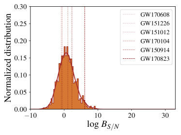
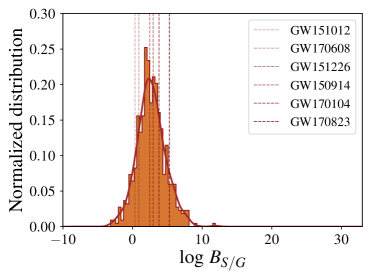
Figure 1: Background distributions (orange histograms, smoothened in brown) and foreground (vertical dashed lines, shaded by their values and labelled left to right) for the log Bayes factors for signal versus noise $\log B_{S/N}$ (top) and signal versus glitch $\log B_{S/G}$ (bottom), for the 2-detector events of GWTC-1. The associated $p$-values can be found in Table 1.

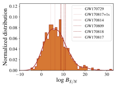
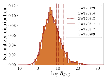
Figure 2: The same as in Fig. 1, but now for the 3-detector events of GWTC-1. The thin solid lines in each of the two panels are for an analysis of GW170817 in which the prior range for the time of the first echo was centered at 1.0 s after the event time, where Abedi and Afshordi (2018) claimed tentative evidence for an echo. For the associated $p$-values, see Table 2.

Event		$\log B_{S/N}$		$p_{S/N}$		$\log B_{S/G}$		$p_{S/G}$
GW150914		2.32		0.26		2.95		0.43
GW151012		-0.59		0.70		0.35		0.88
GW151226		-0.67		0.72		2.48		0.53
GW170104		1.09		0.44		3.80		0.28
GW170608		-0.90		0.75		0.90		0.82
GW170823		6.11		0.03		5.29		0.11
Combined				0.34				0.57

Table 1: Log Bayes factors for signal versus noise and signal versus glitch, and the corresponding $p$-values, for events seen in two detectors. The bottom row contains the combined $p$-values for all these events together.

Event		$\log B_{S/N}$		$p_{S/N}$		$\log B_{S/G}$		$p_{S/G}$
GW170729		4.24		0.67		5.64		0.62
GW170809		9.05		0.31		12.69		0.09
GW170814		8.75		0.33		8.54		0.34
GW170817		11.05		0.19		10.30		0.20
GW170817+1s		6.19		0.52		9.39		0.27
GW170818		10.39		0.23		9.36		0.27
Combined				0.47				0.22

Table 2: The same as in Table 2, but now for the events that were seen in three detectors. In the case of GW170817 we also include results for which the prior range for the time of the first echo was centered at 1.0 s after the event time, where Abedi and Afshordi (2018) claimed tentative evidence for an echo. The combined $p$-values take the latter prior choice for this particular event.

Finally, we calculate log Bayes factors for times following the coalescence events of GWTC-1, using the same priors, but now setting $t_{\rm event}$ to the arrival times for the events given in Abbott et al. (2018a). Considering $\log B_{S/N}$ or $\log B_{S/G}$ and the relevant number of detectors, the normalized, smoothened background distributions $\mathcal{P}(\log B)$ are used to compute $p$-values:

$$p=1-\int_{-\infty}^{\log B}\mathcal{P}(x)\,dx.$$ (2)

Combined $p$-values from all the events are obtained using Fisher’s prescription Fisher (1970). Given individual $p$-values $p_{i}$, $i=1,\ldots,N$, one defines

$$S=-2\sum_{i=1}^{N}\log(p_{i}),$$ (3)

and the combined $p$-value is calculated as

$$p_{\rm comb}=1-\int_{0}^{S}\chi^{2}_{2N}(x)\,dx,$$ (4)

where $\chi^{2}_{2N}$ is the chi-squared distribution with $2N$ degrees of freedom.

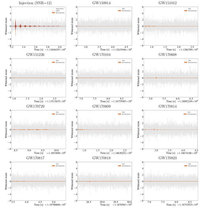
Figure 3: Stretches of whitened data (gray) and signal reconstructions (red) for a simulated echoes signal as described in the main text (top left panel) and for data immediately after the events in GWTC-1. In the case of GW170817, the first echo is searched for in an interval centered at 1.0 s after the event time. In all cases the event GPS time corresponds to the left bound of the panel.

Results and discussion. Figures 1 and 2 show background and foreground for $\log B_{S/N}$ and $\log B_{S/G}$ in the case of, respectively, 2-detector and 3-detector signals, and in Tables 1 and 2 we list the specific log Bayes factors for these cases, as well as associated $p$-values. All foreground results are in the support of the relevant background distributions. For signal versus noise, the smallest $p$-value is 3% (the case of GW170823), whereas for signal versus glitch the $p$-values do not go below 9% (see GW170809). In summary, we find no statistically significant evidence for echoes in GWTC-1. For the binary black hole observations in particular, this statement is in agreement with the template-based searches in Westerweck et al. (2017); Nielsen et al. (2018); Uchikata et al. (2019). (Note that a quantitative comparison of $p$-values is hard to make, because of the very specific signal shapes that are assumed in the latter analyses.)

Our results in Fig. 2 and Table 2 include the binary neutron star inspiral GW170817, analyzed in the same manner as the binary black hole merger signals. In Abbott et al. (2019), an analysis using the original BayesWave algorithm of Cornish and Littenberg (2015); Littenberg and Cornish (2015) (i.e. employing wavelets that are simple sine-Gaussians) yielded no evidence for a post-merger signal. Using our generalized wavelets, we obtain $\log B_{S/N}=11.05$ and $\log B_{S/G}=10.30$, both consistent with background. Hence in particular we do not find evidence for an echoes-like post-merger signal either, at least not up to $\lesssim 0.5$ s after the event’s GPS time. In Abedi and Afshordi (2018), tentative evidence was claimed for echoes starting at $t_{0}=t_{\rm event}+1.0$ s. Re-analyzing with the same priors as above but this time $t_{0}\in[t_{\rm event}+0.75\,\mbox{s},t_{\rm event}+1.25\,\mbox{s}]$, we find $\log B_{S/N}=6.19$ and $\log B_{S/G}=9.39$, both of which are consistent with their respective background distributions. Hence also when the time of the first echo is in this time interval we find no significant evidence for echoes. That said, we explicitly note that in the case of a black hole resulting from a binary neutron star merger of total mass $\sim 2.7\,M_{\odot}$ Abbott et al. (2019), we expect the dominant ringdown frequency and hence the central frequency $f_{0}$ of the echoes to be above 6000 Hz, i.e. above our prior upper bound, but also much beyond the detectors’ frequency reach for plausible energies emitted Abbott et al. (2017d). Foreground and background analyses with a correspondingly high frequency range are left for future work.

Finally, in Fig. 3 we show signal reconstructions (medians and 90% credible intervals) in terms of generalized wavelets for all the GWTC-1 events. For illustration purposes we also include the reconstruction of a simulated echoes waveform following the inspiral of a particle in a Schwarzschild spacetime with Neumann reflective boundary conditions just outside of where the horizon would have been, at mass ratio $q=100$ Khanna and Price (2017); Price and Khanna (2017). The simulated signal was embedded into detector noise at a signal-to-noise ratio (SNR) of 12, roughly corresponding to the SNR in the ringdown part of GW150914, had it been observed with Advanced LIGO sensitivity of the second observing run. In all cases the whitened raw data is shown, along with the whitened signal reconstruction. We include these reconstructions for completeness; our main results are the ones in Figs. 1, 2 and Tables 1, 2. Nevertheless, the reconstruction plots are visually consistent with our core results.

References

- Aasi et al. (2015) J. Aasi et al. (LIGO Scientific), Class.Quant.Grav. 32, 074001 (2015), eprint 1411.4547.
- Abbott (2017) B. P. Abbott (2017), pp. 291–311.
- Abbott et al. (2016a) B. P. Abbott et al. (Virgo, LIGO Scientific), Phys. Rev. Lett. 116, 241103 (2016a), eprint 1606.04855.
- Abbott et al. (2016b) B. P. Abbott et al. (Virgo, LIGO Scientific), Phys. Rev. X6, 041015 (2016b), eprint 1606.04856.
- Abbott et al. (2017a) B. P. Abbott et al. (VIRGO, LIGO Scientific), Phys. Rev. Lett. 118, 221101 (2017a), eprint 1706.01812.
- Abbott et al. (2017b) B. P. Abbott et al. (Virgo, LIGO Scientific), Astrophys. J. 851, L35 (2017b), eprint 1711.05578.
- Acernese et al. (2015) F. Acernese et al. (Virgo), Class. Quant. Grav. 32, 024001 (2015), eprint 1408.3978.
- Abbott et al. (2017c) B. Abbott et al. (Virgo, LIGO Scientific), Phys. Rev. Lett. 119, 161101 (2017c), eprint 1710.05832.
- Abbott et al. (2018a) B. P. Abbott et al. (LIGO Scientific, Virgo) (2018a), eprint 1811.12907.
- Abbott et al. (2016c) B. P. Abbott et al. (Virgo, LIGO Scientific), Phys. Rev. Lett. 116, 221101 (2016c), eprint 1602.03841.
- Abbott et al. (2018b) B. P. Abbott et al. (LIGO Scientific, Virgo) (2018b), eprint 1811.00364.
- Barack et al. (2018) L. Barack et al. (2018), eprint 1806.05195.
- Cardoso et al. (2017) V. Cardoso, E. Franzin, A. Maselli, P. Pani, and G. Raposo, Phys. Rev. D95, 084014 (2017), [Addendum: Phys. Rev.D95,no.8,089901(2017)], eprint 1701.01116.
- Johnson-Mcdaniel et al. (2018) N. K. Johnson-Mcdaniel, A. Mukherjee, R. Kashyap, P. Ajith, W. Del Pozzo, and S. Vitale (2018), eprint 1804.08026.
- Baumann et al. (2019) D. Baumann, H. S. Chia, and R. A. Porto, Phys. Rev. D99, 044001 (2019), eprint 1804.03208.
- Carullo et al. (2018) G. Carullo et al., Phys. Rev. D98, 104020 (2018), eprint 1805.04760.
- Brito et al. (2018) R. Brito, A. Buonanno, and V. Raymond, Phys. Rev. D98, 084038 (2018), eprint 1805.00293.
- Cardoso et al. (2016a) V. Cardoso, E. Franzin, and P. Pani, Phys. Rev. Lett. 116, 171101 (2016a), [Erratum: Phys. Rev. Lett.117,no.8,089902(2016)], eprint 1602.07309.
- Cardoso et al. (2016b) V. Cardoso, S. Hopper, C. F. B. Macedo, C. Palenzuela, and P. Pani, Phys. Rev. D94, 084031 (2016b), eprint 1608.08637.
- Cardoso and Pani (2017) V. Cardoso and P. Pani, Nat. Astron. 1, 586 (2017), eprint 1709.01525.
- Cardoso et al. (2019) V. Cardoso, V. F. Foit, and M. Kleban (2019), eprint 1902.10164.
- Abedi et al. (2017) J. Abedi, H. Dykaar, and N. Afshordi, Phys. Rev. D96, 082004 (2017), eprint 1612.00266.
- Westerweck et al. (2017) J. Westerweck, A. Nielsen, O. Fischer-Birnholtz, M. Cabero, C. Capano, T. Dent, B. Krishnan, G. Meadors, and A. H. Nitz (2017), eprint 1712.09966.
- Lo et al. (2018) R. K. L. Lo, T. G. F. Li, and A. J. Weinstein (2018), eprint 1811.07431.
- Nielsen et al. (2018) A. B. Nielsen, C. D. Capano, O. Birnholtz, and J. Westerweck (2018), eprint 1811.04904.
- Uchikata et al. (2019) N. Uchikata, H. Nakano, T. Narikawa, N. Sago, H. Tagoshi, and T. Tanaka (2019), eprint 1906.00838.
- Mark et al. (2017) Z. Mark, A. Zimmerman, S. M. Du, and Y. Chen, Phys. Rev. D96, 084002 (2017), eprint 1706.06155.
- Abedi and Afshordi (2018) J. Abedi and N. Afshordi (2018), eprint 1803.10454.
- Conklin et al. (2017) R. S. Conklin, B. Holdom, and J. Ren (2017), eprint 1712.06517.
- Tsang et al. (2018) K. W. Tsang, M. Rollier, A. Ghosh, A. Samajdar, M. Agathos, K. Chatziioannou, V. Cardoso, G. Khanna, and C. Van Den Broeck, Phys. Rev. D98, 024023 (2018), eprint 1804.04877.
- Cornish and Littenberg (2015) N. J. Cornish and T. B. Littenberg, Class. Quant. Grav. 32, 135012 (2015), eprint 1410.3835.
- Littenberg and Cornish (2015) T. B. Littenberg and N. J. Cornish, Phys.Rev. D91, 084034 (2015), eprint 1410.3852.
- Berti et al. (2006) E. Berti, V. Cardoso, and C. M. Will, Phys. Rev. D73, 064030 (2006), eprint gr-qc/0512160.
- Fisher (1970) R. A. Fisher, Statistical methods for research workers. Fourteenth Edition Revised (Oliver and Boyd, 1970), ISBN 0050021702.
- Abbott et al. (2019) B. P. Abbott et al. (LIGO Scientific, Virgo), Phys. Rev. X9, 011001 (2019), eprint 1805.11579.
- Abbott et al. (2017d) B. P. Abbott et al. (LIGO Scientific, Virgo), Astrophys. J. 851, L16 (2017d), eprint 1710.09320.
- Khanna and Price (2017) G. Khanna and R. H. Price, Phys. Rev. D95, 081501 (2017), eprint 1609.00083.
- Price and Khanna (2017) R. H. Price and G. Khanna, Class. Quant. Grav. 34, 225005 (2017), eprint 1702.04833.