High precision calculations of the $1s^{2}2s2p$ ${}^{1}P_{1}\,-\ 1s^{2}2s^{2}$ ${}^{1}S_{0}$ spin allowed $E1$ transition in C III

Abstract

Large-scale relativistic calculations are performed for the transition energy and line strength of the $1s^{2}2s2p$ ${}^{1}P_{1}\,-\ 1s^{2}2s^{2}$ ${}^{1}S_{0}$ transition in Be-like carbon. Based on the multiconfiguration Dirac-Hartree-Fock (MCDHF) approach, different correlation models are developed to account for all major electron-electron correlation contributions. These correlation models are tested with various sets of the initial and the final state wave functions. The uncertainty of the predicted line strength due to missing correlation effects is estimated from the differences between the results obtained with those models. The finite nuclear mass effect is accurately calculated taking into account the energy, wave functions as well as operator contributions. As a result, a reliable theoretical benchmark of the $E1$ line strength is provided to support high precision lifetime measurement of the $1s^{2}2s2p$ ${}^{1}P_{1}$ state in Be-like carbon.

I Introduction

Our understanding of the structure and dynamics of many-electron atoms and ions depends on a detailed analysis and comparison of theoretical predictions with experimental observations of atomic properties. Two important and complementary properties of atomic states are transition energies and transition rates. For transition energies, the present experimental accuracy reaches the order of $10^{-6}-10^{-18}$ Zhang and Ye (2016); López-Urrutia (2016); Kraft-Bermuth et al. (2018). For this case the interplay between experiment and theory has improved drastically our understanding of different effects, e.g., the Breit interaction, finite nuclear mass, and quantum electrodynamics (QED) effects Volotka et al. (2013); Shabaev et al. (2018). This interplay also has great potential in the search for new physics Safronova et al. (2018).

For transition rates of many-electron atoms and ions, in contrast, most if not all the experiments provide uncertainties in the region of $30\%-1\%$, e.g., see the reviews Träbert (2014, 2010) and references therein. Whereas only a few experiments provide the uncertainty in the region $1\%-0.1\%$ with some rare and favorable circumstances mainly for the $M1$ forbidden transitions, e.g., Refs. Lapierre et al. (2005); Brenner et al. (2007). In this context, high hopes are pinned on the femtosecond laser technology Zewail (2000), which has already demonstrated great success in studies of chemical reactions, wave function dynamics, photoionization time delays, etc. The femtosecond laser technology allows to perform the highly accurate pump-probe atomic lifetime measurements. In particular, the so-called pump-probe technique has been used already in the lifetime measurements of the $6P_{3/2}$ excited-state in cesium atom which is relevant to the atomic parity non-conservation Sell et al. (2011); Patterson et al. (2015). In contrast to neutral atoms, transitions to excited states in ions quickly reach the XUV- or X-ray energy range and, therefore, for the pumping and/or probing processes a high-photon flux of XUV- or X-ray sources is required. For this purpose, for instance, the Linac Coherent Light Source has been employed in the measurement of lifetimes in Ne-like iron Träbert (2014). Recently, it has been also proposed to use a compact high-power XUV-ray source in a combination with the storage ring at GSI to perform precision spectroscopy and lifetime measurements of ions Rothhardt et al. (2019). For this purpose, a novel high-photon flux XUV-radiation source based on the high harmonic generation in argon has been developed, which provides $\sim$100 femtosecond pulses at photon energies up to 26.6 eV Demmler et al. (2013); Rothhardt et al. (2014). As the first experiment, the measurement of the lifetime of the $1s^{2}2s2p$ ${}^{1}P_{1}$ state in Be-like carbon is proposed. The schematic diagram of the proposed experiment is shown in Fig. 1. In principle, the relative accuracy could reach the order $10^{-4}-10^{-5}$ Rothhardt et al. (2019).

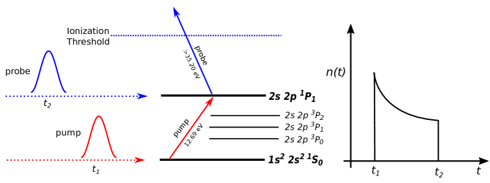
Figure 1: Scheme of a pump-probe experiment for atomic lifetime measurements of the $1s^{2}2s2p$ ${}^{1}P_{1}$ state in Be-like carbon. At time $t_{1}$ the XUV-pump pulse excites the $1s^{2}2s^{2}$ ${}^{1}S_{0}$ ground state of the Be-like carbon sample to the $1s^{2}2s2p$ ${}^{1}P_{1}$ excited state. The population $n(t)$ of the excited state ${}^{1}P_{1}$ decays then exponentially. A second and temporally delayed XUV-probe pulse probes the rest population of the excited state at time $t_{2}$ by ionizing Be-like carbon ion and maps out the exponential curve from which the decay rate is determined.

The excited state $1s^{2}2s2p$ ${}^{1}P_{1}$ decays to the $1s^{2}2s^{2}$ ${}^{1}S_{0}$ ground state through a strong spin allowed $E1$ transition. Therefore, the lifetime of the $1s^{2}2s2p$ ${}^{1}P_{1}$ state is defined by the line strength of this strong transition. During past years, various calculations have been reported for this line strength. Among these ab initio theories, particularly for the last three decades, are multiconfiguration Hartree-Fock (MCHF) Fischer (1994), multiconfiguration Dirac-Hartree-Fock (MCDHF) Ynnerman and Fischer (1995); Jönsson and Froese Fischer (1998); Wang et al. (2018), many-body perturbation theory (MBPT) Safronova et al. (1999), configuration-interaction (CI) method based on B-spline basis Chen et al. (2001) and configuration-interaction and many-body perturbation theory (CI+MBPT) Savukov (2004). As a result, the most accurate theoretical calculations Jönsson and Froese Fischer (1998); Chen et al. (2001) report an accuracy of the order $5\times 10^{-4}$. In view that the expected experimental accuracy is much better, there is a need for further improvements in the theoretical calculations.

Here, we present a detailed calculation of the line strength of the $1s^{2}2s2p$ ${}^{1}P_{1}\,-\ 1s^{2}2s^{2}$ ${}^{1}S_{0}$ transition in Be-like carbon on account of high precision experiment. We develop various electron correlation models and use orthogonal and nonorthogonal sets of orbitals for the initial and final states in these correlation models. It is found, that the accuracy assessment based on an agreement between the gauges might significantly lead to underestimate the uncertainty. For this reason, we estimate the uncertainty from the differences between the results obtained within all the correlation models developed. In addition, the finite nuclear mass effect on the line strength is evaluated and its gauge invariance is demonstrated after taking into account the recoil correction to the transition operator. As a result, the calculated line strength amounts to $2.43926(37)$ with the relative accuracy $1.5\times 10^{-4}$.

The following parts of the paper are structured as follows. In Sec. II, we present the underlying theory for the calculation of the transition energy and line strength. Details of the correlation models and results obtained are explained in Sec. III. In Sec. IV, we present theoretical methods for the finite nuclear mass effect. In the final section, we compare the obtained results with other theories and experiments and present the conclusion.

The atomic units $(\hbar=1,\,e=1,\,m_{e}=1)$ are used throughout the paper unless stated otherwise.

II theoretical methods

To effectively evaluate the electron-electron correlation effects, we apply systematically enlarged many-electron wave functions by using the general purpose relativistic atomic structure package Grasp2K Jönsson et al. (2013). This package implements the multiconfiguration Dirac-Hartree-Fock (MCDHF) method in $jj$-coupling Grant (2007); Fischer et al. (2016). In this method, the wave function $\Psi$ of a state labelled $\Gamma$, total angular momentum quantum number $J$ and parity $\pi$ is referred to as an atomic state function (ASF) which is represented as $\Psi(\Gamma;\pi J)$. It is an approximate eigenfunction of the Dirac-Coulomb Hamiltonian given by

$$\hat{H}_{\rm DC}=\sum_{i=1}^{N}\bigg{[}c\bm{\alpha}_{i}\cdot\bm{p}_{i}+(\beta_{i}-1)c^{2}-V(r_{i})\bigg{]}+\sum_{i<j}^{N}\frac{1}{r_{ij}}\,,$$ (1)

where $c$ is the speed of light, $\bm{\alpha}$ and $\beta$ are (4$\times$4) Dirac-matrices, $V(r_{i})$ is the potential of a two parameter Fermi nuclear charge distribution and $r_{ij}$ is the distance between electrons $i$ and $j$.

The ASF $\Psi(\Gamma;\pi J)$ is expanded in the basis of configuration state functions (CSFs) of the same symmetry:

$$\Psi{(\Gamma;\pi J)}=\displaystyle\sum_{j=1}^{n_{c}}c_{j}\Phi(\gamma_{j};\pi J),$$ (2)

where $n_{c}$ is the number of CSFs, $c_{j}$ are the mixing coefficients and $\gamma_{j}$ denotes the orbital occupancy and angular coupling scheme of the $j$-th CSF. The CSFs $\Phi(\gamma_{j};\pi J)$ are a linear combination of Slater determinants of one electron Dirac orbitals,

$$\phi_{n\kappa,m}(\bm{r})=\frac{1}{r}\begin{pmatrix}P_{n\kappa}\left(r\right)\chi_{\kappa}^{m}(\theta,\varphi)\\ iQ_{n\kappa}\left(r\right)\chi_{-\kappa}^{m}(\theta,\varphi)\end{pmatrix}.$$ (3)

Here, $\kappa$ is the relativistic angular momentum quantum number, $P_{n\kappa}\left(r\right)$ and $Q_{n\kappa}\left(r\right)$ are the large and small radial components of the one electron wave functions represented on a logarithmic grid, and $\chi_{\kappa}^{m}$ is the spinor spherical harmonic. The radial part of the Dirac orbitals and the expansion coefficients $c_{j}$ are optimized to self consistency from a set of equations which result from applying the variational principle in Dirac-Coulomb approximation Dyall et al. (1989). Here we have a choice of simultaneous or separate optimization of the orbitals for the desired ASFs. In the optimal level (OL) scheme a variational functional is constructed to minimize the energy for only one ASF, whereas in the extended optimal level (EOL) scheme the calculations can be extended to include several ASFs. In the latter case, the energy functional contains weights for the levels under consideration.

The line strength of the transition is defined as a square of the reduced nondiagonal matrix element of the electromagnetic operator:

$$S=\left|\left\langle\Psi(\Gamma;\pi J)||\boldsymbol{T}||\Psi(\Gamma^{\prime};\pi^{\prime}J^{\prime})\right\rangle\right|^{2}\,,$$ (4)

which after the optimization of the wave functions for the states $\Psi(\Gamma;\pi J)$ and $\Psi(\Gamma^{\prime};\pi^{\prime}J^{\prime})$ is calculated as

$$S=\Bigl{|}\sum_{j,k}c_{j}c^{\prime}_{k}\left\langle\Phi(\gamma;\pi J)||\boldsymbol{T}||\Phi(\gamma^{\prime};\pi^{\prime}J^{\prime})\right\rangle\Bigr{|}^{2}\,.$$ (5)

Here, $\boldsymbol{T}$ is $E1$ transition operator Grant (2007)

$$T^{l}_{M} = \frac{\sqrt{2\pi}c}{\omega}\sum_{i}^{N}\Bigl{[}-\sqrt{6}j_{1}(\omega r_{i}/c)Y_{1M}(\bm{n}_{i})$$ (6)

$$+ 3j_{2}(\omega r_{i}/c)c\bm{\alpha}_{i}\cdot\bm{Y}^{2}_{1M}(\bm{n}_{i})\Bigr{]}$$

in the length gauge and

$$T^{v}_{M} = \frac{\sqrt{2\pi}c}{\omega}\sum_{i}^{N}\Bigl{[}-\sqrt{2}j_{0}(\omega r_{i}/c)c\bm{\alpha}_{i}\cdot\bm{Y}^{0}_{1M}(\bm{n}_{i})$$ (7)

$$+ j_{2}(\omega r_{i}/c)c\bm{\alpha}_{i}\cdot\bm{Y}^{2}_{1M}(\bm{n}_{i})\Bigr{]}$$

in the velocity gauge. Here, $\omega$ is the transition energy, $Y_{JM}$ are the spherical harmonics, $\bm{Y}^{L}_{JM}$ are the spherical vectors, and $j_{J}(\omega r/c)$ is the spherical Bessel function. The operators (6) and (7) are used for the present calculations of the line strengths in length and velocity gauges. However, in order to investigate the dependence of the line strength on the transition energy we expand the Bessel functions $j_{J}(\omega r/c)\approx(\omega r/c)^{J}/(2J+1)!!$, the so-called long-wavelength approximation $\omega/c\ll 1$, and retain only the leading term in the power series expansion. In such a way the line strength takes a form:

$$S^{l}\approx\left|\left\langle\Psi(\Gamma;\pi J)||\sum_{i}^{N}\bm{r}_{i}||\Psi(\Gamma^{\prime};\pi^{\prime}J^{\prime})\right\rangle\right|^{2}$$ (8)

in the length gauge and

$$S^{v}\approx\frac{c^{4}}{\omega^{2}}\left|\left\langle\Psi(\Gamma;\pi J)||\sum_{i}^{N}\bm{\alpha}_{i}||\Psi(\Gamma^{\prime};\pi^{\prime}J^{\prime})\right\rangle\right|^{2}$$ (9)

in the velocity gauge. From the expressions  (8) and (9) one can see, that the leading term of the line strength in the length form is insensitive to the transition energy whereas in the velocity form it is proportional to $\omega^{-2}$. Based on these observations one can introduce the semi-empirical correction to the line strength in the velocity gauge by adjusting the transition energy to a more accurate, e.g., experimental, value, i.e., $\Delta S^{v}=(\omega^{2}-\omega_{\rm exp}^{2})/\omega_{\rm exp}^{2}\,S^{v}$. Such a correction allows to take partially into account the missing correlation contributions. The line strength in the velocity gauge adjusted in this way $S^{v}_{({\rm exp})}$ is typically much closer to the value in the length gauge $S^{l}$. Generally, the gauge invariance should be restored when all correlation effects are taken into account, both for the transition matrix element and transition energy, which was explicitly demonstrated in the framework of the relativistic many-body perturbation theory Savukov and Johnson (2000) and QED formalism Indelicato et al. (2004). In view of this, the excellent agreement between the gauges after adjustment suggests that the remaining unaccounted correlation effects to the transition amplitude are rather small. As a result, the difference between the line strengths calculated in the length gauge and adjusted value in the velocity gauge is employed for the theoretical error estimation Fischer (2009, 2010). However, it is still possible that the remaining unaccounted correlation effects not only reduce the discrepancy between the gauges but also shift both values by an amount, which is much larger than the difference between the gauges after adjustment.

III correlation models

In a view of an absence of strong criteria for the uncertainty estimation of the calculated line strength, we performed the MCDHF calculations for different correlations models. Among those models, we choose only four models based on the accuracy criterion for the transition energy as it is compared with the experimental energy. These four models were based on separate and simultaneous (orthogonal and nonorthogonal) set of orbitals for the ground and excited states. In each model, the correlations were incorporated by systematically extending the calculations in a series of steps. As a first step, the calculations were performed for the lowest order of approximation where the orbitals belonging to so-called reference configurations were spectroscopically optimized, i.e., orbitals were required to have a node structure similar to the corresponding hydrogenic orbitals Fischer et al. (2016). Here the reference configurations for the first three models were {$1s^{2}2s^{2}$, $1s^{2}2p^{2}$} for the ${}^{1}S_{0}$ ground state and {$1s^{2}2s2p$} for the ${}^{1}P_{1}$ excited state. For the fourth model, the reference configurations were increased and we explain its details later in this section. In the latter steps, the calculations were extended by expanding the basis set of CSFs using the active set approach. In this approach, the correlations are incorporated by virtually exciting the electrons from spectroscopic reference configurations to a set of orbitals called the active set of orbitals. We increased the active set by adding a layer of correlation orbitals but optimized only the outermost layer and kept the remaining orbitals fixed from the previous step of calculations.

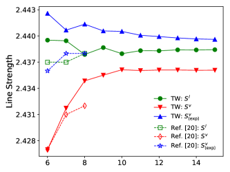
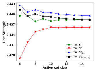
Figure 2: Comparison of the line strengths evaluated according to the Model 1 (TW) as a function of active set size of the orbitals with the results of Ref. Jönsson and Froese Fischer (1998). The green circles, red down triangles, and blue upper triangles display the present calculations in the length gauge $S^{l}$ as well as in velocity gauges before $S^{v}$ and after adjustment $S^{v}_{(\rm exp)}$ to the experimental transition energy $\omega_{\rm exp}$, respectively. The green hollow squares, red hollow diamonds, and blue hollow stars are corresponding values taken from Ref. Jönsson and Froese Fischer (1998).

We now explain how valence-valence (VV), core-valence (CV) and core-core (CC) correlations were incorporated. We started to expand the basis set by adding the CSFs that are generated from the configurations $1s^{2}nln^{\prime}l^{\prime}$ which result from single and double (SD) excitations from outer shells of the reference configuration. These CSFs account VV correlations and the calculations are named as VV calculations. To each layer of VV correlation calculations, we then added CSFs of the configurations $1s2snln^{\prime}l^{\prime}+1s2pnln^{\prime}l^{\prime}$ which arise from the single excitation from the $1s^{2}$ core with or without another excitation from the valence shells. These added CSFs account for the CV correlations and the calculations are called VV+CV. Now with each layer of VV+CV correlation calculations, the correlations of two-electron excitations from the $1s^{2}$ core were included to account for the CC correlations. These additional CSFs arise from the configurations $2s^{2}nln^{\prime}l^{\prime}+2p^{2}nln^{\prime}l^{\prime}$ for the ${}^{1}S_{0}$ state and $2s2pnln^{\prime}l^{\prime}$ for the ${}^{1}P_{1}$ state. These correlation calculations are named as VV+CV+CC calculations. In all VV, VV+CV and VV+CV+CC calculations, the active set of orbitals was spanned by the orbitals with principal quantum number $n,n^{\prime}\leq 15$ and with azimuthal quantum number $l,l^{\prime}\leq 7$. Finally, the basis set of CSFs was expanded by appending CSFs with configurations arising from single, double, triple and quadruple (SDTQ) excitations from the reference configurations. In the SDTQ excitations the number of CSFs increased very rapidly with the increasing number of orbitals in the active set which challenges the numerical stability and available hardware resources. So the SDTQ excitations were limited only with $n,n^{\prime}\leq 5$ and $l,l^{\prime}\leq 4$. These calculation were then extended with SD excitations with remaining layer of correlation orbitals with $n,n^{\prime}\leq 15$ and $l,l^{\prime}\leq 7$. We name this final set of calculations as VV+CV+CC:SDTQ.

III.1 Model 1

In this model the VV and VV+CV calculations were performed by utilizing the OL scheme for the ground and excited state, i.e., for both states orbitals are separately optimized, whereas for the VV+CV+CC as well as VV+CV+CC:SDTQ calculations the spectroscopic orbitals and the correlation orbitals with $n=3$ were simultaneously optimized using the EOL scheme. Then the calculations after $n=3$ were extended with a separate set of correlation orbitals (the OL scheme). This model accounts for the correlations in a similar manner as those presented by Jönsson and Froese Fischer Jönsson and Froese Fischer (1998). The only difference is that Jönsson and Froese Fischer performed VV+CV+CC:SDTQ calculations with SDTQ excitation until $n=3$ only and extended their calculations from $n>3$ with VV+CV type of correlations only.

Table 1: Transition energies $\omega$ (cm^-1) and line strengths $S$ (a.u.) for the $1s^{2}2s2p$ ${}^{1}P_{1}\,-\ 1s^{2}2s^{2}$ ${}^{1}S_{0}$ transition in Be-like carbon as functions of the active set calculated within Model 1. The line strengths in the length gauge ($S^{l}$) are compared with those in the velocity gauge ab initially calculated ($S^{v}$) and after adjustment to the experimental energy $\omega_{\rm exp}$ ($S^{v}_{({\rm exp})}$) and to the experimental-Dirac-Coulomb energy $\omega_{\rm exp-DC}$ ($S^{v}_{({\rm exp-DC)}}$). The experimental transition energy is taken from Ref. Kramida et al. (2018), while the experimental-Dirac-Coulomb energy is evaluated by subtracting the Breit, recoil, and QED corrections from the experimental transition energy.

Active set	$\omega$	$S^{l}$	$S^{v}$	$S^{v}_{({\rm exp})}$	$S^{v}_{({\rm exp-DC})}$
DHF	112 958	2.34092	1.65645	2.01753	2.01651
$3s3p3d$	104 094	2.51432	2.36757	2.44884	2.44759
$4s4p4d4f$	103 116	2.45884	2.38001	2.41568	2.41446
$5s5p5d5f5g$	102 804	2.44978	2.40435	2.42565	2.42442
$6s6p6d6f6g6h$	102 680	2.43952	2.42699	2.44259	2.44135
$7s7p7d7f7g7h7i$	102 540	2.43945	2.43173	2.44067	2.43943
$8s8p8d8f8g8h8i8k$	102 488	2.43788	2.43486	2.44135	2.44011
$9s9p9d9f9g9h9i9k$	102 459	2.43867	2.43551	2.44058	2.43934
$10s10p10d10f10g10h10i10k$	102 444	2.43797	2.43613	2.44052	2.43928
$11s11p11d11f11g11h11i10k$	102 437	2.43832	2.43604	2.44008	2.43884
$12s12p12d12f12g12h12i10k$	102 432	2.43830	2.43610	2.43993	2.43869
$13s13p13d13f13g13h13i10k$	102 429	2.43841	2.43610	2.43977	2.43853
$14s14p14d14f14g14h14i10k$	102 427	2.43840	2.43607	2.43966	2.43842
$15s15p15d15f15g15h15i10k$	102 426	2.43843	2.43608	2.43961	2.43837
Due to other models	-15
Breit	-3
Recoil	-13
QED	-10
Total	102 385
Exp	102 352
Exp-DC	102 378

In Fig. 2 (upper plot) we compare the present calculations of Model 1 with Jönsson and Froese Fischer results Jönsson and Froese Fischer (1998). The line strength in length and velocity form is plotted against increasing $n$ of the active set size defining the wave function expansion in respective calculations. It is clearly evident that their two gauges agree perfectly at $n=8$ once the experimental energy adjustment was applied. Explicitly, the line strength calculated in Ref. Jönsson and Froese Fischer (1998) amounts to 2.4376 in the length gauge and 2.4366 in the velocity gauge after adjustment, which leads to a tabulated final value 2.4376(13). Despite we can not explicitly reproduce these calculations, our evaluations show the similar effect at $n=7$ active set layer, where the results obtained in the length and velocity (adjusted) gauges approach each other. However, when the active set size is further extended, one can clearly see that after $n=7$ layer the results first drift apart and then, again, approach each other but at some different position. These observations lead us to the following conclusions. First, the agreement between gauges might be of an accidental character and, therefore, second, the difference between results in the length and velocity (adjusted) gauges should be very carefully used as a criterion for the error estimation.

Let us mention here another important observation. From the basic theory Savukov and Johnson (2000); Indelicato et al. (2004), it is clear that the adjustment should be made to the transition energy which corresponds to the difference of the eigenvalues of the Dirac-Coulomb Hamiltonian in Eq. (1). Therefore, we calculate a so-called experimental-Dirac-Coulomb transition energy $\omega_{\rm exp-DC}$ as a difference of the experimental value $\omega_{\rm exp}$ and the contributions beyond the Dirac-Coulomb approximation, i.e., the Breit interaction, recoil, and QED corrections. The $\omega_{\rm exp-DC}$ energy is, thus, experimentally deduced fully correlated Dirac-Coulomb transition energy. We compare in Table 1 as well as in Fig. 2 (lower plot) the line strengths in the length gauge ($S^{l}$) and in the velocity gauge (ab initio) ($S^{v}$) with the adjusted to $\omega_{\rm exp}$ ($S^{v}_{({\rm exp})}$) and to $\omega_{\rm exp-DC}$ ($S^{v}_{({\rm exp-DC})}$) values. As one can see from this comparison the values adjusted to the experimental-Dirac-Coulomb energy are much close to the results in the length gauge. In particular, for $n=15$ layer the relative difference between the gauges amounts to $2\times 10^{-5}$. However, as we mention at the end of Sec. II the agreement between the gauges cannot be uniquely used for the accuracy assessment. For this reason, in the next subsections, we investigate also other correlation models.

III.2 Model 2

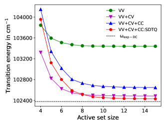
Figure 3: Extent of different correlations effects to the transition energy with respect to the increasing $n$ of the active set size defining the wave function expansion for the Model 2 calculations. The green circles represent VV correlations, magenta down triangles represent VV+CV, blue upper triangles represent VV+CV+CC, red-pentagons represent VV+CV+CC:SDTQ correlations. Please see the text for the details of different type of the correlations.

Within this model, both the spectroscopic and the correlations orbitals were separately optimized using the OL scheme for all type of correlations. Hence generated orbitals for both states were not quite orthogonal with each other, which makes the implementation of standard Racah algebra difficult for the calculation of transition amplitude. To deal with this complication, a transformation to a biorthonormal basis was applied together with the counter transformation of the expansion coefficients $c_{j}$ and $c^{\prime}_{k}$ Olsen et al. (1995).

The calculations within this model show the importance of a common set of orbitals for the core correlations in the framework of MCDHF approach. For the CC effects, it is commonly accepted that these are more balanced if a common orbital basis is used for describing both the states involved in the transition and hence resulting transition energies are more accurate, for details please see the Ref. Bieroń et al. (2018); Filippin et al. (2016). This is also obvious from Fig. 3 where the evaluation of different correlations effects to the transition energy is shown with respect to the increasing $n$ of the active set size defining the wave function expansion for the Model 2 calculations. Here the blue upper triangles representing VV+CV+CC correlation results are worse than the magenta down triangles representing VV+CV correlations. However, it is obvious from the red-pentagons representing VV+CV+CC:SDTQ in Fig. 3 that we get the best agreement of the transition energy with the experiment when the TQ excitations are included with SD excitations in the CC correlations. The difference of the final values of the energy of VV+CV+CC:SDTQ calculations with Model 1 and Model 2 is only 0.004%, whereas the length form of the line strength from both models varies only by 0.01%. The fact that TQ contributions are very important is also noticed from the results of Chen, Cheng and Johnson Chen et al. (2001) who have also used TQ excitations in building a common set of orbitals in their RCI calculations based on B-spline basis.

III.3 Model 3

Within this model, both the spectroscopic orbitals and correlations orbitals were simultaneously optimized for the ground and excited states using the EOL scheme for all type of correlations. The so obtained orbitals for both states were orthogonal to each other. As it has been highlighted by Chen, Cheng and Johnson Chen et al. (2001) and Savukov Savukov (2004) that small orbital overlap corrections due to nondiagonal set of orbitals for the initial and final state should not be ignored. Our correlation Model 3 helped to address this issue.

III.4 Model MR

In this model, the set of spectroscopic reference configurations were expanded to account the missing correlations due to limited SDTQ excitations. We name it as multi-reference (MR) model. The configurations in MR are expanded in such a way that the CSFs for the MR set had the largest expansion coefficients in the wave functions that were generated by VV+CV+CC:SDTQ calculations of Model 3. For the ${}^{1}S_{0}$ ground state the resulting MR set was {$1s^{2}2s^{2},1s^{2}2p^{2},1s^{2}3p^{2},2s^{2}3s^{2},2s^{2}3p^{2},1s^{2}3d^{2}$} and for the ${}^{1}P_{1}$ excited state the resulting MR set was {$1s^{2}2s2p,1s^{2}2p3d,2s2p3s^{2},2s2p3p^{2}$}. All the orbitals occupied in MR set were spectroscopically treated in the lowest order of approximation. Then the correlation orbitals were treated in the same way as those of Model 3 using the EOL scheme.

III.5 Models: summary

Our approach with either a common or two separate set of orbitals for the ground and excited states combines the strengths and weaknesses of the previous calculations which provide the uncertainty of the order of $10^{-3}$ Jönsson and Froese Fischer (1998); Chen et al. (2001); Savukov (2004). The orbitals in the common set for both states are orthogonal to each other and there is no orbital overlap for the evaluation of the transition amplitude. At the same time, our procedure of two different sets of orbitals for each state has the advantage that the electron relaxation effects are automatically included to a large extent.

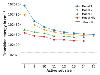
Figure 4: Convergence of transition energy with respect to the increasing $n$ of the active set size defining the wave function expansion for the VV+CV+CC:SDTQ calculations of different correlation models. Please see the text for the details of the VV+CV+CC:SDTQ calculations.

In all our correlation models the overall convergence trends and behavior of the inner and outer electron correlations are consistent with each other. In Fig. 4 we present the convergence of the transition energy with respect to the increasing $n$ of the active set size defining the wave function expansion for the VV+CV+CC:SDTQ calculations from all the correlation models under present study. For the Model 3 and MR we could not get the converged orbitals for $n=15$. The first three models vary just with a difference of maximum of 6 cm^-1. But for Model MR we get 15 cm^-1 better results and this is obviously due to the inclusion of higher-order correlations in this model.

In Fig. 5 we present the line strength for the VV+CV+CC:SDTQ correlations calculated within Model 2, 3, and MR in a similar way as explained in Sec. III.1 and Fig. 2 (lower plot). From these plots, one can clearly see that in all models the line strength in the velocity adjusted to the experimental-Dirac-Coulomb energy agrees with the length gauge result much better than the adjusted to the pure experimental energy. This also confirms our expectations originated from the basic principles as stated at the end of Sec. III.1. In order to get the final (Dirac-Coulomb) line strength value the results of the length gauge and adjusted to the experimental-Dirac-Coulomb energy velocity gauge obtained at the maximum active set size are analysed. The employed data from all the correlation models are summarized in Table 2 and Fig. 6. As one can see from these data, despite the extraordinary agreement between gauges, e.g., in Model 1, one can not use it for the uncertainty estimation. The reason for this has been explained at the end of Sec. II and confirmed now by the calculations in other models, which predict quite larger spread of the results than given by the difference of the gauges. We take an average of these scatter of the line strength data to predict the final value of the line strength and take one standard deviation of these scatter of the line strength data to predict the uncertainty in the results. As a result, present line strength accounting only the correlations is 2.43851(37). This is represented as a black solid line in Fig. 6, whereas in this figure the uncertainty is shown as a gray shaded region. We find rather conservative to assess the uncertainty as one standard deviation of the scattered data. Such kind of an error estimation is further supported by the fact that it covers all the values obtained in the length gauge, which is known to be more reliable.

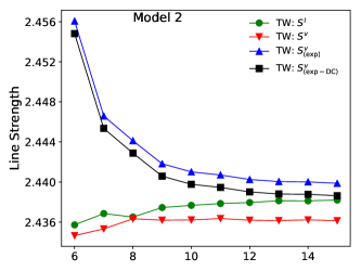
(a)

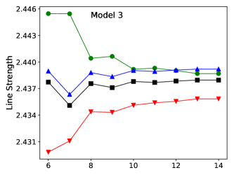
(b)

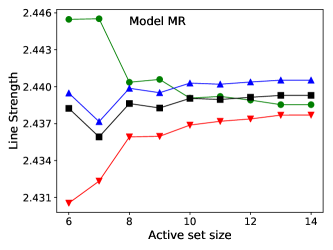
(c)

Figure 5: Line strength for the for the VV+CV+CC:SDTQ calculations from the Model 2, Model 3 and Model MR plotted similarly as that of Fig. 2. In each sub-figure, the green circles are the line strength $S^{l}$ in length form, red down triangles are ab initio $S^{v}$ velocity from, blue upper triangles are $S^{v}_{(\rm exp)}$ velocity form adjusted the experimental transition energy $\omega_{\rm exp}$ and black squares are $S^{v}_{({\rm exp-DC})}$ velocity from adjusted the experimental-Dirac-Coulomb transition energy $\omega_{\rm exp-DC}$ (see text).

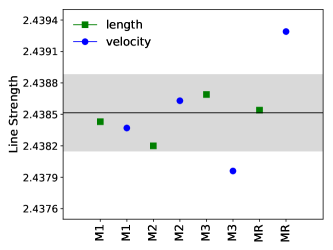
Figure 6: Line strength of the $1s^{2}2s2p$ ${}^{1}P_{1}\,-\ 1s^{2}2s^{2}$ ${}^{1}S_{0}$ transition in Be-like carbon plotted against the present Models. Green squares correspond to the length-form values and blue circles to the velocity-form values. The black solid line is the average of the both length and velocity forms. The gray shaded region is one standard deviation with respect to the black line.

Table 2: $\omega$ is the Dirac-Coulomb transition energy (cm^-1). $S^{l}$ and $S^{v}_{({\rm exp-DC})}$ are the Dirac-Coulomb line strengths in the length gauge and in the velocity gauge adjusted to $\omega_{\rm exp-DC}$ energy (see text), in a.u.

Label	$\omega$	$S^{l}$	$S^{v}_{({\rm exp-DC})}$
Model 1	102426	2.43843	2.43837
Model 2	102430	2.43820	2.43863
Model 3	102423	2.43869	2.43796
Model MR	102411	2.43854	2.43929
Final		2.43851(37)

IV nuclear recoil correction

Once the line strength is calculated, including all the major correlation contributions, the finite nuclear mass (nuclear recoil) contribution was added as a correction given as

$$\Delta S_{\mathrm{rec}}=\Delta S_{\mathrm{rec,en}}+\Delta S_{\mathrm{rec,wf}}+\Delta S_{\mathrm{rec,op}},$$ (10)

where the first two terms on the right side in Eq. (10) are the corrections to the line strength due to nuclear-recoil contributions to the energy and wave functions. These corrections were calculated using the relativistic configuration interaction (RCI) program of Grasp2K Jönsson et al. (2013). Here the lowest order nuclear motional corrections, namely the normal mass shift (NMS) term based on Dirac kinetic energy operator

$$\hat{H}_{\mathrm{NMS}}=\frac{1}{M}\sum_{i=1}^{N}\Bigl{[}c\boldsymbol{\alpha}_{i}\cdot\boldsymbol{p}_{i}+(\beta_{i}-1)c^{2}\Bigr{]},$$

where the $M$ is the nuclear mass, and mass polarization term named as the specific mass shift (SMS)

$$\hat{H}_{\mathrm{SMS}}=\frac{1}{M}\sum_{i<j=1}^{N}\bm{p}_{i}\cdot\bm{p}_{j},$$

were added to the Dirac-Coulomb Hamiltonian, Eq. (1). The additional relativistic corrections to the recoil operators are of the order $(Z\alpha)^{2}$ Karshenboim (1997). For $Z=6$, these corrections are in the order of $10^{-6}$, which is far below than present level of uncertainty. However, the relativistic corrections must be taken into considerations for the future studies of higher $Z$.

It is also important, however, to take into account the recoil correction to the transition operator, i.e., the third term in Eq. (10). Previously, it was considered in Refs. Fried and Martin (1963); Yan and Drake (1995); Karshenboim (1997); Yan et al. (1998) for the $E1$ transitions and in Ref. Volotka et al. (2008) for the $M1$-decay. Starting from the nonrelativistic Hamiltonian for $N$ electrons and the nucleus, we obtain the following recoil corrections to the $E1$ transition operator:

$$\Delta\boldsymbol{T}^{l}_{\rm rec}=-\frac{Z-N}{M}\sum_{i=1}^{N}\bm{r}_{i}$$ (11)

in the length gauge and

$$\Delta\boldsymbol{T}^{v}_{\rm rec}=-\frac{Z}{M}\frac{1}{\omega}\sum_{i=1}^{N}\bm{p}_{i}$$ (12)

in the velocity gauge. From these expressions one can easily come to the corresponding corrections to the line strength

$$\Delta S^{l}_{\rm rec,op} = 2{\rm Re}\left\{\langle\Psi(\Gamma;\pi J)||\boldsymbol{T}^{l}||\Psi(\Gamma^{\prime};\pi^{\prime}J^{\prime})\rangle\right.$$ (13)

$$\times \left.\langle\Psi(\Gamma;\pi J)||\Delta\boldsymbol{T}^{l}_{\rm rec}||\Psi(\Gamma^{\prime};\pi^{\prime}J^{\prime})\rangle\right\}$$

$$\approx 2\frac{Z-N}{M}S^{l}$$

and

$$\Delta S^{v}_{\rm rec,op} = 2{\rm Re}\left\{\langle\Psi(\Gamma;\pi J)||\boldsymbol{T}^{v}||\Psi(\Gamma^{\prime};\pi^{\prime}J^{\prime})\rangle\right.$$ (14)

$$\times \left.\langle\Psi(\Gamma;\pi J)||\Delta\boldsymbol{T}^{v}_{\rm rec}||\Psi(\Gamma^{\prime};\pi^{\prime}J^{\prime})\rangle\right\}$$

$$\approx 2\frac{Z}{M}S^{v}\,.$$

Table 3: The recoil corrections to the line strength originated from the energy and wave functions change, $\Delta S_{\rm rec,en+wf}$, as well as due to the transition operator $\Delta S_{\rm rec,op}$ calculated in the length and velocity gauges. The total gauge invariant recoil correction is presented in the last line. The values are in a.u.

Rec. correction	length	velocity
$\Delta S_{\rm rec,en+wf}$	0.00000	$-$0.00089
$\Delta S_{\rm rec,op}$	0.00045	0.00134
Total	0.00045	0.00045

In Table 3 different recoil contributions due to the energy, wave functions, and operator are presented in the length and velocity gauges. Only with the term due to the change of the operator included the total recoil correction is gauge invariant. In view of this, we would recommend to introduce this contribution also to the next GRASP update.

V discussion and conclusion

Table 4: Comparisons between different calculations and experiments for the line strength of the $1s^{2}2s2p$ ${}^{1}P_{1}\,-\ 1s^{2}2s^{2}$ ${}^{1}S_{0}$ transition and the lifetime of the $1s^{2}2s2p$ ${}^{1}P_{1}$ excited state in Be-like carbon.

$S$ [a.u.]	$\tau$ [ns]	Ref.
Theories
2.434(6)	0.5673(13)	Fischer (1994)
2.435(6)	0.5671(13)	Ynnerman and Fischer (1995)
2.4376(13)	0.56650(30)	Jönsson and Froese Fischer (1998)
2.057	0.6713	Safronova et al. (1999)
2.4377(10)	0.56648(23)	Chen et al. (2001)
2.4390(24)	0.56618(55)	Savukov (2004)
2.436	0.5669	Wang et al. (2018)
2.43926(40)	0.56612(9)	Present work
Experiments
2.09(1)	0.66(3)	Heroux (1969)
2.16(2)	0.64(6)	Poulizac and Buchet (1971)
2.09(2)	0.66(7)	Buchet-Poulizac and Buchet (1973)
2.76(1)	0.50(3)	Chang (1977)
2.42(1)	0.57(2)	Reistad et al. (1986)
2.426(45)	0.569(10)	Reistad and Martinson (1986)

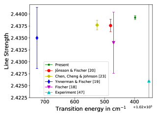
Figure 7: A comparison of the present line strength of the $1s^{2}2s2p$ ${}^{1}P_{1}\,-\ 1s^{2}2s^{2}$ ${}^{1}S_{0}$ transition in Be-like carbon with other theories and experiment.

With the discussion above, we can obtain the final value of the line strength. In order to do so, we add to the Dirac-Coulomb value 2.43851(37) from Sec. III the recoil correction $\Delta S_{\rm rec}=0.00045$ calculated in the previous section. In addition, we have to consider also other effects, such as the Breit interaction as well as QED. The Breit contribution has been calculated as follows. The frequency-independent Breit Hamiltonian has been added to the Dirac-Coulomb Hamiltonian given by Eq. (1). Then the RCI calculations have been performed within the correlation Model 1. Comparing further the obtained results with the corresponding Dirac-Coulomb values we get for the Breit contribution $\Delta S_{\rm Breit}$ $0.00030$ and $-0.00001$ in the length and velocity gauge, respectively. Based on an analysis of the Breit contribution in the intercombination transition $2s2p$ ${}^{3}P_{1}\,-\ 2s^{2}$ ${}^{1}S_{0}$ in Be-like carbon Ref. Chen et al. (2001) and on arguments presented in Refs. Johnson et al. (1995); Derevianko et al. (1998), we attribute this difference to the negative-energy corrections. That means that the gauge invariance of the Breit contribution should be restored when the negative-energy states will be accurately taken into account. On the other hand, it was demonstrated Johnson et al. (1995); Derevianko et al. (1998), that the negative-continuum affects dominantly only the result in the velocity gauge, while the result of the length gauge remains stable. In view of this, we add the Breit correction calculated in the length gauge and with the 50% uncertainty, $\Delta S_{\rm Breit}=0.00030(15)$, to our final value. The remaining QED correction is estimated as $\alpha(\alpha Z)^{2}{\rm ln}(\alpha Z)^{-1}$ Ivanov and Karshenboim (1996); Sapirstein et al. (2004) to be $4\times 10^{-5}$, which is much smaller than our uncertainty. As a result, our final value for the line strength reads 2.43926(40), where the uncertainty is coming from the correlations and Breit contribution.

Once the line strength is calculated, it is straightforward to get the weighted oscillator strength $gf$:

$$gf=\frac{2}{3}\omega S,$$ (15)

and the lifetime of the $1s^{2}2s2p$ ${}^{1}P_{1}$ excited state:

$$\tau=\frac{3g}{4}\frac{c^{3}}{\omega^{3}S}\,,$$ (16)

where $g$ is the weight of the upper state. Here the conversion to the lifetime form the line strength and vice versa is performed by using the experimental energy, $\omega=102352.04$ cm^-1 Kramida et al. (2018). We note that the present uncertainty in the lifetime is only due to calculated line strength, since the uncertainty of the transition energy is expected to be much better than 1 cm^-1 and this is far below the uncertainty of the line strength.

Fig. 7 and Table 4 compare the present results of calculated line strength and lifetime with other theories and experiments. Note that in the respective papers the values of oscillator strength is provided. We have converted the oscillator strength to the line strength using the energies mentioned in the respective papers. In Fig. 7, the experimental line strength reported in Ref. Reistad and Martinson (1986) is plotted as a function of the experimental energy taken from the NIST database Kramida et al. (2018). It is clear from Fig. 7 that our calculated energy is the closest to the experimental one. The present line strength or lifetime agrees very well with the CI+MBPT calculation of Savukov Savukov (2004) and is in a fair agreement with the large-scale MCDF calculation of Jönsson and Froese Fischer Jönsson and Froese Fischer (1998) and the CI result of Chen, Cheng and Johnson Chen et al. (2001).

It is obvious from the Table 4 that all the theoretical lifetimes except of Ref. Safronova et al. (1999) are inside the error bar of the best available experimental lifetime of 0.569(10) ns Reistad and Martinson (1986). However, the uncertainty of this measurement is still too large to distinguish between different theories. Therefore, we hope that the proposed experiment in Ref. Rothhardt et al. (2019) will provide a new benchmark for testing the theories in the case of Be-like carbon.

In conclusion, we have presented high precision atomic calculations of the line strength of the $1s^{2}2s2p$ ${}^{1}P_{1}\,-\ 1s^{2}2s^{2}$ ${}^{1}S_{0}$ spin allowed $E1$ transition in Be-like carbon. We have utilized the state-of-the-art multiconfiguration Dirac-Hartree-Fock method. In these systematically enlarged wave functions, we incorporated higher-order electron correlations, where the orbital relaxation and overlaps are taken into account by using separate and simultaneous sets of relativistic orbitals in the active set. This helped us to reliably estimate the uncertainty of the obtained line strength. Moreover, the finite nuclear mass correction to the line strength is calculated by correcting the energy, wave functions as well as the transition operator. The achieved relative uncertainty of the line strength amounts to $10^{-4}$, which represents a reliable theoretical benchmark of the $E1$ line strength in a view of upcoming high precision lifetime measurement of the $1s^{2}2s2p$ ${}^{1}P_{1}$ state of Be-like carbon.

Extensions of current studies to heavier Be-like ions allow us to improve the theoretical accuracy of transition rates. The given (numerical) uncertainty together with the high precision experiments will allow an alternative spectroscopic test than the energy alone and will provide further insight into the atomic structure of many-electron atoms and ions.

References

- Zhang and Ye (2016) X. Zhang and J. Ye, National Science Review 3, 189 (2016).
- López-Urrutia (2016) J. R. C. López-Urrutia, Journal of Physics: Conference Series 723, 012052 (2016).
- Kraft-Bermuth et al. (2018) S. Kraft-Bermuth, D. Hengstler, P. Egelhof, C. Enss, A. Fleischmann, M. Keller, and T. Stöhlker, Atoms 6, 040059 (2018).
- Volotka et al. (2013) A. V. Volotka, D. A. Glazov, G. Plunien, and V. M. Shabaev, Annalen der Physik 525, 636 (2013).
- Shabaev et al. (2018) V. M. Shabaev, A. I. Bondarev, D. A. Glazov, M. Y. Kaygorodov, Y. S. Kozhedub, I. A. Maltsev, A. V. Malyshev, R. V. Popov, I. I. Tupitsyn, and N. A. Zubova, Hyperfine Interactions 239, 60 (2018).
- Safronova et al. (2018) M. S. Safronova, D. Budker, D. DeMille, D. F. J. Kimball, A. Derevianko, and C. W. Clark, Rev. Mod. Phys. 90, 025008 (2018).
- Träbert (2014) E. Träbert, Atoms 2, 15 (2014).
- Träbert (2010) E. Träbert, Journal of Physics B: Atomic, Molecular and Optical Physics 43, 074034 (2010).
- Lapierre et al. (2005) A. Lapierre, U. D. Jentschura, J. R. Crespo López-Urrutia, J. Braun, G. Brenner, H. Bruhns, D. Fischer, A. J. González Martínez, Z. Harman, W. R. Johnson, C. H. Keitel, V. Mironov, C. J. Osborne, G. Sikler, R. Soria Orts, V. Shabaev, H. Tawara, I. I. Tupitsyn, J. Ullrich, and A. Volotka, Phys. Rev. Lett. 95, 183001 (2005).
- Brenner et al. (2007) G. Brenner, J. R. C. López-Urrutia, Z. Harman, P. H. Mokler, and J. Ullrich, Phys. Rev. A 75, 032504 (2007).
- Zewail (2000) A. H. Zewail, The Journal of Physical Chemistry A 104, 5660 (2000).
- Sell et al. (2011) J. F. Sell, B. M. Patterson, T. Ehrenreich, G. Brooke, J. Scoville, and R. J. Knize, Phys. Rev. A 84, 010501 (2011).
- Patterson et al. (2015) B. M. Patterson, J. F. Sell, T. Ehrenreich, M. A. Gearba, G. M. Brooke, J. Scoville, and R. J. Knize, Phys. Rev. A 91, 012506 (2015).
- Träbert (2014) E. Träbert, Applied Physics B 114, 167 (2014).
- Rothhardt et al. (2019) J. Rothhardt, M. Bilal, R. Beerwerth, A. V. Volotka, V. Hilbert, T. Stöhlker, S. Fritzsche, and J. Limpert, X-Ray Spectrometry (In Press 2019).
- Demmler et al. (2013) S. Demmler, J. Rothhardt, S. Hädrich, M. Krebs, A. Hage, J. Limpert, and A. Tünnermann, Opt. Lett. 38, 5051 (2013).
- Rothhardt et al. (2014) J. Rothhardt, S. Hädrich, S. Demmler, M. Krebs, S. Fritzsche, J. Limpert, and A. Tünnermann, Phys. Rev. Lett. 112, 233002 (2014).
- Fischer (1994) C. F. Fischer, Physica Scripta 49, 323 (1994).
- Ynnerman and Fischer (1995) A. Ynnerman and C. F. Fischer, Phys. Rev. A 51, 2020 (1995).
- Jönsson and Froese Fischer (1998) P. Jönsson and C. Froese Fischer, Phys. Rev. A 57, 4967 (1998).
- Wang et al. (2018) K. Wang, Z. B. Chen, C. Y. Zhang, R. Si, P. Jönsson, H. Hartman, M. F. Gu, C. Y. Chen, and J. Yan, Astrophys. J. Suppl. Ser. 234, 40 (2018).
- Safronova et al. (1999) U. I. Safronova, W. R. Johnson, M. S. Safronova, and A. Derevianko, Physica Scripta 59, 286 (1999).
- Chen et al. (2001) M. H. Chen, K. T. Cheng, and W. R. Johnson, Phys. Rev. A 64, 042507 (2001).
- Savukov (2004) I. M. Savukov, Phys. Rev. A 70, 042502 (2004).
- Jönsson et al. (2013) P. Jönsson, G. Gaigalas, J. Bieroń, C. F. Fischer, and I. Grant, Comput. Phys. Commun. 184, 2197 (2013).
- Grant (2007) I. P. Grant, Relativistic Quantum Theory of Atoms and Molecules: Theory and Computation (Springer, New York, 2007).
- Fischer et al. (2016) C. F. Fischer, M. Godefroid, T. Brage, P. Jönsson, and G. Gaigalas, Journal of Physics B: Atomic, Molecular and Optical Physics 49, 182004 (2016).
- Dyall et al. (1989) K. Dyall, I. Grant, C. Johnson, F. Parpia, and E. Plummer, Comput. Phys. Commun. 55, 425 (1989).
- Savukov and Johnson (2000) I. M. Savukov and W. R. Johnson, Phys. Rev. A 62, 052506 (2000).
- Indelicato et al. (2004) P. Indelicato, V. M. Shabaev, and A. V. Volotka, Phys. Rev. A 69, 062506 (2004).
- Fischer (2009) C. F. Fischer, Physica Scripta T134, 014019 (2009).
- Fischer (2010) C. F. Fischer, Journal of Physics B: Atomic, Molecular and Optical Physics 43, 074020 (2010).
- Kramida et al. (2018) A. Kramida, Yu. Ralchenko, J. Reader, and and NIST ASD Team, NIST Atomic Spectra Database (ver. 5.6.1), [Online]. Available: https://physics.nist.gov/asd [2019, February 18]. National Institute of Standards and Technology, Gaithersburg, MD. (2018).
- Olsen et al. (1995) J. Olsen, M. R. Godefroid, P. Jönsson, P. A. Malmqvist, and C. F. Fischer, Phys. Rev. E 52, 4499 (1995).
- Bieroń et al. (2018) J. Bieroń, L. Filippin, G. Gaigalas, M. Godefroid, P. Jönsson, and P. Pyykkö, Phys. Rev. A 97, 062505 (2018).
- Filippin et al. (2016) L. Filippin, R. Beerwerth, J. Ekman, S. Fritzsche, M. Godefroid, and P. Jönsson, Phys. Rev. A 94, 062508 (2016).
- Fried and Martin (1963) Z. Fried and A. D. Martin, Il Nuovo Cimento 29, 574 (1963).
- Yan and Drake (1995) Z.-C. Yan and G. W. F. Drake, Phys. Rev. A 52, R4316 (1995).
- Karshenboim (1997) S. G. Karshenboim, Phys. Rev. A 56, 4311 (1997).
- Yan et al. (1998) Z.-C. Yan, M. Tambasco, and G. W. F. Drake, Phys. Rev. A 57, 1652 (1998).
- Volotka et al. (2008) A. V. Volotka, D. A. Glazov, G. Plunien, V. M. Shabaev, and I. I. Tupitsyn, The European Physical Journal D 48, 167 (2008).
- Heroux (1969) L. Heroux, Phys. Rev. 180, 1 (1969).
- Poulizac and Buchet (1971) M. C. Poulizac and J. P. Buchet, Physica Scripta 4, 191 (1971).
- Buchet-Poulizac and Buchet (1973) M. C. Buchet-Poulizac and J. P. Buchet, Physica Scripta 8, 40 (1973).
- Chang (1977) M.-W. Chang, The Astrophysical Journal 211, 300 (1977).
- Reistad et al. (1986) N. Reistad, R. Hutton, A. E. Nilsson, I. Martinson, and S. Mannervik, Physica Scripta 34, 151 (1986).
- Reistad and Martinson (1986) N. Reistad and I. Martinson, Phys. Rev. A 34, 2632 (1986).
- Johnson et al. (1995) W. Johnson, D. Plante, and J. Sapirstein (Academic Press, 1995) pp. 255 – 329.
- Derevianko et al. (1998) A. Derevianko, I. M. Savukov, W. R. Johnson, and D. R. Plante, Phys. Rev. A 58, 4453 (1998).
- Ivanov and Karshenboim (1996) V. G. Ivanov and S. G. Karshenboim, Physics Letters A 210, 313 (1996).
- Sapirstein et al. (2004) J. Sapirstein, K. Pachucki, and K. T. Cheng, Phys. Rev. A 69, 022113 (2004).