Stable controllable giant vortex in a trapped Bose-Einstein condensate

Abstract

In a harmonically-trapped rotating Bose-Einstein condensate (BEC), a vortex of large angular momentum decays to multiple vortices of unit angular momentum from an energetic consideration. We demonstrate the formation of a robust and dynamically stable giant vortex of large angular momentum in a harmonically trapped rotating BEC with a potential hill at the center, thus forming a Mexican hat like trapping potential. For a small inter-atomic interaction strength, a highly controllable stable giant vortex appears, whose angular momentum slowly increases as the angular frequency of rotation is increased. As the inter-atomic interaction strength is increased beyond a critical value, only vortices of unit angular momentum are formed, unless the strength of the potential hill at the center is also increased: for a stronger potential hill at the center a giant vortex is again formed. The dynamical stability of the giant vortex is demonstrated by real-time propagation numerically. These giant vortices of large angular momentum can be observed and studied experimentally in a highly controlled fashion.

1 Introduction

Soon after the observation [1] of trapped Bose-Einstein condensates (BEC) of alkali-metal atoms [2] in a laboratory, rapidly rotating trapped condensates were created and studied. A small number of vortices were created [3] for a small angular frequency of rotation $\Omega$. As the angular frequency of rotation is increased in the rotating BEC, energetic consideration favors the formation of a lattice of quantum vortices of unit angular momentum each ($l=1$) per atom [4, 5] and not an angular momentum state with $l>1$. This was first confirmed experimentally in liquid He II in bulk [6] and later in a dilute trapped BEC [3, 7]. Consequently, a rapidly rotating trapped BEC generates a large number of vortices of unit angular momentum usually arranged in a Abrikosov triangular lattice [4, 7]. The dilute trapped BEC is formed in the perturbative weak-coupling mean-field limit. This allows to study the formation of vortices in such a BEC by the mean-field Gross-Pitaevskii (GP) equation [8].

There has also been a study of vortex-lattice formation in a BEC along the weak-coupling to unitarity crossover [9]. The study of vortex lattices in a binary or a multi-component spinor BEC is also interesting because the interplay between intra-species and inter-species interactions may lead to the formation of square [10, 11], stripe and honeycomb [12] vortex lattice, other than the standard Abrikosov triangular lattice [4]. In addition, there could be the formation of coreless vortices [13], vortices of fractional angular momentum [14], and phase-separated vortex lattices in multi-component non-spinor [15], spinor [16] and dipolar [11] BECs.

The challenging task of the formation of a giant vortex with a large angular momentum in a trapped BEC is of interest to both theoreticians and experimentalists. Such a vortex could be of use in quantum information processing technology. Dynamically formed meta-stable giant vortices of angular momentum 7 to 60 were experimentally observed [17] and studied numerically [18]. There have been numerical studies of a giant vortex in a quartic plus quadratic (harmonic) [19, 20] and also quartic minus quadratic [20, 21] traps. Such an asymptotically quartic trap is difficult to realize in a laboratory. In most of these studies the giant vortex appeared as a hole in a BEC with large inter-atomic interaction strength, surrounded by a vortex lattice with a large number of vortices. There have also been studies of a giant vortex in multi-component BECs [22]. In most of these studies there was no control over the total number of vortices and the total angular momentum associated with the giant vortex. Such a vortex state cannot be employed in precision studies.

In the present letter we suggest a way of generating a stable giant vortex in a BEC with very small inter-atomic interaction strength, rotating with a small angular frequency of rotation $\Omega$. The trapping potential was essentially harmonic with a small hill at the center in the shape of a Mexican hat. Such a potential can be optically realized in a laboratory by a blue-detuned, Gaussian laser beam [23]. With the increase of $\Omega$, the angular momentum in the giant vortex can be increased gradually in a controlled fashion and can be fixed at any desired value. This control over the angular momentum of giant vortices and the associated small inter-atomic interaction strength make these giant vortices appropriate for high precision studies.

In section 2 the mean-field model for a rapidly rotating binary BEC is presented. Under a tight trap in the transverse direction a quasi-two-dimensional (quasi-2D) version of the model is also given, which we use in this letter. The results of numerical calculation are shown in section 3. Finally, in section 4 we present a brief summary of our findings.

2 Mean-field model for a rapidly rotating binary BEC

The generation of quantized vortices in a dilute BEC or in liquid He II upon rotation is an earmark of super-fluidity. As suggested by Onsager [24], Feynman [25] and Abrikosov [4], the vortices in a rotating super-fluid have quantized circulation: [5, 26]

$$\oint_{\cal C}{\bf v}.d{\bf r}=\frac{2\pi\hbar l}{m},$$ (1)

where ${\bf v}({\bf r},t)$ is the super-fluid velocity at space point ${\bf r}\equiv(x,y,z)$ and at time $t$, ${\cal C}$ is a generic closed path, $l$ is the quantized integral angular momentum of an atom in units of $\hbar$ and $m$ is the mass of an atom. In a rotating super-fluid, the integral (1) over path ${\cal C}$ could be nonzero, implying a topological defect in the form of quantized vortex inside this path. The quantization of circulation was explained by London assuming that the super-fluid dynamics is driven by the complex scalar field [5, 27]

$$\phi({\bf r},t)=|\phi({\bf r},t)|e^{i\varphi({\bf r},t)},$$ (2)

which satisfies the nonlinear mean-field GP equation [5]

$${\mbox{i}}\hbar\frac{\partial\phi({\bf r},t)}{\partial t} = {\Big{[}}-\frac{\hbar^{2}}{2m}\nabla^{2}+\frac{1}{2}m\omega^{2}\kappa^{2}{z}^{2}+V(x,y)$$ (3)

$$+ \frac{4\pi\hbar^{2}}{m}{a}N|\phi({\bf r},t)|^{2}{\Big{]}}\phi({\bf r},t),$$

where $\varphi$ is the phase of the function $\phi$, $N$ is the number of atoms, $\kappa\omega$ is the harmonic trap frequency in the $z$ direction with the constant $\kappa\gg 1$, $a$ is the atomic scattering length and $V({x,y})$ is the Mexican hat trapping potential in the $x-y$ plane:

$$V(x,y)=\frac{1}{2}m\omega^{2}(x^{2}+y^{2})+A\exp^{-(x^{2}+y^{2})/4},$$ (4)

where the central hill of height $A$ is taken to be a Gaussian. Such a Gaussian potential can be realized in a laboratory by de-tuned laser beams [23]. The function $\phi$ is normalized as $\int d{\bf r}|\phi({\bf r},t)|^{2}=1.$

In the rotating frame of reference the generated vortex state is a stationary state [5], which can be obtained numerically by solving the underlying mean-field GP equation of the trapped BEC in the rotating frame by imaginary-time propagation [28]. The Hamiltonian in the rotating frame is given by [29] $H=H_{0}-\Omega l_{z}$, where $H_{0}$ is the same in the laboratory frame, $l_{z}\equiv{\mbox{i}}\hbar(y\partial/\partial x-x\partial/\partial y)$ the $z$ component of angular momentum. The above transformation suggests that the ground-state energy of a BEC in the rotating frame should decrease as $\Omega$ is increased [5, 25] and this will be verified in our numerical calculation. Using this transformation, the mean-field GP equation (3) for the trapped BEC in the rotating frame for $\Omega<\omega$ can be written as [5]

$${\mbox{i}}\hbar\frac{\partial\phi({\bf r},t)}{\partial t} = {\Big{[}}-\frac{\hbar^{2}}{2m}\nabla^{2}-\Omega l_{z}+\frac{1}{2}m\kappa^{2}\omega^{2}{z}^{2}+V(x,y)$$ (5)

$$+ \frac{4\pi\hbar^{2}}{m}{a}N|\phi({\bf r},t)|^{2}{\Big{]}}\phi({\bf r},t).$$

However, we recall that for $\Omega>\omega$ a harmonically trapped rotating BEC makes a quantum phase transition to a non-super-fluid state, where a mean-field description of the rotating BEC might not be valid [5, 19].

Using the transformations: ${\bf r}^{\prime}={\bf r}/a_{\mathrm{ho}},a_{\mathrm{ho}}\equiv\sqrt{\hbar/m\omega}$, $t^{\prime}=t\omega,\phi^{\prime}=\phi a_{\mathrm{ho}}^{3/2},\Omega^{\prime}=\Omega/\omega,$ etc., a dimensionless form of (5) can be obtained:

$$\,{\mbox{i}}\frac{\partial\phi({\bf r},t)}{\partial t}={\Big{[}}-\frac{\nabla^{2}}{2}+V(x,y)+\frac{1}{2}\kappa^{2}z^{2}-\Omega l_{z}+4\pi Na|\phi|^{2}{\Big{]}}\phi({\bf r},t),$$ (6)

where we have omitted the prime from the transformed variables.

For a quasi-2D binary BEC in the $x-y$ plane and for $\kappa\gg 1$ the wave function can be written as $\phi({\bf r},t)=\psi({x,y};t)\Phi(z)$, where the function $\psi({x,y};t)$ carries the essential dynamics and the normalizable Gaussian function $\Phi(z)=\exp(-z^{2}/2d_{z}^{2})/(\pi d_{z}^{2})^{1/4},d_{z}=\sqrt{1/\kappa}$ plays a passive role. In this case the $z$ dependence can be integrated out [30] leading to the following quasi-2D equation

$${\mbox{i}}\frac{\partial\psi({x,y};t)}{\partial t} = \left[-\frac{\nabla^{2}}{2}+V(x,y)-{\mbox{i}}\Omega\Big{(}\frac{y\partial}{\partial x}-\frac{x\partial}{\partial y}\Big{)}+g|\psi|^{2}\right]\psi({x,y};t),$$

$$V(x,y) = \frac{1}{2}(x^{2}+y^{2})+Be^{-(x^{2}+y^{2})/4},$$ (8)

where $B=A/\hbar\omega$, $g=2\sqrt{2\pi}aN/d_{z}$, and normalization $\int|\psi({x,y})|^{2}dxdy=1$. In this letter we will consider $\Omega<1$ [5]. A plot of the Mexican hat potential (8) for $B=10$ is shown in figure 1.

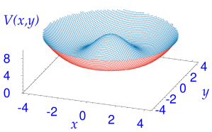
Figure 1: Mexican hat potential $V(x,y)$ of (8) with $B=10$.

The wave-function $\psi(x,y,t)$ is intrinsically complex. For a stationary state $\psi(x,y,t)\sim\psi(x,y)e^{-{\mbox{i}}\mu t}$, where $\mu$ is the chemical potential. To write a real expression for the energy from the complex wave function $\psi(x,y)$, it is convenient to write two coupled non-linear equations for the real and imaginary parts of the wave function [32]

$$\psi=\psi_{R}+\mathrm{i}\psi_{I}\equiv\sqrt{\psi_{R}^{2}+\psi_{I}^{2}}\exp(i\varphi),$$ (9)

where $\varphi$ is the phase of the wave function. The equation satisfied by the real part is

$$\mu\psi_{R}(x,y) = \left[-\frac{1}{2}\nabla^{2}+V(x,y)+g|\psi({x,y};t)|^{2}\right]\psi_{R}({x,y};t)$$ (10)

$$+ \Omega\left(y\frac{\partial}{\partial x}-x\frac{\partial}{\partial y}\right)\psi_{I}({x,y};t)\,.$$

In this equation $\psi_{R}$ is not normalized to unity. Using  (10), the energy per atom for a stationary state in the rotating frame can be expressed as [32]

$$E(\Omega) = \frac{1}{\int dxdy\psi_{R}^{2}}\int dxdy\biggr{[}{\frac{1}{2}{(\nabla\psi_{R})^{2}}}+V(x,y)\psi_{R}^{2}$$ (11)

$$+ \frac{1}{2}g(\psi_{R}^{2}+\psi_{I}^{2}){\psi_{R}^{2}}+\Omega\psi_{R}\left(y\frac{\partial}{\partial x}-x\frac{\partial}{\partial y}\right)\psi_{I}\biggr{]},$$

Equation (11) involves algebra of real functions only and will be used in numerical calculation.

3 Numerical Results

The quasi-2D mean-field equation (2) cannot be solved analytically and we employ the split time-step Crank-Nicolson method [28, 31] for its numerical solution using a space step of 0.05 and a time step of 0.0002 for imaginary-time simulation and 0.0001 for real-time simulation. The imaginary-time propagation is used to obtain the lowest-energy stationary ground state and the real-time propagation is used to study the dynamics. There are different C and FORTRAN programs for solving the GP equation [28, 31] and one should use the appropriate one. The programs of [28] have recently been adapted to simulate the statics and dynamics of a rotating BEC [32] and we use these in this letter. Without considering a specific atom, we will present the results in dimensionless units for different sets of parameters: $\Omega,g$. In the phenomenology of a specific atom, the parameter $g$ can be varied experimentally through a variation of the underlying atomic scattering length by the Feshbach resonance technique [33].

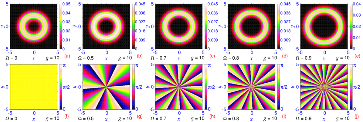
Figure 2: Giant vortex in a rotating quasi-2D BEC, trapped by the potential (8) with $B=10$, with $g=10$, satisfying (2), from a contour plot of 2D density $(|\psi|^{2})$ for $\omega$ = (a) 0, (b) 0.5, (c) 0.7, (d) 0.8 and (e) 0.9. The plots in (f)-(j) display the corresponding phase profiles $\varphi=\arctan(\psi_{I}/\psi_{R})$ of the rotating BECs illustrated in (a)-(e), respectively. All quantities plotted in this and following figures are dimensionless.

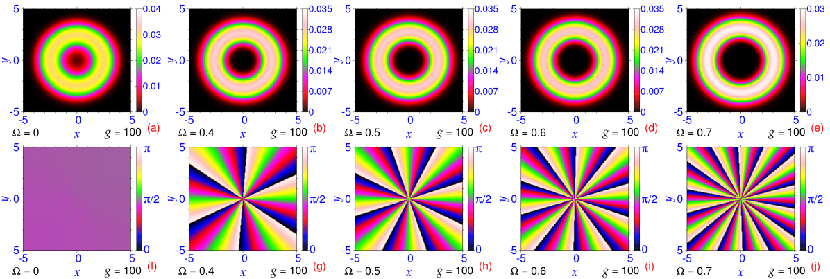
Figure 3: Giant vortex in a rotating quasi-2D BEC, trapped by the potential (8) with $B=10$, with $g=100$, satisfying (2), from a contour plot of 2D density $(|\psi|^{2})$ for $\Omega$ = (a) 0, (b) 0.4, (c) 0.5, (d) 0.7 and (e) 0.9. The plots in (f)-(j) display the corresponding phase profiles of the rotating BECs illustrated in (a)-(e), respectively.

We study how a giant vortex in a BEC trapped by the Mexican hat potential (8) with $B=10$ evolve with the increase of angular frequency of rotation $\Omega$. First we consider a small value of atomic interaction strength $g$ $(=10)$ and solve (2) increasing $\Omega$ gradually from 0 to 0.95. In all cases a clean giant vortex is generated with the angular momentum increasing gradually from 0 to 11 as $\Omega$ is increased. By the term “clean giant vortex” we mean that there is no associated vortex of unit angular momentum in the body of the giant vortex. The angular momentum in the giant vortex is obtained from an analysis of phase of the wave function. In Figs. 2(a)-(j) we plot the density ($|\psi|^{2}$) of the rotating BEC for different $\Omega$ and the associated phase $(\varphi)$ of the wave function, viz. (9). A jump of phase of $2\pi$ along a closed path $\cal C$ around the center correspond to a unit angular momentum, viz. (1). The angular momenta of the generated giant vortex for $\omega=0,0.5,0.7,0.8$ and 0.9 are $l=$ 0, 3, 6, 7 and 11, respectively. The phases of figure 2 confirm that we really have a single giant vortex of large angular momentum and not several vortices with a large total angular momentum: this is because the phase jump takes place around a single isolated central point. By increasing $\Omega$ in small steps we can easily generate a giant vortex with an intermediate value for angular momentum, e.g., $l=$ 2, 4, 5, 8, 9, 10 etc. not shown in figure 2.

We now consider the effect of increasing the atomic interaction strength $g$. For this purpose we consider the evolution of the giant vortex for $g=100$. The numerically obtained density and the related phase profile in this case are illustrated in figure 3 for $\Omega=0$, 0.4, 0.5, 0.6 and 0.7 in plots (a)-(e) and (f)-(j), respectively. In this case, for values of $\Omega$ up to $\Omega=0.7$, a clean giant vortex with a large angular momentum is obtained. The angular momentum of the giant vortex for $\Omega=0,0.4,0.5,0.6$ and 0.7 are 0, 3, 4, 5 and 7, respectively, as illustrated in figure 3. It is interesting to consider the fate of the giant vortex for larger interaction strength $g$ and $\Omega$. For $g=100$ and for larger $\Omega(\gtrapprox 0.75)$ vortices of unit angular momentum are also generated inside the body of the giant vortex with a large angular momentum. This is illustrated in figure 4. The density and phase profile shown in figures 4(a) and (b) for $\Omega=0.9,g=100$ are qualitatively different from those obtained for smaller $\Omega$ and $g$. In this case we have 11 vortices of unit angular momentum embedded in the body of the giant vortex of angular momentum of 10 units, corresponding to a total angular momentum of 21 units. We find that a clean giant vortex can be generated in a trapped BEC with $g=10$ for $\Omega\lessapprox 0.95$; for $g=100$ the same can be generated for $\Omega\lessapprox 0.75$. For $g=200$ we find that the same can be generated for $\Omega\lessapprox 0.55$ only. This is illustrated in figures 4(c)-(f) by plots of density and phase for $g=200$ and $\Omega=0.5$ and 0.75. We find, from figures 4(c)-(d), that, for $\Omega=0.5,g=200$, a clean giant vortex is generated with an angular momentum of 4 units, while, from figures 4(e)-(f), we find that, for $\Omega=0.75,g=200$, 6 unit vortices are embedded in a giant vortex of angular momentum 5. For $g>350$ no giant vortex can be generated for any $\Omega<1$ for trapping potential $(\ref{eq5})$ with $B=10$.

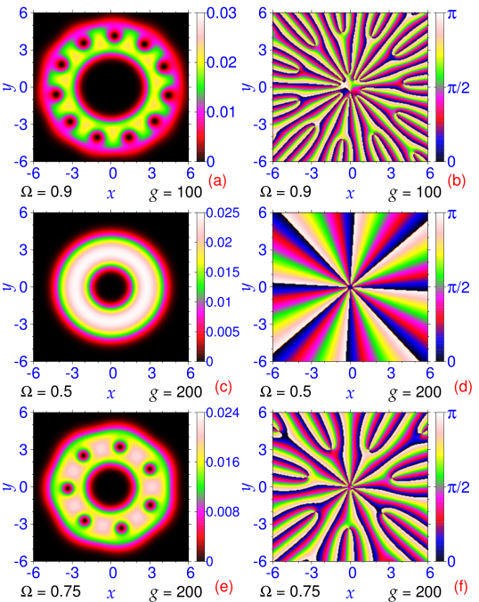
Figure 4: Giant vortex in a rotating quasi-2D BEC, trapped by the potential (8) with $B=10$ satisfying (2), from a contour plot of 2D density $(|\psi|^{2})$ for (a) $\Omega=0.9,g=100$, (c) $\Omega=0.5,g=200$, and (e) $\Omega=0.75,g=200$. The plots in (b), (d) and (f) display the corresponding phase profiles of the rotating BECs illustrated in (a), (c) and (e), respectively.

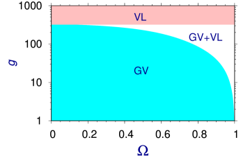
Figure 5: A $g-\Omega$ phase plot showing the domain of formation of clean giant vortex (GV), giant vortex with embedded vortex lattice (GV+VL) and only vortex lattice with no giant vortex (VL) for the trapping potential (8) with $B=10$.

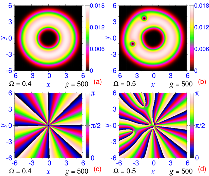
Figure 6: Giant vortex in a rotating quasi-2D BEC, trapped by the potential (8) with $B=20$ satisfying (2), from a contour plot of 2D density $(|\psi|^{2})$ for (a) $\Omega=0.4,g=500$ and (b) $\Omega=0.5,g=500$. The plots in (c), (d) display the corresponding phase profiles of the rotating BECs illustrated in (a), (b), respectively.

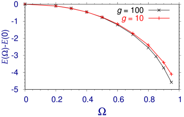
Figure 7: The rotational energy in the rotating frame $E(\Omega)-E(0)$ versus $\Omega$ for interaction strength $g=10$ and 100. The parameter $B$ of the trapping potential (8) is taken as $B=10$ in both cases.

A phase plot in the parameter space $g-\Omega$, illustrating the domains of the formation of a clean giant vortex, a giant vortex with embedded vortex lattice, and only vortex lattice with no associated giant vortex, is exhibited in figure 5. From this figure we find that, for trapping potential (8) with $B=10$, it is not possible to have a giant vortex for $g>350$. However, it is possible to have a giant vortex for a larger $g$ provided we increase the height of the hill $B$ of potential (8). For example, for $B=20$, it is possible to generate a clean giant vortex for $g=500$ as illustrated in figure 6, where we show the density and phase of the generated giant vortex for $g=500,B=20$ and $\Omega=0.4$ and 0.5. For $\Omega=0.4$, we have a clean giant vortex with angular momentum of 4 units as we see from plots (a) and (c). For $\Omega=0.5$, we have two vortices of unit angular momentum embedded in the body of a giant vortex of angular momentum of 5 units. Hence the domain of the giant vortex formation in the $g-\Omega$ phase plot of figure 5 can be augmented by increasing the parameter $B$ in potential (8).

The $\Omega$-dependent part of energy per atom can be obtained from a theoretical estimate of Fetter [5]:

$$E(\Omega)-E(0)\approx-\frac{1}{2}I\Omega^{2},$$ (12)

where $I$ is the moment of inertia of rigid-body rotation of an atom of the super- fluid. We have plotted in figure 7 this energy for $g=10$ and 100 with the trap of figure 1 with $B=10$. The energy (12) is independent of $g$ and determined only by the moment of inertia. Figure 7 confirms this universal behavior of the rotational energy.

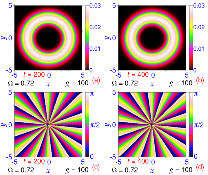
Figure 8: Dynamical evolution of a giant vortex of the rotating BEC displayed in figure 3(e), during real-time propagation for 400 units of time using the corresponding imaginary-time wave function as input, at times (a) t = 200, (b) t = 400 for density. The corresponding phases are displayed in (c) and (d). During real-time propagation the angular frequency of rotation $\Omega$ was changed at $t=0$ from the imaginary-time value of $\Omega=0.7$ to 0.72.

A giant vortex in an asymptotically harmonic trap is typically unstable [34]. The dynamical stability of the present quasi-2D giant vortex is tested next. For this purpose we subject the giant-vortex state of the rotating BEC to real-time evolution during a large interval of time using the initial stationary state as obtained by imaginary-time propagation, after slightly changing the angular frequency of rotation $\Omega$ at $t=0$. The giant vortex will be destroyed after some time, if the underlying BEC wave function were dynamically unstable. For this purpose, we consider a real-time propagation of the giant vortex exhibited in figure 3(e) for $g=100$ after changing $\Omega$ from 0.7 to 0.72 at $t=0$. The subsequent evolution of the giant vortex is displayed in figure 8 at (a) $t=200$, (b) $t=400$ for density and at (c) $t=200$, (d) $t=400$ for phase. The robust nature of the snapshots of the giant vortex during real-time evolution upon a small perturbation, as exhibited in figure 8, demonstrates the dynamical stability of the giant vortex in the quasi-2D rotating condensate.

4 Summary and Discussion

We have demonstrated the formation of a stable giant vortex in a controlled fashion, for the atomic interaction strength $g$ below a critical value, in a rotating BEC trapped by a Mexican hat potential, which is a harmonic trap modulated by a small Gaussian hill at the center. The atomic interaction strength and the rotational frequency $\Omega$ can be kept very small which will make a modeling of this phenomenology extremely accurate and reliable and hence such a giant vortex can be used in high precision studies. For atomic interaction strengths above the critical value, a giant vortex can be generated provided that the height of the central Gaussian hill is increased. Previous suggestions [17, 19, 20, 18] for the generation of a giant vortex employed a large value of $g$ and $\Omega$ or employed multi-component BECs [22] and hence the generated giant vortex could not be controlled like the present one and might not be appropriate for high precision studies. The dynamical stability of the present giant vortex was established by real-time propagation. With present experimental know-how these giant vortices can be prepared and studied in a laboratory.

References

References

- [1] Anderson M H, Ensher J R, Matthews M R, Wieman C E and Cornell E A 1995 Science 269 198 Davis K B, Mewes M O, Andrews M R, van Druten N J, Durfee D S, Kurn D M and Ketterle W 1995 Phys. Rev. Lett. 75 3969
- [2] Courteille P W, Bagnato V S and Yukalov V I 2001 Laser Phys. 11 659 Yukalov V I 2004 Laser Phys. Lett. 1 435 Dalfovo F, Giorgini S, Pitaevskii L P and Stringari S 1999 Rev. Mod. Phys. 71 463
- [3] Madison K W, Chevy F, Wohlleben W and Dalibard J 2000 Phys. Rev. Lett. 84 806 Matthews M R, Anderson B P, Haljan P C, Hall D S, Holland M J, Williams J E, Wieman C E and Cornell E A 1999 Phys. Rev. Lett. 83 3358
- [4] Abrikosov A A 1957 Zh. Eksp. Teor. Fiz. 32 1442 [Eng. Transla. 1957 Sov. Phys.-JETP 5 1174]
- [5] Fetter A L 2009 Rev. Mod. Phys. 81 647
- [6] Yarmchuk E J and Packard R E 1982 J. Low Temp. Phys. 46 479
- [7] Abo-Shaeer J R, Raman C, Vogels J M and Ketterle W 2001 Science 292 476 Abo-Shaeer J R, Raman C and Ketterle W 2002 Phys. Rev. Lett. 88 070409 Haljan P C, Anderson B P, Coddington I and Cornell E A 2001 Phys. Rev. Lett. 86 2922
- [8] Gross E P 1961 Nuovo Cimento 20 454 Pitaevskii L P 1961 Zh. Eksp. Teor. Fiz. 40 646 [Eng. Transla. 1961 Sov. Phys. JETP 13 451]
- [9] Adhikari S K and Salasnich L 2018 Scientific Rep. 8 8825
- [10] Schweikhard V, Coddington I, Engels P, Tung S and Cornell E A 2004 Phys. Rev. Lett. 93 210403
- [11] Kishor Kumar R, Tomio L, Malomed B A and Gammal A 2017 Phys. Rev. A 96 063624 Ghazanfari N, Keleş A and Oktel M Ö 2014 Phys. Rev. A 89 025601
- [12] Kasamatsu K and Sakashita K 2018 Phys. Rev. A 97 053622
- [13] Leanhardt A E, Shin Y, Kielpinski D, Pritchard D E and Ketterle W 2003 Phys. Rev. Lett. 90 140403
- [14] Su S-W, Hsueh C-H, Liu I-K, Horng T-L, Tsai Y-C, Gou S-C, and Liu W M 2011 Phys. Rev. A 84 023601 Cipriani M and Nitta M 2013 Phys. Rev. Lett. 111 170401
- [15] Adhikari S K 2019 Commun. Nonlinear Sci. Numer. Simulat. 71 212
- [16] Mason P and Aftalion A 2011 Phys. Rev. A 84 033611
- [17] Engels P, Coddington I, Haljan P C, Schweikhard V and Cornell E A 2003 Phys. Rev. Lett. 90 170405
- [18] Simula T P, Penckwitt A A and Ballagh R J 2004 Phys. Rev. Lett. 92 060401
- [19] Fetter A L, Jackson B and Stringari S 2005 Phys. Rev. A 71 013605 Kasamatsu K, Tsubota M and Ueda M 2002 Phys. Rev. A 66 053606
- [20] Aftalion A and Danaila I 2003 Phys. Rev. A 69 033608
- [21] Cozzini M, Jackson B and Stringari S 2006 Phys. Rev.A 73 013603
- [22] Qin J, Dong G and Malomed B A 2016 Phys. Rev. A 94 053611 Li Y, Chen Z, Luo Z, Huang C, Tan H, Pang W and Malomed B A 2018 Phys. Rev.A 98 063602 Kuopanportti P, Orlova N V and Milošević M V 2015 Phys. Rev. A 91 043605 Dong B, Sun Q, Liu W-M, Ji A-C, Zhang X-F and Zhang S-G 2017 Phys. Rev. A 96 013619 Xu X-Q and Han J H 2011 Phys. Rev. Lett. 107 200401
- [23] Grimm R, Weidemüller M, Ovchinnikov Y B 2000 Adv. At. Mol. Opt. Phys. 42 95 He X, Yu S, Xu P, Wang J and Zhan M 2012 Opt. Express 20 3711
- [24] Onsager L 1949 Nuovo Cimento. 6 249, supp 2
- [25] Feynman R P 1955 Prog. Low Temp. Phys. 1 17
- [26] Sonin E B 2016 Dynamics of Quantised Vortices in Superfluids (Cambridge, Cambridge University Press)
- [27] London F 1938 Nature 141 643
- [28] Muruganandam P and Adhikari S K 2009 Comput. Phys. Commun. 180 1888 Vudragović D, Vidanović I, Balaž A, Muruganandam P and Adhikari S K 2012 Comput. Phys. Commun. 183 2021 Young-S. L E, Muruganandam P, Adhikari S K, Lončar V, Vudragović D and Balaž A 2017 Comput. Phys. Commun. 220 503 Young-S. L E, Vudragović D, Muruganandam P, Adhikari S K and Balaž A 2016 Comput. Phys. Commun. 204 209
- [29] Landau L D and Lifshitz E M 1960 Mechanics (Oxford, Pergamon Press) section 39
- [30] Salasnich L, Parola A and Reatto L 2002 Phys. Rev. A 65 043614
- [31] Lončar V, Balaž A, Bogojević A, Skrbić S, Muruganandam P and Adhikari S K 2016 Comput. Phys. Commun. 200 406 Satari´c B, Slavnić V, Belić A, Balaž A, Muruganandam P and Adhikari S K 2016 Comput. Phys. Commun. 200 411
- [32] Kishor Kumar R, Lončar V, Muruganandam P, Adhikari S K and Balaž A 2019 Comput. Phys. Commun. 240 74
- [33] Inouye S, Andrews M R, Stenger J, Miesner H-J, Stamper-Kurn D M and Ketterle W 1998 Nature 392 151
- [34] Kuopanportti P and Möttönen M 2010 Phys. Rev.A 81 033627 Kuopanportti P and Möttönen M 2010 J. Low Temp. Phys. 161 561