Pulse shaping by a frequency filtering of a sawtooth phase-modulated CW laser

Abstract

The spectrum of a CW field whose phase experiences a periodic sawtooth modulation is analyzed. Two types of the sawtooth phase modulation are considered. One is created by combining many harmonics of the fundamental frequency. The second is produced by electro-optic modulator fed by the relaxation oscillator, which generates a voltage slowly rising during charging the energy storage capacitor and dropping fast due to discharge by a short circuit. It is proposed to filter out the main spectral component of the sawtooth phase modulated field. This filtering produces short pulses from CW phase modulated field. Several filters are proposed to remove the selected spectral component. It is shown that such a filtering is capable to produce a train of short pulses. Duty cycle of this train is equal to the modulation period and duration of the pulses can vary from $10^{-1}$ to $10^{-2}$ of the period. Depending on the modulation frequency, the proposed method is capable to produce pulses with duration ranging from nanoseconds to a fraction of picosecond.

I Introduction

Ultrafast optics is applied in widespread domains including but not limited to high-field laser matter interactions, ultrafast time-resolved spectroscopy, high precision frequency metrology and development of optical clocks, nonlinear microscopy, optical communications, see for example Refs. Book1 ; Book2 . Initially, short periodic pulses are generated by high-repition-rate mode-locked lasers. However, in this method the generated pulses and their corresponding spectral lines can suffer from instability problems. Alternative passive systems generating pedestal-free optical pulses with high peak power from a low-power laser employ large variety of methods to compress the pulses. Among them one can mention, for example, acousto-optic modulators (AOM) Warren1 ; Warren2 ; Verluise , frequency chirping followed by dispersive compensators Treacy ; Grischkowsky1974 ; Pearson ; Nakatsuka ; Nikolaus , dispersive modulators Loy1 ; Loy2 , high r.f. power spatial modulation of the field phase by electro-optic modulators (EOM) followed by a lens Kobayashi2005 , and modification of phases and amplitudes of the spectral components of the phase modulated field by the programmable filters to engineer the desired spectrum of the field Weiner2011 . Passive systems using phase modulated CW laser offer several advantages. Among them are lower cost and complexity, easy tuning of the frequency comb offset, continuous tunability of the duty cycle, and reasonably stable operation without active control. Phase modulating techniques, mentioned above, are based on the phase manipulation of the spectral components of the frequency comb, which makes phasing of these components. Therefore, duration of the compressed pulses shortens with increase of the value of the phase modulation index, while duty cycle is always equal to the modulation period.

A different method of pulse compression was recently reported in Vagizov ; Shakhmuratov2015 ; Shakhmuratov2017 ; Kocharovskaya2018 . The capabilities of this method was experimentally demonstrated for gamma photons with long duration of a single-photon wave packet Vagizov ; Shakhmuratov2015 . Splitting of a single-photon long pulse into short pulses can be used to create time-bin qubits, whose concept was introduced before in quantum informatics for optical photons Gisin1999 ; Gisin2002 .

The method Vagizov ; Shakhmuratov2015 is also based on frequency modulation of the radiation field. However, in spite of subsequent phasing of the produced spectral components, absorption (removal) of a particular spectral component is used Vagizov ; Shakhmuratov2015 ; Shakhmuratov2017 . This removal method has many in common with other methods used before. The method is also flexible and allows fine control of the duration and repetition rate of the pulses. An appreciable shortening of the pulses Shakhmuratov2015 ; Shakhmuratov2017 is achieved for high phase-modulation index as in the previous passive methods of the pulse shaping.

In this paper, new modification of the phase modulation with subsequent removal of the one of the spectral components of the comb is proposed. In this variant, appreciable pulse compression can be achieved for moderate value of the modulation index, which is even smaller than that produced by EOM fed by the half-wave voltage $V_{\pi}$.

The core idea of the method is a sawtooth phase modulation in which the phase periodically ramps upward and then sharply drops. Linear phase rise and sharp drop are proposed to construct using additive synthesis of many harmonics of frequency $\Omega$ with decreasing amplitudes according to the law $1/n$, where $n$ is the number of the harmonic $n\Omega$. The larger the number $N$ of the highest harmonic, which is $N\Omega$, the sharper the phase drop is. This simple model of the phase modulation allows to describe analytically all the details of the pulse shaping based on one spectral component removal in the spectrum of the phase modulated field. Duration of the compressed pulse, predicted by the model, is $2(2N+1)$ times shorter than the period $T=2\pi/\Omega$ of the phase modulation. Understanding of physics of this pulse shaping technique allows to extend the method to the case of nonideal sawtooth phase modulation with  periodic nonlinear phase rise and exponential phase drop. The faster the phase drops, the shorter the pulse is produced.

The sawtooth phase modulation technique is also based on the removal of one spectral component of the comb spectrum of the phase modulated field similar to the method of harmonic phase modulation Vagizov ; Shakhmuratov2015 ; Shakhmuratov2017 . This filtering is proposed to implement by cloud of cold atoms, atomic vapors, organic molecules doped in a polymer matrix, and liquid crystal phase modulator (LCM). Depending on the value of the modulation frequency and selected frequency filter, one can generate a sequence of pulses ranging from nanoseconds to a fraction of picosecond.

The paper is organized as follows. In Sec. II, a sawtooth phase modulation I, created by mixing many harmonics of the fundamental frequency, is considered. In Sec. III, frequency filtering of the phase modulated field is discussed. In Sec. IV, periodic sawtooth phase modulation, which consists of slowly rising stage according to the law $(1-e^{-t/T_{R}})$ and fast dropping stage according to $e^{-t/T_{D}}$, and frequency filtering of the phase modulated field are considered. Frequency filtering methods are discussed in Sec. V.

II Sawtooth phase modulation I

We consider CW radiation field $E(t)=E_{0}\exp(-i\omega_{r}t+ikz)$, which after passing through the electro-optic modulator acquires a sawtooth phase modulation

$$E_{EO}(t)=E(t)e^{i\varphi(t)},$$ (1)

where

$$\varphi(t)=\sum_{n=-\infty}^{+\infty}\left(\Omega t-2\pi n\right)\left\{\theta\left[t-T\left(n-\frac{1}{2}\right)\right]-\theta\left[t-T\left(n+\frac{1}{2}\right)\right]\right\},$$ (2)

$\Omega$ and $T=2\pi/\Omega$ are the modulation frequency and period, $n$ is an integer varying from $-\infty$ to $+\infty$, and $\theta(x)$ is the Heaviside step function. This kind of phase modulation is shown in Fig. 1 by dotted blue line.

Physically, it is difficult to make instantaneous phase drop after a linear ramp up. This problem can be solved by using additive synthesis of many harmonics of frequency $\Omega$ with decreasing amplitudes. Fourier transforms,

$$\frac{1}{T}\int_{-T/2}^{T/2}\varphi(t)e^{-in\Omega t}dt=i\frac{(-1)^{n}}{n},$$ (3)

for $n\neq 0$ and $\int_{-T/2}^{T/2}\varphi(t)dt=0$ for $n=0$, give the frequency content of $\varphi(t)$ for the limited number $N$ of the harmonics, i.e.,

$$\varphi_{N}(t)=2\sum_{n=1}^{N}(-1)^{n+1}\frac{\sin(k\Omega t)}{n},$$ (4)

where $N$ defines the highest frequency $N\Omega$ of the Fourier content of the synthesized periodic phase evolution. Example of $\varphi_{N}(t)$ with $N=5$ is shown in Fig. 1 by red solid line. It is interesting to notice that modulation index of the main spectral component with $n=1$ is equal $2$, while together with other four components the maximum phase shift is $\pi$, which can be produced by the half-wave voltage $V_{\pi}$ applied to EOM.

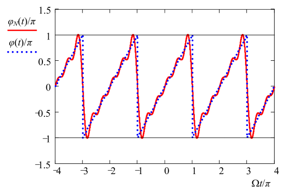
Figure 1: Time evolution of the sawtooth phase $\varphi(t)$ (blue dotted line) and the phase $\varphi_{5}(t)$, synthesized from 5 harmonics (solid red line). Both are normalized to $\pi$. Horizontal black bars show limiting values of the phase change, $\pm\pi$

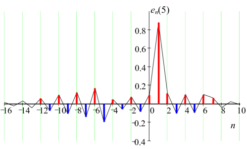
Figure 2: Frequency content of the field with sawtooth phase modulation synthesized from $N=5$ harmonics. The amplitudes of the spectral components are shown by red (positive amplitudes) and blue (negative amplitudes) bars. Their maxima are linked by black solid lines for visualization.

Fourier transform

$$\frac{1}{T}\int_{-T/2}^{T/2}e^{i\varphi_{N}(t)-in\Omega t}dt=e_{n}(N),$$ (5)

allows to find the Fourier content of the field $E_{EO}(t)=E(t)e^{i\varphi_{N}(t)}$ transmitted through AOM, which can be expressed as

$$E_{EO}(t)=E_{0}e^{-i\omega_{r}t+ikz}\sum_{n=-\infty}^{n=\infty}e_{n}(N)e^{in\Omega t}.$$ (6)

The amplitudes of the spectral components $e_{n}(N)$ are shown in Fig. 2. The component with $n=1$ has the largest amplitude. For example, for $N=5$ this amplitude is $e_{1}(5)=0.879$. With increase of $N$, this amplitude tends to $1$, i.e., $e_{1}(10)=0.936$ for $N=10$ and $e_{1}(50)=0.987$ for $N=50$. Numerical analysis shows that $e_{1}(N)$ can be approximated as $e_{1}(N)\approx 1-1.33/(2N+1)$.

The satellites of the component with $n=1$ have smaller amplitudes, and their signs change such that nearest components to the central one, which we denote as $n_{c}=1$, are positive ($n_{c}\pm 1$), the next pair ($n_{c}\pm 2$) is negative, then the next amplitudes with numbers $n_{c}\pm 3$ are positive, etc. until $n_{c}\pm N$, see Fig. 2. The amplitudes of the components in each pair are not equal, i.e., $e_{0}(5)=0.102$ and $e_{2}(5)=0.111$ for the nearest pair, $e_{-1}(5)=-0.085$ and $e_{3}(5)=-0.105$ for the next pair. With increase of $N$, the absolute values of the amplitudes of the satellites decrease, while the number of satellites with noticeable value of the amplitudes increases resulting in the spectrum broadening of the field. In addition, the amplitudes of the pairs with numbers $n_{c}\pm 1$ and $n_{c}\pm 2$ tend to be equal for large $N$, i.e., $e_{2}(50)=e_{0}(50)=0.013$ and $e_{3}(50)=e_{-1}(50)=-0.013$

Thus, sawtooth phase modulation makes a frequency offset of the CW field $E(t)$ changing its carrier frequency to $\omega_{r}-\Omega$. This is the first difference between the sawtooth phase modulation $\varphi_{N}(t)$, Eq. (4), and harmonic phase modulation $\varphi_{h}(t)=m\sin\Omega t$. The latter does not change the central frequency of the field. Here, $m$ is the modulation index of the harmonic phase modulation. The second difference between them is the qualitatively different dependence of the amplitudes of the sidebands on their numbers. The amplitudes of the harmonics $+n\Omega$ and $-n\Omega$, produced by the harmonic phase modulation, have the same sign if $n$ is even, and they have opposite signs if $n$ is odd. The amplitudes of the harmonics $(n_{c}+n)\Omega$ and $(n_{c}-n)\Omega$, produced by the sawtooth phase modulation, have always the same sign for $n\leq N$. Here, we remind that $n_{c}=1$ is the number of the central component of the frequency comb created by the sawtooth phase modulation.

III Frequency filtering of the phase modulated field I

If we selectively remove the central component $n_{c}$ of the phase modulated field without change of all other spectral components, we expect that remaining $2N$ components will phase and rephase with the period $T$. To explain this point we just consider, for example, the interference of only two nearest spectral pairs of the central components,

$$E_{tp}(t)=E(t)\left[e_{-1}(N)e^{-i\Omega t}+e_{0}(N)+e_{2}(N)e^{2i\Omega t}+e_{3}(N)e^{3i\Omega t}\right],$$ (7)

and assume that $e_{0}(N)=e_{2}(N)=-e_{-1}(N)=-e_{3}(N)=a$, which is the case when $N=50$ and $a=0.013$. Then, Eq. (7) can be expressed as

$$E_{tp}(t)=2aE(t)e^{-i\Omega t}\left(\cos\Omega t-\cos 2\Omega t\right).$$ (8)

This equation shows that when $\Omega t=2k\pi$ the amplitude $E_{tp}(t)$ is zero because of destructive interference of the spectral pair $e_{0}(N)$, $e_{2}(N)$ with the pair $e_{-1}(N)$, $e_{3}(N)$. When $\Omega t=(2k+1)\pi$ the amplitude $E_{tp}(t)$ is equal to $-4aE_{0}$ due to constructive interference of the spectral pairs. Here, $k$ is an integer.

Analysis of the interference of all the pairs of the frequency comb, which is described by Eq. (6) with removed central component $n_{c}$, is quite complicated. Essential simplification is achieved if one employs the method proposed in Refs. Shakhmuratov2015 ; Shakhmuratov2017 . It suggests to express the filtered comb as

$$E_{f}(t)=E(t)\left(\sum_{n=-\infty}^{n=\infty}e_{n}(N)e^{in\Omega t}-e_{n_{c}}(N)e^{in_{c}\Omega t}\right)$$ (9)

or

$$E_{f}(t)=E(t)\left[e^{i\varphi_{N}(t)}-e_{n_{c}}(N)e^{in_{c}\Omega t}\right].$$ (10)

Then, the intensity of the filtered field $I_{f}(t)=\left|E_{f}(t)\right|^{2}$ can be presented as

$$I_{f}(t)=I_{0}\left\{1-2e_{n_{c}}(N)\cos\left[n_{c}\Omega t-\varphi_{N}(t)\right]+e_{n_{c}}^{2}(N)\right\},$$ (11)

where $I_{0}=E_{0}^{2}$. According to this expression the evolution of the phase $\psi(t)=n_{c}\Omega t-\varphi_{N}(t)$ fully defines the interference of the spectral pairs, mentioned above. Formally, this interference can be considered as an interference of the whole comb, $E_{EO}(t)$, with the removed component whose phase is changed by $\pi$, i.e., with the field $E_{sc}(t)=-e_{n_{c}}(N)E(t)e^{in_{c}\Omega t}$. In the case of atomic or molecular filters, the field $E_{sc}(t)$ has a physical meaning. This field is coherently scattered in forward direction by atoms whose resonant frequency is $\omega_{r}-\Omega$ Shakhmuratov2015 ; Shakhmuratov2017 ; Shakhmuratov2011 ; Shakhmuratov2012 . In the case of the programmable filters Weiner2011 , the field $E_{sc}(t)$ is virtual.

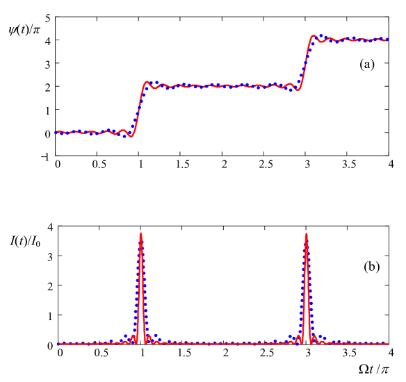
Figure 3: (a) Time evolution of the phase $\psi(t)=n_{c}\Omega t-\varphi_{N}(t)$, which specifies the interference of the comb with the scattered field $E_{sc}(t)$. (b) Time dependence of the intensity of the pulses normalized to $I_{0}$. Solid red lines correspond to the sawtooth phase modulation with $N=10$, and blue dots to $N=5$.

The scattered field $E_{sc}(t)$ is in phase with the field $E_{EO}(t)$ when $\psi(t)=(2k+1)\pi$, where $k$ is integer. Constructive interference of these fields produces a pulse with intensity $I_{\max}=I_{0}[1+e_{n_{c}}(N)]^{2}$. When $\psi(t)=2k\pi$, destructive interference of the fields results in the drop of intensity to the level $I_{\min}=I_{0}[1-e_{n_{c}}(N)]^{2}$. Substantial contrast between the pulse maximum and the pedestal is achieved if $e_{n_{c}}(N)\longrightarrow 1$. For example, for the sawtooth phase modulation, synthesized from $5$ harmonics, we have $e_{1}(5)=0.879$, which gives $I_{\min}=3.53I_{0}$ and $I_{\min}=0.015I_{0}$. Thus, for $N=5$, there is a $23.7$-dB contrast ratio between the pedestal and the pulse maximum. For $N=10$ and $N=50$, the contrast ratios are $30$ and $43.5$ dB, respectively.

Time evolution of the phase difference $\psi(t)$ of the comb $E_{EO}(t)$ and coherently scattered field $E_{sc}(t)$ is shown in Fig. 3(a) for $N=5$ and $10$. In time intervals $(k+1/2)T$ $<t<(k+3/2)T$, the phase difference $\psi(t)$ is close to $2\pi(k+1)$, which results in destructive interference of the fields. Here $k$ is an integer. On the borders of these time intervals the phase difference $\psi(t)$ jumps from $2\pi(k+1)$ to $2\pi(k+2)$ crossing the value $2\pi(k+3/2)$. At the crossing when $\psi(t)=2\pi(k+3/2)$, the pulse is formed due to constructive interference of the fields, see Fig. 3(b). The larger the number of harmonics $N$, the faster phase $\psi(t)$ crosses the value $2\pi(k+3/2)$ and the shorter pulse is formed. The slope of the phase change at the crossing point, which takes place at $t_{k}=(k+3/2)T$, is equal to $\partial\psi(t)/\partial t\mid_{t_{k}}=(2N+1)\Omega$. Thus, the rate of the crossing point is proportional to the modulation frequency $\Omega$ and the number of harmonics $N$ constituting the sawtooth phase modulation.

The phase rise at the crossing point $t_{k}$ can be approximated as a linear function $\psi(t)\approx\Omega t_{k}+(2N+1)\Omega(t-t_{k})$ with the slope $\partial\psi(t)/\partial t\mid_{t_{k}}=(2N+1)\Omega$. This function fits well the evolution of the phase $\psi(t)$ around the crossing points, see Fig. 4 where $t_{-1}$ crossing is shown. In the case $k=-1$, shown in the figure, the linear approximation is reduced to $\psi(t)\approx(2N+1)\Omega t-2\pi N$. It predicts that at $t_{-1}=T/2$ we have $\Omega t_{-1}=\pi$ and $\psi(t_{-1})=\pi$. Then, constructive interference produces a field with maximum intensity $I_{\max}=I_{0}[1+e_{n_{c}}(N)]^{2}$, which is $I_{\max}=4I_{0}$ if $e_{n_{c}}(N)\longrightarrow 1$. Neglecting the pedestal $I_{\min}=I_{0}[1-e_{n_{c}}(N)]^{2}$, one can roughly estimate from Fig. 4 that intensity of the pulse drops to its half value $I_{\max}/2$ when $t=t_{-1}\pm t_{\mathrm{half}}$ where $t_{\mathrm{half}}$ satisfies the relation $(2N+1)\Omega t_{\mathrm{half}}=\pi/2$. At times $t=t_{-1}-t_{\mathrm{half}}$ and $t=t_{-1}+t_{\mathrm{half}}$ the phase $\psi(t)$ takes the values $\pi/2$ and $3\pi/2$, respectively. Intensity of the pulse drops two times at these moments since $\cos\psi(t)$ in Eq. (11) is zero. Thus, the width of the pulse can be estimated as $2t_{\mathrm{half}}=T/2(2N+1)$, i.e., it is $(2N+1)$ time shorter than the half of the period $T=2\pi/\Omega$ of the phase modulation. Taking into account that $e_{n_{c}}(N)$ is slightly smaller than one, we numerically found that $t_{\mathrm{half}}$ satisfies slightly different relation, which is $(2N+1)\Omega t_{\mathrm{half}}=\pi/1.923$. It does not deviate significantly from our rough estimation.

IV Sawtooth phase modulation II

The sawtooth phase modulation can be also realized by EOM fed by a sawtooth voltage, which is produced by relaxation oscillators. In this type of oscillator the energy storage capacitor is charged slowly but discharged rapidly by a short circuit through the switching device. Then, the ramp vltage can be described by equation

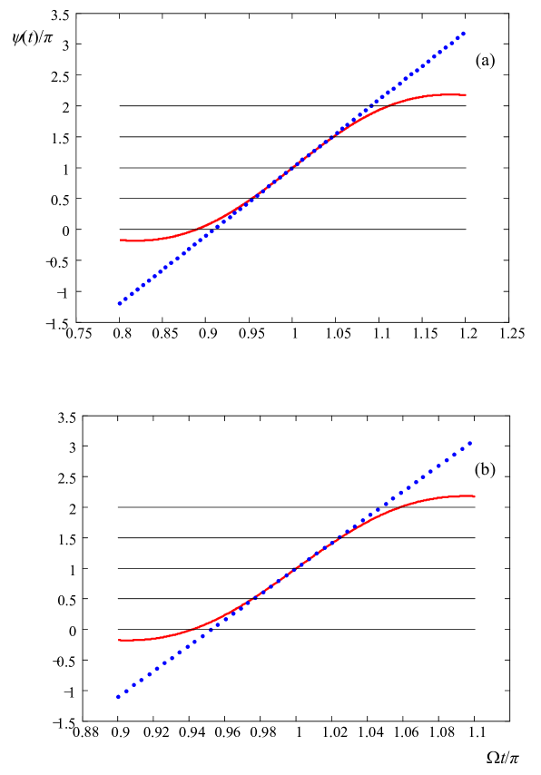
Figure 4: Time evolution of the phase $\psi(t)$ near one of the crossing points, i.e., at $t_{k}$ with $k=-1$, is shown by red solid line. Its approximation by linear time dependence is shown by blue dots (see the tex for details). The number of harmonics constituting the sawtooth phase modulation is $N=5$ in (a) and 10 in (b).

$$U_{R}(t)=U_{0}\left(1-e^{-t/T_{R}}\right)+U_{\min},$$ (12)

where $U_{0}$ is a maximum voltage, $T_{R}$ is a rise time, and $U_{\min}$ is an initial voltage, from which the ramp starts. The voltage drop is described by

$$U_{D}(t)=U_{\max}e^{-t/T_{D}},$$ (13)

where $U_{\max}$ is a voltage when the discharge starts and $T_{D}$ is a drop time.

A periodic phase modulation, produced by such a sawtooth voltage, can be expressed as follows

$$\varphi_{RO}(t)=C\sum_{k=0}^{+\infty}\phi\left[t-k\left(T_{R}+T_{D}\right)\right],$$ (14)

where

$$\phi(t)=\phi_{R}(t)+\phi_{D}(t),$$ (15)

$$\phi_{R}(t)=\left(1-e^{-t/T_{R}}\right)\left[\theta(t)-\theta(t-T_{R})\right],$$ (16)

$$\phi_{D}(t)=\left[e^{-(t-T_{R})/T_{D}}-e^{-1}\right]\left[\theta(t-T_{R})-\theta(t-T_{R}-T_{D})\right].$$ (17)

Here, for simplicity, it is assumed that the rise and drop time periods are equal to $T_{R}$ and $T_{D}$, respectively, and time independent part of the phase is disregarded resulting in the condition $\phi(0)=0$. The maximum value of the phase $\phi(t)$ at $t=T_{R}$ is taken equal to $2\pi$, which gives $C=2\pi/\left(1-e^{-t/T_{R}}\right)$. The period of this sawtooth-phase modulation is $T=T_{R}+T_{D}$. Time evolution of the phase $\varphi_{RO}(t)$ is shown in Fig. 5.

Fourier transform

$$\frac{1}{T}\int_{0}^{T}e^{i\varphi_{RO}(t)-in\Omega t}dt=c_{n},$$ (18)

allows to find the Fourier content of the field $E_{RO}(t)=E(t)e^{i\varphi_{RO}(t)}$, which is

$$E_{RO}(t)=E_{0}e^{-i\omega_{r}t+ikz}\sum_{n=-\infty}^{n=\infty}c_{n}e^{in\Omega t}.$$ (19)

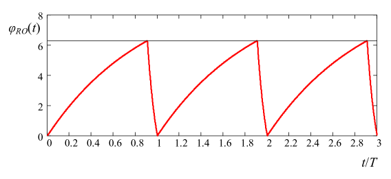
Figure 5: Time evolution of the phase $\varphi_{RO}(t)$. Time scale is normalized to $T=T_{R}+T_{D}$. The parameters of the sawtooth phase modulation are related as $T_{D}=T_{R}/10$. Black horizontal bar corresponds to $2\pi$.

where $\Omega=2\pi/T$.

Following the derivation method presented in Sec. III, one can obtain that removing of the frequency component $\omega_{r}-\Omega$, whose amplitude is $c_{1}E_{0}$, modifies the phase modulated field as

$$E_{f}(t)=E(t)\left(e^{i\varphi_{RO}(t)}-c_{1}e^{i\Omega t}\right),$$ (20)

whose intensity is

$$I_{f}(t)=I_{0}\left[1-2a_{1}\cos\psi_{RO}(t)+a_{1}^{2}\right],$$ (21)

where

$$\psi_{RO}(t)=\Omega t+\xi_{1}-\varphi_{RO}(t).$$ (22)

Here $a_{1}$ and $\xi_{1}$ are the modulus and argument (phase) of the complex number $c_{1}$, i.e. $c_{1}=a_{1}\exp(i\xi_{1})$.

Example of the formation of pulses is shown in Fig. 6(a) by blue dotted line for the case when the phase drop is ten times faster than the phase rise, i.e., for $T_{D}=T_{R}/10$. In this case $a_{1}=0.892$ and $\xi_{1}=0.808\approx\pi/3.9$. Absolute value $a_{1}$ of $c_{1}$ is close to unity. Therefore the peak pulse intensity is $3.58$ (almost four) times larger than the intensity of the CW field $I_{0}$. Evolution of the phase $\psi_{RO}(t)$, which governs the interference of the incident field, $E_{EO}(t)$, with scattered field, $E_{sc}(t)=-c_{1}E(t)e^{i\Omega t}$, is shown in Fig. 6(a) by red solid line. Each time when $\psi_{RO}(t)$ crosses the value $(2k+1)\pi$, the pulse is formed.

Zoom in on the area of the pulse formation around $t=T$ is shown in Fig. 6(b). Numerical analysis gives an estimation of the pulse duration $t_{p}$ (full width at half maximum), which is $0.041T_{R}$ for $T_{D}=T_{R}/10$. Thus, during a short time of the phase drop $T_{D}$, the pulse is mainly formed within the time interval $0.41T_{D}$, which is slightly less than a half of $T_{D}$.

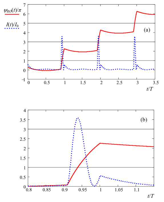
Figure 6: (a) Time evolution of the phase $\varphi_{RO}(t)/\pi$ (in units of $\pi$) is shown by red solid line. Sequence of pulses, generated by the frequency filtering, is shown by blue dotted line. The field intensity is normalized to $I_{0}$. Time scale is in units of the period $T$. Both plots correspond to the case when $T_{D}=T_{R}/10$. (b) Zoom in on the area of the pulse formation around $t=T$. In both plots, horizontal black thin lines indicate the levels corresponding to the phase values equal to $(2k+1)\pi$.

V Frequency filtering methods

Removal of the selected spectral component of the frequency comb, created by the sawtooth phase modulation I and II, can be implemented by resonant filters with a single absorption line $L(\omega-\omega_{f})$ centered at frequency $\omega_{f}$. The width of this line, $\Gamma$, is to be much smaller than the distance $\Omega$ between the frequency components of the comb, i.e. $\Gamma\ll\Omega$.

If the line is homogeneously broadened, then optically thick absorber filters out the selected frequency component $E_{s}(t)=E_{s}e^{-i\omega_{s}t+ikr}$ diminishing its amplitude as follows, see Refs. Shakhmuratov2017 ; Crisp ,

$$E_{fs}=\exp\left[-\frac{\alpha_{B}l}{2}L(\omega_{s}-\omega_{f})\right]E_{s},$$ (23)

where

$$L(\omega_{s}-\omega_{f})=\frac{\Gamma/2}{\Gamma/2-i(\omega_{s}-\omega_{f})}$$ (24)

is the Lorentzian profile describing the absorption and dispersion in the filter of physical thickness $l$ and Beer’s law absorption coefficient $\alpha_{B}$. Here, $\Gamma$ is a width at half-maximum of the Lorentzian absorption line of a single particle in the absorber. In exact resonance ($\omega_{s}=\omega_{f}$), the amplitude of the selected line decreases as $E_{fs}=\exp\left(-d/2\right)E_{s}$, where $d=$ $\alpha_{B}l$ is the optical thickness of the filter. The filtering becomes effective if $d/2\gg 1$. However, there is a limit set to the optical thickness of the filter by the condition that the spectral components $\omega_{s}\pm\Omega$ neighboring the selected component $\omega_{s}$ must be unaffected. This condition is satisfied, if $d\ll 4\Omega/\Gamma$, see Ref. Shakhmuratov2017 . The amplitudes of the neighboring components, $E_{s\pm 1}$, are changed according to the equation

$$E_{fs\pm 1}=\exp\left[-\frac{d}{2}L(\pm\Omega)\right]E_{s\pm 1}.$$ (25)

If $\Omega\gg\Gamma$, this change is mainly caused by the phase factor $\exp(\pm id\Gamma/4\Omega)$ since $-\frac{d}{2}L(\pm\Omega)$ in the exponent is approximated as $\pm id\Gamma/4\Omega$. The condition $d\ll 4\Omega/\Gamma$ allows avoiding the modification of the neighboring components of the field spectrum.

If $\omega_{s}=\omega_{f}$ and only the selected frequency component is affected by the resonant filter, then Eq. (10), describing in Sec. III the filtered comb in the ideal case of $100\%$ removal/filtering, is modified as

$$E_{f}(t)=E(t)\left[e^{i\varphi_{N}(t)}-e_{n_{c}}(N)\left(1-e^{-d/2}\right)e^{in_{c}\Omega t}\right].$$ (26)

In a similar way, Eq. (20) in Sec. IV is modified in the case of the resonant filter.

If absorption line in the filter is Doppler broadened, then the function $L(\omega-\omega_{f})$ in Eq. (25) is replaced by

$$F_{D}(\omega-\omega_{f})=\sqrt{\frac{\ln 2}{\pi}}\frac{1}{\Delta\omega_{D}}\int_{-\infty}^{+\infty}L(\omega-\omega_{f}+\omega)e^{-\ln 2\left(2\omega/\Delta\omega_{D}\right)^{2}}\omega,$$ (27)

where $\Delta\omega_{D}$ is the Doppler width, which is supposed to be much larger than $\Gamma$. At exact resonance we have $F_{D}(0)=\sqrt{\pi\ln 2}\Gamma/\Delta\omega_{D}$. Then, the amplitude of the component filtered by the absorber with inhomogeneously broadened line decreases as $E_{fs}=\exp[-dF_{D}(0)/2]E_{s}$. The neighboring components are not affected if $\Omega\gg\Delta\omega_{D}$. However, because for $\Gamma/\Delta\omega_{D}=10^{-2}$ and $\Omega>1.8\Delta\omega_{D}$ the function $F_{D}(\omega-\omega_{f})$ has Lorentzian wings Shakhmuratov2008 , i.e., it becomes $F_{D}(\omega-\omega_{f})=(\Gamma/2)/[(\Gamma/2)-i(\omega-\omega_{f})]$, their influence on the spectral neighbors of the filtered component is negligible if $d\ll 4\Omega/\Gamma$. Thus, effective filtering takes place if $\Omega\gg\Delta\omega_{D}$ and optical thickness satisfies the condition $1.35\Delta\omega_{D}/\Gamma\ll d\ll$ $4\Omega/\Gamma$, see Ref. Shakhmuratov2017 .

The filtering of the selected spectral component can be also implemented by the method based on spectral line-by-line pulse shaper, see, for example, Ref. Weiner1 . Many-pixel liquid crystal modulator (LCM) array allows in this technique to control both amplitude and phase of individual spectral lines of the field with a comb spectrum. LCM can be tuned such that only selected spectral line of the comb is suppressed.

Effective and flexible method of creating nanosecond pulses can be implemented by filtering of the frequency comb through laser-cooled atoms with a modest optical depth. For example, $D_{1}$-line transition ($\lambda=795$ nm) of ⁸⁵Rb atoms in a two-dimensional magneto-optical trap have almost homogeneous width $\Gamma\approx 6$ MHz, see, for example, Ref. Chen . Therefore, with the modulation frequency of EOM $\Omega=30$ MHZ one can generate $1.5$ ns pulses for the sawtooth phase modulation I with $N=5$ and $1.24$ ns for the sawtooth phase modulation II with $T_{D}=T_{R}/10$ by the filtering through the cloud of laser-cooled ⁸⁵Rb atoms. For $N=10$, pulse duration shortens to $800$ ps. If the modulation frequency is increased to $\Omega=300$ MHZ, then the duration of the generated pulses is shortened to $150$ ps for $N=5$ and to $80$ ps for $N=10$. For the sawtooth phase modulation II with $T_{D}=T_{R}/10$ pulses shorten to $124$ ns.

As a frequency filter one can use a vapor of ⁸⁷Rb atoms. Assume that the selected frequency of the comb is tuned in resonance with the $S_{1/2},F=1\rightarrow P_{1/2},F=2$ transition of the $D_{1}$ line of natural Rb ($\lambda=795$ nm). Below, we take the parameters of the experiment Lukin where spectral properties of the electromagnetically induced transparency were studied in this vapor. Natural linewidth of the Rb $D_{1}$ line is $\Gamma=5.4$ MHz and Doppler broadening is $\Delta\omega_{D}=500$ MHz. Selecting the phase modulation frequency $\Omega=10$ GHz, which is 20 times larger than the Doppler width $\Delta\omega_{D}=500$ MHz, we satisfy the condition $\Omega\gg\Delta\omega_{D}$. According to the estimates given in Ref. Shakhmuratov2017 for the Rb cell with the length $l=5$ cm and atomic density $N_{1}=6\times 10^{10}$ cm^-3, the modification of the spectral components neighboring the selected one is almost negligible. For this atomic density the effective optical depth of the cell at the selected line center is $dF_{D}(0)=14.4$ while $d=905$. With these values of the parameters $\Omega$, $\Delta\omega_{D}$, $\Gamma$, and $d$ the condition $1.35\Delta\omega_{D}/\Gamma\ll d\ll$ $4\Omega/\Gamma$ is easily satisfied.

For the modulation frequency $\Omega=10$ GHz, filtering through the atomic vapor or removing of the selected spectral component with the help of LCM Weiner1 produce much shorter pulses. For example, for the sawtooth phase modulation I with $N=5$ and sawtooth phase modulation II with $T_{D}=T_{R}/10$ one can generate $4.5$ and $3.7$ ps pulses, respectively. For the sawtooth phase modulation I consisting of 10 harmonics ($N=10$), duration of the pulses shortens to $2.4$ ps. If the number of the harmonics increases to $N=50$, pulse duration shortens to $495$ fs.

As a selective filter one can use organic molecules doped in polymer matrix. It is experimentally possible to burn a broad spectral hole in their spectrum with a sharp absorption peak sitting at its center. Such a structure is persistent at liquid helium temperature. The frequency resolution of the persistent spectral hole burning is limited by the width of the homogeneous zero-phonon line of the chromophore molecules, which typically has a width of $10^{-2}-10^{-4}$ cm^-1 or less Rebane1995 ; Rebane2002 . The holes could be burned in a planar waveguide geometry where a thin polymer film with doped molecules is superimposed as a cover layer on a planar glass waveguide Tschanz1995 ; Tschanz1996 . Then, illumination in the transverse direction with low absorption creates a hole, while weak probing field propagates in a longitudinal wave guiding direction with high absorption. For example, such a waveguide with a spectral hole acting as subgigahertz narrow-band filter was proposed to observe slow light phenomenon in Refs. Shakhmuratov2005 ; Rebane2007 .

VI Conclusion

Pulse shaping by the spectral line pulse shaper is capable to produce short pulses from the CW phase modulated field. Harmonic phase modulation with a single frequency produces pulses or bunches of pulses with the duty factor equal to the modulation period. Duration of the pulses shortens with increase of the phase modulation index. Liquid crystal phase modulator (LCM) can produce pulses whose duration is an order of magnitude shorter than the modulation period if $\sim 10$ spectral components with noticeable amplitudes are phased by LCM. Removal of the selected spectral component is also capable to produce pulses of comparable duration. However, as the LCM method, it produces such a short pulses if modulation index is larger than $\pi$. Moreover, with increase of the modulation index the contrast between the pedestal and pulse maximum decreases in the removal method. Pulse shaping by the removal of the selected spectral component of the CW sawtooth phase modulated field works with the fixed modulation index of moderate value. Short pulses are generated during fast dropping of the phase. The faster this drop is, the shorter the pulse is formed. Its duration can made an order or two orders of magnitude shorter than the phase modulation period. The contrast between the pedestal and the pulse maximum increases with increase of the rate of the phase drop.

VII Acknowledgments

This work was funded from the government assignment for FRC Kazan Scientific Center of RAS

References

- (1) A. M. Weiner, Ultrafast Optics, Wiley, Hoboken, NJ, 2009.
- (2) J. C. Diels, W. Rudolph, Ultrashort Laser Pulse Phenomena, 2nd ed. Academic Press, San Diego, 2006.
- (3) C. W. Hillegas, J. X. Tull, D. Goswami, D. Strickland, and W. S. Warren, Opt. Lett. 19, 737 (1994).
- (4) M. R. Fetterman, D. Goswami, D. Keusters, W. Yang, J.-K. Rhee, and W. S. Warren, Opt. Express 3, 366 (1998).
- (5) F. Verluise, V. Laude, Z. Cheng, Ch. Spielmann, and P. Tournois, Opt. Lett. 25, 575 (2000).
- (6) E. B. Treacy, Phys. Lett. A 28, 34 (1968).
- (7) D. Grischkowsky, Appl. Phys. Lett. 25, 566 (1974).
- (8) J. E. Bjorkholm, E. H. Turner, and D. B. Pearson, App. Phys. Lett. 26, 564 (1975).
- (9) H. Nakatsuka, D. Grischkowsky, and A. C. Balant, Phys. Rev. Lett. 47, 910 (1981).
- (10) B. Nikolaus, D. Grischkowsky, Appl. Phys. Lett. 42, 1 (1983).
- (11) M. T. Loy, App. Phys. Lett. 26, 99 (1975).
- (12) M. T. Loy, IEEE Journal of Quantum Electronics QE-13, 388 (1977).
- (13) S. Hisatake, Y. Nakase, K. Shibuya, and T. Kobayashi, Opt. Lett. 30, 777 (2005).
- (14) A. M.Weiner, Optics Communications 284, 3669 (2011), special Issue on Optical Pulse Shaping, Arbitrary Wave-form Generation, and Pulse Characterization.
- (15) F. Vagizov, V. Antonov, Y. V. Radeonychev, R. N. Shakhmuratov, and O. Kocharovskaya, Nature 508, 80 (2014).
- (16) R. N. Shakhmuratov, F. G. Vagizov, V. A. Antonov, Y. V. Radeonychev, M. O. Scully, and O. Kocharovskaya, Phys. Rev. A 92, 023836 (2015).
- (17) R. N. Shakhmuratov, Phys. Rev. A 95, 033805 (2017).
- (18) I. R. Khairulin, V. A. Antonov, Y. V. Radeonychev, O. A. Kocharovskaya, J. Phys. B: At., Mol. Opt. Phys. 51, 235601 (2018).
- (19) J. Brendel, N. Gisin, W. Tittel, and H. Zbinden, Phys. Rev. Lett. 82, 2594 (1999).
- (20) I. Marcikic, H. de Riedmatten, W. Tittel, V. Scarani, H. Zbinden, and N. Gisin, Phys. Rev. A 66, 062308 (2002).
- (21) R. N. Shakhmuratov, F. G. Vagizov, and O. Kocharovskaya, Phys. Rev. A 84, 043820 (2011).
- (22) R. N. Shakhmuratov, Phys. Rev. A 85, 023827 (2012).
- (23) M. D. Crisp, Phys. Rev. A 1, 1604 (1970).
- (24) R. N. Shakhmuratov, J. Odeurs, Phys. Rev. A 78, 063836 (2008).
- (25) Z. Jiang, D. E. Leaird, and A. M. Weiner, IEEE J. Quantum Electron. 42, 657 (2006).
- (26) J. F. Chen, H. Jeong, L. Feng, M. M. T. Loy, G. K. L. Wong, and S. Du, Phys. Rev. Lett. 104, 223602 (2010).
- (27) M. D. Lukin, M. Fleischhauer, A. S. Zibrov, H. G. Robinson, V. L. Velichansky, L. Hollberg, and M. O. Scully, Phys. Rev. Lett. 79, 2959 (1997).
- (28) H. Schwoerer, D. Erni, and A. Rebane, J. Opt. Soc. Am. B 12, 1083 (1995).
- (29) A. Renn, U. P. Wild, and A. Rebane, J. Phys. Chem. 106, 3045 (2002).
- (30) M. Tschanz, A. Rebane, and U. P. Wild, Optical Engineering 34, 1936 (1995).
- (31) M. Tschanz, A. Rebane, D. Reiss, and U. P. Wild, Mol. Cryst. Liq. Crust. 283, 43 (1996).
- (32) R. N. Shakhmuratov, A. Rebane, P. Megret, and J. Odeurs, Phys. Rev. A 71, 053811 (2005).
- (33) A. Rebane, R. N. Shakhmuratov, P. Megret, and J. Odeurs, J. Lumin. 127, 22 (2007).