A non-perturbative approach to computing seismic normal modes in rotating planets

Abstract

A Continuous Galerkin method based approach is presented to compute the seismic normal modes of rotating planets. Special care is taken to separate out the essential spectrum in the presence of a fluid outer core using a polynomial filtering eigensolver. The relevant elastic-gravitational system of equations, including the Coriolis force, is subjected to a mixed finite-element method, while self-gravitation is accounted for with the fast multipole method. Our discretization utilizes fully unstructured tetrahedral meshes for both solid and fluid regions. The relevant eigenvalue problem is solved by a combination of several highly parallel and computationally efficient methods. We validate our three-dimensional results in the non-rotating case using analytical results for constant elastic balls, as well as numerical results for an isotropic Earth model from standard “radial” algorithms. We also validate the computations in the rotating case, but only in the slowly-rotating regime where perturbation theory applies, because no other independent algorithms are available in the general case. The algorithm and code are used to compute the point spectra of eigenfrequencies in several Earth and Mars models studying the effects of heterogeneity on a large range of scales.

Declarations

This research was supported by the Simons Foundation under the MATH+X program, the National Science Foundation grant DMS-1815143, the members of the Geo-Mathematical Imaging Group at Rice University, and XSEDE research allocation TG-EAR170019. The work by R.L. was performed under the auspices of the U.S. Department of Energy by Lawrence Livermore National Laboratory under Contract DE-AC52-07NA27344 (LLNL-JRNL-780818). Y.X. and Y.S. were supported by NSF-1812695.

The codes are made available via https://github.com/js1019/NormalModes and https://github.com/eigs/pEVSL. The data can be reproduced using the codes in https://github.com/js1019/PlanetaryModels. In addition, the Mars models can be found in agwx-jd58-20 , where the performance and reproducibility were studied in shi2021planetary .

1 Introduction

Planetary normal modes are instrumental for studying the dynamic response to sources including earthquakes along faults and meteorite impacts, as well as tidal forces dahlen1998theoretical ; lognonne2005planetary . The low-angular-order eigenfrequencies contain critical information about the planet’s large-scale structure and provide constraints on heterogeneity in composition, temperature, and anisotropy, while rotation constrains the shapes as well as possible density distributions of planets. The effect of rotation on the seismic point spectrum of the Earth is well understood and has been observed for decades (park2005earth, , Fig.1). The observation of spectral energy of low-frequency toroidal modes in vertical seismic recordings of the 1998 Balleny Islands earthquake zurn2000observation , is a manifestation of the three-dimensional heterogeneity and anisotropy of the mantle structures and rotation.

For a review of Earth’s free oscillations, we refer to woodhouse2007 . Current standard approaches to computing the seismic point spectrum and associated normal modes have several limitations. Assuming spherical symmetry for non-rotating planets, the problem becomes one-dimensional and the computation of normal modes in such models using MINEOS woodhouse1988calculation ; masters2011mineos is still common practice; these are then typically used in perturbation-theory and mode-coupling approaches to include lateral heterogeneities. Full-mode coupling methodology utilizing normal modes in a spherically symmetric model as a basis has been adopted to studying Earth’s interior for decades dahlen1968normal ; dahlen1969normal ; woodhouse1978effect ; woodhouse1980coupling ; park1986synthetic ; park1990subspace ; romanowicz1987multiplet ; lognonne1990modelling ; hara1991inversion ; hara1993inversion ; um1991normal ; lognonne1991normal ; deuss2001theoretical ; deuss2004iteration ; al2012calculation ; yang2015synthetic . This methodology is of Rayleigh-Ritz type, and is justified under the assumption that the space in which the normal modes lie contains the mentioned basis, which requires spherically symmetric fluid-solid and surface boundaries. Here, we remove this limitation. Moreover, a separation of the essential spectrum needs to be carefully carried out, which has been commonly ignored in the “radial” algorithms. We discuss the mode-coupling approach and the conditions under which it applies in Appendix B.

To simulate seismic waves in strongly heterogeneous media, the spectral-element method (SPECFEM) komatitsch1998spectral ; komatitsch1999introduction has been widely used for more than two decades. We mention the software package SPECFEM3D_globe komatitsch2002spectral1 ; komatitsch2002spectral2 , which is capable of modeling relatively high-frequency waveforms in an entire planet while suppressing the perturbation to the gravitational potential. Other implementations of SPECFEM chaljub2003solving ; chaljub2004spectral ; chaljub2007spectral have been developed with alternative numerical approaches pertaining to the fluid outer core. In principle, seismic eigenfrequencies show up by taking a discrete Fourier transform of numerical solutions; however, it is a major computational challenge to control the accuracy at very long time scales. We note that in SPECFEM3D_globe, the fluid displacement is replaced by a scalar potential, which results in a non-symmetric system of discretized equations. Moreover, the (square of the) Brunt-Väisälä frequency is assumed to be zero. Rotation in the fluid regions is unnaturally introduced by means of an additional vector (cf. (komatitsch2002spectral2, , (16) and (17)) and (chaljub2007spectral, , (30))). In addition, current SPECFEM3D_globe does not include the incremental gravitational field, which limits its usage for relatively higher frequency wave propagation.

One may view the computational approach developed in this paper as forming a bridge between SPECFEM3D_globe, and the mode-coupling approaches derived from modes in a spherically symmetric model, involving finer scale heterogeneity and higher seismic eigenfrequencies. Our approach facilitates the studies of the highly heterogeneous crust models and complex three-dimensional models through the planetary spectrum, as well as the naturally efficient computation of seismograms from many different sources. Naturally, we also include the Coriolis force and centrifugal potential and formulate it as a nonlinear eigenvalue problem. We can accommodate arbitrarily shaped fluid-solid boundaries which becomes increasingly important at higher rotation rates. In our formulation, the rotation rate might spatially vary, which is relevant to the future computation of normal modes in gas giants in our solar system.

In this paper, we revisit the work of buland1984computation . Buland and collaborators encountered several complications that we overcome by characterizing and separating the essential spectrum using a polynomial filtering eigensolver and introducing a new formulation that properly models the elastic-gravitational system without simplifications. In our proposed formulation, the displacement, the proper orthonormal condition and the symmetry of the system for non-rotating planets are preserved. We apply fully unstructured meshes to model fully heterogeneous planets, and the mixed finite-element method (FEM) to discretize the elastic-gravitational system. Our method can handle fully heterogeneous planetary models easily, and guarantee that accurate solutions lie in the space to which normal modes associated with the seismic point spectrum belong. In a previous paper DBLP:conf/sc/ShiLXSH18 , we introduced a highly parallel algorithm for solving the generalized eigenvalue problem resulting from our analysis for Cowling approximation using P1 mixed FEM. We achieved high parallel computational and memory scalabilities with demonstrated performance on modern supercomputers. In the following paper shi2021planetary , we extended our algorithm using P2 mixed FEM for better accuracy and discussed the reproducibility of our codes reported from several universities during the student cluster competion at the supercomputing conference.

Self-gravitation manifests itself in the incremental gravitational potential as the density changes with displacement. We utilize the Green’s solution of Poisson’s equation and treat the self-gravitation as an $N$-body problem. We then apply the fast multipole method (FMM) greengard1997new ; gimbutas2011fmmlib3d ; yokota2013fmm , which reduces the algorithmic complexity significantly, to compute both the reference gravitational and the incremental gravitational potentials. Alternatively, one can apply a finite-infinite element method zienkiewicz1983novel ; burnett1994three for modeling unbounded domain problems to approximate the far-field of Poisson’s equation. More recently, the spectral-infinite-element method gharti2018spectral has been developed to incorporate gravity. While our eigensolver DBLP:conf/sc/ShiLXSH18 only takes matrix-vector products, any suitable schemes, including FMM or infinite-element methods, can be used in our computational framework.

To include rotation in the elastic-gravitational system through the Coriolis force and the centrifugal potential, in this work, we utilize extended Lanczos vectors computed in a non-rotating planet – with the shapes of boundaries of a rotating planet and accounting for the centrifugal potential – as a truncated basis to properly facilitate reduction to one of the equivalent linear forms of the quadratic eigenvalue problem (QEP). Here, the separation of the essential spectrum comes into play again and the normal modes computed are guaranteed to lie in the appropriate space of functions. The reduced system can be solved with a standard eigensolver.

We present and validate our three-dimensional computations using constant elastic balls and an isotropic preliminary reference Earth model as non-rotating planets with standard radial codes. The computational accuracy for rotating planets is illustrated and tested but only in the regime where perturbation theory applies as no other independent algorithms are available in the general case. We use our algorithm and code to compute the point spectra of eigenfrequencies in several Earth and Mars models, acknowledging relatively low rotation rates, studying the effects of heterogeneity on a large range of scales. The Mars models are relevant to the InSight (Interior exploration using Seismic Investigations, Geodesy and Heat Transport) banerdt2013insight ; lognonne2019seis mission. It is expected that a set of eigenfrequencies is observable panning2017planned ; bissig2018detectability . Here, we select one Mars model khan2016single from the set of blind tests clinton2017preparing ; van2019preparing and combine it with the topography zuber1992mars ; smith1999global and a three-dimensional crust belleguic2005constraints ; goossens2017evidence to create a realistic Mars model. We compute the low-angular-order eigenfrequencies and study the general effects of rotation and heterogeneity combined.

The outline of this paper is as follows. In Section 2, we revisit the form and physics of the elastic-gravitational system of a rotating planet and establish the weak formulation of the system with a separation of the essential spectrum using a polynomial filtering eigensolver. In Section 3, we discuss the hydrostatic equilibrium of a rotating fluid outer core in the presence of the gravitational and the centrifugal forces. In Section 4, we introduce the Continuous Galerkin mixed FEM and obtain the corresponding matrix equations. In Section 5, we study the computation of the reference gravitational field and the perturbation of the gravitational field using the FMM. In Section 6, we validate the computational accuracy of our work for non-rotating Earth models and quantify the effect on the point spectrum from three-dimensional heterogeneity. In Section 7, we illustrate the computational accuracy of our proposed method and show several computational experiments for different planetary models, including standard Earth and Mars models as well as related effects due to rotation and a three-dimensional crust. In Section 8, we discuss the significance of our results and directions of future research.

2 The elastic-gravitational system with rotation

In this section, we present a modified elastic-gravitational system of equations of a rotating planet to deal with the separation of the essential spectrum in the weak form de2015system (see dahlen1998theoretical for the strong formulation).

2.1 Natural subdomains and computational meshes

Following the notation in de2015system , a bounded set $\tilde{X}\subset\mathbb{R}^{3}$ is used to represent the interior of the Earth, with Lipschitz continuous exterior boundary $\partial\tilde{X}$. The exterior boundary $\partial\tilde{X}$ contains fluid (ocean) surfaces $\partial\tilde{X}^{\text{F}}$ and solid surfaces $\partial\tilde{X}^{\text{S}}$. We subdivide the set $\tilde{X}$ into solid regions $\Omega^{\text{S}}$ and fluid regions $\Omega^{\text{F}}$. The fluid regions contain the liquid outer core $\Omega^{\text{OC}}$ and the oceans $\Omega^{\text{O}}$. The solid regions can be further subdivided into the crust and mantle $\Omega^{\text{CM}}$ and the inner core $\Omega^{\text{IC}}$. We use $\Sigma$ to represent the interfaces between these subregions. In summary,

$$\tilde{X}=\,\Omega^{\text{S}}\cup\Omega^{\text{F}}\cup\Sigma\cup\partial\tilde{X},\ \partial\tilde{X}=\partial\tilde{X}^{\text{S}}\cup\partial\tilde{X}^{\text{F}},\ \Omega^{\text{S}}=\Omega^{\text{CM}}\cup\Omega^{\text{IC}},\ \ \Omega^{\text{F}}=\Omega^{\text{OC}}\cup\Omega^{\text{O}}.$$

The interior interfaces can further be subdivided into three categories: interfaces between two fluid regions $\Sigma^{\text{FF}}$, interfaces between two solid regions $\Sigma^{\text{SS}}$, and interfaces between fluid and solid regions $\Sigma^{\text{FS}}$. We can subdivide $\Sigma^{\text{FS}}$ into two major interfaces: internal interfaces $\Sigma^{\text{FS}}_{\text{int}}$ and the bottom interface $\Sigma^{\text{FS}}_{\text{O}}$ of the oceans. The internal interfaces include the interfaces between the lower mantle and the outer core $\Sigma^{\text{CMB}}$, which is known as the Core-Mantle Boundary (CMB); the interface between the outer core and the inner core is denoted as $\Sigma^{\text{ICB}}$, which is known as the Inner-Core Boundary (ICB). Thus,

$$\Sigma=\Sigma^{\text{SS}}\cup\Sigma^{\text{FF}}\cup\Sigma^{\text{FS}},\ \Sigma^{\text{FS}}=\Sigma^{\text{FS}}_{\text{int}}\cup\Sigma^{\text{FS}}_{\text{O}},\ \Sigma^{\text{FS}}_{\text{int}}=\Sigma^{\text{CMB}}\cup\Sigma^{\text{ICB}}.$$

In Fig. 1, we illustrate the concepts of the main mathematical symbols for the geometry used in this work. Since a general terrestrial planet may contain multiple complex discontinuities associated with different geological and geodynamical features, utilization of a flexible, fully unstructured tetrahedral mesh would be natural. We discretize the major discontinuities using triangulated surfaces that are generated via distmesh persson2004simple and then build up the Earth model using an unstructured tetrahedral mesh via TetGen si2015tetgen . In Fig. 2, we illustrate the interfaces and meshes with one hundred thousand and one million elements. These techniques show great flexibility and can provide models with multiple resolutions. In Figs. 3, we illustrate a three-dimensional Earth model built on a tetrahedral mesh. In Fig. 3 (a), we show the Moho interface that is constructed using an unstructured triangular mesh. The color shows the depth and the black lines are the edges of the triangles. In Fig. 3 (b), we illustrate the three-dimensional $V_{P}$ model based on MIT’s mantle tomographic results burdick2017model and crust 1.0 laske2013update . The core model is based on the Preliminary Reference Earth Model (PREM) dziewonski1981preliminary .

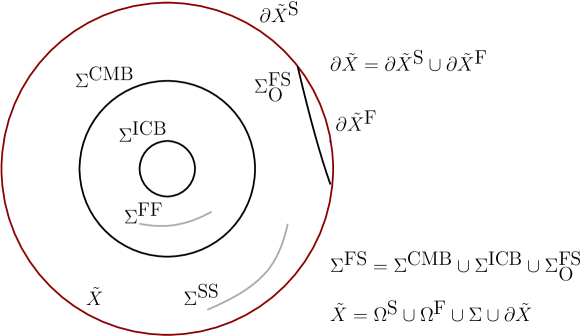
Figure 1: Conceptual figure of the geometry of a planet using Earth as an example. The red, black and grey lines indicate the outer boundary $\partial\tilde{X}$, the fluid solid boundaries $\Sigma^{\text{FS}}$, and interfaces only in the solid or fluid regions.

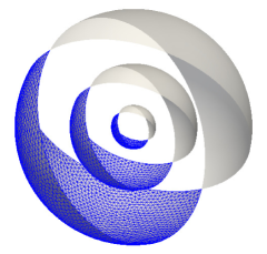
(a1)	(a2)
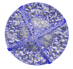
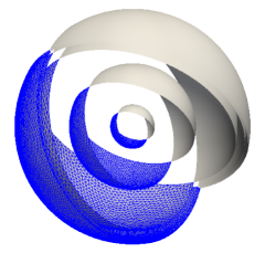
(b1)	(b2)

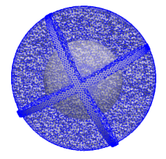
Figure 2: Illustration of different meshes. (a1) Three triangularized surface meshes; (a2) A tetrahedral mesh with 100k elements that is generated from (a1); (b1) Seven triangularized surface meshes; (b2) A tetrahedral mesh with one-million elements that is generated from (b1). The light surfaces in (b1) and (b2) denote the CMB.

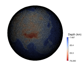
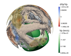
(a) Moho	(b) MIT $V_{P}$ model

Figure 3: A three-dimensional Earth model built using MIT tomographic results burdick2017model and crust 1.0 laske2013update . (a) A triangluar mesh built for the Moho interface. The color indicates the depth below the reference surface of the Earth. The bottom of the Tibet Plateau is shown. (b) MIT mantle $V_{P}$ model built on a tetrahedral mesh. The $V_{P}$ model and the contours of $\,\mathrm{d}V_{P}/V_{P}$ (%) are shown.

We also use a Mars model as an example to illustrate our construction of a terrestrial planet. The topography of Mars was measured by the Mars Orbiter Laser Altimeter (MOLA) zuber1992mars ; smith1999global with high accuracy. The thickness and density of the Martian crust were constructed with the help of the works of belleguic2005constraints ; goossens2017evidence . In Fig. 4 (a), we illustrate the topography of Mars using data from MOLA smith1999global ; in Fig. 4 (b), we show the crust-mantle interface of Mars using data provided by goossens2017evidence . In Figs. 5 (a)–(c), we illustrate $V_{P}$, $V_{S}$ and $\rho^{0}$ of Mars integrating a radial model khan2016single with a three-dimensional crust as shown in Fig. 4. In Figs. 6 (a) and (b), we illustrate the axial spin mode, $\Omega\times x$, and the centrifugal acceleration, $-\nabla\psi$, of the Mars model, respectively.

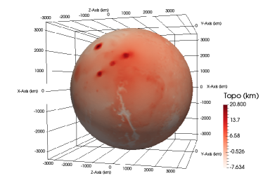
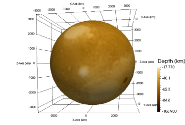
(a) Topography	(b) Crust-mantle interface

Figure 4: Illustration of (a) the topography and (b) the crust-mantle interface of the Mars using MOLA and gravity data zuber1992mars ; smith1999global ; goossens2017evidence .

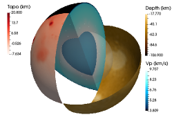
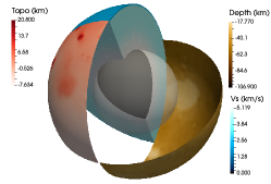
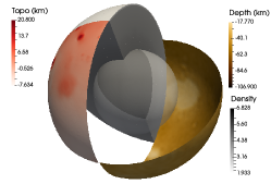
(a) $V_{P}$	(b) $V_{S}$	(c) $\rho^{0}$

Figure 5: Illustration of (a) $V_{P}$, (b) $V_{S}$, and (c) $\rho^{0}$ of our Mars model with a three-dimensional crust shown in Fig. 4.

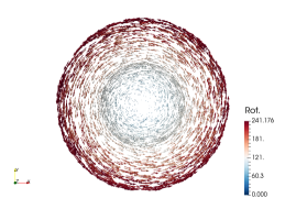
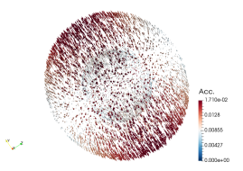
(a) The axial spin mode, $\Omega\times x$ ($m/s$)	(b) Centrifugal acceleration, $-\nabla\psi$ ($m/s^{2}$)

Figure 6: Illustration of (a) the axial spin mode, $\Omega\times x$, and (b) the centrifugal acceleration with $z$ as the rotational axis, $-\nabla\psi$, of the Mars model shown in Fig. 5.

2.2 The basic equations

Given the reference density $\rho^{0}$ and the gravitational constant $G$, we let $\Phi^{0}$ denote the gravitational potential which satisfies,

$$\Delta\Phi^{0}=4\pi G\rho^{0},$$ (1)

and $S(u)$ denote the Eulerian perturbation of the Newtonian potential associated with the displacement $u$,

$$\Delta S(u)=-4\pi G\nabla\cdot(\rho^{0}u).$$ (2)

To include the centrifugal force, we introduce the centrifugal potential

$$\psi(x)=-\frac{1}{2}\left[\Omega^{2}x^{2}-\left(\Omega\cdot x\right)^{2}\right],$$ (3)

where $\Omega\in\mathbb{R}^{3}$ is the angular velocity of rotation. We form the gradient,

$$g^{\prime}=g-\nabla\psi=-\nabla(\Phi^{0}+\psi),$$ (4)

where the reference gravitational field

$$g=-\nabla\Phi^{0}.$$ (5)

The initial stress $T^{0}$ satisfies the mechanical equilibrium given by the static momentum equations,

$$\nabla\cdot T^{0}=-\rho^{0}g^{\prime}.$$ (6)

The elastic-gravitational system of a rotating non-hydrostatic terrestrial planet has the form

$$-\omega^{2}\rho^{0}u+2\operatorname{i}\omega\rho^{0}R_{\Omega}u=\nabla\cdot T^{\mathrm{L1}}-\nabla\cdot(u\cdot\nabla T^{0})-\rho^{\mathrm{E1}}\nabla\Phi^{0}-\rho^{0}\nabla S(u),$$ (7)

where $\omega$ denotes the angular frequency; $R_{\Omega}u=\Omega\,\times\,u$; $\rho^{\mathrm{E1}}=-\nabla\cdot(\rho^{0}u)$ denotes the first-order Eulerian density perturbation and $T^{\mathrm{L1}}=\Upsilon^{T^{0}}\colon\nabla u$ denotes the incremental Lagrangian Cauchy stress. The elasticity tensor, $\Upsilon^{T^{0}}_{ijkl}$, attains the form,

$$\Upsilon^{T^{0}}_{ijkl}=c_{ijkl}+\frac{1}{2}(-T_{ij}^{0}\delta_{kl}+T_{kl}^{0}\delta_{ij}+T_{ik}^{0}\delta_{jl}-T_{jl}^{0}\delta_{ik}+T_{jk}^{0}\delta_{il}-T_{il}^{0}\delta_{jk}),$$

where $c$ denotes the elastic stiffness tensor. In fact, (6) does not determine the entire tensor $T^{0}$. It is common practice to invoke the hydrostatic assumption when $T_{ij}^{0}=-p^{0}\delta_{ij}$; then $\Upsilon^{T^{0}}_{ijkl}$ reduces to $c_{ijkl}$. Under the hydrostatic assumption, we reduce (7) into

$$\omega^{2}\rho^{0}u-2\operatorname{i}\omega\rho^{0}R_{\Omega}u=-\nabla\cdot(c\colon\nabla u)-\nabla(\rho^{0}u\cdot g^{\prime})+\nabla\cdot(\rho^{0}u)g^{\prime}+\rho^{0}\nabla S(u).$$ (8)

The boundary conditions for the system (8) governing a hydrostatic planet are summarized in Table 1.

boundary types	linearized boundary conditions
free surface, $\partial\tilde{X}$	$T^{0}\cdot\nu=0;\quad\nu\cdot T^{\mathrm{L1}}=0$
solid-solid interfaces $\Sigma^{\text{SS}}$	$[\nu\cdot T^{\mathrm{L1}}]^{+}_{-}=0;\quad[T^{0}\cdot\nu]^{+}_{-}=0;\quad[u]^{+}_{-}=0$
fluid-solid interfaces $\Sigma^{\text{FS}}$	$[T^{0}\cdot\nu]^{+}_{-}=0;\quad[u\cdot\nu]^{+}_{-}=0$
& fluid-fluid interfaces $\Sigma^{\text{FF}}$	$[\nu\cdot T^{\mathrm{L1}}]^{+}_{-}=\nu[\nu\cdot T^{\mathrm{L1}}\cdot\nu]^{+}_{-}=0$
all interfaces $\Sigma$ & $\partial\tilde{X}$	$[S(u)]^{+}_{-}=0;\quad[\nabla S(u)\cdot\nu+4\pi G\rho^{0}u\cdot\nu]^{+}_{-}=0$

Table 1: Boundary conditions for a hydrostatic planet (cf. (dahlen1998theoretical, , Table 3.4)).

2.3 The weak formulation

We let $u^{s}$ denote displacement in the solid regions and $u^{f}$ denote displacement in the fluid regions. We treat the solid and fluid parts differently and then deal with $S(u)$ globally. We use $v$ to denote test functions and denote $v^{s}$ and $v^{f}$ for the solid and fluid test displacements, respectively. The mass term from the first and the second term of (8) take the form

$$b_{H}(u,v)=\int_{\Omega^{\text{S}}}(\overline{v}^{s}\cdot u^{s})\rho^{0}\,\mathrm{d}x+\int_{\Omega^{\text{F}}}(\overline{v}^{f}\cdot u^{f})\rho^{0}\,\mathrm{d}x,$$ (9)

and

$$c_{r}(u,v)=\int_{\Omega^{\text{S}}}\overline{v}^{s}\cdot(\Omega\times u^{s})\rho^{0}\,\mathrm{d}x+\int_{\Omega^{\text{F}}}\overline{v}^{f}\cdot(\Omega\times u^{f})\rho^{0}\,\mathrm{d}x,$$ (10)

respectively. We note that the coercivity of the original weak form of the right-hand side of (8), identified as $a_{\text{original}}(u,v)$ in (de2015system, , (3.5)), is not apparent. The early work by Valette valette1989spectre , which is written in French, analyzed this problem in a proper mathematical space while the details can be found in a preprint of a book chapter de2015system . In the work of de2015system , it is revisited and a proper form, $a_{2}(u,v)$, for the weak formulation is introduced. The coercivity of $a_{2}(u,v)$ is established in (de2015system, , Sections 5.2 and 6). The equivalence, that is, $a_{2}(u,v)=a_{\text{original}}(u,v)$ under the boundary conditions (cf. (dahlen1998theoretical, , Table 3.1)), is proven in (de2015system, , Lemma 4.1).

In this work, we will study $a_{2}(u,v)$ under the hydrostatic assumption. The right hand side of (8) can be written in the form

$$a_{2}(u,v)=\int_{\Omega^{\text{S}}}(\nabla\overline{v}^{s})\colon(c\colon\nabla u^{s})\,\mathrm{d}x+\int_{\Sigma^{\text{FS}}}\mathfrak{S}\{(\overline{v}^{s}\cdot g^{\prime})(\nu^{s\rightarrow f}\cdot u^{s})[\rho^{0}]^{f}\}\,\mathrm{d}\Sigma\\ +\int_{\Omega^{\text{S}}}\mathfrak{S}\big{\{}(\nabla\cdot\overline{v}^{s})(g^{\prime}\cdot u^{s})\rho^{0}-u^{s}\cdot(\nabla g^{\prime})\cdot\overline{v}^{s}\rho^{0}-u^{s}\cdot(\nabla\overline{v}^{s})\cdot g^{\prime}\rho^{0}\big{\}}\,\mathrm{d}x\\ +\int_{\Omega^{\text{F}}}\rho^{0}N^{2}\frac{(g^{\prime}\cdot\overline{v}^{f})(g^{\prime}\cdot u^{f})}{\|g^{\prime}\|^{2}}\,\mathrm{d}x+\int_{\Sigma^{\text{FF}}}(g^{\prime}\cdot\nu)(\overline{v}^{f}\cdot\nu)(u^{f}\cdot\nu)[\rho^{0}]^{+}_{-}\,\mathrm{d}\Sigma\\ +\int_{\Omega^{\text{F}}}\kappa(\nabla\cdot\overline{v}^{f}+\rho^{0}\kappa^{-1}g^{\prime}\cdot\overline{v}^{f})(\nabla\cdot u^{f}+\rho^{0}\kappa^{-1}g^{\prime}\cdot u^{f})\,\mathrm{d}x\\ -\frac{1}{4\pi G}\int_{\mathbb{R}^{3}}\nabla S(\overline{v})\cdot\nabla S(u)\,\mathrm{d}x,$$ (11)

where $N^{2}=(\nabla\rho^{0}/\rho^{0}-g^{\prime}\rho^{0}/\kappa)\cdot g^{\prime}$ signifies the square of the Brunt-Väisälä frequency; $\nu^{s\rightarrow f}$ denotes the normal vector at the fluid-solid boundary pointing from the solid to the fluid side; the symmetrization operation $\mathfrak{S}$ is defined as $\mathfrak{S}\{L(u,\overline{v})\}:=\frac{1}{2}(L(u,\overline{v})+L(\overline{v},u))$, for any bilinear form $L(u,v)$. The first integral over $\Omega^{\text{F}}$ is responsible for the inertial or gravity modes, and the second integral over $\Omega^{\text{F}}$ yields the acoustic modes. The integral over $\Sigma^{\text{FF}}$ generates Kelvin modes that occur at boundaries with density jumps. To solve the basic equation (8), we combine (9) with (11) and obtain the system

$$a_{2}(u,v)=\omega^{2}b_{H}(u,v)-\operatorname{i}\omega c_{r}(u,v).$$ (12)

However, it is computationally infeasible to obtain the accurate normal modes from the direct discretization of (12) due to the existence of spurious oscillations kiefling1976fluid . We discuss various approaches in Subsection 2.3.1 and note that the solution needs to be restricted to the space associated with the seismic point spectrum. In Subsections 2.3.2, 2.3.3, 2.3.4 and 2.3.5, we present our scheme to deal with the fluid-solid and fluid surface boundary conditions, fluid regions, solid regions and perturbation of the gravitational potential and field, respectively. In the Subsection 2.4, we introduce the mathematical spaces associated with the seismic point and essential spectra and their separation using a polynomial filtering eigensolver.

2.3.1 Choice of physical variables for fluid regions without rotation

To study planetary normal modes, we include the linear elasticity, compressible fluids, and the fluid-solid and free-surface boundary conditions. Discretization of the standard formulation leads to computational difficulties, since the non-seismic modes from the compressible fluid may pollute the computation of the point spectrum. In this paper, we use a displacement-pressure formulation and later substitute the pressure term using an equivalent formula.

Here, we review different approaches pertaining to the above-mentioned separation of the essential spectrum for non-rotating bodies and then include the rotation. The natural displacement formulation for a non-rotating body will result in a symmetric eigenvalue problem. However, the drawback is the existence of spurious oscillations kiefling1976fluid . Several finite-element methods have been developed for modeling the fluid regions with fluid-solid interaction: a displacement formulation hamdi1978displacement , a pressure formulation zienkiewicz1969coupled ; craggs1971transient , a displacement-pressure formulation wang1997displacement , and a velocity potential formulation everstine1981symmetric ; olson1985analysis . However, the pressure formulation leads to a non-symmetric eigenvalue problem zienkiewicz1969coupled ; craggs1971transient , and the velocity potential formulation everstine1981symmetric ; olson1985analysis leads to a quadratic eigenvalue problem.

In the engineering community, several approaches have been designed to resolve this issue. A penalty method hamdi1978displacement has been applied by imposing an irrotational constraint. However, the study by olson1983study has shown that this penalty method has issues dealing with a solid vibrating in the fluid cavity, which is the case in this paper. A four-node element with a reduced integration using a mass matrix projection technique chen1990vibration has been designed to eliminate the spurious modes. A method using different elements for solid and fluid regions was proposed for two-dimensional bermudez1994finite and three-dimensional cases bermudez1999finite when non-physical spurious modes appear bermudez1995finite . The displacement/pressure formulation wang1997displacement has been developed via introducing mixed elements; still, the fluid-solid coupling needs additional consideration bermudez1994finite ; bermudez1999finite .

Compared with the above-mentioned engineering problems, we encounter a more complicated system (8) with different boundary conditions (cf. Table 1). Due to the presence of the reference gravitational field and the incremental gravitational field, the essential spectrum of the elastic-gravitational system is more complicated than the one of the elastic systems with fluid structures in the engineering problems. In the geophysical community, the pressure formulation komatitsch2002spectral1 ; komatitsch2002spectral2 ; nissen20082 has been commonly used, which is based on replacing the displacement by a scalar potential in the fluid regions. It results in non-symmetric stiffness and mass matrices for a non-rotating body. An alternative approach chaljub2003solving ; chaljub2004spectral ; chaljub2007spectral , using several additional variables to represent the fluid displacement, also leads to a non-symmetric system. To preserve the necessary symmetry and guarantee the correct orthonormality condition for the eigenfunctions or normal modes, we note that the fluid displacement must be kept in the formulation.

2.3.2 Fluid-solid and fluid surface boundary conditions

In this work, to deal with fluid-solid and fluid surface boundary conditions we applied a similar approach wang1997displacement with no any penalty terms by augmenting the system of equations (cf. (11)) and introducing an additional variable, $p$, according to

$$-p\kappa^{-1}=\nabla\cdot u^{f}+\rho^{0}\kappa^{-1}g^{\prime}\cdot u^{f}\ \text{in}\ \Omega^{\text{F}}.$$ (13)

Here, $\kappa$ signifies the compressibility of the fluid. Imposing the fluid-solid boundary condition $\left.\left[\nu^{f\rightarrow s}\cdot u^{f}-\nu^{f\rightarrow s}\cdot u^{s}\right]\right|_{\Sigma^{\text{FS}}}=0$ naturally with the introduction of the additional variable $p$, we obtain the weak form for (13),

$$0 =-\int_{\Omega^{\text{F}}}\overline{v}^{p}p\kappa^{-1}\,\mathrm{d}x+\int_{\Omega^{\text{F}}}\Big{[}(\nabla\overline{v}^{p})\cdot u^{f}-\overline{v}^{p}(g^{\prime}\cdot u^{f})\rho^{0}\kappa^{-1}\Big{]}\,\mathrm{d}x$$

$$-\int_{\Sigma^{\text{FS}}}\overline{v}^{p}(\nu^{f\rightarrow s}\cdot u^{s})\,\mathrm{d}\Sigma-\int_{\partial\tilde{X}^{\text{F}}}\overline{v}^{p}(\nu\cdot u^{f})\,\mathrm{d}\Sigma,$$ (14)

for all the test functions $v^{p}$, where $\nu^{f\rightarrow s}$ denotes the normal vector at the fluid-solid boundary pointing from the fluid to the solid side. Due to the hydrostatic equilibrium, we note that $\nu|_{\partial\tilde{X}^{\text{F}}}$ is parallel to $g^{\prime}$. Using the boundary condition,

$$[\nu\cdot(\kappa\nabla\cdot u^{f})]|_{\partial\tilde{X}^{\text{F}}}=0,$$ (15)

we have the relation

$$(\nu\cdot u^{f})|_{\partial\tilde{X}^{\text{F}}}=-\|g^{\prime}\|^{-1}(g^{\prime}\cdot u^{f})|_{\partial\tilde{X}^{\text{F}}}=(\rho^{0}\|g^{\prime}\|)^{-1}p|_{\partial\tilde{X}^{\text{F}}}.$$ (16)

We using (16) to rewrite (14)

$$0=-\int_{\Omega^{\text{F}}}\overline{v}^{p}p\kappa^{-1}\,\mathrm{d}x+\int_{\Omega^{\text{F}}}\Big{[}(\nabla\overline{v}^{p})\cdot u^{f}-\overline{v}^{p}(g^{\prime}\cdot u^{f})\rho^{0}\kappa^{-1}\Big{]}\,\mathrm{d}x\\ -\int_{\Sigma^{\text{FS}}}\overline{v}^{p}(\nu^{f\rightarrow s}\cdot u^{s})\,\mathrm{d}\Sigma-\int_{\partial\tilde{X}^{\text{F}}}(\rho^{0}\|g^{\prime}\|)^{-1}\overline{v}^{p}p\,\mathrm{d}\Sigma=:c_{g}([u,p],v^{p}).$$ (17)

A short-hand notation $c_{g}([u,p],v^{p})$ in (17) is introduced for simplification. In this work, since we only consider planets with a solid surface, the integral over $\partial\tilde{X}^{\text{F}}$ will be omitted. But it will be needed while including the oceans, or dealing with gas giants, such as Saturn or Jupiter.

2.3.3 Fluid regions

We use (13) in (11) and obtain

$$\int_{\Omega^{\text{F}}}\kappa(\nabla\cdot\overline{v}^{f}+\rho^{0}\kappa^{-1}g^{\prime}\cdot\overline{v}^{f})(\nabla\cdot u^{f}+\rho^{0}\kappa^{-1}g^{\prime}\cdot u^{f})\,\mathrm{d}x\\ =\int_{\Omega^{\text{F}}}[(\overline{v}^{f}\cdot\nabla p)-(\overline{v}^{f}\cdot g^{\prime})p\rho^{0}\kappa^{-1}]\,\mathrm{d}x-\int_{\Sigma^{\text{FS}}}(\overline{v}^{f}\cdot\nu^{f\rightarrow s})p\,\mathrm{d}\Sigma.$$ (18)

Since

$$-\int_{\Sigma^{\text{FS}}}(\overline{v}^{f}\cdot\nu^{f\rightarrow s})p\,\mathrm{d}\Sigma=\int_{\Sigma^{\text{FS}}}(\overline{v}^{s}\cdot\nu^{s\rightarrow f})p\,\mathrm{d}\Sigma,$$ (19)

we include the right-hand side of (19) in the contributions from the solid regions. Thus, we obtain the contributions to $a_{2}(u,v)$ in (11) from the fluid regions,

$$a^{f}_{2}([u,p],v)=\int_{\Omega^{\text{F}}}\rho^{0}N^{2}\frac{(g^{\prime}\cdot\overline{v}^{f})(g^{\prime}\cdot u^{f})}{\|g^{\prime}\|^{2}}\,\mathrm{d}x+\int_{\Omega^{\text{F}}}\overline{v}^{f}\cdot(\nabla p-g^{\prime}p\rho^{0}\kappa^{-1})\,\mathrm{d}x\\ +\int_{\Sigma^{\text{FF}}}(g^{\prime}\cdot\nu)(\overline{v}^{f}\cdot\nu)(u^{f}\cdot\nu)[\rho^{0}]^{+}_{-}\,\mathrm{d}\Sigma.$$ (20)

2.3.4 Solid regions

For the solid regions, we add the right-hand side of (19) to the terms related to the solid regions in (11) and obtain

$$a^{s}_{2}(u,v)=\int_{\Omega^{\text{S}}}(\nabla\overline{v}^{s})\colon(c\colon\nabla u^{s})\,\mathrm{d}x\\ +\int_{\Omega^{\text{S}}}\mathfrak{S}\{(\nabla\cdot\overline{v}^{s})(g^{\prime}\cdot u^{s})\rho^{0}-u^{s}\cdot(\nabla g^{\prime})\cdot\overline{v}^{s}\rho^{0}-u^{s}\cdot(\nabla\overline{v}^{s})\cdot g^{\prime}\rho^{0}\}\,\mathrm{d}x\\ +\int_{\Sigma^{\text{FS}}}\mathfrak{S}\{(\overline{v}^{s}\cdot g^{\prime})(\nu^{s\rightarrow f}\cdot u^{s})[\rho^{0}]^{f}\}\,\mathrm{d}\Sigma+\int_{\Sigma^{\text{FS}}}(\overline{v}^{s}\cdot\nu^{s\rightarrow f})p\,\mathrm{d}\Sigma.$$ (21)

2.3.5 Perturbation of the gravitational potential and field

Here, we discuss the contribution of the perturbation of the gravitational potential $S(u)$. Since the test functions are divided into test functions on solid and fluid regions, we have

$$a_{G}(u,v)=-\frac{1}{4\pi G}\int_{\mathbb{R}^{3}}\nabla S(\overline{v})\cdot\nabla S(u)\,\mathrm{d}x=\\ -\int_{\Omega^{\text{S}}}\nabla\cdot(\rho^{0}\overline{v}^{s})S(u)\,\mathrm{d}x-\int_{\Sigma^{\text{SS}}\cup\partial\tilde{X}^{\text{S}}}(\nu\cdot\overline{v}^{s})S(u)[\rho^{0}]^{+}_{-}\,\mathrm{d}\Sigma\\ -\int_{\Omega^{\text{F}}}\nabla\cdot(\rho^{0}\overline{v}^{f})S(u)\,\mathrm{d}x-\int_{\Sigma^{\text{FF}}\cup\partial\tilde{X}^{\text{F}}}(\nu\cdot\overline{v}^{f})S(u)[\rho^{0}]^{+}_{-}\,\mathrm{d}\Sigma\\ -\int_{\Sigma^{\text{FS}}}\left\{(\nu^{f\rightarrow s}\cdot\overline{v}^{s})S(u)[\rho^{0}]^{s}+(\nu^{s\rightarrow f}\cdot\overline{v}^{f})S(u)[\rho^{0}]^{f}\right\}\,\mathrm{d}\Sigma,$$ (22)

where $[\rho^{0}]^{s}$ denotes the solid density along the fluid-solid boundary. One can set up $S(u)$ as an independent variable and apply the finite-infinite element method to approximate (2), but here we follow a different approach.

Making use of Green’s function (dahlen1998theoretical, , Chapter 3, (3.98)), we have

$$S(u)=G\int_{\tilde{X}}\frac{\nabla^{\prime}\cdot(\rho^{0}(x^{\prime})u(x^{\prime}))}{\|x-x^{\prime}\|}\,\,\mathrm{d}x^{\prime}+G\int_{\Sigma\cup\partial\tilde{X}}\frac{\nu(x^{\prime})\cdot u(x^{\prime})[\rho^{0}(x^{\prime})]^{+}_{-}}{\|x-x^{\prime}\|}\,\,\mathrm{d}\Sigma^{\prime}.$$ (23)

Again, we separate the displacement $u$ into $u^{s}$ and $u^{f}$, and rewrite (23) as

$$S(u)=G\bigg{\{}\int_{\Omega^{\text{S}}}\frac{\nabla^{\prime}\cdot(\rho^{0}(x^{\prime})u^{s}(x^{\prime}))}{\|x-x^{\prime}\|}\,\,\mathrm{d}x^{\prime}+\int_{\Omega^{\text{F}}}\frac{\nabla^{\prime}\cdot(\rho^{0}(x^{\prime})u^{f}(x^{\prime}))}{\|x-x^{\prime}\|}\,\,\mathrm{d}x^{\prime}\\ +\int_{\Sigma^{\text{SS}}\cup\partial\tilde{X}^{\text{S}}}\frac{\nu(x^{\prime})\cdot u^{s}(x^{\prime})[\rho^{0}(x^{\prime})]^{+}_{-}}{\|x-x^{\prime}\|}\,\,\mathrm{d}\Sigma^{\prime}+\int_{\Sigma^{\text{FF}}\cup\partial\tilde{X}^{\text{F}}}\frac{\nu(x^{\prime})\cdot u^{f}(x^{\prime})[\rho^{0}(x^{\prime})]^{+}_{-}}{\|x-x^{\prime}\|}\,\,\mathrm{d}\Sigma^{\prime}\\ +\int_{\Sigma^{\text{FS}}}\frac{[\rho^{0}(x^{\prime})]^{s}\nu^{f\rightarrow s}(x^{\prime})\cdot u^{s}(x^{\prime})+[\rho^{0}(x^{\prime})]^{f}\nu^{s\rightarrow f}(x^{\prime})\cdot u^{f}(x^{\prime})}{\|x-x^{\prime}\|}\,\,\mathrm{d}\Sigma^{\prime}\bigg{\}}.$$ (24)

Although we impose $\nu^{s\rightarrow f}\cdot u^{f}=\nu^{s\rightarrow f}\cdot u^{s}$ along the fluid-solid boundaries, we keep the construction of the incremental gravitational potential $S(u)$ as described in (24). This is to preserve the symmetry of the bilinear form as we substitute (24) into (22).

Since the Green’s solution is known, we apply the FMM to evaluate $S(u)$ for a given displacement $u$ via (24). The utilization of this approach is computationally attractive, but requires that the eigensolver can solve for the interior eigenpairs via matrix-vector multiplications.

2.3.6 Summary

To restrict the system to the computational domain, we can rewrite (11) as

$$a_{2}([u,p],v)=a_{2}^{s}(u,v)+a_{2}^{f}([u,p],v)+a_{G}(u,v).$$ (25)

We obtain the complete formula for the rotating hydrostatic planetary model (9), (10), (25) and (17):

$$\begin{cases}a_{2}([u,p,S(u)],v)&=\omega^{2}b_{H}(u,v)-2\operatorname{i}\omega c_{r}(u,v),\\ c_{g}([u,p],v^{p})&=0.\end{cases}$$ (26)

A matrix representation can be derived from (26). In practice, we replace $p$ in $a_{2}$ by $p(u^{f},u^{s}_{\Sigma^{\text{FS}}})$ via solving the constraint $c_{g}([u,p],v^{p})=0$ in (17) and obtain

$$a_{2}([u,p(u^{f},u^{s}_{\Sigma^{\text{FS}}}),S(u)],v)=\omega^{2}b_{H}(u,v)-2\operatorname{i}\omega c_{r}(u,v).$$ (27)

The corresponding orthonormality condition is that, for an eigenpair $(\omega_{(i)},u^{(i)})$, any other eigenpair $(\omega_{(j)},u^{(j)})$ satisfies

$$b_{H}(u^{(i)},u^{(j)})-2\operatorname{i}(\omega_{(i)}+\omega_{(j)})^{-1}c_{r}(u^{(i)},u^{(j)})=\delta_{ij},$$ (28)

which is consistent with (dahlen1998theoretical, , (4.82)).

2.4 Hilbert space for the elastic-gravitational system

We introduce the space for the displacement field (de2015system, , Definition 5.4)

$$E=\left\{u\in L^{2}(\tilde{X},\rho^{0}\,\mathrm{d}x):\begin{cases}&u^{s}=u|_{\Omega^{\text{S}}}\in H^{1}(\Omega^{\text{S}})\\ &u^{f}=u|_{\Omega^{\text{F}}}\in H(\text{Div},\Omega^{\text{F}},L^{2}(\partial\Omega^{\text{F}}))\\ &[u\cdot\nu]_{-}^{+}=0,\,\text{along}\,\Sigma^{\text{FS}}\end{cases}\right\},$$ (29)

where

$$H(\text{Div},\Omega^{\text{F}},L^{2}(\partial\Omega^{\text{F}}))=\{u^{f}\in L^{2}(\Omega^{\text{F}}):\nabla\cdot u^{f}\in L^{2}(\Omega^{\text{F}}),\,u|_{\partial\Omega^{\text{F}}}\cdot\nu\in L^{2}(\partial\Omega^{\text{F}})\}.$$

$L^{2}(\tilde{X},\rho^{0}\,\mathrm{d}x)$ denotes a weighted $L^{2}$ Hilbert space with

$$L^{2}(\tilde{X},\rho^{0}\,\mathrm{d}x) :=\left\{u:\int_{\tilde{X}}|u|^{2}\rho^{0}\,\mathrm{d}x<\infty\right\};$$

$$\langle u,v\rangle_{L^{2}(\tilde{X},\rho^{0}\,\mathrm{d}x)} :=\int_{\tilde{X}}(u\cdot v)\rho^{0}\,\mathrm{d}x.$$

We write $H=L^{2}(\tilde{X},\rho^{0}\,\mathrm{d}x)$ subject to the constraint $\int_{\tilde{X}}u\rho^{0}\,\mathrm{d}x=0$ removing rigid-body translations; $E$ is densely embedded in $H$ de2019note .

To describe the essential spectrum, we introduce operator $T$ in (valette1989spectre, , Section 4) and de2019note ,

$$Tu^{f}=\rho^{0}[\nabla\cdot u^{f}+\rho^{0}\kappa^{-1}g^{\prime}\cdot u^{f}].$$ (30)

The adjoint, $T^{*}$, of $T$ is given by

$$T^{*}\varphi=-\frac{1}{\rho^{0}}\nabla(\rho^{0}\varphi)+\rho^{0}\kappa^{-1}g^{\prime}\varphi,$$ (31)

where $\varphi$ has the interpretation of potential. A subspace, $H_{2}$, of $H$ associated with the essential spectrum is defined by the constraints

$$u^{s}=0,\ Tu^{f}=0\text{ and }u^{f}\cdot\nu=0\text{ on }\Sigma^{\text{FF}}\cup\Sigma^{\text{FS}}\cup\partial\tilde{X}^{\text{F}}.$$

In fact, $u^{f}$ can be decomposed according to $\text{Ran}(T^{*})\oplus\text{Ker}(T)$, following the decomposition

$$H=H_{1}\oplus H_{2},$$ (32)

where spaces $H_{1}$ and $H_{2}$ are associated with the point and essential spectrum, respectively. The space $H_{2}$ is designed precisely to extract, via projections, the “subseismic” approximations to the full system of governing equations for a contained rotating, compressible, inhomogeneous, self-gravitating fluid. The rigid boundary condition, $u|_{\Omega^{\text{F}}}\cdot\nu=0$ on $\Sigma^{\text{FF}}\cup\partial\tilde{X}^{\text{F}}$, is consistent with a rigid mantle and rigid inner core as $u|_{\Omega^{\text{S}}}=0$.

In fact, $\forall u\in H_{2}$, we obtain $p=0$ and for Cowling approximation, we have

$$a_{2}^{s}(u,v)+a_{2}^{f}(u,v)=\int_{\Omega^{\text{F}}}\rho^{0}N^{2}\frac{(g^{\prime}\cdot\overline{v}^{f})(g^{\prime}\cdot u^{f})}{\|g^{\prime}\|^{2}}\,\mathrm{d}x,$$ (33)

where $a_{2}^{s}$ and $a_{2}^{f}$ are defined in (21) and (20), respectively. For the incremental gravitational potential in (2), we have

$$\Delta S_{H_{2}}(u)=-4\pi G\nabla\cdot(\rho^{0}u^{f})=-4\pi G\left[\rho^{0}N^{2}\frac{(g^{\prime}\cdot u^{f})}{\|g^{\prime}\|^{2}}\right].$$ (34)

Combining (33) and (34), we note that (27) will be reduced to

$$\int_{\Omega^{\text{F}}}\rho^{0}N^{2}\frac{(g^{\prime}\cdot\overline{v}^{f})(g^{\prime}\cdot u^{f})}{\|g^{\prime}\|^{2}}\,\mathrm{d}x-\frac{1}{4\pi G}\int_{\mathbb{R}^{3}}\nabla S_{H_{2}}(\overline{v})\cdot\nabla S_{H_{2}}(u)\,\mathrm{d}x\\ =\omega^{2}b_{H}(u,v)-2\operatorname{i}\omega c_{r}(u,v).$$ (35)

Thus, restricting $\forall u\in H_{2}$, the associated spectrum of (35) will essentially depend on to $N^{2}$ and the rotating rates.

In this work, we solve for the eigenvalues and eigenfunctions of (27) inside a target frequency interval $[f_{1},f_{2}]$, where

$$f_{2}>f_{1}\gg|\Omega|+\left[|\Omega|^{2}+\max\left(0,N^{2}_{\sup}\right)\right]^{1/2},$$ (36)

where $N^{2}_{\sup}$ denotes the supremum of the square of the Brunt-Väisälä frequency. We note that inequality (36) holds true for most planets because the minimal seismic normal mode frequency is typically much larger than the upper bound of the associated spectrum of (35), which is the right hand side of (36). For instance, the maximum of the Brunt-Väisälä frequency of the Earth is around 50 $\mu$Hz and $|\Omega|$ is 7.3 $\mu$Hz while the minimal seismic normal mode frequency is around 0.3 mHz. A well-designed polynomial filter applied with the eigensolver, will have the effect of boosting up the eigenvalues inside the interval $[f_{1},f_{2}]$ while lessening the rest of the spectrum, including the part associated with $H_{2}$.

Remark 1

It is important to understand the need for polynomial filtering in this context. First note that eigensolvers like ARPACK lehoucq1998arpack or subspace iteration, e.g., saad2011numerical , compute eigenvalues of a matrix on one end of the spectrum. After discretizetion, the essential spectrum will give rise to a large number of eigenvalues near zero. Computing the (discrete) eigenvalues in the interval $[f_{1},f_{2}]$ will be numerically challenging unless the small eigenvalues associated with the essential spectrum are eliminated. In numerical linear algebra, this is termed an interior eigenvalue problem in that the target eigenvalues of the discretized problem are located well inside the spectrum. If we use a standard package like ARPACK lehoucq1998arpack we could compute these eigenvalues starting from the smallest ones until we reach the desired interval $[f_{1},f_{2}]$, which would be prohibitive because of the large cluster near zero caused by the essential spectrum. Alternatively, we could compute them from the largest ones down. This would also entail computing a large number of unwanted eigenpairs. Finally, we could also use a shift-and-invert strategy Parlett-book within ARPACK. This requires using a direct solver with a very large matrix and is impractical in our context due to the large memory requirement. The advantage of polynomial filtering is that it eliminates the unwanted eigenvalues and allows the eigensolver to focus on those that are amplified, namely those in $[f_{1},f_{2}]$.

In Section 3, we study the hydrostatic equilibrium of the liquid regions with rotation and derive a proper density distribution. In Section 4, we introduce the mixed FEM to construct the system without the perturbation of the gravitational field. In Section 5, we utilize FMM to compute the gravitational field and the perturbation of the gravitational field and then obtain the complete matrix formula for (27).

3 Hydrostatic equilibrium of the liquid core with rotation

In this section, we discuss the hydrostatic equilibrium with rotation and how it constrains the shape of the boundaries and the density distribution in planets. Rotating fluids have been extensively studied greenspan1968theory ; chandrasekhar2013hydrodynamic ; zhang2017theory . The outer core’s properties have been studied through seismic normal modes since the 1970s gilbert1975application ; dziewonski1975parametrically ; dziewonski1981preliminary , but also with body waves morelli1993body ; kennett1995constraints . Much more recently, an alternative radial outer core model has been proposed using the parametrization of the equation of state for liquid iron alloys at high pressures and temperatures, inferred from eigenfrequency observations irving2018seismically . Furthermore, we mention models for the core of Mars rivoldini2011geodesy ; khan2016single albeit ignoring rotation.

To reach the hydrostatic equilibrium, the prepressure $p^{0}$ satisfies

$$\nabla p^{0}=\rho^{0}g^{\prime},$$ (37)

where $g^{\prime}$ is defined in (4). Well-posedness requires that

$$\nabla\rho^{0}\parallel g^{\prime}\parallel\nabla p^{0}\quad\text{in}\ \Omega^{\text{F}}\quad\text{and}\quad g^{\prime}\parallel\nu\quad\text{along}\ \Sigma^{\text{FS}}\cup\partial\tilde{X}^{\text{F}};$$ (38)

see (de2015system, , Lemma 2.1) for details about the functional properties of $\rho^{0}$, $p^{0}$ and $g^{\prime}$.

The derivation of Clairaut’s equation clairaut1743theorie , and Radau approximation are put in the context of a general scheme imposing (38) in (dahlen1998theoretical, , Chapter 14.1). The bulk parameters of Earth and Mars are listed in Table 2. While the hydrostatic assumption seems to apply to Earth with reasonable accuracy, the derivative of the ellipticity at $r_{e}$, $\dot{\epsilon}(r_{e})$, of Mars appears to be negative, whence this assumption fails to hold dollfus1972new ; bills1978mars .

parameters	$\Omega$ (s-1)	$r_{e}$ (km)	$g_{(r_{e})}$ (m/s2)	$\dot{\epsilon}(r_{e})$	$\epsilon_{(r_{e})}^{\text{hyd}}$	$\epsilon_{(r_{e})}^{\text{obs}}$
Earth	7.2921$e{-5}$	6371.0	9.80	3.05$e{-5}>0$	3.34$e{-3}$	3.35$e{-3}$
Mars	7.0882$e{-5}$	3389.5	3.71	-8.98$e{-5}<0$	N/A	5.89$e{-3}$

Table 2: Bulk parameters of Earth and Mars; $\dot{\epsilon}(r_{e})$ denotes the derivative of $\epsilon$ at $a=r_{e}$, and $\epsilon_{(r_{e})}^{\text{hyd}}$ and $\epsilon_{(r_{e})}^{\text{obs}}$ denote the computed hydrostatic ellipticity and observed ellipticity, respectively.

To construct models of liquid planet interiors, such as Jupiter and Saturn, equations of state and theory of figures are commonly used for calculating a self-consistent shape and gravity field jeans1919problems . We refer to militzer2016understanding for a review on modelling Jupiter’s interior using equations of state and multiple mission data. Since Radau assumptions break down for fast rotating plants (wahltidal, , Fig.3), we refer to hubbard2013concentric ; militzer2019models for constructing Saturn’s interior using the concentric Maclaurin spheroid method to match the Cassini measurements. The condition (38) is satisfied along with other conditions.

4 The Continuous Galerkin mixed finite-element method

In this section, we employ the Continuous Galerkin mixed FEM zienkiewicz2005finite ; bathe2006finite ; hughes2012finite ; brezzi2012mixed ; ern2013theory , for discretizing our system without the perturbation of the gravitational field. We thus obtain a matrix representation for the corresponding weak forms. The incremental gravitational potential will be introduced in the discretization in Subsection 5.2.

4.1 The Continuous Galerkin mixed finite-element approximation

Given a shape regular finite-element partitioning $\mathcal{T}_{h}$ of the domain $\tilde{X}$, we denote an element of the mesh by $K_{k}\in\mathcal{T}_{h}$ and a boundary element by $E_{l}\subset\partial K_{k}$ and have

$$\tilde{X}\approx\bigcup_{k=1}^{N_{K}}K_{k},\quad\Sigma\cup\partial\tilde{X}\approx\bigcup_{l=1}^{N_{E}}E_{l}\subseteq\bigcup_{k=1}^{N_{K}}\partial K_{k},$$

where $N_{K}$ denotes the total number of volume elements and $N_{E}$ denotes the total number of interior and exterior boundary elements. Furthermore, we let $K_{k}^{\text{S}}$ and $K_{k}^{\text{F}}$ be elements in the solid and fluid regions, respectively. Similarly, $E_{l}^{\text{S}}$, $E_{l}^{\text{F}}$ and $E_{l}^{\text{FS}}$ denote boundary elements on the solid $\Sigma^{\text{SS}}\cup\partial\tilde{X}^{\text{S}}$, fluid $\Sigma^{\text{FF}}\cup\partial\tilde{X}^{\text{F}}$ and fluid-solid $\Sigma^{\text{FS}}$ discontinuities, respectively. We have

$$\Omega^{\text{S}} \approx\bigcup_{k=1}^{N_{K}^{\text{S}}}K_{k}^{\text{S}},\quad\Omega^{\text{F}}\approx\bigcup_{k=1}^{N_{K}^{\text{F}}}K_{k}^{\text{F}},$$

$$\Sigma^{\text{FS}} \approx\bigcup_{l=1}^{N_{E}^{\text{FS}}}E_{l}^{\text{FS}},\quad\Sigma^{\text{SS}}\cup\partial\tilde{X}^{\text{S}}\approx\bigcup_{l=1}^{N_{E}^{\text{S}}}E_{l}^{\text{S}},\quad\Sigma^{\text{FF}}\cup\partial\tilde{X}^{\text{F}}\approx\bigcup_{l=1}^{N_{E}^{\text{F}}}E_{l}^{\text{F}}$$

with

$$N_{K}=N_{K}^{\text{S}}+N_{K}^{\text{F}},\quad N_{E}=N_{E}^{\text{S}}+N_{E}^{\text{F}}+N_{E}^{\text{FS}},$$

where $N_{K}^{\text{S}}$ and $N_{K}^{\text{F}}$ denote the total number of volume elements in the solid and fluid regions, respectively, and $N_{E}^{\text{S}}$, $N_{E}^{\text{F}}$ and $N_{E}^{\text{FS}}$ denote the total number of boundary elements on the (interior/exterior) solid, fluid and fluid-solid boundaries, respectively. In the above, $h$ signifies the maximum value of diameters of all the elements.

Since we separate out the fluid and solid regions, we divide the finite-element partitioning accordingly into

$$\mathcal{T}_{h}=\mathcal{T}_{h}^{\text{S}}+\mathcal{T}_{h}^{\text{F}},\quad\Sigma^{\text{FS}}_{h}=\mathcal{T}_{h}^{\text{S}}\cap\mathcal{T}_{h}^{\text{F}},$$

where $\mathcal{T}_{h}^{\text{S}}$, $\mathcal{T}_{h}^{\text{F}}$ and $\Sigma^{\text{FS}}_{h}$ denote the partitioning of the domains $\Omega^{\text{S}}$, $\Omega^{\text{F}}$ and boundary $\Sigma^{\text{FS}}$, respectively. We then introduce $E_{h}$ as the finite-element space corresponding with the displacement space $E$ in (29),

$$E_{h}=\left\{u_{h}:\begin{cases}&u^{s}_{h}\in\mathbf{V}_{h}^{s}:=\left\{v^{s}_{h}\in H^{1}(\Omega^{\text{S}}):v^{s}_{h}|_{K}\in\mathcal{P}_{p^{s}}(K),\ K\in\mathcal{T}_{h}^{\text{S}}\right\},\\ &u^{f}_{h}\in\mathbf{V}_{h}^{f}:=\Big{\{}v^{f}_{h}\in H(\text{Div},\Omega^{\text{F}},L^{2}(\partial\Omega^{\text{F}}):\\ &\quad\quad\quad\quad\quad\quad\quad\quad\quad\quad\quad\quad v^{f}_{h}|_{K}\in\mathcal{P}_{p^{f}}(K),\ K\in\mathcal{T}_{h}^{\text{F}}\Big{\}},\\ &\displaystyle\int_{E^{{\text{FS}}}}[u_{h}\cdot\nu]_{-}^{+}v^{p}_{h}\,\mathrm{d}\Sigma=0\ \text{for all}\ E^{{\text{FS}}}\subset\Sigma^{\text{FS}}_{h},\end{cases}\right\}$$ (39)

and $\mathbf{V}_{h}^{p}$ as the finite-element space for $p$,

$$\mathbf{V}_{h}^{p}:=\left\{v^{p}_{h}\in H^{1}(\Omega^{\text{F}}):v^{p}_{h}|_{K}\in\mathcal{P}_{p^{p}}(K),\ K\in\mathcal{T}_{h}^{\text{F}}\right\}.$$

Here, $\mathcal{P}_{p^{s}}(K)$ and $\mathcal{P}_{p^{f}}(K)$ are the spaces of polynomials of degrees $p^{s}$ and $p^{f}$, respectively; $\mathcal{P}_{p^{p}}(K)$ is the space of polynomials of degree $p^{p}$. Though the $u_{h}^{f}$ is discretized as $u_{h}^{f}\in H^{1}(\Omega^{\text{F}})$, the constraint equation (13) restricts $u_{h}^{f}\in H(\text{Div},\Omega^{\text{F}},L^{2}(\partial\Omega^{\text{F}})$. By the Galerkin method, the finite-element solutions, $u_{h}$, and the test functions, $v_{h}$, both lie in $E_{h}$ and $\mathbf{V}_{h}^{p}$. We note that the polynomial degree $p^{p}$ does not need to be equal to $p^{f}$.

We apply non-conforming finite elements across the fluid-solid boundaries. The fluid-solid transmission condition in the definition of $E$ has been replaced by the condition $\int_{E^{{\text{FS}}}}[u_{h}\cdot\nu]_{-}^{+}v^{p}_{h}\,\mathrm{d}\Sigma=0$ in the definition of $E_{h}$. The fluid-solid transmission condition holds in the form of a boundary integration. For low-degree polyomials we show, in the next subsection, that these conditions are compatible through our formulation. Such a compatibility was analyzed and discussed by bermudez1994finite ; bermudez1995finite ; brezzi2012mixed . Several numerical studies kiefling1976fluid ; zienkiewicz1978fluid ; olson1985analysis ; chen1990vibration ; bermudez1999finite have been performed using similar non-conforming schemes along the fluid-solid boundaries. For the general theory and analysis of the mixed FEM, we refer to brezzi2012mixed .

4.2 Matrix formulae

operations	physical meanings	corresponding formulae
		$\displaystyle\int_{\Omega^{\text{S}}}\nabla\overline{v}^{s}_{h}:(c:\nabla u^{s}_{h})\,\mathrm{d}x$
		$\displaystyle+\int_{\Sigma^{\text{FS}}}\mathfrak{S}\Big{\{}(\overline{v}^{s}_{h}\cdot g^{\prime})(\nu^{s\rightarrow f}\cdot u^{s}_{h})[\rho^{0}]^{f}\Big{\}}\,\mathrm{d}\Sigma$
$\displaystyle(\tilde{v}^{s})^{\mathsf{H}}A_{sg}\tilde{u}^{s}$	solid stiffness matrix with gravity	$\displaystyle+\int_{\Omega^{\text{S}}}\mathfrak{S}\Big{\{}(\nabla\cdot\overline{v}^{s}_{h})(g^{\prime}\cdot u^{s}_{h})\rho^{0}$
		$\displaystyle-u^{s}_{h}\cdot(\nabla g^{\prime})\cdot\overline{v}^{s}_{h}\rho^{0}-u^{s}_{h}\cdot(\nabla\overline{v}^{s}_{h})\cdot g^{\prime}\rho^{0}\Big{\}}\,\mathrm{d}x$
		$\displaystyle\int_{\Omega^{\text{F}}}\rho^{0}N^{2}\frac{(g^{\prime}\cdot\overline{v}^{f}_{h})(g^{\prime}\cdot u^{f}_{h})}{\|g^{\prime}\|^{2}}\,\mathrm{d}x$
$\displaystyle(\tilde{v}^{f})^{\mathsf{H}}A_{f}\tilde{u}^{f}$	buoyancy term	$\displaystyle+\int_{\Sigma^{\text{FF}}}(g^{\prime}\cdot\nu)(\overline{v}^{f}_{h}\cdot\nu)(u^{f}_{h}\cdot\nu)[\rho^{0}]^{+}_{-}\,\mathrm{d}\Sigma$
$\displaystyle(\tilde{v}^{p})^{\mathsf{H}}A_{p}\tilde{p}$	fluid potential	$\displaystyle-\int_{\Omega^{\text{F}}}\overline{v}^{p}_{h}p_{h}\kappa^{-1}\,\mathrm{d}x-\int_{\Sigma^{\text{FS}}}\overline{v}^{p}(\nu^{f\rightarrow s}\cdot u^{s})\,\mathrm{d}\Sigma$
$\displaystyle(\tilde{v}^{f})^{\mathsf{H}}A_{\text{dg}}\tilde{p}$	fluid stiffness matrix with gravity	$\displaystyle\int_{\Omega^{\text{F}}}\left[\overline{v}^{f}_{h}\cdot(\nabla p_{h})-(\overline{v}^{f}_{h}\cdot g^{\prime})p_{h}\rho^{0}\kappa^{-1}\right]\,\mathrm{d}x$
$\displaystyle(\tilde{v}^{p})^{\mathsf{H}}A_{\text{dg}}^{\mathsf{T}}\tilde{u}^{f}$	constraint with gravity	$\displaystyle\int_{\Omega^{\text{F}}}\Big{[}(\nabla\overline{v}^{p}_{h})\cdot u^{f}_{h}-\overline{v}^{p}_{h}(g^{\prime}\cdot u^{f}_{h})\rho^{0}\kappa^{-1}\Big{]}\,\mathrm{d}x$
$\displaystyle(\tilde{v}^{s})^{\mathsf{H}}E_{\text{FS}}\tilde{p}$	fluid-solid boundary condition	$\displaystyle\int_{\Sigma^{\text{FS}}}(\overline{v}^{s}_{h}\cdot\nu^{s\rightarrow f})p_{h}\,\mathrm{d}\Sigma$
$\displaystyle(\tilde{v}^{p})^{\mathsf{H}}E_{\text{FS}}^{\mathsf{T}}\tilde{u}^{f}$	fluid-solid boundary condition	$\displaystyle\int_{\Sigma^{\text{FS}}}-\overline{v}^{p}_{h}(\nu^{f\rightarrow s}\cdot u^{s}_{h})\,\mathrm{d}\Sigma$
$\displaystyle(\tilde{v}^{s})^{\mathsf{H}}R_{s}\tilde{u}^{s}$	Coriolis force in $\Omega^{\text{S}}$	$\displaystyle\int_{\Omega^{\text{S}}}\overline{v}^{s}_{h}\cdot\big{(}\Omega\times u^{s}_{h}\big{)}\rho^{0}\,\mathrm{d}x$
$\displaystyle(\tilde{v}^{f})^{\mathsf{H}}R_{f}\tilde{u}^{f}$	Coriolis force in $\Omega^{\text{F}}$	$\displaystyle\int_{\Omega^{\text{F}}}\overline{v}^{f}_{h}\cdot\big{(}\Omega\times u^{f}_{h}\big{)}\rho^{0}\,\mathrm{d}x$
$\displaystyle(\tilde{v}^{s})^{\mathsf{H}}M_{s}\tilde{u}^{s}$	solid mass matrix	$\displaystyle\int_{\Omega^{\text{S}}}(\overline{v}^{s}_{h}\cdot u^{s}_{h})\rho^{0}\,\mathrm{d}x$
$\displaystyle(\tilde{v}^{f})^{\mathsf{H}}M_{f}\tilde{u}^{f}$	fluid mass matrix	$\displaystyle\int_{\Omega^{\text{F}}}(\overline{v}^{f}_{h}\cdot u^{f}_{h})\rho^{0}\,\mathrm{d}x$

Table 3: Implicit definition of the matrices. In the above, $\int_{\Omega^{\text{S}}}=\sum_{k=1}^{N^{\text{S}}_{K}}\int_{K_{k}^{\text{S}}}$, $\int_{\Omega^{\text{F}}}=\sum_{k=1}^{N^{\text{F}}_{K}}\int_{K_{k}^{\text{F}}}$ and $\int_{\Sigma^{\text{FS}}}=\sum_{l=1}^{N^{\text{FS}}_{E}}\int_{E_{l}^{\text{FS}}}$.

We introduce nodal-based Lagrange polynomials, $\{\ell^{s}_{i}\}$, $\{\ell^{f}_{i}\}$, $\{\ell^{p}_{i}\}$, on the respective volume elements $K\in\mathcal{T}^{\text{S}}_{h}$, $\mathcal{T}^{\text{F}}_{h}$. We set $N_{p^{s}}=(p^{s}+1)(p^{s}+2)(p^{s}+3)/6$, where $N_{p^{s}}$ is the number of nodes on a tetrahedron for the $p^{s}$-th order polynomial approximation. We have similar expressions for $N_{p^{f}}$ and $N_{p^{p}}$. We write

$$(u_{h}^{s})_{j}(x) =\sum_{i=1}^{N_{p^{s}}}(u_{h}^{s})_{j}(x_{i})\ell^{s}_{i}(x),$$ (40)

$$(u_{h}^{f})_{j}(x) =\sum_{i=1}^{N_{p^{f}}}(u_{h}^{f})_{j}(x_{i})\ell^{f}_{i}(x),$$ (41)

$$p_{h}(x) =\sum_{i=1}^{N_{p^{p}}}p(x_{i})\ell^{p}_{i}(x),$$ (42)

for $x\in K$; similar representations hold for $v^{s}_{h}$, $v^{f}_{h}$, $v^{p}_{h}$, respectively. We collect the values of $u^{s}_{h}$, $u^{f}_{h}$, $p_{h}$ and $v^{s}_{h}$, $v^{f}_{h}$, $v^{p}_{h}$ at all the nodes, $\{x_{i}\}$, in the vectors $\tilde{u}^{s}$, $\tilde{u}^{f}$, $\tilde{p}$ and $\tilde{v}^{s}$, $\tilde{v}^{f}$, $\tilde{v}^{p}$, respectively. We can then construct the corresponding submatrices, $A_{sg}$, $A_{f}$, $A_{p}$, $A_{\text{dg}}$, $A_{\text{dg}}^{\mathsf{T}}$, $E_{\text{FS}}$, $E_{\text{FS}}^{\mathsf{T}}$, $R_{s}$, $R_{f}$, $M_{s}$ and $M_{f}$, see Table 3, in a standard way summarized in Appendix A.

5 Self-gravitation as an N-body problem

Self-gravitation can be treated as the solution of an N-body problem. We discretize the entire planet into many elements and consider them as individual bodies. The gravitational potential and field are then computed through the interaction between these bodies. We note that FMM is an ideal candidate for solving an N-body problem. FMM reduces the complexity of the N-body problem from $O(N^{2})$ to $O(N\log N)$ or even $O(N)$ greengard1987fast . We apply the FMM greengard1997new ; gimbutas2011fmmlib3d to calculate the reference gravitational potential in Subsection 6.1. We employ ExaFMM yokota2013fmm , a massively parallel N-body problem solver, to solve for the perturbation of the gravitational potential.

5.1 Reference gravitational potential and gravitational field

For calculating the reference gravitational potential and field, we need to evaluate two integrals (dahlen1998theoretical, , (3.2) and (3.3)). The N-body problem of gravitation requires the evaluation of

$$\Phi^{0}(\mathbf{x}_{i})=-G\sum_{k=1}^{N_{K}}\frac{1}{\|\mathbf{x}_{i}-\mathbf{r}_{k}\|}\int_{K_{k}}\rho_{k}^{0}\,\mathrm{d}x$$ (43)

for the potential in (1) and

$$g(\mathbf{x}_{i})=-G\sum_{k=1}^{N_{K}}\frac{\mathbf{x}_{i}-\mathbf{r}_{k}}{\|\mathbf{x}_{i}-\mathbf{r}_{k}\|^{3/2}}\int_{K_{k}}\rho_{k}^{0}\,\mathrm{d}x$$ (44)

for the field in (5). Here, $\mathbf{x}_{i}$ denotes the location of the target vertex and $\mathbf{r}_{k}$ denotes the barycenter of element $K_{k}$.

5.2 Incremental gravitational potential

For calculating the incremental gravitational potential, we need to evaluate (23) containing both the volume and boundary integral terms. Given the finite-element partitioning, $\mathcal{T}_{h}$, we approximate $S(u_{h})$ in (2) via

$$S_{k_{2}}(u_{h})=G\int_{K_{k_{2}}}\frac{\nabla\cdot(\rho_{k_{2}}^{0}(x)u_{h}(x))}{\|\mathbf{r}_{k_{2}}-x\|}\,\mathrm{d}x+\sum\limits_{\begin{subarray}{c}k_{1}=1\\ k_{1}\neq k_{2}\end{subarray}}^{N_{K}}\frac{G}{\|\mathbf{r}_{k_{2}}-\mathbf{r}_{k_{1}}\|}\int_{K_{k_{1}}}\nabla\cdot(\rho_{k_{1}}^{0}u_{h})\,\mathrm{d}x\\ +\sum_{l_{1}=1}^{N_{E}}\frac{G}{\|\mathbf{r}_{k_{2}}-\mathbf{r}_{l_{1}}\|}\int_{E_{l_{1}}}(\nu\cdot u_{h})[\rho_{l_{1}}^{0}]^{+}_{-}\,\mathrm{d}\Sigma$$ (45)

and

$$S_{l_{2}}(u_{h})=G\int_{E_{l_{2}}}\frac{\nu(x)\cdot u_{h}(x)[\rho_{l_{2}}^{0}(x)]^{+}_{-}}{\|\mathbf{r}_{l_{2}}-x\|}\,\mathrm{d}\Sigma+\sum_{\begin{subarray}{c}l_{1}=1\\ l_{1}\neq l_{2}\end{subarray}}^{N_{E}}\frac{G}{\|\mathbf{r}_{l_{2}}-\mathbf{r}_{l_{1}}\|}\int_{E_{l_{1}}}(\nu\cdot u_{h})[\rho_{l_{1}}^{0}]^{+}_{-}\,\mathrm{d}\Sigma\\ +\sum\limits_{\begin{subarray}{c}k_{1}=1\end{subarray}}^{N_{K}}\frac{G}{\|\mathbf{r}_{l_{2}}-\mathbf{r}_{k_{1}}\|}\int_{K_{k_{1}}}\nabla\cdot(\rho_{k_{1}}^{0}u_{h})\,\mathrm{d}x,$$ (46)

where $k_{1}$ and $k_{2}$ label the elements $K_{k_{1}}$ and $K_{k_{2}}$, $S_{k_{2}}(u_{h})$ is the incremental gravitational potential $S(u_{h})$ at the barycenter of $K_{k_{2}}$, $l_{1}$ and $l_{2}$ label the triangular elements $E_{l_{1}}$ and $E_{l_{2}}$, $\mathbf{r}_{l_{1}}$ and $\mathbf{r}_{l_{2}}$ denote the barycenters of $E_{l_{1}}$ and $E_{l_{2}}$. The first terms in (45) and (46) indicate the self-contribution.

Since the variation of $\nabla\cdot(\rho_{k_{2}}^{0}(x)u_{h}(x))$ is small on element $K_{k_{2}}$, we simplify the first term in (45) according to

$$G\int_{K_{k_{2}}}\frac{\nabla\cdot(\rho_{k_{2}}^{0}(x)u_{h}(x))}{\|\mathbf{r}_{k_{2}}-x\|}\,\mathrm{d}x\simeq G\frac{\int_{K_{k_{2}}}\nabla\cdot(\rho_{k_{2}}^{0}u_{h})\,\mathrm{d}x}{|K_{k_{2}}|}\int_{K_{k_{2}}}\frac{1}{\|\mathbf{r}_{k_{2}}-x\|}\,\mathrm{d}x,$$

where $|K_{k_{2}}|$ denotes the volume of element $K_{k_{2}}$. We let

$$\frac{1}{R_{k_{2}}}=\frac{1}{|K_{k_{2}}|}\int_{K_{k_{2}}}\frac{1}{\|\mathbf{r}_{k_{2}}-x\|}\,\mathrm{d}x,$$

and obtain

$$G\int_{K_{k_{2}}}\frac{\nabla\cdot(\rho_{k_{2}}^{0}(x)u_{h}(x))}{\|\mathbf{r}_{k_{2}}-x\|}\,\mathrm{d}x\simeq\frac{G}{R_{k_{2}}}\int_{K_{k_{2}}}\nabla\cdot(\rho_{k_{2}}^{0}u_{h})\,\mathrm{d}x.$$ (47)

Similarly, we simplify the first term in (46) according to

$$G\int_{E_{l_{2}}}\frac{\nu(x)\cdot u_{h}(x)[\rho_{l_{2}}^{0}(x)]^{+}_{-}}{\|\mathbf{r}_{l_{2}}-x\|}\,\mathrm{d}\Sigma\simeq\frac{G}{R_{l_{2}}}\int_{E_{l_{2}}}(\nu\cdot u_{h})[\rho_{l_{1}}^{0}]^{+}_{-}\,\mathrm{d}\Sigma,$$ (48)

with

$$\frac{1}{R_{l_{2}}}=\frac{1}{|E_{l_{2}}|}\int_{E_{l_{2}}}\frac{1}{\|\mathbf{r}_{l_{2}}-x\|}\,\mathrm{d}\Sigma,$$

where $|E_{l_{2}}|$ denotes the area of the boundary element $E_{l_{2}}$. Note that $R_{k_{2}}$ in (47) and $R_{l_{2}}$ in (48) can be precomputed on each element and surface. The second and third terms in (45) and (46) may be evaluated via FMM.

operations	physical meanings	corresponding formulae
		$\displaystyle\int_{\Omega^{\text{S}}}\nabla\cdot(\rho^{0}u^{s}_{h})\,\mathrm{d}x,$
		$\displaystyle\int_{\Sigma^{\text{FS}}}(\nu^{f\rightarrow s}\cdot u^{s}_{h})\left[\rho^{0}\right]^{s}\,\mathrm{d}x,$
$\displaystyle C_{s}\tilde{u}^{s}$	N bodies in $\overline{\Omega^{\text{S}}}$	$\displaystyle\int_{\Sigma^{\text{SS}\cup\partial\tilde{X}^{\text{S}}}}(\nu\cdot u^{s}_{h})\left[\rho^{0}\right]^{+}_{-}\,\mathrm{d}x$
		$\displaystyle\int_{\Omega^{\text{F}}}\nabla\cdot(\rho^{0}u^{f}_{h})\,\mathrm{d}x,$
		$\displaystyle\int_{\Sigma^{\text{FS}}}(\nu^{s\rightarrow f}\cdot u^{f}_{h})\left[\rho^{0}\right]^{f}\,\mathrm{d}x,$
$\displaystyle C_{f}\tilde{u}^{f}$	N bodies in $\overline{\Omega^{\text{F}}}$	$\displaystyle\int_{\Sigma^{\text{FF}\cup\partial\tilde{X}^{\text{F}}}}(\nu\cdot u^{f}_{h})\left[\rho^{0}\right]^{+}_{-}\,\mathrm{d}x$
		$\displaystyle G\int_{\tilde{X}}\frac{\nabla^{\prime}\cdot(\rho^{0}(x^{\prime})u_{h}(x^{\prime}))}{\|x-x^{\prime}\|}\,\,\mathrm{d}x^{\prime}$
$\displaystyle S(C\tilde{u})$	solution for Poisson’s equation	$\displaystyle+G\int_{\Sigma\cup\partial\tilde{X}}\frac{\nu(x^{\prime})\cdot u_{h}(x^{\prime})[\rho^{0}(x^{\prime})]^{+}_{-}}{\|x-x^{\prime}\|}\,\,\mathrm{d}x^{\prime}$
		$\displaystyle\int_{\Omega^{\text{S}}}\nabla\cdot(\rho^{0}\overline{v}^{s}_{h})S(u_{h})\,\mathrm{d}x$
	incremental gravitational field	$\displaystyle+\int_{\Sigma^{\text{FS}}}(\overline{v}^{s}_{h}\cdot\nu^{f\rightarrow s})S(u_{h})[\rho^{0}]^{s}\,\mathrm{d}x$
$\displaystyle(\tilde{v}^{s})^{\mathsf{H}}C_{s}^{\mathsf{T}}(SC\tilde{u})$	in $\overline{\Omega^{\text{S}}}$	$\displaystyle+\int_{\Sigma^{\text{SS}}\cup\partial\tilde{X}^{\text{S}}}(\overline{v}^{s}_{h}\cdot\nu)S(u_{h})[\rho^{0}]^{+}_{-}\,\mathrm{d}x$
		$\displaystyle\int_{\Omega^{\text{F}}}\nabla\cdot(\rho^{0}\overline{v}^{f}_{h})S(u_{h})\,\mathrm{d}x$
	incremental gravitational field	$\displaystyle+\int_{\Sigma^{\text{FS}}}(\overline{v}^{f}_{h}\cdot\nu^{s\rightarrow f})S(u_{h})[\rho^{0}]^{f}\,\mathrm{d}x$
$\displaystyle(\tilde{v}^{s})^{\mathsf{H}}C_{f}^{\mathsf{T}}(SC\tilde{u})$	in $\overline{\Omega^{\text{F}}}$	$\displaystyle+\int_{\Sigma^{\text{FF}}\cup\partial\tilde{X}^{\text{F}}}(\overline{v}^{f}_{h}\cdot\nu)S(u_{h})[\rho^{0}]^{+}_{-}\,\mathrm{d}x$

Table 4: Implicit definition of the submatrices for perturbation to the gravitational potential.

5.2.1 Solid planets

For solid planets, we substitute (47) and (48) into (45) and (46), respectively. To evaluate (22) for a solid planet, we need to compute

$$a_{G}^{s}(u^{s}_{h},v^{s}_{h})=-\sum\limits_{k_{2}=1}^{N_{K}}\int_{K_{k_{2}}^{\text{S}}}\left(\nabla\cdot(\rho^{0}_{k_{2}}\overline{v}^{s}_{h})\right)S_{k_{2}}(u^{s}_{h})\,\mathrm{d}x\\ -\sum\limits_{l_{2}=1}^{N_{E}}\int_{E_{l_{2}}^{\text{S}}}(\nu\cdot\overline{v}^{s}_{h})S_{l_{2}}(u^{s}_{h})[\rho^{0}_{l_{2}}]^{+}_{-}\,\mathrm{d}\Sigma.$$ (49)

We add (49) into the matrix representation and obtain

$$\omega^{2}M_{s}\tilde{u}^{s}-2\operatorname{i}\omega R_{s}\tilde{u}^{s}-\big{(}A_{sg}-C_{s}^{\mathsf{T}}S_{s}C_{s}\big{)}\tilde{u}^{s}=0,$$ (50)

where $C_{s}\tilde{u}^{s}$ evaluates $S_{k_{2}}(u^{s}_{h})$ and $S_{l_{2}}(u^{s}_{h})$, $S_{s}$ solves the N-body problem for the solid planet, and $C_{s}^{\mathsf{T}}S_{s}C_{s}\tilde{u}^{s}$ evaluates (49); the submatrix $A_{sg}$ and its corresponding weak formula is shown in Table 3, and the submatrices $C_{s},C_{s}^{\mathsf{T}},S$ and their corresponding weak formulae are shown in Table 4. Here, of course, $A_{sg}$, $C_{s}$ and $C_{s}^{\mathsf{T}}$ do not include terms related the fluid-solid boundaries $\Sigma^{\text{FS}}$.

5.2.2 Planets with fluid regions

For a planet with fluid regions, we also substitute (47) and (48) into (45) and (46), respectively. To ensure the Hermitian property of the system, we carefully treat the fluid-solid boundary terms and evaluate the incremental gravitational potential $S(u_{h})$ via (24) and obtain the volume integral contributions

$$S_{k_{2}}(u_{h})=\frac{G}{R_{k_{2}}}\int_{K_{k_{2}}}\nabla\cdot(\rho_{k_{2}}^{0}u_{h})\,\mathrm{d}x\\ +\sum\limits_{\begin{subarray}{c}k_{1}=1\\ k_{1}\neq k_{2}\end{subarray}}^{N_{K}^{\text{S}}}\frac{G}{\|\mathbf{r}_{k_{2}}-\mathbf{r}_{k_{1}}\|}\int_{K_{k_{1}}^{\text{S}}}\nabla\cdot(\rho_{k_{1}}^{0}u^{s}_{h})\,\mathrm{d}x+\sum_{l_{1}=1}^{N_{E}^{\text{S}}}\frac{G}{\|\mathbf{r}_{k_{2}}-\mathbf{r}_{l_{1}}\|}\int_{E_{l_{1}}^{\text{S}}}(\nu\cdot u^{s}_{h})[\rho_{l_{1}}^{0}]^{+}_{-}\,\mathrm{d}\Sigma\\ +\sum\limits_{\begin{subarray}{c}k_{1}=1\\ k_{2}\neq k_{2}\end{subarray}}^{N_{K}^{\text{F}}}\frac{G}{\|\mathbf{r}_{k_{2}}-\mathbf{r}_{k_{1}}\|}\int_{K_{k_{1}}^{\text{F}}}\nabla\cdot(\rho_{k_{1}}^{0}u^{f}_{h})\,\mathrm{d}x+\sum_{l_{1}=1}^{N_{E}^{\text{F}}}\frac{G}{\|\mathbf{r}_{k_{2}}-\mathbf{r}_{l_{1}}\|}\int_{E_{l_{1}}^{\text{F}}}(\nu\cdot u^{f}_{h})[\rho_{l_{1}}^{0}]^{+}_{-}\,\mathrm{d}\Sigma\\ +\sum_{l_{1}=1}^{N_{E}^{\text{FS}}}\frac{G}{\|\mathbf{r}_{k_{2}}-\mathbf{r}_{l_{1}}\|}\int_{E_{l_{1}}^{\text{FS}}}\left\{(\nu^{f\rightarrow s}\cdot u^{s}_{h})[\rho_{l_{1}}^{0}]^{s}+(\nu^{s\rightarrow f}\cdot u^{f}_{h})[\rho_{l_{1}}^{0}]^{f}\right\}\,\mathrm{d}\Sigma,$$ (51)

and boundary integral contributions

$$S_{l_{2}}(u_{h})=\frac{G}{R_{l_{2}}}\int_{E_{l_{2}}}(\nu\cdot u_{h})[\rho_{l_{2}}^{0}]^{+}_{-}\,\mathrm{d}\Sigma\\ +\sum\limits_{\begin{subarray}{c}k_{1}=1\end{subarray}}^{N_{K}^{\text{S}}}\frac{G}{\|\mathbf{r}_{l_{2}}-\mathbf{r}_{k_{1}}\|}\int_{K_{k_{1}}^{\text{S}}}\nabla\cdot(\rho_{k_{1}}^{0}u^{s}_{h})\,\mathrm{d}x+\sum_{\begin{subarray}{c}l_{1}=1\\ l_{1}\neq l_{2}\end{subarray}}^{N_{E}^{\text{S}}}\frac{G}{\|\mathbf{r}_{l_{2}}-\mathbf{r}_{l_{1}}\|}\int_{E_{l_{1}}^{\text{S}}}(\nu\cdot u^{s}_{h})[\rho_{l_{1}}^{0}]^{+}_{-}\,\mathrm{d}\Sigma\\ +\sum\limits_{\begin{subarray}{c}k_{1}=1\end{subarray}}^{N_{K}^{\text{F}}}\frac{G}{\|\mathbf{r}_{l_{2}}-\mathbf{r}_{k_{1}}\|}\int_{K_{k_{1}}^{\text{F}}}\nabla\cdot(\rho_{k_{1}}^{0}u^{f}_{h})\,\mathrm{d}x+\sum_{\begin{subarray}{c}l_{1}=1\\ l_{1}\neq l_{2}\end{subarray}}^{N_{E}^{\text{F}}}\frac{G}{\|\mathbf{r}_{l_{2}}-\mathbf{r}_{l_{1}}\|}\int_{E_{l_{1}}^{\text{F}}}(\nu\cdot u^{s}_{h})[\rho_{l_{1}}^{0}]^{+}_{-}\,\mathrm{d}\Sigma\\ +\sum_{l_{1}=1}^{N_{E}^{\text{FS}}}\frac{G}{\|\mathbf{r}_{l_{2}}-\mathbf{r}_{l_{1}}\|}\int_{E_{l_{1}}^{\text{FS}}}\left\{(\nu^{f\rightarrow s}\cdot u^{s}_{h})[\rho_{l_{1}}^{0}]^{s}+(\nu^{s\rightarrow f}\cdot u^{f}_{h})[\rho_{l_{1}}^{0}]^{f}\right\}\,\mathrm{d}\Sigma.$$ (52)

With (51) and (52), we have the full solution for the incremental gravitational potential. To evaluate (22) for a planet with fluid regions, we need to compute

$$a_{G}(u_{h},v_{h})=\\ -\sum\limits_{k_{2}=1}^{N_{K}^{\text{S}}}\int_{K_{k_{2}}^{\text{S}}}\left(\nabla\cdot(\rho^{0}_{k_{2}}\overline{v}^{s}_{h})\right)S_{k_{2}}(u_{h})\,\mathrm{d}x-\sum\limits_{l_{2}=1}^{N_{E}^{\text{S}}}\int_{E_{l_{2}}^{\text{S}}}(\nu\cdot\overline{v}^{s}_{h})S_{l_{2}}(u_{h})[\rho^{0}_{l_{2}}]^{+}_{-}\,\mathrm{d}\Sigma\\ -\sum\limits_{k_{2}=1}^{N_{K}^{\text{F}}}\int_{K_{k_{2}}^{\text{F}}}\left(\nabla\cdot(\rho^{0}_{k_{2}}\overline{v}^{f}_{h})\right)S_{k_{2}}(u_{h})\,\mathrm{d}x-\sum\limits_{l_{2}=1}^{N_{E}^{\text{F}}}\int_{E_{l_{2}}^{\text{F}}}(\nu\cdot\overline{v}^{f}_{h})S_{l_{2}}(u_{h})[\rho^{0}_{l_{2}}]^{+}_{-}\,\mathrm{d}\Sigma\\ -\sum_{l_{2}=1}^{N_{E}^{\text{FS}}}\int_{E_{l_{2}}^{\text{FS}}}\left\{(\nu^{f\rightarrow s}\cdot\overline{v}^{s}_{h})S_{l_{2}}(u_{h})[\rho^{0}_{l_{2}}]^{s}+(\nu^{s\rightarrow f}\cdot\overline{v}^{f}_{h})S_{l_{2}}(u_{h})[\rho^{0}_{l_{2}}]^{f}\right\}\,\mathrm{d}\Sigma.$$ (53)

We derive the matrix representation with (53) and obtain

$$\omega^{2}M\tilde{u}-2\operatorname{i}\omega\tilde{R}_{\Omega}\tilde{u}-\big{(}A_{G}-E_{G}A_{p}^{-1}E_{G}^{\mathsf{T}}-C^{\mathsf{T}}SC\big{)}\tilde{u}=0,$$ (54)

with

$$A_{G} =\left(\begin{array}[]{cc}A_{sg}&0\\ 0&A_{f}\end{array}\right),\ \tilde{R}_{\Omega}=\left(\begin{array}[]{cc}R_{s}&0\\ 0&R_{f}\end{array}\right),\ M=\left(\begin{array}[]{cc}M_{s}&0\\ 0&M_{f}\end{array}\right),$$

$$E_{G}^{\mathsf{T}} =\left(\begin{array}[]{cc}E_{\text{FS}}&A_{\text{dg}}\end{array}\right),\ C=\big{(}\begin{array}[]{cc}C_{s}&C_{f}\end{array}\big{)},$$

where $C\tilde{u}=C_{s}\tilde{u}^{s}+C_{f}\tilde{u}^{f}$ evaluates (51) and (52) to get $S_{k_{2}}(u_{h})$ and $S_{l_{2}}(u_{h})$, $S$ solves the N-body problem, and $C^{\mathsf{T}}SC\tilde{u}$ evaluates (53); the submatrices $A_{sg}$, $A_{f}$, $A_{p}$, $R_{s}$, $R_{f}$, $M_{s}$, $M_{f}$, $E_{\text{FS}}$, $A_{\text{dg}}$ and their corresponding weak formulae are shown in Table 3 and the submatrices $C_{s}$, $C_{s}^{\mathsf{T}}$, $C_{f}$, $C_{f}^{\mathsf{T}}$, $S$ and their corresponding weak formulae are shown in Table 4. The construction of submatrices $C_{s}$, $C_{s}^{\mathsf{T}}$, $C_{f}$, $C_{f}^{\mathsf{T}}$ can be found in A.4. We note that $A_{p}$ is always symmetric positive definite since $\kappa$ is always positive. We note that (54) is the discretization of (27).

6 Computational experiments for non-rotating planets

In this section, we first show the computational accuracy of our algorithm for the reference gravitational field using FMM in Subsection 6.1. We then illustrate computational experiments yielding planetary normal modes with or without perturbation of the gravitational potential. In this section and Section 7, two supercomputers, Stampede2 (an Intel cluster) at the Texas Advanced Computing Center and Abel (a Cray XC30 cluster) at Petroleum Geo-Services are utilized for the computational experiments.

6.1 Computational accuracy for the reference gravitational field

In this subsection, we illustrate the computational accuracy for the reference gravitational field using FMM. We begin with a simple constant-density ball. In Table 5, we show the FMM solution for a gravitational field of a constant density ball and a comparison with the closed-form solution. We note that FMM provides an accurate solution for this example.

# of elements	116,085	1,136,447	2,019,017	3,081,551	4,035,022
MSE of $\Phi^{0}$	2.133e-6	7.452e-8	1.784e-8	1.545e-8	1.430e-8
MSE of $g$	1.102e-3	1.848e-4	1.156e-4	8.781e-5	7.363e-5

Table 5: Errors in the gravitational calculation of a constant density ball.

We use PREM to build our Earth models on unstructured meshes with different sizes. In Table 6, we show the approximation errors of different three-layer models, which contain two major discontinuities (CMB and ICB) when compared with the semi-analytical solution. In Fig. 7, we show the comparison of the gravitational field computed via FMM with the semi-analytical solution in PREM.

# of elements	5,800	57,490	503,882	1,136,447	2,093,055	5,549,390	7,825,918
MSE of $\Phi^{0}$	3.604e-3	2.635e-4	4.071e-5	2.092e-5	1.354e-5	4.059e-6	2.396e-9
MSE of $g$	5.805e-2	5.479e-3	7.320e-4	3.218e-4	2.068e-4	9.524e-5	5.609e-5

Table 6: Errors of three-layer approximations in the gravitational calculation.

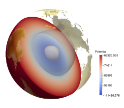
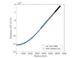
(a1)	(a2)
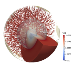
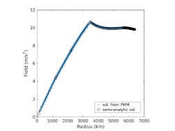
(b1)	(b2)

Figure 7: Comparison between the semi-analytical and FMM solutions: (a1) FMM gravitational potential; (a2) comparison in the radial direction; (b1) FMM gravitational field; (b2) comparison in the radial direction.

In Table 7, we show the approximation errors of different seven-layer models which contain six major discontinuities (Moho, top of Low Velocity Zone (LVZ), bottom of LVZ, 660, CMB and ICB) with the semi-analytical solution.

# of elements	2,031,729	5,018,249	8,043,617	12,479,828	16,560,615
MSE of $\Phi^{0}$	2.333e-7	4.485e-8	1.286e-8	9.785e-9	5.548e-9
MSE of $g$	1.926e-4	8.606e-5	5.186e-5	4.036e-6	3.394e-5

Table 7: Errors of seven-layer approximations in the gravitational calculation.

6.2 Computational accuracy for non-rotating planets

In this subsection, we do not consider rotation and study the computational accuracy with existing algorithms for spherically-symmetric planets. Let the angular velocity of rotation $\Omega=0$, without loss of generality, we write (54) and its pure solid planet version (50) in the form of generalized eigenvalue problems:

$$A\tilde{u}=\omega_{N}^{2}M\tilde{u},$$ (55)

where $A$ represents $A_{sg}-C_{s}^{\mathsf{T}}S_{s}C_{s}$ in (50) or $A_{G}-E_{G}A_{p}^{-1}E_{G}^{\mathsf{T}}-C^{\mathsf{T}}SC$ in (54) and $\omega_{N}$ denotes the frequency for the non-rotation planets. Since the explicit formation of $A$ with self-gravitation requires excessive storage, it is necessary to solve (55) via a matrix-free scheme, where $A$, $M$ and $M^{-1}$ are only accessed through matrix-vector multiplications. We combine several efficient parallel approaches to solve (55) with a matrix-free scheme.

In this work, we utilize polynomial filtering techniques saad:filtered-cr06 ; Filtlan-paper ; spectrumslicing as these do not involve solving linear systems with the indefinite matrices. Here, the bulk of computations are carried out in the form of matrix-vector products. The polynomial filtering technique is ideally suited for solving large-scale three-dimentional interior eigenvalue problems because it significantly enhances the memory and computational efficiency without any loss of accuracy DBLP:conf/sc/ShiLXSH18 . In this paper, we adopt the polynomial filtering algorithms recently developed in spectrumslicing ; DBLP:conf/sc/ShiLXSH18 ; li2019evsl due to their simplicity and robustness on a prescribed interval $[f_{1},f_{2}]$ mHz. The details about our parallel algorithms and their performance can be found in DBLP:conf/sc/ShiLXSH18 .

We show the convergence of our numerical formulation and approach for constant elastic balls and PREM. The constant balls have a radius of 6,371 km, density $\rho^{0}=5.51\times 10^{3}$ kg/$m^{3}$, P-wave speed $V_{P}$ = 10.0 km/s and S-wave speed $V_{S}$ = 5.7735 km/s. The PREM used in our tests is modified in an isotropic model without attenuation, with $V_{P}=(V_{PV}+V_{PH})/2$ and $V_{S}=(V_{SV}+V_{SH})/2$. The ocean layer in PREM is replaced by crust. In the work of Matchette-Downes2021 , a good agreement of the one-dimensional solution based on the classical approach MINEOS masters2011mineos and a radial FEM jingchen2018revisiting is demonstrated. The discretization of the radial FEM code is described in Appendix B, In this work, we show our three-dimensional results are in a good agreement with the one-dimensional solutions.

6.2.1 Solid models with self-gravitation

We present our results for purely solid models with self-gravitation. In Tables 8 and 10, we list the number of elements ‘#elm.’ as well as the problem sizes (labeled as ‘size of $A$’ for the solid cases and ‘size of $A_{G}$’ and ‘size of $A_{p}$’ for the Earth examples), the number of surfaces ‘#surf.’, the size of $S_{s}$ or $S$, and the target frequency interval in milliHertz (labeled as $[f_{1},f_{2}]$ (mHz)), the degree of the polynomial filter ‘deg’, the number of the Lanczos iterations required ‘#it’, and the number of the normal modes computed ‘#eigs’.

Exp.	#elm.	size of $A$	#surf.	size of $S_{s}$	$[f_{1},f_{2}]$ (mHz)	(deg,#it)	#eigs
C1p1	5,123	2,727	392	5,515	[0.1,1.0]	(14,192)	70
C2p1	21,093	10,644	956	22,049	[0.1,1.0]	(25,232)	92
C3p1	39,273	19,131	956	40,229	[0.1,1.0]	(34,252)	92
C4p1	105,115	51,933	3,608	108,723	[0.1,1.0]	(50,252)	92
C5p1	495,099	242,721	14,888	509,987	[0.1,1.0]	(108,272)	92

Table 8: Test cases with self-gravitation for different solid models using P1 elements for the frequency range $[0.1,1.0]$ mHz.

Since the pure solid models do not generate any essential spectra, we can directly compute the lowest-frequency normal modes. We note that the length ($\lambda_{\max}-\lambda_{\min}$) of the spectrum grows with the size of the problem determined by the discretization.

Exp.	${}_{0}T_{2}$	${}_{0}S_{2}$	${}_{1}S_{1}$	${}_{0}S_{0}$	${}_{0}T_{3}$	${}_{0}S_{3}$	${}_{1}S_{2}$	${}_{0}T_{4}$	${}_{0}S_{4}$
C1p1	0.3724	0.4178	0.4600	0.5105	0.5881	0.6322	0.6900	0.7973	0.8359
C2p1	0.3653	0.4112	0.4511	0.5053	0.5692	0.6052	0.6708	0.7587	0.7791
C3p1	0.3643	0.4103	0.4502	0.5053	0.5665	0.6017	0.6680	0.7527	0.7721
C4p1	0.3622	0.4089	0.4472	0.5035	0.5612	0.5932	0.6622	0.7424	0.7526
C5p1	0.3612	0.4086	0.4460	0.5035	0.5587	0.5899	0.6596	0.7374	0.7445
1D	0.3607	0.4087	0.4456	0.5040	0.5574	0.5885	0.6582	0.7348	0.7406

Table 9: Convergence tests with self-gravitation for different solid models in Table 8 with self-gravitation for P1 elements.

In Table 9, we show the convergence results for different solid models using P1 elements, that is, the finite-element polynomial orders $p^{s}=p^{f}=p^{p}=1$ are used throughout this work. Through comparison with 1D results, we observe that our computational results do converge. We accept relative differences of about 0.1%.

Exp.	# of elm.	size of $A$	#surf.	size of $S_{s}$	$[f_{1},f_{2}]$ (mHz)	(deg,#it)	#eigs
C1p2	19,073	75,888	956	20,029	[0.1,1.0]	(44,512)	92
C2p2	40,378	170,025	3,608	43,986	[0.1,1.0]	(58,492)	92
C3p2	80,554	335,103	5,924	86,478	[0.1,1.0]	(81,492)	92
C4p2	152,426	645,687	14,888	167,314	[0.1,1.0]	(129,492)	92
C5p2	334,193	1,360,140	14,888	349,081	[0.1,1.0]	(200,492)	92

Table 10: Test cases with self-gravitation for different solid models using P2 elements for the frequency range $[0.1,1.0]$ mHz.

Exp.	${}_{0}T_{2}$	${}_{0}S_{2}$	${}_{1}S_{1}$	${}_{0}S_{0}$	${}_{0}T_{3}$	${}_{0}S_{3}$	${}_{1}S_{2}$	${}_{0}T_{4}$	${}_{0}S_{4}$
C1p2	0.3619	0.4100	0.4473	0.5094	0.5594	0.5908	0.6605	0.7376	0.7439
C2p2	0.3610	0.4090	0.4459	0.5042	0.5579	0.5889	0.6587	0.7355	0.7413
C3p2	0.3609	0.4089	0.4463	0.5042	0.5577	0.5888	0.6585	0.7352	0.7410
C4p2	0.3608	0.4088	0.4456	0.5041	0.5575	0.5886	0.6583	0.7349	0.7408
C5p2	0.3608	0.4087	0.4456	0.5041	0.5575	0.5885	0.6583	0.7349	0.7407
1D	0.3607	0.4087	0.4456	0.5040	0.5574	0.5885	0.6582	0.7348	0.7406

Table 11: Convergence tests with self-gravitation for the solid models in Table 10 using P2 elements.

In Table 10, we list test cases for different solid models using P2 elements, that is, the finite-element polynomial orders $p^{s}=p^{f}=p^{p}=2$ are used throughout this work. From experiments C1p2 to C5p2, we double the number of elements and obtain proper convergence results in Table 11. We show that even with about 330,000 elements, we are able to achieve four-digit agreement.

6.2.2 PREM with self-gravitation

Here, we include a liquid outer core using PREM and the presence of the essential spectrum. In Table 12, we show test cases for PREM. We roughly double the number of elements from E1p1 to E7p1. In Table 13, we argue convergence by comparing with 1D results. For PREM with self-gravitation, we accept relative differences that are less than 0.1%.

Exp.	# of elm.	size of $A_{G}$	size of $A_{p}$	#surf.	size of $S$	$[f_{1},f_{2}]$ (mHz)	(deg,#it)	#eigs
E1p1	9,721	7,590	887	2,304	12,025	[0.1,1.0]	(187,392)	64
E2p1	20,466	14,736	974	4,956	25,422	[0.1,1.0]	(182,372)	72
E3p1	42,828	30,384	3,171	8,172	51,000	[0.1,1.0]	(342,452)	83
E4p1	83,354	63,225	5,298	22,104	105,458	[0.1,1.0]	(745,452)	88
E5p1	157,057	96,852	6,771	22,104	179,161	[0.1,1.0]	(747,492)	88
E6p1	303,218	164,673	10,077	22,104	325,322	[0.1,1.0]	(685,492)	88
E7p1	639,791	361,587	21,824	60,288	700,079	[0.1,1.0]	(685,492)	88
E8p1	1,972,263	1,086,702	70,429	150,288	2,122,551	[0.1,1.0]	(1565,492)	88
E8p2	1,972,263	8,400,630	522,705	150,288	2,122,551	[0.3,1.5]	(1185,1051)	268

Table 12: Test cases with self-gravitation for different Earth models E1p1 - E8p1 using P1 elements for the frequency range $[0.1,1.0]$ mHz and Earth model E8p2 using P2 elements for the frequency range $[0.3,1.5]$ mHz.

Exp.	${}_{0}S_{2}$	${}_{0}T_{2}$	${}_{2}S_{1}$	${}_{0}S_{3}$	${}_{0}T_{3}$
E1p1	0.3284	0.3953	0.4179	0.5242	0.6241
E2p1	0.3229	0.3921	0.4149	0.5077	0.6146
E3p1	0.3177	0.3884	0.4113	0.4932	0.6062
E4p1	0.3166	0.3842	0.4090	0.4903	0.5980
E5p1	0.3137	0.3845	0.4085	0.4863	0.5962
E6p1	0.3126	0.3840	0.4080	0.4768	0.5945
E7p1	0.3116	0.3834	0.4073	0.4742	0.5933
E8p1	0.3112	0.3829	0.4067	0.4721	0.5920
E8p2	0.3106	0.3826	0.4063	0.4708	0.5912
1D	0.3110	0.3826	0.4063	0.4713	0.5912

Table 13: Convergence tests with self-gravitation for different Earth models in Table 12.

6.3 Fully heterogeneous models

Here, we study the effects of heterogeneity on the normal modes. In Subsection 6.3.2 and Subsection 6.3.1, we study the effects of the crust and upper mantle, and shape of the CMB, respectively.

6.3.1 Shape of the CMB

Exp.	# of elm.	size of $A_{G}$	size of $A_{p}$	#surf.	size of $S$	$[f_{1},f_{2}]$ (mHz)	(deg,#it)	#eigs
CMB8	2,007,479	8,711,940	633,358	177,352	2,184,831	[1.5,2.0]	(3591,1251)	350

Table 14: Test case with self-gravitation for an Earth model with a non-spherically symmetric CMB using P2 elements.

Here, we study the effects of the CMB. Long-wavelength topography of the CMB was proposed by creager1986aspherical ; morelli1987topography . Many studies bataille1988inhomogeneities ; doornbos1989models ; pulliam1993bumps ; rodgers1993inference ; obayashi1997p ; earle1997observations ; earle1998observations ; garcia2000amplitude ; sze2003core ; lassak2010core ; tanaka2010constraints ; colombi2014seismic ; schlaphorst2015investigation were later performed to model the topography of the CMB.

In Fig. 8, we show the topography of the CMB from the result by tanaka2010constraints . We use a triangular mesh to model the shape with ellipticity combined. In Table 14, we show the information of the experiment CMB8, which indicates a PREM-like model with the mentioned CMB embedded. In Fig. 9, we illustrate the splittings of modes ${}_{1}S_{7}$ and ${}_{1}S_{8}$ due to the non-spherically symmetric CMB. Since the modes ${}_{1}S_{7}$ and ${}_{1}S_{8}$ are sensitive to the change of the CMB, the splittings of these modes are quite clear.

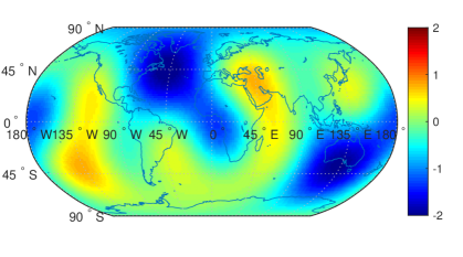
Figure 8: Shape of the CMB using the result of tanaka2010constraints . The values in the color bar indicate the variations in kilometers.

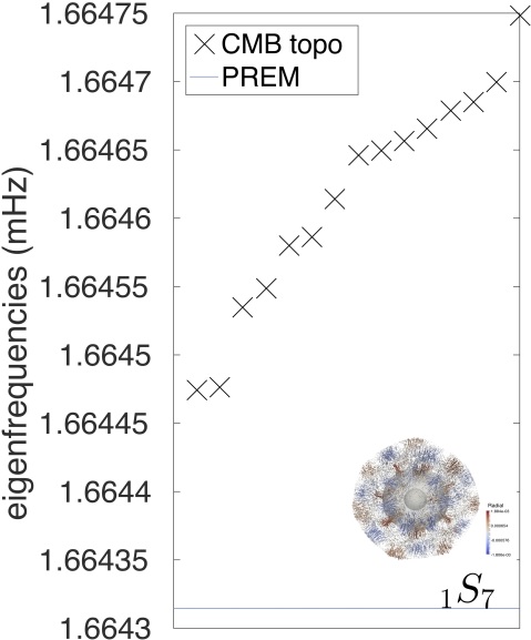
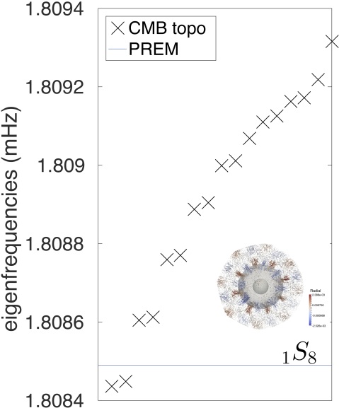
Figure 9: Splittings of the modes ${}_{1}S_{7}$ and ${}_{1}S_{8}$ due to the non-spherically symmetric CMB, which is shown in Figs. 8.

6.3.2 Heterogeneity of the crust and upper mantle

Self-gravitation is important for the normal modes with frequencies lower than 5.0 mHz or so kennett1998density . However, in this subsection, we restrict ourselves to models without perturbation of the gravitational potential for computational efficiency. We reduce the full generalized eigenvalue problem (55) into Cowling approximation

$$(A_{G}-E_{G}A_{p}^{-1}E_{G}^{\mathsf{T}})\tilde{u}=\omega_{C}^{2}M\tilde{u},$$ (56)

where $\omega_{C}$ is the frequency for Cowling approximation.

Exp.	# of elm.	size of $A_{G}$	size of $A_{p}$	$[f_{1},f_{2}]$ (mHz)	(deg,#it)	#eigs
E9p2	4,094,031	17,469,666	1,181,103	$[2.0,2.5]$	(4054,1892)	528
MIT_2016May	4,048,932	16,578,945	879,067	$[2.0,2.5]$	(2674,1912)	520
MIT+crust 1.0	4,044,225	16,550,922	878,808	$[2.0,2.5]$	(6984,1912)	550

Table 15: Test cases for four different Earth models using the Cowling approximation.

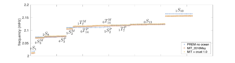
(a)

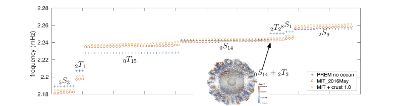
(b)

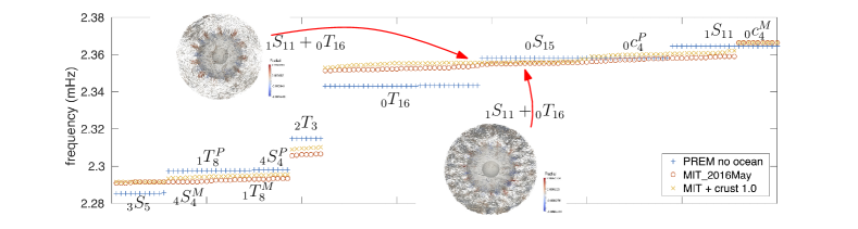
(c)

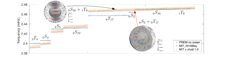
(d)

Figure 10: Comparisons between different Earth models in the Cowling approximation. The results from PREM without ocean, the MIT model, and the MIT model with the three-dimensional crust are shown using blue $+$, red $\circ$ and yellow $\times$, respectively. The superscripts $P$, $M$ on the mode symbols denote PREM and MIT models, respectively. (a-d) Comparison for different modes in $[2.0,2.18]$, $[2.18,2.28]$, $[2.28,2.38]$ and $[2.38,2.48]$ mHz, respectively. The mode in (b) couples ${}_{0}S_{14}$ with ${}_{2}T_{2}$. The two modes in (c) couple ${}_{1}S_{11}$ with ${}_{0}T_{16}$. The left mode in (d) couples ${}_{0}S_{16}$ with ${}_{1}T_{9}$. The right mode in (d) couples ${}_{6}S_{2}$ with ${}_{0}T_{17}$.

In Table 15, we show three different Earth models using the Cowling approximation. We construct two three-dimensional Earth models using MIT’s mantle tomographic results burdick2017model and crust 1.0 laske2013update . The core model is based on PREM. The mantle seismic reference wave speeds are based on AK135 kennett1995constraints . One model is obtained by combining MIT’s mantle tomographic model and PREM for the core and density. The other one replaces PREM’s crust by crust 1.0, which is shown in Fig. 3. In the first three rows of Table 15, we show the information of three different tests for these three different Earth models. Since with similar degrees of freedom, the largest eigenvalue of the MIT model with the three-dimensional crust is much larger than these of the other two models, we expect that significant mode coupling and splitting occur deuss2001theoretical ; romanowicz2008computation ; beghein2008signal ; irving2009normal ; koelemeijer2012normal ; nader2015normal ; yang2015synthetic ; akbarashrafi2017exact ; al2018hamilton .

We visualize different modes. The normal modes computed in the two MIT models are non-degenerate. In Fig. 10, we compare different modes computed in the three models in the frequency range $[2.0,2.5]$ mHz. Since the background models have only slight differences, some of the eigenfrequencies are similar amongst PREM and the MIT models. We illustrate most of the modes computed in PREM. In Fig. 10 (a), we observe that, even at low frequencies, weak mode splitting occurs for surface wave modes, including ${}_{2}S_{8}$, ${}_{0}S_{13}$, ${}_{0}T_{14}$ and ${}_{1}T_{7}$. We also report that no coupled modes are observed in $[2.0,2.18]$ mHz. In Figs. 10 (b-d), we show the different modes in $[2.18,2.28]$, $[2.28,2.38]$ and $[2.38,2.48]$ mHz, respectively. The splitting of most surface wave modes becomes larger with increasing frequency. However, since modes like ${}_{1}S_{10}$ (strong at the core-mantle boundary) in Fig. 10 (a), ${}_{0}c_{4}$ (an inner core toroidal mode) and ${}_{3}S_{5}$ (an ICB Stoneley mode) in Fig. 10 (c), are not sensitive to the crust and upper mantle structure, no clear splitting is observed. We observe coupled modes in Figs. 10 (b-d) computed in the MIT model with the three-dimensional crust. The eigenfunction of one mode in Fig. 10 (b) shows that ${}_{0}S_{14}$ and ${}_{2}T_{2}$ are coupled. The ${}_{0}T_{15}$ and ${}_{8}S_{1}$ near ${}_{0}S_{14}$ and ${}_{2}T_{2}$ are isolated multiplets. The eigenfunctions of the two modes in Fig. 10 (c) show that ${}_{1}S_{11}$ and ${}_{0}T_{16}$ are coupled. The ${}_{0}S_{15}$ near ${}_{1}S_{11}$ and ${}_{0}T_{16}$ is an isolated multiplet. These coupled modes are interesting because ${}_{1}S_{11}$ is clearly sensitive to the core-mantle boundary and the fundamental Love mode ${}_{0}T_{16}$ illustrated can be measured at the surface. The left mode in Fig. 10 (d) is a ${}_{0}S_{16}$ and ${}_{1}T_{9}$ coupled mode. The right mode in Fig. 10 (d) is a ${}_{6}S_{2}$ and ${}_{0}T_{17}$ coupled mode. This mode is also very interesting because ${}_{6}S_{2}$ illustrated is an inner core mode and the fundamental Love mode ${}_{0}T_{17}$ illustrated can be detected at the surface. Since the relative wave speed variations of the MIT tomographic model vary roughly from -1.4% to 1.4% in the upper mantle and the crust’s thickness is small, strong mode coupling occurs only to two modes. In this frequency range $[2.0,2.5]$ mHz, the width of each multiplet is small and no significant coupling between three or more modes is observed.

7 Computational experiments for rotating planets

In this section, we include the rotation and study its effects on normal modes. To simplify (54) and (50) without any loss of the generality, we extend (55) and derive a standard form for the QEP,

$$\omega^{2}M\tilde{u}-2\operatorname{i}\omega\tilde{R}_{\Omega}\tilde{u}-A\tilde{u}=0.$$ (57)

We note that $\tilde{R}_{\Omega}=-\tilde{R}^{\mathsf{T}}_{\Omega}$, that is, $2\operatorname{i}\tilde{R}_{\Omega}$ is Hermitian. The eigenfrequencies are real and come in pairs $(\omega,-\omega)$.

To solve the QEP of the original form, the QEP is often projected onto a properly chosen low-dimensional subspace to facilitate the reduction to a QEP directly of lower dimension, such as in the Jacobi–Davidson method sleijpen1996jacobi ; sleijpen1996quadratic . The reduced QEP can then be solved by a standard dense matrix technique. Both Arnoldi- and Lanczos-type processes hoffnung2006krylov have been developed to build such projections of the QEP. A subspace approximation method holz2004subspace was presented via applying perturbation theory to the QEP. A second-order Arnoldi procedure bai2005soar was developed to generate an orthonormal basis for solving a large-scale QEP directly. We note that the above mentioned methods typically utilize a shift-and-invert scheme for solving the interior eigenpairs. These techniques become impractical for eigenvalue problems of the size of ours due to the high memory costs.

Instead, we can utilize extended Lanczos vectors from solving the generalized eigenvalue problem (55) through the polynomial filtering method. We then approximate the solution $\tilde{u}$ using the basis computed from

$$AX_{e}=MX_{e}\Lambda_{e},$$ (58)

where $X_{e}$ stands for the Ritz vectors of the linear system and $\Lambda_{e}$ denotes a diagonal matrix whose diagonal is a collection of $\omega_{N}^{2}$ in (55). We take $m_{e}$ eigenvectors spanning a subspace and let $\tilde{u}_{e}=X_{e}y_{e}$ approximate $\tilde{u}$ in (57), where $y_{e}$ is complex. We apply

$$\left(\begin{array}[]{cc}X_{e}^{\mathsf{T}}&0\\ 0&X_{e}^{\mathsf{T}}\end{array}\right)$$

to an equivalent form of (57),

$$\left(\begin{array}[]{cc}0&A\\ A&2\operatorname{i}\tilde{R}_{\Omega}\end{array}\right)\left(\begin{array}[]{c}\tilde{u}\\ \omega\tilde{u}\end{array}\right)=\omega\left(\begin{array}[]{cc}A&0\\ 0&M\end{array}\right)\left(\begin{array}[]{c}\tilde{u}\\ \omega\tilde{u}\end{array}\right).$$

Making use of $X_{e}^{\mathsf{T}}AX_{e}=\Lambda_{e}$, we obtain

$$\left(\begin{array}[]{cc}0&\Lambda_{e}\\ \Lambda_{e}&2\operatorname{i}X_{e}^{\mathsf{T}}\tilde{R}_{\Omega}X_{e}\end{array}\right)\left(\begin{array}[]{c}y_{e}\\ \omega_{e}y_{e}\end{array}\right)=\omega_{e}\left(\begin{array}[]{cc}\Lambda_{e}&0\\ 0&I\end{array}\right)\left(\begin{array}[]{c}y_{e}\\ \omega_{e}y_{e}\end{array}\right).$$ (59)

It is apparent that if $\tilde{R}_{\Omega}=0$, we have $\omega_{e}=\omega_{N}=\Lambda_{e}^{1/2}$. The system (59) can be solved with a standard eigensolver such as the one implemented in LAPACK anderson1999lapack . Here, we study the spectra of two models: Earth 1066A gilbert1975application and a Mars model khan2016single . We use 23.9345 hours allen1973astrophysical and 24.6229 hours lodders1998planetary as Earth’s and Mars’ rotation periods, respectively. With a large $m_{e}$ and a relatively small $\Omega$, the numerical solution $\omega_{e}$ is close to $\omega$ in (57). The numerical accuracy can further be improved via solving (57) exactly.

7.1 Computational accuracy

Exp.	# of elm.	size of $A$	size of $A_{p}$	size of $S$	$[f_{1},f_{2}]$ (mHz)
Constant (C3kp1)	3,129	1,821	0	3,521	[0.35,0.85]
Earth (E3kp1)	3,330	2,760	392	4,242	[0.3,0.86]
Mars (M2kp1)	1,887	1,677	145	2,539	[0.4,1.14]
Mars (M8kp1)	8,020	7,557	152	12,436	[0.4, 1.14]
Earth (E40kp1)	42,828	30,384	3,171	51,000	[0.1,1.5]

Table 16: Numerical parameter values pertaining to the testing of computational accuracy and estimating the cost in different models.

For small models, we are able to compute the full mode expansion associated with the point spectrum using (59). In Table 16, we list the numerical parameter values pertaining to the testing of computational accuracy and estimating the cost in different models: The number of elements (labeled as # of elm.), size of $A_{p}$, size of $A$, size of $S$ and the target frequency interval in milliHertz (labeled as $[f_{1},f_{2}]$ (mHz)).

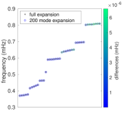
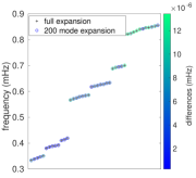
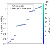
(a) Constant (C3kp1)	(b) Earth (E3kp1)	(c) Mars (M2kp1)

Figure 11: Tests with three different small models for the low-frequency seismic eigenfrequencies. The numerical parameters of the tests are given in Table 16.

In Figs. 11 (a)–(c), we illustrate the computational accuracy of tests in three different models, C3kp1, E3kp1 and M2kp1, respectively, on the lowest seismic eigenfrequencies using P1 elements. We compare the differences in the eigenfrequencies between the full mode expansion and a 200 mode expansion. The differences are about $5\times 10^{-6}$ mHz, which is two digits below the accuracy of common normal mode measurements.

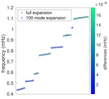
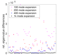
(a) M8kp1 on [0.4, 1.14] mHz	(b) Errors of (a)

Figure 12: Tests for computational accuracy of a Mars model using different numbers of mode expansion.

In Figs. 12 (a) and (b), we show the computational accuracy of M8kp1 on [0.4, 1.14] mHz as well as the error distribution. In Fig. 12 (a), we show that even with a 100 mode expansion, the differences are as low as $1\times 10^{-5}$ mHz. In Fig. 12 (b), we show that with a 1000 mode expansion, the differences are further reduced to about $1\times 10^{-6}$ mHz.

7.2 Benchmark experiments for Earth models with rotation

Over the past two decades, a significant number of observational studies have been carried out to the rotation effects on the Earth’s normal modes zurn2000observation ; millot2003normal ; park2005earth ; roult2010observation ; nader2015normal ; schimmel2018low . Our computational approach can aid and complement such studies through accurate and consistent simulations generating even relatively high eigenfrequencies. Here, we perform a benchmark experiment of Earth model 1066A gilbert1975application against a perturbation calculation dahlen1979rotational . In the perturbation calculation, the eigenfrequency perturbations $\delta\omega_{m}$ have the following form

$$\delta\omega_{m}=\omega_{0}(a+bm+cm^{2}),\quad-l\leq m\leq l,$$ (60)

where $\omega_{0}$ denotes the eigenfrequency of the unperturbed spherically symmetric model, $l$ denotes the angular order in the spherical harmonic expansion, and $a$, $b$ and $c$ are the relevant coefficients. The values of $a$, $b$ and $c$ for different radial modes can be found in (dahlen1998theoretical, , Table 14.1). In Table 17, we list the numerical parameters of the Earth models in the benchmark test. The models E1Mp1 and E2Mp2 used to compute $\omega_{0}$ represent spherically symmetric ones without rotation. Experiments EE1Mp1 and EE2Mp2 represent elliptic Earth models and are used to compute eigenfrequencies with our proposed method. The ellipticities of the Earth models are computed by solving Clairaut’s equation (cf. Section 3). Since the eigenfrequencies of the Slichter modes slichter1961fundamental are close to the upper bound of the essential spectrum and the convergence of the proposed algorithm is relatively slow, we set $f_{1}=$ 0.04 mHz and use experiments E1Mp1 and EE1Mp1 to compute the Slichter modes using P1 elements. Experiments E2Mp2 and EE2Mp2 are used to compute other modes using P2 elements. In Fig. 13, we show the comparison between the perturbation and our methods. The values of the computed eigenfrequenies of our method agree with the perturbation results in as much as that the relative differences are commonly less than 0.3 $\mu$Hz. The degree of agreement is, of course, model dependent. The eccentricity in the Earth model is so small that the second-order perturbation is accurate within the typical error of our numerical computations. Higher rotation rates would increase the eccentricity and let the second-order perturbation loose accuracy.

Exp.	# of elm.	size of $A$	size of $A_{p}$	size of $S$	$[f_{1},f_{2}]$ (mHz)
Earth (E1Mp1)	1,011,973	537,198	31,849	1,074,577	[0.04,1.5]
Earth (E2Mp2)	2,015,072	8,569,197	530,721	2,165,360	[0.2,1.5]
Earth (EE1Mp1)	1,003,065	533,064	31,688	1,065,629	[0.04,1.5]
Earth (EE2Mp2)	2,002,581	8,520,432	528,124	2,153,109	[0.2,1.5]

Table 17: Numerical parameters of the Earth models used in the benchmark experiments.

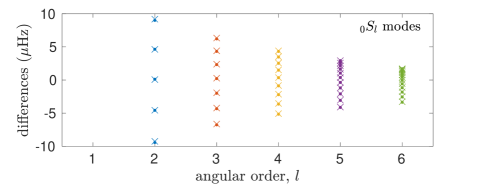
(a) Comparison of ${}_{0}S_{l}$ modes

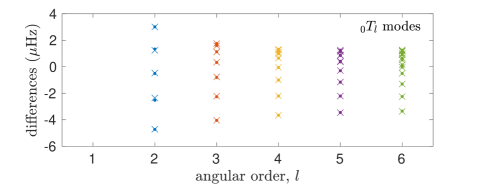
(b) Comparison of ${}_{0}T_{l}$ modes

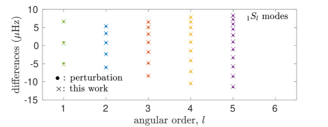
(c) Comparison of ${}_{1}S_{l}$ modes

Figure 13: Comparison of the results from a perturbation calculation and our proposed method, which are shown using symbols $\bullet$ and $\times$, respectively. (a), (b) and (c) illustrate comparisons of ${}_{0}S_{l}$, ${}_{0}T_{l}$ and ${}_{1}S_{l}$ modes, respectively.

7.3 Mars models

Here, we present our computational results for Mars models. The interiors of the Mars models are based on mineral physics calculations khan2016single . In Table 18, we list three Mars models labeled as M2Mp2, EM2Mp2 and TM2Mp2 which represent a spherically symmetric Mars model without rotation, a spheroidal Mars model with rotation, and a spheroidal Mars model with a three-dimensional crust and rotation using P2 elements. The shape of the spheroidal Mars model’s core-mantle boundary is computed by solving Clairaut’s equation. Since Mars presumably is not hydrostatic as discussed in Section 3, its solid region is estimated via a linear interpolation using the ellipticities of the core-mantle boundary ($\varepsilon=4.19\times 10^{-3}$) and the surface ($\varepsilon=5.89\times 10^{-3}$). Model TM2Mp2 is illustrated in Fig. 5.

Exp.	# of elm.	size of $A$	size of $A_{p}$	size of $S$	$[f_{1},f_{2}]$ (mHz)
Mars (M2Mp2)	1,996,773	8,967,684	579,338	2,257,801	[0.2,2.0]
Mars (EM2Mp2)	2,001,619	8,984,532	579,667	2,262,143	[0.2,2.0]
Mars (TM2Mp2)	2,008,654	8,289,927	323,810	2,158,366	[0.2,2.0]

Table 18: Numerical parameters for the Mars models.

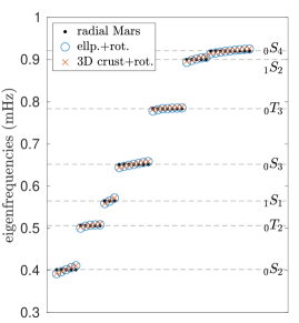
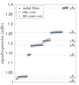
(a) modes in [0.3, 1.0]mHz	(b) modes in [1.0, 1.4]mHz
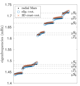
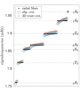
(c) modes in [1.4, 1.75]mHz	(d) modes in [1.75, 1.95]mHz

Figure 14: Eigenfrequencies of different Mars models. (a), (b), (c) and (d) illustrate eigenfrequencies in different frequency windows. Symbols $\bullet$, $\circ$ and $\times$ represent the eigenfrequencies computed from Mars models M2Mp2, EM2Mp2 and TM2Mp2 in Table 18, respectively. The x-axis indicates the indexes of eigenfrequencies with ascending order. The horizontal dashed lines represent the eigenfrequencies of a spherically symmetric Mars model computed with a one-dimensional solver.

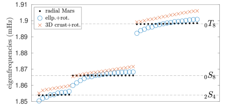
Figure 15: Illustration of a subinterval in Fig. 14 (d). The x-axis indicates the indexes of eigenfrequencies with ascending order. Splitting of modes ${}_{2}S_{4}$, ${}_{0}S_{8}$, and ${}_{0}T_{8}$ due to the three-dimensional crust. The maximum difference between the eigenfrequencies is 5.2 $\mu$Hz.

In Fig. 14, we show eigenfrequencies computed in different Mars models listed in Table 18. Symbols $\bullet$, $\circ$ and $\times$ represent the eigenfrequencies computed in Mars models M2Mp2, EM2Mp2 and TM2Mp2 (cf. Table 18). The horizontal dashed lines represent the eigenfrequencies of a spherically symmetric Mars model computed with a one-dimensional solver masters2011mineos ; jingchen2018revisiting . Mode splitting is apparent due to ellipticity, rotation and heterogeneity in three dimensions. The three-dimensional crust does not have a clear influence on the lowest eigenfrequencies associated with ${}_{0}S_{2}$, ${}_{0}T_{2}$, ${}_{1}S_{1}$, ${}_{0}S_{3}$, ${}_{0}T_{3}$, ${}_{1}S_{2}$ and ${}_{0}S_{4}$ in Fig. 14 (a). The three-dimensional crust has a noticeable effect on the surface wave modes, such as ${}_{0}T_{6}$, ${}_{0}T_{7}$, ${}_{0}T_{8}$, ${}_{0}S_{6}$, ${}_{0}S_{7}$ and ${}_{0}S_{8}$, as expected. In Fig. 15, we show the eigenfrequencies in a subinterval of the interval used in Fig. 14 (d). Here, we note the splitting of modes ${}_{2}S_{4}$, ${}_{0}S_{8}$ and ${}_{0}T_{8}$ and highlight the effects of the three-dimensional crust. The maximum difference between the eigenfrequencies in Fig. 15 is 5.2 $\mu$Hz, which, in principle, can be detected. There is no mode-coupling observed in these experiments.

In Fig. 16, we plot the branch ${}_{1}S_{l}$ as well as the corresponding incremental gravitational fields $\nabla S(u)$. The superconducting gravimeters are expected to contribute to normal mode seismology crossley1999network ; van1999measuring ; widmer2003can ; rosat2003search ; hafner2012signature . We anticipate that both the seismic and gravity measurements of these modes could help to estimate the size of the Martian core.

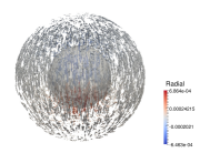
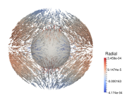
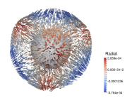
(a1) ${}_{1}S_{1}$	(a2) ${}_{1}S_{2}$	(a3) ${}_{1}S_{3}$
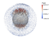
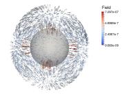
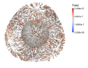
(b1) $\nabla S(u)$ of ${}_{1}S_{1}$	(b2) $\nabla S(u)$ of ${}_{1}S_{2}$	(b3) $\nabla S(u)$ of ${}_{1}S_{3}$
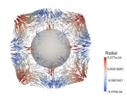
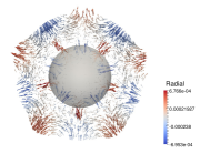
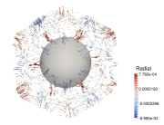
(a4) ${}_{1}S_{4}$	(a5) ${}_{1}S_{5}$	(a6) ${}_{1}S_{6}$
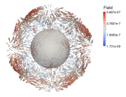
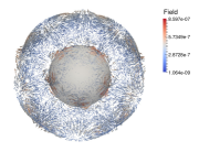
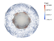
(b4) $\nabla S(u)$ of ${}_{1}S_{4}$	(b5) $\nabla S(u)$ of ${}_{1}S_{5}$	(b6) $\nabla S(u)$ of ${}_{1}S_{6}$

Figure 16: Visualization of ${}_{1}S_{l}$ branch of a Mars model with a three-dimensional crust and rotation from TM2Mp2 experiment. The light ball indicates the position of the core-mantle boundary. (a1)–(a6) illustrate the modes ${}_{1}S_{1}$ to ${}_{1}S_{6}$, respectively. The unit in the color of (a1) - (a6) is meter. (b1)–(b6) illustrate the perturbed gravitational field $\nabla S(u)$ of the modes ${}_{1}S_{1}$ to ${}_{1}S_{6}$, respectively. The unit in the colorbar of (b1)–(b6) is millimeter.

8 Conclusion

In this work, we propose a method to compute the normal modes of a fully heterogeneous rotating planet. We apply the mixed finite-element method to the elastic-gravitational system of a rotating planet and utilize the FMM to calculate the self-gravitation. We successfully separate out the essential spectrum by using a polynomial filtering eigensolver and thus, are able to compute the normal modes associated with seismic point spectrum. To solve the relevant QEP, we utilize extended Lanczos vectors computed in a non-rotating planet – with the shape of boundaries of a rotating planet and accounting for the centrifugal potential – spanning a subspace to reduce the dimension of an equivalent linear form of the QEP. The reduced system can be solved with a standard eigensolver. We demonstrate our ability to compute the seismic normal modes with and without rotation accurately. We then study the computational accuracy and use a standard Earth model to perform a benchmark test against a perturbation calculation. We carry out computational experiments on various Mars models and illustrate mode splitting due to rotation, ellipticity and heterogeneity of the crust. The use of modern supercomputers enables us to capture normal modes associated with the seismic point spectrum of a fully heterogeneous planet accurately. The computational efficiency can be further improved by using acceleration techniques. The extension to include viscoelastic relaxation (for a review, see romanowicz20071 ), in particular Maxwell and Burger models, leads to a nonlinear rational eigenvalue problem, which is tractable at current subject of research.

Appendix A Construction of orthonormal bases and submatrices

Here, we introduce three-dimensional polynomial bases $\{\psi_{n}^{s}\}_{n=1}^{N_{p^{s}}}$, $\{\psi_{n}^{f}\}_{n=1}^{N_{p^{f}}}$ and $\{\psi_{n}^{p}\}_{n=1}^{N_{p^{p}}}$ while addressing the fact that the Lagrange polynomials are not orthogonal to one another. We suppress superscripts $s$, $f$, $p$ in the notation in the remainder of this subsection. To simplify the computations, we introduce reference volume and boundary elements. That is, we introduce a mapping that connects any element $K$ to the reference tetrahedron defined by

$$\mathbf{I}=\{r=(r_{1},r_{2},r_{3})\ :\ r_{1}\geq-1,\ r_{2}\geq-1,\ r_{3}\geq-1,\ r_{1}+r_{2}+r_{3}\leq-1\}.$$

Likewise, we introduce a mapping that connects any boundary element $E$ to the reference triangle defined by

$$\mathbf{I}_{2D}=\{t=(t_{1},t_{2})\ :\ t_{1}\geq-1,\ t_{2}\geq-1,\ t_{1}+t_{2}\leq 0\}.$$

We note that any two tetrahedra are connected through an affine transformation, $x\to r$, with a constant Jacobian, $J$, which is the determinant of $(\partial_{r}x)$. For the local approximation on the reference element $\mathbf{I}$, we have

$$u_{j}(r)=\sum_{n=1}^{N_{p}}(\hat{u}_{j})_{n}\psi_{n}(r)=\sum_{i=1}^{N_{p}}u_{j}(r_{i})\ell_{i}(r).$$

The vector fields are treated component-wise in our discretization. This yields the expression $\mathcal{V}\hat{u}_{j}=u_{j}$, where the generalized Vandermonde matrix takes the form of $\mathcal{V}_{in}=\psi_{n}(r_{i})$ with $i,n$ as indices of nodal points. Here, $\{\psi_{n}\}$ is a polynomial basis that is orthonormal on $\mathbf{I}$. We later introduce submatrices of $\mathcal{V}$. We then evaluate derivatives and mass matrices according to

$$\partial_{x_{i}}=(\partial_{x_{i}}r_{j})\mathcal{D}_{j},\quad\mathcal{D}_{j}=(\partial_{r_{j}}\mathcal{V})\mathcal{V}^{-1},\quad\mathcal{M}=\mathcal{V}^{-T}\mathcal{V}^{-1},$$

where $\mathcal{D}_{j}$ and $\mathcal{M}$ are the derivative matrix and the mass matrix on the reference tetrahedron. More details of the constructions of $J$, $\mathcal{V}$, $\mathcal{D}_{j}$ and $\mathcal{M}$ can be found in (hesthaven2007nodal, , Chapter 10.1). Thus, we introduce

$$\mathcal{V}_{s},\ \mathcal{V}_{f},\ \mathcal{V}_{p},\quad\mathcal{M}_{s},\ \mathcal{M}_{f},\ \mathcal{M}_{p}\quad\text{and}\quad\mathcal{D}_{j}^{s},\ \mathcal{D}_{j}^{f},\ \mathcal{D}_{j}^{p}.$$

We employ the notation

$$\mathsf{D}^{s}_{i}=(\partial_{x_{i}}r_{j})\mathcal{D}^{s}_{j},\quad\mathsf{D}^{f}_{i}=(\partial_{x_{i}}r_{j})\mathcal{D}^{f}_{j},\quad\mathsf{D}^{p}_{i}=(\partial_{x_{i}}r_{j})\mathcal{D}^{p}_{j},$$

reflecting the mapping of the derivatives from the reference tetrahedron to the target element. We follow a similar approach for boundary elements and introduce

$$\mathcal{M}_{s}^{2D},\ \mathcal{M}_{f}^{2D}\quad\text{and}\quad J^{2D},$$

where $\mathcal{M}_{s}^{2D}$ and $\mathcal{M}_{f}^{2D}$ are the mass matrices for solid and fluid boundary elements, respectively; $J^{2D}$ denotes the Jacobian, which is the determinant of $(\partial_{t}x)$ on the boundary element. The construction of the mass matrices $\mathcal{M}^{2D}_{s}$ and $\mathcal{M}^{2D}_{f}$ on the reference triangle $\mathbf{I}_{2D}$ is similar to the construction of $\mathcal{M}$ (hesthaven2007nodal, , Chapter 6.1).

A.1 Submatrices: $A_{sg}$, $A_{f}$, $A_{p}$, $M_{s}$, $M_{f}$, $R_{s}$ and $R_{f}$

We extract $\tilde{u}^{s}|_{K_{k}}$, $\tilde{u}^{f}|_{K_{k}}$ and $\tilde{p}|_{K_{k}}$ from $\tilde{u}^{s}$, $\tilde{u}^{f}$ and $\tilde{p}$, respectively, by restricting the nodes to the ones of element $K_{k}$. In a similar fashion, we extract $\tilde{v}^{s}|_{K_{k}}$, $\tilde{v}^{f}|_{K_{k}}$ and $\tilde{v}^{p}|_{K_{k}}$ on any element $K_{k}$. For the evaluation of matrix $A_{sg}$ in Table 3 we need to evaluate the submatrices on element $K_{k}$ through

$$\int_{K_{k}^{\text{S}}}\partial_{x_{i}}(\overline{v}^{s}_{h})_{j}(c_{ijmn}\partial_{x_{m}}(u^{s}_{h})_{n})\,\mathrm{d}x =(\tilde{v}^{s}_{j}|_{K_{k}})^{\mathsf{H}}[J_{k}(\mathsf{D}_{i}^{s})^{\mathsf{T}}c^{k}_{ijmn}\mathcal{M}_{s}\mathsf{D}_{m}^{s}]\tilde{u}^{s}_{n}|_{K_{k}},$$ (61)

$$\int_{K_{k}^{\text{S}}}\partial_{x_{i}}(\overline{v}^{s}_{h})_{i}g^{\prime}_{j}(u^{s}_{h})_{j}\rho^{0}\,\mathrm{d}x =(\tilde{v}^{s}_{i}|_{K_{k}})^{\mathsf{H}}[J_{k}(\mathsf{D}_{i}^{s})^{\mathsf{T}}\rho^{0}_{k}\mathcal{M}_{s}D_{g^{\prime}_{j}}]\tilde{u}^{s}_{j}|_{K_{k}},$$ (62)

$$\int_{K_{k}^{\text{S}}}-(u^{s}_{h})_{i}\partial_{x_{i}}g^{\prime}_{j}(\overline{v}^{s}_{h})_{j}\rho^{0}\,\mathrm{d}x =(\tilde{v}^{s}_{i}|_{K_{k}})^{\mathsf{H}}[-J_{k}\rho^{0}_{k}D_{\partial_{x_{i}}g^{\prime}_{j}}\mathcal{M}_{s}]\tilde{u}^{s}_{j}|_{K_{k}},$$ (63)

$$\int_{K_{k}^{\text{S}}}-(u^{s}_{h})_{j}(\partial_{x_{j}}(\overline{v}^{s}_{h})_{i})g^{\prime}_{i}\rho^{0}\,\mathrm{d}x =(\tilde{v}^{s}_{i}|_{K_{k}})^{\mathsf{H}}[-J_{k}\mathsf{D}^{s}_{j}\mathcal{M}_{s}\rho^{0}_{k}D_{g^{\prime}_{i}}]\tilde{u}^{s}_{j}|_{K_{k}},$$ (64)

where $c^{k}_{ijmn}$, $\rho^{0}_{k}$ and $J_{k}$ denote the stiffness tensor, density and the Jacobian on element $K_{k}$, respectively; $D_{g^{\prime}_{i}}$ and $D_{\partial_{x_{i}}g^{\prime}_{j}}$ denote the diagonal matrices whose diagonal entries are $g^{\prime}_{i}$ and $\partial_{x_{i}}g^{\prime}_{j}$, respectively. For the evaluation of the boundary integration in $A_{sg}$, we need to evaluate the submatrix on element $E_{l}^{\text{FS}}$ through

$$\int_{E_{l}^{\text{FS}}}(\overline{v}^{s}_{h})_{i}g^{\prime}_{i}\nu^{s\rightarrow f}_{j}(u^{s}_{h})_{j}[\rho^{0}]^{f}\,\mathrm{d}\Sigma=(\tilde{v}^{s}_{i}|_{E_{l}})^{\mathsf{H}}[J^{2D}_{l}\rho^{0}_{l}D_{g^{\prime}_{i}}\mathcal{M}_{s}^{2D}\nu^{s\rightarrow f}_{j}|_{E_{l}}]\tilde{u}^{s}_{j}|_{E_{l}},$$ (65)

where $\rho^{0}_{l}$ and $\nu^{s\rightarrow f}_{j}|_{E_{l}}$ denote the density and normal vector on the boundary element $E_{l}^{\text{FS}}$, respectively, upon extracting $\tilde{v}^{s}_{i}|_{E_{l}}$ and $\tilde{u}^{s}_{i}|_{E_{l}}$. We can deal with the integral over $\Sigma^{\text{FF}}$ similarly.

We then evaluate the submatrices for $A_{f}$, $A_{p}$, $M_{s}$, $M_{f}$ in Table 3 and obtain

$$\int_{K_{k}^{\text{F}}}\rho^{0}N^{2}\frac{g^{\prime}_{i}(\overline{v}^{f}_{h})_{i}g^{\prime}_{j}(u^{f}_{h})_{j}}{\|g^{\prime}\|^{2}}\,\mathrm{d}x =(\tilde{v}^{f}_{i}|_{K_{k}})^{\mathsf{H}}[J_{k}D_{g^{\prime}_{i}/\|g^{\prime}\|}\rho_{k}^{0}N_{k}^{2}\mathcal{M}_{f}D_{g^{\prime}_{j}/\|g^{\prime}\|}]\tilde{u}^{f}_{j}|_{K_{k}},$$ (66)

$$\int_{K_{k}^{\text{F}}}-\overline{v}^{p}_{h}p_{h}\kappa^{-1}\,\mathrm{d}x =(\tilde{v}^{p}|_{K_{k}})^{\mathsf{H}}[-J_{k}\kappa^{-1}_{k}\mathcal{M}_{p}]\tilde{p}|_{K_{k}},$$ (67)

$$\int_{K_{k}^{\text{S}}}(\overline{v}^{s}_{h})_{i}(u^{s}_{h})_{i}\rho^{0}\,\mathrm{d}x =(\tilde{v}^{s}_{i}|_{K_{k}})^{\mathsf{H}}[J_{k}\rho^{0}_{k}\mathcal{M}_{s}]\tilde{u}^{s}_{i}|_{K_{k}},$$ (68)

$$\int_{K_{k}^{\text{F}}}(\overline{v}^{f}_{h})_{i}(u^{f}_{h})_{i}\rho^{0}\,\mathrm{d}x =(\tilde{v}^{f}_{i}|_{K_{k}})^{\mathsf{H}}[J_{k}\rho^{0}_{k}\mathcal{M}_{f}]\tilde{u}^{f}_{i}|_{K_{k}},$$ (69)

where $D_{g^{\prime}_{j}/\|g^{\prime}\|}$ denotes a diagonal matrix whose diagonal entries are $g^{\prime}_{j}/\|g^{\prime}\|$ and $N_{k}^{2}$ denotes the square of the Brunt-Väisälä frequency on element $K_{k}$. We also obtain the rotation components $R_{s}$ and $R_{f}$,

$$\int_{K_{k}^{\text{S}}}\epsilon_{ijm}(\overline{v}^{s}_{h})_{i}(u^{s}_{h})_{j}\rho^{0}\,\mathrm{d}x =(\tilde{v}^{s}_{i}|_{K_{k}})^{\mathsf{H}}[\epsilon_{ijm}J_{k}\rho^{0}_{k}\mathcal{M}_{s}]\tilde{u}^{s}_{j}|_{K_{k}},$$ (70)

$$\int_{K_{k}^{\text{F}}}\epsilon_{ijm}(\overline{v}^{f}_{h})_{i}(u^{f}_{h})_{j}\rho^{0}\,\mathrm{d}x =(\tilde{v}^{f}_{i}|_{K_{k}})^{\mathsf{H}}[\epsilon_{ijm}J_{k}\rho^{0}_{k}\mathcal{M}_{f}]\tilde{u}^{f}_{j}|_{K_{k}},$$ (71)

where $\epsilon_{ilm}$ denotes the Levi-Civita symbol.

A.2 Submatrices: $A_{\text{dg}}$ and $A_{\text{dg}}^{\mathsf{T}}$

Here, we discuss the integration between the different variables. For the inner products between $u^{f}_{h}$ and $p_{h}$ for $A_{\text{dg}}$ and $A_{\text{dg}}^{\mathsf{T}}$ in Table 3, we evaluate the mass matrices $\mathcal{M}_{pf}$ and $\mathcal{M}_{fp}$,

$$\mathcal{M}_{pf}=(\mathcal{V}_{p}^{-1}(I_{f}))^{T}\mathcal{V}_{f}^{-1}(I_{p}),\quad\mathcal{M}_{fp}=(\mathcal{V}_{f}^{-1}(I_{p}))^{T}\mathcal{V}_{p}^{-1}(I_{f}),$$

where we refine the notation to indicate submatrices of $\mathcal{V}$; $\mathcal{V}(I)$ denotes the submatrix of $\mathcal{V}$ formed by columns indexed by $I\subseteq\{1,\ldots,N_{p}\}$. The selection of submatrices is based on the polynomial construction (hesthaven2007nodal, , (10.6)). For instance, if the polynomial orders used for both $u^{f}_{h}$ and $p_{h}$ are the same, i.e., $p^{f}=p^{p}$, $I_{f}=I_{p}=\{1,\ldots,N_{p^{f}}\}$; if $p^{p}=1$ and $p^{f}=2$, we have $N_{p^{p}}=4$, $N_{p^{f}}=10$ and $I_{f}=\{1,2,3,4\}$, $I_{p}=\{1,2,4,7\}$. It is apparent that $\mathcal{M}_{pf}=\mathcal{M}_{fp}^{T}$.

Evaluating $A_{\text{dg}}$ in Table 3 requires the evaluation of the submatrices on element $K_{k}$ through

$$\int_{K_{k}^{\text{F}}}(\overline{v}^{f}_{h})_{j}(\partial_{x_{j}}p_{h})\,\mathrm{d}x =(\tilde{v}^{f}_{j}|_{K_{k}})^{\mathsf{H}}[J_{k}\mathcal{M}_{fp}\mathsf{D}_{j}^{p}]\tilde{p}|_{K_{k}},$$ (72)

$$\int_{K_{k}^{\text{F}}}(\overline{v}^{f}_{h})_{j}g^{\prime}_{j}p_{h}\rho^{0}\kappa^{-1}\,\mathrm{d}x =(\tilde{v}^{f}_{j}|_{K_{k}})^{\mathsf{H}}[J_{k}D_{g^{\prime}_{j}}\rho^{0}_{k}\kappa^{-1}_{k}\mathcal{M}_{fp}]\tilde{p}|_{K_{k}},$$ (73)

where $\kappa^{-1}_{k}$ denotes the inverse of the bulk modulus on element $K_{k}$. To evaluate $A_{\text{dg}}^{\mathsf{T}}$ in Table 3, we also need to evaluate the submatrices on element $K_{k}$ through

$$\int_{K_{k}^{\text{F}}}(\partial_{x_{j}}\overline{v}^{p}_{h})(u^{f}_{h})_{j}\,\mathrm{d}x =(\tilde{v}^{p}|_{K_{k}})^{\mathsf{H}}[J_{k}(\mathsf{D}_{j}^{p})^{T}\mathcal{M}_{pf}]\tilde{u}^{f}_{j}|_{K_{k}},$$ (74)

$$\int_{K_{k}^{\text{F}}}\overline{v}^{p}_{h}g^{\prime}_{j}(u^{f}_{h})_{j}\rho^{0}\kappa^{-1}\,\mathrm{d}x =(\tilde{v}^{p}|_{K_{k}})^{\mathsf{H}}[J_{k}\rho^{0}_{k}\kappa^{-1}_{k}\mathcal{M}_{pf}D_{g^{\prime}_{j}}]\tilde{u}^{f}_{j}|_{K_{k}}.$$ (75)

A.3 Submatrices: $E_{\text{FS}}$ and $E_{\text{FS}}^{\mathsf{T}}$

For $E_{\text{FS}}$ and $E_{\text{FS}}^{\mathsf{T}}$ , similar to Section A.2, we introduce two new indices to construct $\mathcal{M}_{ps}^{2D}$ and $\mathcal{M}_{sp}^{2D}$ on the boundary elements associated with the fluid-solid boundary. The selection of the submatrix is based on (hesthaven2007nodal, , Chapter 6). $\mathcal{M}_{ps}^{2D}={\mathcal{M}_{sp}^{2D}}^{\mathsf{T}}$ holds true as well. To evaluate $E_{\text{FS}}^{\mathsf{T}}$ in Table 3, we need to compute the submatrix on boundary element $E^{\text{FS}}_{l}$ through

$$\int_{E_{l}^{{\text{FS}}}}(\overline{v}^{s}_{h})_{j}\nu^{s\rightarrow f}_{j}p_{h}\,\mathrm{d}\Sigma=(\tilde{v}^{s}_{j}|_{E_{l}})^{\mathsf{H}}[J^{2D}_{l}\nu^{s\rightarrow f}_{j}\mathcal{M}_{sp}^{2D}]\tilde{p}|_{E_{l}},$$ (76)

upon extracting $\tilde{p}|_{E_{l}}$ on boundary element $E^{\text{FS}}_{l}$. To evaluate $E_{\text{FS}}$ in Table 3, we need to evaluate the submatrix on boundary element $E^{\text{FS}}_{l}$ through

$$\int_{E^{{\text{FS}}}_{l}}\overline{v}^{p}_{h}\nu^{f\rightarrow s}_{j}(u^{s}_{h})_{j}\,\mathrm{d}\Sigma=(\tilde{v}^{p}|_{E_{l}})^{\mathsf{H}}[J^{2D}_{l}\nu^{f\rightarrow s}_{j}\mathcal{M}_{ps}^{2D}]\tilde{u}^{s}_{j}|_{E_{l}},$$ (77)

upon extracting $\tilde{v}^{p}|_{E_{l}}$ on $E^{\text{FS}}_{l}$.

We are now able to build all the submatrices for the evaluation of the integrals in Table 3. We then assemble the global matrices from all these submatrices using standard techniques similar to those in bathe2006finite ; hughes2012finite .

A.4 Construction of the submatrices for the perturbation of the gravitational potential

Similar to the previous subsections, we construct the submatrices in $C_{s}$ in Table 4,

$$\int_{K_{k}^{\text{S}}}\partial_{x_{i}}(\rho^{0}(u^{s}_{h})_{i})\,\mathrm{d}x =(\mathbf{1}|_{K_{k}})^{\mathsf{H}}[J_{k}\mathcal{M}_{s}\mathsf{D}_{i}^{s}\rho^{0}_{k}]\tilde{u}^{s}_{i}|_{K_{k}},$$ (78)

$$\int_{E_{l}^{\text{FS}}}\nu^{f\rightarrow s}_{i}(u^{s}_{h})_{i}\left[\rho^{0}\right]^{s}\,\mathrm{d}\Sigma =(\mathbf{1}|_{E_{l}})^{\mathsf{H}}[J^{2D}_{l}\nu^{f\rightarrow s}_{i}[\rho^{0}]^{s}_{l}\mathcal{M}_{s}^{2D}]\tilde{u}^{s}_{i}|_{E_{l}},$$ (79)

$$\int_{E_{l}^{\text{S}}}\nu_{i}(u^{s}_{h})_{i}\left[\rho^{0}\right]^{+}_{-}\,\mathrm{d}\Sigma =(\mathbf{1}|_{E_{l}})^{\mathsf{H}}[J^{2D}_{l}\nu_{i}([\rho^{0}]^{+}_{-})_{l}\mathcal{M}_{s}^{2D}]\tilde{u}^{s}_{i}|_{E_{l}},$$ (80)

and the submatrices in $C_{s}^{\mathsf{T}}$,

$$\int_{K_{k}^{\text{S}}}[\partial_{x_{i}}(\rho^{0}(\overline{v}^{s}_{h})_{i})]S_{k}(u_{h})\,\mathrm{d}x =(\tilde{v}^{s}_{i}|_{K_{k}})^{\mathsf{H}}[J_{k}\rho^{0}_{k}(\mathsf{D}_{i}^{s})^{\mathsf{T}}\mathcal{M}_{s}S_{k}(\tilde{u})]\mathbf{1}|_{K_{k}},$$ (81)

$$\int_{E_{l}^{\text{FS}}}\nu^{f\rightarrow s}_{i}(\overline{v}^{s}_{h})_{i}S_{l}(u_{h})\left[\rho^{0}\right]^{s}\,\mathrm{d}\Sigma =(\tilde{v}^{s}_{i}|_{E_{l}})^{\mathsf{H}}[J^{2D}_{l}\nu^{f\rightarrow s}_{i}\mathcal{M}_{s}^{2D}[\rho^{0}]^{s}_{l}S_{l}(\tilde{u})]\mathbf{1}|_{E_{l}},$$ (82)

$$\int_{E_{l}^{\text{S}}}\nu_{i}(\overline{v}^{s}_{h})_{i}S_{l}(u_{h})\left[\rho^{0}\right]^{+}_{-}\,\mathrm{d}\Sigma =(\tilde{v}^{s}_{i}|_{E_{l}})^{\mathsf{H}}[J^{2D}_{l}\nu_{i}\mathcal{M}_{s}^{2D}([\rho^{0}]^{+}_{-})_{l}S_{l}(\tilde{u})]\mathbf{1}|_{E_{l}},$$ (83)

where $\mathbf{1}$ denotes a vector of all ones. The construction of the submatrices in $C_{f}$ and $C_{f}^{\mathsf{T}}$ is the same. We are now able to build all the submatrices for the evaluation of the integrals in Table 4.

Appendix B Full mode coupling

Concerning the Galerkin approximation, we can use different, nonlocal bases of functions in the appropriate energy space, for example, the spectral-Galerkin method shen1994efficient . In this appendix, we consider the use of the eigenfunctions of a spherically symmetric, non-rotating, perfectly elastic and isotropic (SNREI) reference model as a basis in this method. This has been implemented by woodhouse1978effect ; woodhouse1980coupling ; deuss2001theoretical ; deuss2004iteration , and named the full mode coupling approach. An immediate drawback of using this basis, however, is that the fluid-solid boundaries need to be spherically symmetric, as these are encoded in these basis functions.

We let $u_{km}$ represent the eigenfunctions associated with eigenfrequencies, $\omega_{k}$, in terms of spherical harmonics, $Y_{l}^{m}$, that is,

$$u_{km}=U_{km}\mathbf{P}_{lm}+V_{km}\mathbf{B}_{lm}+W_{km}\mathbf{C}_{lm}\quad\,\text{(no summation over $m$)},$$

where $k$ is the multi-index for the eigenfrequency; $m=-l,-l+1\ldots,l-1,l$ is the index corresponding with the degeneracy with $l$ denoting the spherical harmonic degree; $U_{km},V_{km}$ and $W_{km}$ are the three components of eigenfunctions and are functions of the radial coordinate; $\mathbf{P}_{lm}$, $\mathbf{B}_{lm}$ and $\mathbf{C}_{lm}$ are the vector spherical harmonics, see (dahlen1998theoretical, , (8.36)) for their definition. In addition, $p_{km}$ needs to be introduced to constrain the solution, cf. (13) (de2019note, , Subsection 3.3). Since $\nabla\cdot u_{km}(x)$ can be expanded using $Y_{l}^{m}(x)$ (dahlen1998theoretical, , (8.38)) and $u_{km}(x)\cdot g_{(r)}$ can also be expanded using $Y_{l}^{m}(x)$ for the radial models, we let $p_{km}=P_{km}Y_{l}^{m}$ with

$$P_{km}=-\kappa_{(r)}\left[\partial_{r}U_{km}+r^{-1}(2U_{km}-\sqrt{l(l+1)}V_{km})\right]+\rho^{0}_{(r)}g_{(r)}U_{km},$$

where $\rho_{(r)}^{0}$, $\kappa_{(r)}$ and $g_{(r)}$ denote the radial profiles of the density, bulk modulus and reference gravitational field of a radial model, respectively. Similarly, the incremental gravitational potential of the radial models takes the form, $s_{km}=S_{km}Y_{l}^{m}$, where $S_{km}$ is also a function in the radial coordinate. In the following, $l$ and $m$ are fixed.

In a SNREI model, for the computation of the toroidal modes, we only need to consider a solid annulus comprising the mantle and the crust. We exemplify the computations with the spheroidal modes and let $U^{\prime}_{km}$, $P^{\prime}_{km}$ and $S^{\prime}_{km}$ be test functions for $U_{km}$, $P_{km}$ and $S_{km}$ following the Galerkin method. We let the $\tilde{X}_{(r)}$ be the 1D interval of the radial planet and have $\tilde{X}_{(r)}=\Omega_{(r)}^{\text{S}}\cup\Omega_{(r)}^{\text{F}}$, where $\Omega_{(r)}^{\text{S}}$ and $\Omega_{(r)}^{\text{F}}$ denote the 1D intervals for the solid and fluid regions, respectively. Given a regular finite-element partitioning $\mathcal{T}_{h}^{(r)}$ of the interval $\tilde{X}_{(r)}$, we denote an element of the mesh by $L_{q}\in\mathcal{T}_{h}^{(r)}$ and have $\tilde{X}_{(r)}=\bigcup_{q=1}^{N_{L}}L_{q}$, where $N_{L}$ denotes the total number of 1D elements. Furthermore, we let $L_{q}^{\text{S}}$ and $L_{q}^{\text{F}}$ specifically be elements in the solid and fluid regions and have

$$\Omega_{(r)}^{\text{S}}=\bigcup_{q=1}^{N_{L}^{\text{S}}}L_{q}^{\text{S}},\quad\Omega_{(r)}^{\text{F}}=\bigcup_{q=1}^{N_{L}^{\text{F}}}L_{q}^{\text{F}},$$

where $N_{L}^{\text{S}}$ and $N_{L}^{\text{F}}$ denote the numbers of 1D elements in the solid and fluid regions, respectively. We let $\Sigma^{\text{FS}}_{(r)}$ denote the fluid-solid boundary points in the radial interval. We introduce the finite-element solutions, $U_{km;h}^{s}$, $U_{km;h}^{f}$, $V_{km;h}^{s}$, $V_{km;h}^{f}$, $P_{km;h}$ and $S_{km;h}$, and test functions, $U_{km;h}^{s^{\prime}}$, $U_{km;h}^{f^{\prime}}$, $V_{km;h}^{s^{\prime}}$, $V_{km;h}^{f^{\prime}}$, $P^{\prime}_{km;h}$ and $S^{\prime}_{km;h}$. We set $N_{p^{U}}=(p^{U}+1)/2$, where $N_{p^{U}}$ is the number of nodes on a 1D element for the $p^{U}$-th order polynomial approximation. We have likewise expressions for $N_{p^{V}}$, $N_{p^{P}}$ and $N_{p^{S}}$. As in Subsection 4.2, we introduce nodal-based Lagrange polynomials, $\ell_{i}^{U}$, $\ell_{i}^{V}$, $\ell_{i}^{P}$, $\ell_{i}^{S}$, on the respective 1D elements $L\in\mathcal{T}_{h}^{(r)}$, and write

$$U_{km;h}^{s}(x) =\sum_{i=1}^{N_{p^{U}}}U_{km;h}^{s}(x_{i})\ell^{U}_{i}(x),\quad U_{km;h}^{f}(x)=\sum_{i=1}^{N_{p^{U}}}U_{km;h}^{f}(x_{i})\ell^{U}_{i}(x),$$ (84)

$$V_{km;h}^{s}(x) =\sum_{i=1}^{N_{p^{V}}}V_{km;h}^{s}(x_{i})\ell^{V}_{i}(x),\quad V_{km;h}^{f}(x)=\sum_{i=1}^{N_{p^{V}}}V_{km;h}^{f}(x_{i})\ell^{V}_{i}(x),$$ (85)

$$P_{km}(x) =\sum_{i=1}^{N_{p^{P}}}P_{km}(x_{i})\ell^{P}_{i}(x),\quad S_{km}(x)=\sum_{i=1}^{N_{p^{S}}}S_{km}(x_{i})\ell^{S}_{i}(x),$$ (86)

for $x\in L^{\text{S}}$ and $x\in L^{\text{F}}$, respectively; similar representations hold for $U_{km;h}^{s^{\prime}}$, $U_{km;h}^{f^{\prime}}$, $V_{km;h}^{s^{\prime}}$, $V_{km;h}^{f^{\prime}}$, $P^{\prime}_{km;h}$ and $S^{\prime}_{km;h}$, respectively. We note that the fluid-solid boundary points coincide with nodes.

As in Subsection 4 and Section 5, we collect the “values” of $U_{km;h}^{s}$, $U_{km;h}^{f}$, $V_{km;h}^{s}$, $V_{km;h}^{f}$, $P_{km;h}$ and $S_{km;h}$ at all the nodes, in vectors $\tilde{U}_{km}^{s}$, $\tilde{U}_{km}^{f}$, $\tilde{V}_{km}^{s}$, $\tilde{V}_{km}^{f}$, $\tilde{V}_{km}$ and $\tilde{S}_{km}$, respectively, and collect the values of $U_{km;h}^{s^{\prime}}$, $U_{km;h}^{f^{\prime}}$, $V_{km;h}^{s^{\prime}}$, $V_{km;h}^{f^{\prime}}$, $P^{\prime}_{km;h}$ and $S^{\prime}_{km;h}$ at all the nodes, in “vectors” $\tilde{U}_{km}^{s^{\prime}}$, $\tilde{U}_{km}^{f^{\prime}}$, $\tilde{V}_{km}^{s^{\prime}}$, $\tilde{V}_{km}^{f^{\prime}}$, $\tilde{P}^{\prime}_{km}$ and $\tilde{S}^{\prime}_{km}$, respectively. We let

$$\tilde{u}_{km}^{(r)} =((\tilde{U}_{km}^{s})^{\mathsf{T}},(\tilde{V}_{km}^{s})^{\mathsf{T}},(\tilde{U}_{km}^{f})^{\mathsf{T}},(\tilde{V}_{km}^{f})^{\mathsf{T}})^{\mathsf{T}},$$

$$\tilde{u}^{s}_{km} =((\tilde{U}^{s}_{km})^{\mathsf{T}},(\tilde{V}^{s}_{km})^{\mathsf{T}})^{\mathsf{T}},\quad\tilde{u}^{f}_{km}=((\tilde{U}^{f}_{km})^{\mathsf{T}},(\tilde{V}^{f}_{km})^{\mathsf{T}})^{\mathsf{T}},$$

and obtain the resulting eigenvalue problem (cf. (54))

$$(A_{G}^{(r)}-E_{G}^{(r)}{A_{p}^{(r)}}^{-1}{E_{G}^{(r)}}^{\mathsf{T}}-{C^{(r)}}^{\mathsf{T}}(S^{(r)})^{-1}C^{(r)})\tilde{u}_{km}^{(r)}=\omega_{k}^{2}M^{(r)}\tilde{u}_{km}^{(r)},$$ (87)

where

$$A_{G}^{(r)}=\left(\begin{array}[]{cc}A_{sg}^{(r)}&0\\ 0&A_{f}^{(r)}\end{array}\right),\,E_{G}^{(r)} =\left(\begin{array}[]{c}E_{\text{FS}}^{(r)}\\ A_{\text{dg}}^{(r)}\end{array}\right),\,{C^{(r)}}^{\mathsf{T}}=\left(\begin{array}[]{c}{C_{s}^{(r)}}^{\mathsf{T}}\\ {C_{f}^{(r)}}^{\mathsf{T}}\end{array}\right),$$

$$M^{(r)}=\left(\begin{array}[]{cc}M_{s}^{(r)}&0\\ 0&M_{f}^{(r)}\end{array}\right),\,{E_{G}^{(r)}}^{\mathsf{T}} =\left(\begin{array}[]{cc}{E_{\text{FS}}^{(r)}}^{\mathsf{T}}&{A_{\text{dg}}^{(r)}}^{\mathsf{T}}\end{array}\right),\,C^{(r)}=\left(\begin{array}[]{cc}C_{s}^{(r)}&C_{f}^{(r)}\end{array}\right),$$

in which $A_{sg}^{(r)}$, $A_{f}^{(r)}$, $A_{p}^{(r)}$, $E_{\text{FS}}^{(r)}$, ${E_{\text{FS}}^{(r)}}^{\mathsf{T}}$, $A_{\text{dg}}^{(r)}$, ${A_{\text{dg}}^{(r)}}^{\mathsf{T}}$, $M_{s}^{(r)}$, $M_{f}^{(r)}$, ${C_{s}^{(r)}}^{\mathsf{T}}$, ${C_{f}^{(r)}}^{\mathsf{T}}$, $S^{(r)}$, $C_{s}^{(r)}$ and $C_{f}^{(r)}$, are given in Tables 19 and 20. We note that the matrices in (87) are obtained using separation of variables with spherical harmonics in (54). We substitute

$$\tilde{P}_{km}=-{A_{p}^{(r)}}^{-1}{E_{G}^{(r)}}^{\mathsf{T}}\tilde{u}_{km}^{(r)}$$

upon solving (17) and

$$\tilde{S}_{km}=(S^{(r)})^{-1}C^{(r)}\tilde{u}_{km}^{(r)}$$

upon solving (2). We only need to invoke a finite-element basis in the radial coordinate. We note that the resulting system can be solved via a standard eigensolver, such as LAPACK anderson1999lapack .

operations	physical meanings	corresponding formulae
$\displaystyle(\tilde{U}_{km}^{s^{\prime}})^{\mathsf{T}}A_{sg}^{(r)}\tilde{U}_{km}^{s}$	solid stiffness matrix	(jingchen2018revisiting, , (3.1))
		$\displaystyle\int_{\Omega_{(r)}^{\text{F}}}U_{km;h}^{f^{\prime}}U_{km;h}^{f}N^{2}_{(r)}\rho^{0}_{(r)}r^{2}\,\mathrm{d}r$
$\displaystyle(\tilde{U}_{km}^{f^{\prime}})^{\mathsf{T}}A_{f}^{(r)}\tilde{U}_{km}^{f}$	buoyancy term	$\displaystyle+[\rho^{0}_{(r)}]_{-}^{+}g_{(r)}U_{km;h}^{f}U_{km;h}^{f^{\prime}}r^{2}|_{\Sigma_{(r)}^{\text{FF}}}$
$\displaystyle(\tilde{P}^{\prime}_{km})^{\mathsf{T}}A_{p}^{(r)}\tilde{P}_{km}$	fluid potential	$\displaystyle\int_{\Omega_{(r)}^{\text{F}}}P^{\prime}_{km;h}P_{km;h}\kappa_{(r)}^{-1}r^{2}\,\mathrm{d}r$
		$\displaystyle\int_{\Omega_{(r)}^{\text{F}}}U_{km;h}^{f^{\prime}}(\partial_{r}P_{km;h}+\rho^{0}_{(r)}g_{(r)}\kappa_{(r)}^{-1}P_{km;h})r^{2}\,\mathrm{d}r$
$\displaystyle(\tilde{u}_{km}^{f^{\prime}})^{\mathsf{T}}A_{\text{dg}}^{(r)}\tilde{P}_{km}$	fluid stiffness matrix	$\displaystyle+\int_{\Omega_{(r)}^{\text{F}}}\sqrt{l(l+1)}P_{km;h}V_{km;h}^{f^{\prime}}r\,\mathrm{d}r$
		$\displaystyle\int_{\Omega_{(r)}^{\text{F}}}\left(\partial_{r}P^{\prime}_{km;h}+\rho^{0}_{(r)}g_{(r)}\kappa_{(r)}^{-1}P^{\prime}_{km;h}\right)U^{f}_{km;h}r^{2}\,\mathrm{d}r$
$\displaystyle(\tilde{P}^{\prime}_{km})^{\mathsf{T}}{A_{\text{dg}}^{(r)}}^{\mathsf{T}}\tilde{u}_{km}^{f}$	constraint	$\displaystyle+\int_{\Omega_{(r)}^{\text{F}}}\sqrt{l(l+1)}P^{\prime}_{km;h}V_{km;h}^{f}r\,\mathrm{d}r$
$\displaystyle(\tilde{U}_{km}^{s^{\prime}})^{\mathsf{T}}E_{\text{FS}}^{(r)}\tilde{P}_{km}$	fluid-solid boundary condition	$\displaystyle-P_{km;h}U_{km;h}^{s^{\prime}}r^{2}|_{\Sigma^{\text{FS}}_{(r)}}$
$\displaystyle(\tilde{P}^{\prime}_{km})^{\mathsf{T}}{E_{\text{FS}}^{(r)}}^{\mathsf{T}}\tilde{U}_{km}^{s}$	fluid-solid boundary condition	$\displaystyle-P^{\prime}_{km;h}U_{km;h}^{s}r^{2}|_{\Sigma^{\text{FS}}_{(r)}}$
$\displaystyle(\tilde{U}_{km}^{s^{\prime}})^{\mathsf{T}}M_{s}^{(r)}\tilde{U}_{km}^{s}$	solid mass matrix	$\displaystyle\int_{\Omega_{(r)}^{\text{S}}}\left(U_{km;h}^{s^{\prime}}U_{km;h}^{s}+V_{km;h}^{s^{\prime}}V_{km;h}^{s}\right)\rho^{0}_{(r)}r^{2}\,\mathrm{d}r$
$\displaystyle(\tilde{U}_{km}^{f^{\prime}})^{\mathsf{T}}M_{f}^{(r)}\tilde{U}_{km}^{f}$	fluid mass matrix	$\displaystyle\int_{\Omega_{(r)}^{\text{F}}}\left(U_{km;h}^{f^{\prime}}U_{km;h}^{f}+V_{km;h}^{f^{\prime}}V_{km;h}^{f}\right)\rho^{0}_{(r)}r^{2}\,\mathrm{d}r$

Table 19: Implicit definition of the matrices in (87) (no summations over $k$ and $m$). Since the construction of $A_{sg}^{(r)}$ is standard, we refer to (dahlen1998theoretical, , (8.43) & (8.44)) and (jingchen2018revisiting, , (3.1)). In the above, $\int_{\Omega_{(r)}^{\text{S}}}=\sum_{q=1}^{N_{L}^{\text{S}}}\int_{L_{q}^{\text{S}}}$ and $\int_{\Omega_{(r)}^{\text{F}}}=\sum_{q=1}^{N_{L}^{\text{F}}}\int_{L_{q}^{\text{F}}}$.

operations	physical meanings	corresponding formulae
		$\displaystyle\int_{\Omega_{(r)}^{\text{S}}}(\partial_{r}S^{\prime}_{km;h})U_{km;h}^{s}\rho^{0}_{(r)}r^{2}\,\mathrm{d}r$
$\displaystyle(\tilde{S}^{\prime}_{km})^{\mathsf{T}}C_{s}^{(r)}\tilde{u}_{km}^{s}$	density changes in $\overline{\Omega^{\text{S}}_{(r)}}$	$\displaystyle+\int_{\Omega_{(r)}^{\text{S}}}\sqrt{l(l+1)}S^{\prime}_{km;h}V_{km;h}^{s}\rho^{0}_{(r)}r\,\mathrm{d}r$
		$\displaystyle\int_{\Omega_{(r)}^{\text{F}}}(\partial_{r}S^{\prime}_{km;h})U_{km;h}^{f}\rho^{0}_{(r)}r^{2}\,\mathrm{d}r$
$\displaystyle(\tilde{S}^{\prime}_{km})^{\mathsf{T}}C_{f}^{(r)}\tilde{u}_{km}^{f}$	density changes in $\overline{\Omega^{\text{F}}_{(r)}}$	$\displaystyle+\int_{\Omega_{(r)}^{\text{F}}}\sqrt{l(l+1)}S^{\prime}_{km;h}V_{km;h}^{f}\rho^{0}_{(r)}r\,\mathrm{d}r$
		$\displaystyle(4\pi G)^{-1}\int_{0}^{\infty}(\partial_{r}S^{\prime}_{km;h}\partial_{r}S_{km;h}r^{2}$
$\displaystyle(\tilde{S}^{\prime}_{km})^{\mathsf{T}}S^{(r)}\tilde{S}_{km}$	Poisson’s equation	$\displaystyle+l(l+1)S^{\prime}_{km;h}S_{km;h})\,\mathrm{d}r$
	incremental gravitational field	$\displaystyle\int_{\Omega_{(r)}^{\text{S}}}U_{km;h}^{s^{\prime}}(\partial_{r}S_{km;h})\rho^{0}_{(r)}r^{2}\,\mathrm{d}r$
$\displaystyle(\tilde{u}_{km}^{s^{\prime}})^{\mathsf{T}}{C_{s}^{(r)}}^{\mathsf{T}}\tilde{S}_{km}$	in $\overline{\Omega^{\text{S}}_{(r)}}$	$\displaystyle+\int_{\Omega_{(r)}^{\text{S}}}\sqrt{l(l+1)}V_{km;h}^{s^{\prime}}S_{km;h}\rho^{0}_{(r)}r\,\mathrm{d}r$
	incremental gravitational field	$\displaystyle\int_{\Omega_{(r)}^{\text{F}}}U_{km;h}^{f^{\prime}}(\partial_{r}S_{km;h})\rho^{0}_{(r)}r^{2}\,\mathrm{d}r$
$\displaystyle(\tilde{u}_{km}^{f^{\prime}})^{\mathsf{T}}{C_{f}^{(r)}}^{\mathsf{T}}\tilde{S}_{km}$	in $\overline{\Omega^{\text{F}}_{(r)}}$	$\displaystyle+\int_{\Omega_{(r)}^{\text{F}}}\sqrt{l(l+1)}V_{km;h}^{f^{\prime}}S_{km;h}\rho^{0}_{(r)}r\,\mathrm{d}r$

Table 20: Implicit definition of the matrices in (87) (no summation over $k$ and $m$). In the above, $\int_{\Omega_{(r)}^{\text{S}}}=\sum_{q=1}^{N_{L}^{\text{S}}}\int_{L_{q}^{\text{S}}}$ and $\int_{\Omega_{(r)}^{\text{F}}}=\sum_{q=1}^{N_{L}^{\text{F}}}\int_{L_{q}^{\text{F}}}$. In the Poisson’s equation, the computation of the integral $\int_{0}^{\infty}$ requires special treatment, see (jingchen2018revisiting, , Chapter 3.2.2).

As mentioned above, we may consider the finite-element solution denoted as $\{u_{km;h}\}$ as an alternative basis. Since $\{u_{km;h}\}$ is a global basis for the general problem, we have no separation in the solid and fluid components and no longer have the fluid-solid boundary terms in the system. Following the Galerkin method, we then consider an expansion for the general solution $u_{c}=\sum_{km}y_{km}u_{km;h}$ and the corresponding test functions $v_{c}=\sum_{k^{\prime}m^{\prime}}y^{\prime}_{k^{\prime}m^{\prime}}u_{k^{\prime}m^{\prime};h}$. We introduce $s_{c}$ and its corresponding test functions $v^{s_{c}}$ for self-gravitation. We have $s_{c}=\sum_{km}z_{km}S_{km;h}$ and $v^{s_{c}}=\sum_{k^{\prime}m^{\prime}}z^{\prime}_{k^{\prime}m^{\prime}}S_{k^{\prime}m^{\prime};h}$. Assuming that all the discontinuities in a fully heterogeneous model coincide with the ones in the reference radial model and the fluid outer core, the eigenfuncions represented by the mentioned expansions lie in $H_{1}\subset E$ (cf. (32)) for the fully heterogeneous problem while the constraint equation disappears. We let $y$, $y^{\prime}$, $z$ and $z^{\prime}$ be the “vectors” with components $y_{km}$, $y^{\prime}_{k^{\prime}m^{\prime}}$, $z_{km}$ and $z^{\prime}_{k^{\prime}m^{\prime}}$, respectively, and obtain

$$(A_{G}^{(c)}-{C^{(c)}}^{\mathsf{T}}{S^{(c)}}^{-1}C^{(c)})y=\omega^{2}M^{(c)}y,$$ (88)

as the counterpart of (54). Here, $A_{G}^{(c)}$, $M^{(c)}$, ${C^{(c)}}^{\mathsf{T}}$, $S^{(c)}$ and $C^{(c)}$, obtained via substituting the above-mentioned expansion of $u_{c}$ in (54), are given in Tables 21 and 22.

If all the discontinuities in a fully heterogeneous model with a fixed fluid outer core coincide with the reference radial model, we note that the matrix elements in (88), Tables 21 and 22 are similar to (woodhouse1980coupling, , (A1)), which describe mode coupling in non-radial models. However, Woodhouse (woodhouse1980coupling, , (A1)) includes additional terms accounting for changes in the fluid-solid boundaries while in the previous work (woodhouse1978effect, , (42)), perturbation theory is used to compute the eigenfrequency changes in terms of the unperturbed eigenfunctions; both calculations violate the condition that normal modes need to remain in $E$ and in $H_{1}$.

operations	physical meanings	corresponding formulae
		$\displaystyle\sum_{km}\sum_{k^{\prime}m^{\prime}}y^{\prime}_{k^{\prime}m^{\prime}}\bigg{\{}\int_{\Omega^{\text{S}}}\nabla u_{k^{\prime}m^{\prime};h}:\left(c:\nabla u_{km;h}\right)\,\mathrm{d}x$
		$\displaystyle+\int_{\Sigma^{\text{FS}}}\mathfrak{S}\left\{\left(g\cdot u_{k^{\prime}m^{\prime};h}\right)\left(\nu^{s\rightarrow f}\cdot u_{km;h}\right)[\rho^{0}]^{f}\right\}\,\mathrm{d}\Sigma$
		$\displaystyle+\int_{\Omega^{\text{S}}}\mathfrak{S}\bigg{\{}\left(\nabla\cdot u_{k^{\prime}m^{\prime};h}\right)\left(\rho^{0}u_{km;h}\cdot g\right)-\rho^{0}u_{k^{\prime}m^{\prime};h}\cdot(\nabla g)\cdot u_{km;h}$
		$\displaystyle-\rho^{0}u_{km;h}\cdot\left(\nabla u_{k^{\prime}m^{\prime};h}\right)\cdot g\bigg{\}}\,\mathrm{d}x$
		$\displaystyle+\int_{\Omega^{\text{F}}}\rho^{0}N^{2}\frac{\left(g\cdot u_{k^{\prime}m^{\prime};h}\right)\left(g\cdot u_{km;h}\right)}{\|g\|^{2}}\,\mathrm{d}x$
		$\displaystyle+\int_{\Sigma^{\text{FF}}}(g\cdot\nu)(u_{km;h}\cdot\nu)(u_{k^{\prime}m^{\prime};h}\cdot\nu)[\rho^{0}]^{+}_{-}\,\mathrm{d}\Sigma$
		$\displaystyle+\int_{\Omega^{\text{F}}}\kappa\left(\nabla u_{k^{\prime}m^{\prime};h}+\rho^{0}\kappa^{-1}u_{k^{\prime}m^{\prime};h}\cdot g\right)$
$\displaystyle(y^{\prime})^{\mathsf{T}}A_{G}^{(c)}y$	stiffness matrix	$\displaystyle\left(\nabla u_{km;h}+\rho^{0}\kappa^{-1}u_{km;h}\cdot g\right)\,\mathrm{d}x\bigg{\}}y_{km}$
		$\displaystyle\sum_{km}\sum_{k^{\prime}m^{\prime}}y^{\prime}_{k^{\prime}m^{\prime}}\bigg{\{}\int_{\Omega^{\text{S}}}u_{k^{\prime}m^{\prime};h}\cdot u_{km;h}\rho^{0}\,\mathrm{d}x$
$\displaystyle(y^{\prime})^{\mathsf{T}}M^{(c)}y$	mass matrix	$\displaystyle+\int_{\Omega^{\text{F}}}u_{k^{\prime}m^{\prime};h}\cdot u_{km;h}\rho^{0}\,\mathrm{d}x\bigg{\}}y_{km}$

Table 21: Implicit definition of the matrices in (88) for the Cowling approximation.

operations	physical meanings	corresponding formulae
		$\displaystyle\sum_{km}\sum_{k^{\prime}m^{\prime}}z^{\prime}_{k^{\prime}m^{\prime}}\bigg{\{}\int_{\Omega^{\text{S}}}s_{k^{\prime}m^{\prime};h}\nabla\cdot\left(\rho^{0}u_{km;h}\right)\,\mathrm{d}x$
		$\displaystyle+\int_{\Sigma^{\text{SS}\cup\partial\tilde{X}^{\text{S}}}}s_{k^{\prime}m^{\prime};h}\nu\cdot u_{km;h}\left[\rho^{0}\right]^{+}_{-}\,\mathrm{d}\Sigma$
		$\displaystyle+\int_{\Sigma^{\text{FS}}}s_{k^{\prime}m^{\prime};h}\nu^{f\rightarrow s}\cdot u_{km;h}\left[\rho^{0}\right]^{s}\,\mathrm{d}\Sigma$
		$\displaystyle+\int_{\Sigma^{\text{FF}\cup\partial\tilde{X}^{\text{F}}}}s_{k^{\prime}m^{\prime};h}\nu\cdot u_{km;h}\left[\rho^{0}\right]^{+}_{-}\,\mathrm{d}\Sigma$
		$\displaystyle+\int_{\Omega^{\text{F}}}s_{k^{\prime}m^{\prime};h}\nabla\cdot(\rho^{0}u_{km;h})\,\mathrm{d}x$
$\displaystyle(z^{\prime})^{\mathsf{T}}C^{(c)}y$	density changes in $\tilde{X}$	$\displaystyle+\int_{\Sigma^{\text{FS}}}s_{k^{\prime}m^{\prime};h}\nu^{s\rightarrow f}\cdot u_{km;h}\left[\rho^{0}\right]^{f}\,\mathrm{d}\Sigma\bigg{\}}y_{km}$
$\displaystyle(z^{\prime})^{\mathsf{T}}S^{(c)}z$	Poisson’s equation	$\displaystyle\sum_{km}\sum_{k^{\prime}m^{\prime}}z^{\prime}_{k^{\prime}m^{\prime}}\bigg{\{}\int_{\mathbb{R}^{3}}(\nabla s_{k^{\prime}m^{\prime};h})\cdot(\nabla s_{km;h})\,\mathrm{d}x\bigg{\}}z_{km}$
		$\displaystyle\sum_{km}\sum_{k^{\prime}m^{\prime}}y^{\prime}_{k^{\prime}m^{\prime}}\bigg{\{}\int_{\Omega^{\text{S}}}\nabla\cdot(\rho^{0}u_{k^{\prime}m^{\prime};h})s_{km;h}\,\mathrm{d}x$
		$\displaystyle+\int_{\Sigma^{\text{SS}}\cup\partial\tilde{X}^{\text{S}}}[\rho^{0}]^{+}_{-}\nu\cdot u_{k^{\prime}m^{\prime};h}s_{km;h}\,\mathrm{d}\Sigma$
		$\displaystyle+\int_{\Sigma^{\text{FS}}}[\rho^{0}]^{s}\nu^{f\rightarrow s}\cdot u_{k^{\prime}m^{\prime};h}s_{km;h}\,\mathrm{d}\Sigma$
		$\displaystyle+\int_{\Sigma^{\text{FF}}\cup\partial\tilde{X}^{\text{F}}}[\rho^{0}]^{+}_{-}\nu\cdot u_{k^{\prime}m^{\prime};h}s_{km;h}\,\mathrm{d}\Sigma$
	incremental gravitational field	$\displaystyle+\int_{\Omega^{\text{F}}}\nabla\cdot(\rho^{0}u_{k^{\prime}m^{\prime};h})s_{km;h}\,\mathrm{d}x$
$\displaystyle(y^{\prime})^{\mathsf{T}}{C^{(c)}}^{\mathsf{T}}z$	in $\tilde{X}$	$\displaystyle+\int_{\Sigma^{\text{FS}}}[\rho^{0}]^{f}\nu^{s\rightarrow f}\cdot u_{k^{\prime}m^{\prime};h}s_{km;h}\,\mathrm{d}\Sigma\bigg{\}}z_{km}$

Table 22: Implicit definition of the matrices in (88).

References

- (1) Akbarashrafi, F., Al-Attar, D., Deuss, A., Trampert, J., Valentine, A.: Exact free oscillation spectra, splitting functions and the resolvability of Earth’s density structure. Geophysical Journal International 213(1), 58–76 (2018)
- (2) Al-Attar, D., Crawford, O., Valentine, A.P., Trampert, J.: Hamilton’s principle and normal mode coupling in an aspherical planet with a fluid core. Geophysical Journal International 214(1), 485–507 (2018)
- (3) Al-Attar, D., Woodhouse, J.H., Deuss, A.: Calculation of normal mode spectra in laterally heterogeneous earth models using an iterative direct solution method. Geophysical Journal International 189(2), 1038–1046 (2012)
- (4) Allen, C.W.: Astrophysical quantities (1973)
- (5) Anderson, E., Bai, Z., Bischof, C., Blackford, S., Dongarra, J., Du Croz, J., Greenbaum, A., Hammarling, S., McKenney, A., Sorensen, D.: LAPACK Users’ guide, vol. 9. SIAM (1999)
- (6) Bai, Z., Su, Y.: SOAR: A second-order Arnoldi method for the solution of the quadratic eigenvalue problem. SIAM Journal on Matrix Analysis and Applications 26(3), 640–659 (2005)
- (7) Banerdt, W., Smrekar, S., Lognonné, P., Spohn, T., Asmar, S., Banfield, D., Boschi, L., Christensen, U., Dehant, V., Folkner, W., et al.: InSight: a discovery mission to explore the interior of Mars. In: Lunar and Planetary Science Conference, vol. 44, p. 1915 (2013)
- (8) Bataille, K., Flatté, S.M.: Inhomogeneities near the core-mantle boundary inferred from short-period scattered PKP waves recorded at the global digital seismograph network. Journal of Geophysical Research: Solid Earth 93(B12), 15057–15064 (1988)
- (9) Bathe, K.J.: Finite element procedures. Klaus-Jurgen Bathe (2006)
- (10) Beghein, C., Resovsky, J., Van Der Hilst, R.D.: The signal of mantle anisotropy in the coupling of normal modes. Geophysical Journal International 175(3), 1209–1234 (2008)
- (11) Belleguic, V., Lognonné, P., Wieczorek, M.: Constraints on the Martian lithosphere from gravity and topography data. Journal of Geophysical Research: Planets 110(E11) (2005)
- (12) Bermúdez, A., Durán, R., Muschietti, M., Rodríguez, R., Solomin, J.: Finite element vibration analysis of fluid-solid systems without spurious modes. SIAM Journal on Numerical Analysis 32(4), 1280–1295 (1995)
- (13) Bermúdez, A., Hervella-Nieto, L., Rodriguez, R.: Finite element computation of three-dimensional elastoacoustic vibrations. Journal of Sound and Vibration 219(2), 279–306 (1999)
- (14) Bermúdez, A., Rodríguez, R.: Finite element computation of the vibration modes of a fluid-solid system. Computer Methods in Applied Mechanics and Engineering 119(3), 355–370 (1994)
- (15) Bills, B.G., Ferrari, A.J.: Mars topography harmonics and geophysical implications. Journal of Geophysical Research: Solid Earth 83(B7), 3497–3508 (1978)
- (16) Bissig, F., Khan, A., Van Driel, M., Stähler, S.C., Giardini, D., Panning, M., Drilleau, M., Lognonné, P., Gudkova, T.V., Zharkov, V.N., et al.: On the detectability and use of normal modes for determining interior structure of Mars. Space Science Reviews 214(8), 114 (2018)
- (17) Brezzi, F., Fortin, M.: Mixed and hybrid finite element methods, vol. 15. Springer Science & Business Media (2012)
- (18) Buland, R., Gilbert, F.: Computation of free oscillations of the Earth. Journal of Computational Physics 54(1), 95–114 (1984)
- (19) Burdick, S., Vernon, F.L., Martynov, V., Eakins, J., Cox, T., Tytell, J., Mulder, T., White, M.C., Astiz, L., Pavlis, G.L., van der Hilst, R.D.: Model update May 2016: Upper-mantle heterogeneity beneath North America from travel-time tomography with global and USArray data. Seismological Research Letters 88(2A), 319–325 (2017)
- (20) Burnett, D.S.: A three-dimensional acoustic infinite element based on a prolate spheroidal multipole expansion. The Journal of the Acoustical Society of America 96(5), 2798–2816 (1994)
- (21) Chaljub, E., Capdeville, Y., Vilotte, J.P.: Solving elastodynamics in a fluid–solid heterogeneous sphere: a parallel spectral element approximation on non-conforming grids. Journal of Computational Physics 187(2), 457–491 (2003)
- (22) Chaljub, E., Komatitsch, D., Vilotte, J.P., Capdeville, Y., Valette, B., Festa, G.: Spectral-element analysis in seismology. Advances in geophysics 48, 365–419 (2007)
- (23) Chaljub, E., Valette, B.: Spectral element modelling of three-dimensional wave propagation in a self-gravitating earth with an arbitrarily stratified outer core. Geophysical Journal International 158(1), 131–141 (2004)
- (24) Chandrasekhar, S.: Hydrodynamic and hydromagnetic stability. Oxford at the Claredon Press (2013)
- (25) Chen, H.C., Taylor, R.L.: Vibration analysis of fluid–solid systems using a finite element displacement formulation. International Journal for Numerical Methods in Engineering 29(4), 683–698 (1990)
- (26) Clairaut, A.C.: Théorie de la figure de la terre, tirée des principes de l’hydrostatique. chez David fils, libraire, ruë Saint-Jacques à la plume d’or (1743)
- (27) Clinton, J.F., Giardini, D., Lognonné, P., Banerdt, B., van Driel, M., Drilleau, M., Murdoch, N., Panning, M., Garcia, R., Mimoun, D., et al.: Preparing for InSight: An Invitation to Participate in a Blind Test for Martian Seismicity. Seismological Research Letters (2017)
- (28) Colombi, A., Nissen-Meyer, T., Boschi, L., Giardini, D.: Seismic waveform inversion for core–mantle boundary topography. Geophysical Journal International 198(1), 55–71 (2014)
- (29) Craggs, A.: The transient response of a coupled plate-acoustic system using plate and acoustic finite elements. Journal of Sound and Vibration 15(4), 509–528 (1971)
- (30) Creager, K.C., Jordan, T.H.: Aspherical structure of the core-mantle boundary from PKP travel times. Geophysical Research Letters 13(13), 1497–1500 (1986)
- (31) Crossley, D., Hinderer, J., Casula, G., Frnacis, O., Hsu, H.T., Imanishi, Y., Jentzsch, G., Kääriänen, J., Merriam, J., Meurers, B., et al.: Network of superconducting gravimeters benefits a number of disciplines. Eos, Transactions American Geophysical Union 80(11), 121–126 (1999)
- (32) Dahlen, F.: The normal modes of a rotating, elliptical earth – II Near-resonance multiplet coupling. Geophysical Journal International 18(4), 397–436 (1969)
- (33) Dahlen, F., Sailor, R.: Rotational and elliptical splitting of the free oscillations of the Earth. Geophysical Journal International 58(3), 609–623 (1979)
- (34) Dahlen, F.A.: The normal modes of a rotating, elliptical Earth. Geophysical Journal International 16(4), 329–367 (1968)
- (35) Dahlen, F.A., Tromp, J.: Theoretical global seismology. Princeton University press (1998)
- (36) Deuss, A., Woodhouse, J.: Iteration method to determine the eigenvalues and eigenvectors of a target multiplet including full mode coupling. Geophysical Journal International 159(1), 326–332 (2004)
- (37) Deuss, A., Woodhouse, J.H.: Theoretical free-oscillation spectra: the importance of wide band coupling. Geophysical Journal International 146(3), 833–842 (2001)
- (38) Dollfus, A.: New optical measurements of planetary diameters – Part IV: Planet Mars. Icarus 17(2), 525–539 (1972)
- (39) Doornbos, D., Hilton, T.: Models of the core-mantle boundary and the travel times of internally reflected core phases. Journal of Geophysical Research: Solid Earth 94(B11), 15741–15751 (1989)
- (40) van Driel, M., Ceylan, S., Clinton, J.F., Giardini, D., Alemany, H., Allam, A., Ambrois, D., Balestra, J., Banerdt, B., Becker, D., et al.: Preparing for InSight: Evaluation of the Blind Test for Martian Seismicity. Seismological Research Letters (2019)
- (41) Dziewonski, A., Hales, A., Lapwood, E.: Parametrically simple earth models consistent with geophysical data. Physics of the Earth and Planetary Interiors 10(1), 12–48 (1975)
- (42) Dziewonski, A.M., Anderson, D.L.: Preliminary reference Earth model. Physics of the earth and planetary interiors 25(4), 297–356 (1981)
- (43) Earle, P.S., Shearer, P.M.: Observations of PKKP precursors used to estimate small-scale topography on the core-mantle boundary. Science 277(5326), 667–670 (1997)
- (44) Earle, P.S., Shearer, P.M.: observations of high—frequency scattered energy associated with the core Phase PKKP. Geophysical research letters 25(3), 405–408 (1998)
- (45) Ern, A., Guermond, J.L.: Theory and practice of finite elements, vol. 159. Springer Science & Business Media (2013)
- (46) Everstine, G.C.: A symmetric potential formulation for fluid-structure interaction. Journal of Sound and Vibration 79(1), 157–160 (1981)
- (47) Fang, H., Saad, Y.: A Filtered Lanczos Procedure for Extreme and Interior Eigenvalue Problems. SIAM Journal on Scientific Computing 34(4), A2220–A2246 (2012). DOI 10.1137/110836535. URL https://doi.org/10.1137/110836535
- (48) Garcia, R., Souriau, A.: Amplitude of the core–mantle boundary topography estimated by stochastic analysis of core phases. Physics of the Earth and Planetary Interiors 117(1-4), 345–359 (2000)
- (49) Gharti, H.N., Tromp, J., Zampini, S.: Spectral-infinite-element simulations of gravity anomalies. Geophysical Journal International 215(2), 1098–1117 (2018)
- (50) Gilbert, F., Dziewonski, A.M.: An application of normal mode theory to the retrieval of structural parameters and source mechanisms from seismic spectra. Philosophical Transactions of the Royal Society of London. Series A, Mathematical and Physical Sciences 278(1280), 187–269 (1975)
- (51) Gimbutas, Z., Greengard, L.: FMMLIB3D 1.2, FORTRAN libraries for fast multiple method in three dimensions (2011)
- (52) Goossens, S., Sabaka, T.J., Genova, A., Mazarico, E., Nicholas, J.B., Neumann, G.A.: Evidence for a low bulk crustal density for Mars from gravity and topography. Geophysical research letters 44(15), 7686–7694 (2017)
- (53) Greengard, L., Rokhlin, V.: A fast algorithm for particle simulations. Journal of Computational Physics 73(2), 325–348 (1987)
- (54) Greengard, L., Rokhlin, V.: A new version of the fast multipole method for the Laplace equation in three dimensions. Acta numerica 6, 229–269 (1997)
- (55) Greenspan, H.P.G.: The theory of rotating fluids. Cambridge University Press (1968)
- (56) Häfner, R., Widmer-Schnidrig, R.: Signature of 3-D density structure in spectra of the spheroidal free oscillation . Geophysical Journal International 192(1), 285–294 (2012)
- (57) Hamdi, M.A., Ousset, Y., Verchery, G.: A displacement method for the analysis of vibrations of coupled fluid-structure systems. International Journal for Numerical Methods in Engineering 13(1), 139–150 (1978)
- (58) Hara, T., Tsuboi, S., Geller, R.J.: Inversion for laterally heterogeneous earth structure using a laterally heterogeneous starting model: preliminary results. Geophysical Journal International 104(3), 523–540 (1991)
- (59) Hara, T., Tsuboi, S., Geller, R.J.: Inversion for laterally heterogeneous upper mantle S-wave velocity structure using iterative waveform inversion. Geophysical Journal International 115(3), 667–698 (1993)
- (60) Hesthaven, J.S., Warburton, T.: Nodal discontinuous Galerkin methods: algorithms, analysis, and applications, vol. 54. Springer Science & Business Media (2007)
- (61) Hoffnung, L., Li, R.C., Ye, Q.: Krylov type subspace methods for matrix polynomials. Linear Algebra and its Applications 415(1), 52–81 (2006)
- (62) Holz, U.B., Golub, G.H., Law, K.H.: A subspace approximation method for the quadratic eigenvalue problem. SIAM journal on matrix analysis and applications 26(2), 498–521 (2004)
- (63) de Hoop, M.V., Holman, S., Jimbo, S., Nakamura, G.: Characterization of the spectrum of the earth and normal modes. in preparation (2019)
- (64) de Hoop, M.V., Holman, S., Pham, H.: On the system of elastic-gravitational equations describing the oscillations of the earth. arXiv preprint arXiv:1511.03200 (2015)
- (65) Hubbard, W.B.: Concentric Maclaurin spheroid models of rotating liquid planets. The Astrophysical Journal 768(1), 43 (2013)
- (66) Hughes, T.J.: The finite element method: linear static and dynamic finite element analysis. Courier Corporation (2012)
- (67) Irving, J., Deuss, A., Woodhouse, J.: Normal mode coupling due to hemispherical anisotropic structure in Earth’s inner core. Geophysical Journal International 178(2), 962–975 (2009)
- (68) Irving, J.C., Cottaar, S., Lekić, V.: Seismically determined elastic parameters for Earth’s outer core. Science advances 4(6), eaar2538 (2018)
- (69) Jeans, J.: Problems of cosmogony and stellar dynamics. Cambridge University Press (1919)
- (70) Kennett, B.: On the density distribution within the Earth. Geophysical Journal International 132(2), 374–382 (1998)
- (71) Kennett, B.L., Engdahl, E., Buland, R.: Constraints on seismic velocities in the Earth from traveltimes. Geophysical Journal International 122(1), 108–124 (1995)
- (72) Khan, A., van Driel, M., Böse, M., Giardini, D., Ceylan, S., Yan, J., Clinton, J., Euchner, F., Lognonné, P., Murdoch, N., et al.: Single-station and single-event marsquake location and inversion for structure using synthetic Martian waveforms. Physics of the Earth and Planetary Interiors 258, 28–42 (2016)
- (73) Kiefling, L., Feng, G.: Fluid-structure finite element vibrational analysis. AIAA Journal 14(2), 199–203 (1976)
- (74) Koelemeijer, P., Deuss, A., Trampert, J.: Normal mode sensitivity to Earth’s D” layer and topography on the core-mantle boundary: what we can and cannot see. Geophysical Journal International 190(1), 553–568 (2012)
- (75) Komatitsch, D., Tromp, J.: Introduction to the spectral element method for three-dimensional seismic wave propagation. Geophysical journal international 139(3), 806–822 (1999)
- (76) Komatitsch, D., Tromp, J.: Spectral-element simulations of global seismic wave propagation – I. Validation. Geophysical Journal International 149(2), 390–412 (2002)
- (77) Komatitsch, D., Tromp, J.: Spectral-element simulations of global seismic wave propagation – II. Three-dimensional models, oceans, rotation and self-gravitation. Geophysical Journal International 150(1), 303–318 (2002)
- (78) Komatitsch, D., Vilotte, J.P.: The spectral element method: an efficient tool to simulate the seismic response of 2D and 3D geological structures. Bulletin of the seismological society of America 88(2), 368–392 (1998)
- (79) Laske, G., Masters, G., Ma, Z., Pasyanos, M.: Update on CRUST1. 0—A 1-degree global model of Earth’s crust. In: Geophys. Res. Abstr, vol. 15, p. 2658. EGU General Assembly Vienna, Austria (2013)
- (80) Lassak, T.M., McNamara, A.K., Garnero, E.J., Zhong, S.: Core–mantle boundary topography as a possible constraint on lower mantle chemistry and dynamics. Earth and Planetary Science Letters 289(1-2), 232–241 (2010)
- (81) Lehoucq, R.B., Sorensen, D.C., Yang, C.: ARPACK users’ guide: solution of large-scale eigenvalue problems with implicitly restarted Arnoldi methods, vol. 6. Siam (1998)
- (82) Li, R., Xi, Y., Erlandson, L., Saad, Y.: The Eigenvalues Slicing Library (EVSL): Algorithms, Implementation, and Software. SIAM Journal on Scientific Computing 41(4), C393–C415 (2019). DOI 10.1137/18M1170935. URL https://doi.org/10.1137/18M1170935
- (83) Li, R., Xi, Y., Vecharynski, E., Yang, C., Saad, Y.: A Thick-Restart Lanczos algorithm with polynomial filtering for Hermitian eigenvalue problems. SIAM J. Sci. Comput. 38(4), A2512–A2534 (2016). DOI 10.1137/15M1054493. URL http://dx.doi.org/10.1137/15M1054493
- (84) Lodders, K., Fegley, B.: The planetary scientist’s companion. Oxford University Press on Demand (1998)
- (85) Lognonné, P.: Normal modes and seismograms in an anelastic rotating Earth. Journal of Geophysical Research: Solid Earth 96(B12), 20309–20319 (1991)
- (86) Lognonné, P.: Planetary seismology. Annu. Rev. Earth Planet. Sci. 33, 571–604 (2005)
- (87) Lognonné, P., Banerdt, W.B., Giardini, D., Pike, W., Christensen, U., Laudet, P., De Raucourt, S., Zweifel, P., Calcutt, S., Bierwirth, M., et al.: SEIS: Insight’s seismic experiment for internal structure of Mars. Space Science Reviews 215(1), 12 (2019)
- (88) Lognonné, P., Romanowicz, B.: Modelling of coupled normal modes of the Earth: the spectral method. Geophysical Journal International 102(2), 365–395 (1990)
- (89) Masters, G., Barmine, M., Kientz, S.: Mineos: User Manual Version 1.0.2. Cal Inst of Tech (2011)
- (90) Matchette-Downes, H., Shi, J., Ye, J., Han, J., van der Hilst, R.D., de Hoop, M.V.: Mixed rayleigh-stoneley modes: Analysis of seismic waveguide coupling and sensitivity to lower-mantle structures. submitted (2021)
- (91) Militzer, B., Soubiran, F., Wahl, S.M., Hubbard, W.: Understanding Jupiter’s interior. Journal of Geophysical Research: Planets 121(9), 1552–1572 (2016)
- (92) Militzer, B., Wahl, S., Hubbard, W.: Models of Saturn’s interior constructed with an accelerated concentric Maclaurin spheroid method. The Astrophysical Journal 879(2), 78 (2019)
- (93) Millot-Langet, R., Clévédé, E., Lognonné, P.: Normal modes and long period seismograms in a 3D anelastic elliptical rotating Earth. Geophysical research letters 30(5) (2003)
- (94) Morelli, A., Dziewonski, A.M.: Topography of the core–mantle boundary and lateral homogeneity of the liquid core. Nature 325(6106), 678 (1987)
- (95) Morelli, A., Dziewonski, A.M.: Body wave traveltimes and a spherically symmetric P-and S-wave velocity model. Geophysical Journal International 112(2), 178–194 (1993)
- (96) Nader, M., Igel, H., Ferreira, A., Al-Attar, D., Wassermann, J., Schreiber, K.: Normal mode coupling observations with a rotation sensor. Geophysical Journal International 201(3), 1482–1490 (2015)
- (97) Nissen-Meyer, T., Fournier, A., Dahlen, F.: A 2-D spectral-element method for computing spherical-earth seismograms – II. Waves in solid–fluid media. Geophysical Journal International 174(3), 873–888 (2008)
- (98) Obayashi, M., Fukao, Y.: P and PcP travel time tomography for the core-mantle boundary. Journal of Geophysical Research: Solid Earth 102(B8), 17825–17841 (1997)
- (99) Olson, L.G., Bathe, K.J.: A study of displacement–based fluid finite elements for calculating frequencies of fluid and fluid-structure systems. Nuclear Engineering and Design 76(2), 137–151 (1983)
- (100) Olson, L.G., Bathe, K.J.: Analysis of fluid-structure interactions. a direct symmetric coupled formulation based on the fluid velocity potential. Computers & Structures 21(1), 21–32 (1985)
- (101) Panning, M.P., Lognonné, P., Banerdt, W.B., Garcia, R., Golombek, M., Kedar, S., Knapmeyer-Endrun, B., Mocquet, A., Teanby, N.A., Tromp, J., et al.: Planned products of the Mars structure service for the InSight mission to Mars. Space Science Reviews 211(1-4), 611–650 (2017)
- (102) Park, J.: Synthetic seismograms from coupled free oscillations: effects of lateral structure and rotation. Journal of Geophysical Research: Solid Earth 91(B6), 6441–6464 (1986)
- (103) Park, J.: The subspace projection method for constructing coupled-mode synthetic seismograms. Geophysical Journal International 101(1), 111–123 (1990)
- (104) Park, J., Song, T.R.A., Tromp, J., Okal, E., Stein, S., Roult, G., Clevede, E., Laske, G., Kanamori, H., Davis, P., et al.: Earth’s free oscillations excited by the 26 December 2004 Sumatra-Andaman earthquake. Science 308(5725), 1139–1144 (2005)
- (105) Parlett, B.N.: The Symmetric Eigenvalue Problem. No. 20 in Classics in Applied Mathematics. SIAM, Philadelphia (1998)
- (106) Persson, P.O., Strang, G.: A simple mesh generator in MATLAB. SIAM review 46(2), 329–345 (2004)
- (107) Pulliam, R.J., Stark, P.B.: Bumps on the core-mantle boundary: Are they facts or artifacts? Journal of Geophysical Research: Solid Earth 98(B2), 1943–1955 (1993)
- (108) Rivoldini, A., Van Hoolst, T., Verhoeven, O., Mocquet, A., Dehant, V.: Geodesy constraints on the interior structure and composition of mars. Icarus 213(2), 451–472 (2011)
- (109) Rodgers, A., Wahr, J.: Inference of core-mantle boundary topography from ISC PcP and PKP traveltimes. Geophysical Journal International 115(3), 991–1011 (1993)
- (110) Romanowicz, B.: Multiplet-multiplet coupling due to lateral heterogeneity: asymptotic effects on the amplitude and frequency of the Earth’s normal modes. Geophysical Journal International 90(1), 75–100 (1987)
- (111) Romanowicz, B., Mitchell, B.: 1.21—Deep Earth structure Q of the Earth from crust to core. Treatise on geophysics pp. 731–774 (2007)
- (112) Romanowicz, B.A., Panning, M.P., Gung, Y., Capdeville, Y.: On the computation of long period seismograms in a 3-D earth using normal mode based approximations. Geophysical Journal International 175(2), 520–536 (2008)
- (113) Rosat, S., Hinderer, J., Crossley, D., Rivera, L.: The search for the Slichter mode: comparison of noise levels of superconducting gravimeters and investigation of a stacking method. Physics of the Earth and Planetary Interiors 140(1-3), 183–202 (2003)
- (114) Roult, G., Roch, J., Clévédé, E.: Observation of split modes from the 26th December 2004 Sumatra-Andaman mega-event. Physics of the Earth and Planetary Interiors 179(1-2), 45–59 (2010)
- (115) Saad, Y.: Filtered conjugate residual‐type algorithms with applications. SIAM Journal on Matrix Analysis and Applications 28(3), 845–870 (2006). DOI 10.1137/060648945. URL https://doi.org/10.1137/060648945
- (116) Saad, Y.: Numerical methods for large eigenvalue problems: revised edition, vol. 66. SIAM (2011)
- (117) Schimmel, M., Stutzmann, E., Ventosa, S.: Low-frequency ambient noise autocorrelations: Waveforms and normal modes. Seismological Research Letters 89(4), 1488–1496 (2018)
- (118) Schlaphorst, D., Thomas, C., Holme, R., Abreu, R.: Investigation of core–mantle boundary topography and lowermost mantle with P4KP waves. Geophysical Journal International 204(2), 1060–1071 (2015)
- (119) Shen, J.: Efficient spectral-galerkin method i. direct solvers of second-and fourth-order equations using legendre polynomials. SIAM Journal on Scientific Computing 15(6), 1489–1505 (1994)
- (120) Shi, J., Li, R., Xi, Y., Saad, Y., de Hoop, M.V.: Computing planetary interior normal modes with a highly parallel polynomial filtering eigensolver. In: Proceedings of the International Conference for High Performance Computing, Networking, Storage, and Analysis, SC’18, Dallas, TX, USA, November 11-16, 2018, pp. 71:1–71:13 (2018). URL http://dl.acm.org/citation.cfm?id=3291751
- (121) Shi, J., Li, R., Xi, Y., Saad, Y., de Hoop, M.V.: Planetary normal mode computation: Parallel algorithms, performance, and reproducibility. IEEE Transactions on Parallel and Distributed Systems 32(11), 2609–2622 (2021)
- (122) Si, H.: TetGen, a Delaunay-based quality tetrahedral mesh generator. ACM Transactions on Mathematical Software (TOMS) 41(2), 11 (2015)
- (123) Sleijpen, G.L., Booten, A.G., Fokkema, D.R., Van der Vorst, H.A.: Jacobi-Davidson type methods for generalized eigenproblems and polynomial eigenproblems. BIT Numerical Mathematics 36(3), 595–633 (1996)
- (124) Sleijpen, G.L., Van der Vorst, H.A., Gijzen, M.v.: Quadratic eigenproblems are no problem. SIAM News 29(7), 8–9 (1996)
- (125) Slichter, L.B.: The Fundamental free mode of the Earth’s inner core. Proceedings of the National Academy of Sciences 47(2), 186–190 (1961)
- (126) Smith, D.E., Zuber, M.T., Solomon, S.C., Phillips, R.J., Head, J.W., Garvin, J.B., Banerdt, W.B., Muhleman, D.O., Pettengill, G.H., Neumann, G.A., et al.: The global topography of Mars and implications for surface evolution. Science 284(5419), 1495–1503 (1999)
- (127) Sze, E.K., van der Hilst, R.D.: Core mantle boundary topography from short period PcP, PKP, and PKKP data. Physics of the Earth and Planetary Interiors 135(1), 27–46 (2003)
- (128) Tanaka, S.: Constraints on the core-mantle boundary topography from P4KP-PcP differential travel times. Journal of Geophysical Research: Solid Earth 115(B4) (2010)
- (129) Um, J., Dahlen, F., Park, J.: Normal mode multiplet coupling along a dispersion branch. Geophysical Journal International 106(1), 11–35 (1991)
- (130) Valette, B.: Spectre des vibrations propres d’un corps élastique, auto-gravitant, en rotation uniforme et contenant une partie fluide. CR Acad. Sci. Paris 309(Série I), 419–422 (1989)
- (131) Van Camp, M.: Measuring seismic normal modes with the GWR C021 superconducting gravimeter. Physics of the Earth and Planetary Interiors 116(1-4), 81–92 (1999)
- (132) Wahl, S.M., Thorngren, D., Lu, T., Militzer, B.: Tidal response and shape of hot jupiters
- (133) Wang, X., Bathe, K.J.: Displacement/pressure based mixed finite element formulations for acoustic fluid-structure interaction problems. International Journal for Numerical Methods in Engineering 40(11), 2001–2017 (1997)
- (134) Weakley, L.M., Shi, J., Michael, S., Li, R., Xi, Y., Saad, Y., de Hoop, M.: Mars and moon models used for the reproducibility challenge of the student cluster competition at the sc19 conference (2020). DOI 10.21227/agwx-jd58. URL https://dx.doi.org/10.21227/agwx-jd58
- (135) Widmer-Schnidrig, R.: What can superconducting gravimeters contribute to normal-mode seismology? Bulletin of the Seismological society of America 93(3), 1370–1380 (2003)
- (136) Woodhouse, J.: The coupling and attenuation of nearly resonant multiplets in the Earth’s free oscillation spectrum. Geophysical Journal International 61(2), 261–283 (1980)
- (137) Woodhouse, J.: The calculation of the eigenfrequencies and eigenfunctions of the free oscillations of the Earth and Sun. Seismological algorithms: computational methods and computer programs pp. 321–370 (1988)
- (138) Woodhouse, J., Dahlen, F.: The effect of a general aspherical perturbation on the free oscillations of the Earth. Geophysical Journal of the Royal Astronomical Society 53(2), 335–354 (1978)
- (139) Woodhouse, J., Deuss, A.: Theory and observations – Earth’s free oscillations. Seismology and Structure of the Earth: Treatise on Geophysics 1, 31–65 (2007)
- (140) Yang, H.Y., Tromp, J.: Synthetic free-oscillation spectra: an appraisal of various mode-coupling methods. Geophysical Journal International 203(2), 1179–1192 (2015)
- (141) Ye, J.: Revisiting the computation of normal modes in SNREI models of planets – close eigenfrequencies. Master’s thesis, Rice University (2018)
- (142) Yokota, R.: An FMM based on dual tree traversal for many-core architectures. Journal of Algorithms & Computational Technology 7(3), 301–324 (2013)
- (143) Zhang, K., Liao, X.: Theory and Modeling of Rotating Fluids: Convection, Inertial Waves and Precession. Cambridge University Press (2017)
- (144) Zienkiewicz, O., Bettess, P.: Fluid-structure dynamic interaction and wave forces. An introduction to numerical treatment. International Journal for Numerical Methods in Engineering 13(1), 1–16 (1978)
- (145) Zienkiewicz, O., Emson, C., Bettess, P.: A novel boundary infinite element. International Journal for Numerical Methods in Engineering 19(3), 393–404 (1983)
- (146) Zienkiewicz, O.C., Newton, R.E.: Coupled vibrations of a structure submerged in a compressible fluid (1969)
- (147) Zienkiewicz, O.C., Taylor, R.L.: The finite element method for solid and structural mechanics. Elsevier (2005)
- (148) Zuber, M.T., Smith, D., Solomon, S., Muhleman, D., Head, J., Garvin, J., Abshire, J., Bufton, J.: The Mars Observer laser altimeter investigation. Journal of Geophysical Research: Planets 97(E5), 7781–7797 (1992)
- (149) Zürn, W., Laske, G., Widmer-Schnidrig, R., Gilbert, F.: Observation of Coriolis coupled modes below 1 mHz. Geophysical Journal International 143(1), 113–118 (2000)