Coarse graining hadronic scattering

Abstract:

We show that it makes sense to coarse grain hadronic interactions such as $\pi\pi$ and $\pi N$ reactions following previous work on NN scattering. Moreover, if the interaction is taken to be given by chiral dynamics at long distances above a given value $r>r_{c}$ larger than the elementary radii of the interaction hadrons the unknown short distance region $r<r_{c}$ is characterized by a finite number of fitting parameters. This number of independent parameters needed for a presumably complete description of scattering data for a CM energy below $\sqrt{s}$ has been found to be given by $N_{\rm Par}=N_{S}\times N_{I}\times(pr_{c})^{2}/2$ with $N_{S}$ and $N_{I}$ the number of spin and isospin channels, and $p$ the CM momentum respectively. Therefore, for an experiment (or sets of experiments) with a total number of data $N_{\rm Dat}$ the number of degrees of freedom involved in a $\chi^{2}$-fit is given by $\nu=N_{\rm Dat}-N_{\rm Par}$ and confidence levels can be obtained accordingly by standard means. Namely a $1\sigma$ confidence level corresponds to $\chi_{\rm min}^{2}/\nu\in(1-\sqrt{2/\nu},1+\sqrt{2/\nu})$. We discuss the approach for $\pi\pi$ and $\pi N$ with an eye put on a data selection program and the eventual validation of chiral symmetry.

1 Introduction

The effective field theory (EFT) approach advocated by Weinberg 40 years ago [1] has provided a framework where the consequences of chiral dynamics can be best exploited quantitatively via Chiral Perturbation Theory (ChPT)(see e.g. [2] for un upgraded view). The characteristic feature of the approach is the declaration of a power counting within a prescribed range of validity and the subsequent proliferation of parameters in perturbation theory consistently with relativity, analiticity, unitarity and crossing. The validation of an EFT against experimental data with given uncertainties requires a comparable theoretical precision due to the finite truncation of the perturbative expansion. Clearly both too noisy theory or experiment cannot be falsified. The usual situation in hadronic physics has always been that the theory has larger uncertainties than experiment, so that we should expect that precise experiments may need a huge number of EFT parameters. In this contribution we want to review a less fundamental but general approach which allows one to analyze scattering data with the number of parameters being fixed independently of the experimental precision.

Scattering experiments in hadronic physics involve a given maximal CM energy $\sqrt{s}$. Hence, they provide a maximum achievable resolution $\Delta r=\hbar/p_{\rm CM}$ corresponding to the minimal de Broglie wavelength beyond which no information can be obtained. Thus, an interaction of range $a$ is effectively sampled at a finite number of points, $N\sim a/\Delta r$ which, in the absence of further information, one may assume that it provides a finite number of independent strength parameters. From a phenomenological perspective these parameters can be used as fitting variables to describe experimental data below the maximal $\sqrt{s}$. We expect a good fit quality, regardless of the accuracy of the experimental data. This is the essence of the coarse grained interactions, which ultimately implement the Wilsonian renormalization point of view in configuration space. The advantage over the momentum space formulation is that i) long distance interactions are given by particle exchange and hence are local at sufficiently large distances and ii) the implementation of Coulomb effects necessary to describe scattering data of charged particles is straightforward. The present contribution reviews and ellaborates on previous studies about $NN$, $\pi\pi$ and $\pi N$ interactions.

Thus, under the assumption that all (published) experiments are correct, a viable and possibly optimal compromise is to validate the largest possible number of data by using a theoretical model that congregrates as many data as possible so that it checks for statistical consistency as a whole. Following previous positive experience, we review the coarse graining approach to arbitrate and discriminate between the possible differences. Once we start discarding data as possible outliers there is no way to disentangle possible restrictions imposed by the theoretical model from genuinely real inconsistencies. This said, the figure of merit corresponds to maximize the number of data for a given confidence level. Clearly, any analysis will be updated by including more consistent data than the previous analysis with a comparable fit quality.

2 Inconsistent Data

The above expectations should hold regardless on the precision of experimental data. However, this implicitly assumes not only correct measurements with removed systematic uncertainties but also that the statistical data uncertainties have correctly been estimated. Besides, when experiments are conducted under a variety of conditions or in different labs the issue of consistency becomes pertinent. One should realize that any experiment may appear correct if error bars are sufficiently large. The issue may become critical since different experiments may have their own source of bias and experimentalists may assume a completely unrealistic uncertainty; at the extreme they may believe that either they have benchmarking precision (because there is a reward for precision) or that they make very conservative estimates (because they do not want to be wrong). Both extremes are undesirable and may lead ultimately to reject otherwise valuable and perhaps costly data, since they either become unduly influencial (a too high contribution the $\chi^{2}$ ) or effectively irrelevant ( a too small contribution to the $\chi^{2}$). While the abundance of data is usually perceived as an increase on the statistics, and hence an improvement on the precision, it often has the side effect that many more inconsistences may also arise and a data selection process becomes mandatory. Fortunately, the large number of experiments suggests that this selection may be implemented by a majority vote type of argument [3].

The simplest hadronic reaction is elastic $\pi\pi$ scattering. From the theoretical side it is constrained by relativity, unitarity, causality, crossing and eventually chiral symmetry provide a practical framework. Unfortunately, it cannot be directly observed experimentally, only through pion production experiments. Actually, most of the analysis is dominated by systematic errors, so the question on data selection is subtle (see [4]). In contrast, $NN$ and $\pi N$, are directly measurable. The largest database to date is provided by the SAID analysis which is a PWA up to a maximum energy $\sim 3\,{\rm GeV}$. The corresponding number of data and minimal $\chi^{2}$ values are reviewed in Table 1. The poor quality of the fits is evident from the tiny p-values. We remind that it corresponds to the probability for a given statistical model when the null hypothesis is true. In Fig. 1 the situation is vividly illustrated, where the often used rule of $\chi^{2}/\nu\sim 1$ for a good fit is wrong for $\nu>100$ The situation of Table 1 may be interpreted as a signal for a faulty model or mutually inconsistent data or both.

As it is well known, when two experimental data are directly compared for the same input variables and found to be inconsistent within uncertainties one faces the problem that either one of them or both are necessarily wrong. A more subtle issue is when the input variables are not exactly the same, since a direct comparison is not possible and a discrepancy might also well be a significant signal. If there is a priori no reason for this signal, and one assumes smoothness in the input variables, some interpolation or extrapolation becomes possible and one can then address the issue of consistency. Of course, the best possible situation occurss when this smoothnes assumption is prescribed by theory. Thus, what theory might one use which can still be right but flexible enough to accomodate as many data as possible ?.

	$T_{\rm LAB}$ (MeV)	$N_{\rm Dat}$	$\chi^{2}$	$\chi^{2}/N_{\rm Dat}$	p-value
pp	3000	25188	48225.0	1.9	$4\times 10^{-1453}$
np	3000	12962	26079.9	2.0	$1\times 10^{-883}$
$\pi N$	3000	41926	166585.05	4.1	$4\times 10^{-14513}$
$\pi N$	300	2599	4586.2	1.8	$4\times 10^{-113}$

Table 1: $NN$ and $\pi N$ PWA characteristics from SAID database http://gwdac.phys.gwu.edu/. The p-value is $p=\Gamma\left(\nu/2,\chi^{2}/2\right)/\Gamma\left(\nu/2\right)$ with $\Gamma(a,x)$ and $\Gamma(x)$ incomplete and complete Euler Gamma functions respectively. We also take $\nu\sim N_{\rm Dat}$ since $N_{\rm Par}\lll N_{\rm Dat}$

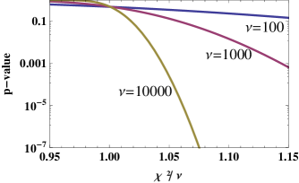
Figure 1: Colour online: The p-value as a function of the reduced $\chi^{2}$ for different number of degrees of freedom $\nu=100,1000,10000$.

In hadronic physics, at least at low energies, there is a bunch of field theoretical conditions involving relativity, analiticity, unitarity, crossing and chiral symmetry that apply only to the strong interactions, which are short range. Are these conditions powerful enough to discard some reported scattering data in favour of other scattering data ?. A practical problem is related to the presence of long range effects such as Coulomb interaction, vacuum polarization or magnetic interactions, etc. which are hard to implement, say, within dispersion relations, but influence peripheral scattering. The standard approach is to first “clean” the database by other method and then “remove” the long range effects from the data, so that the theory can then be tested. A particularly revealing example is the recent $np$ and $pp$ analysis of scattering data, where the so called coarse grained potential model has been found to provide the largest mutually $3\sigma$ self-consistent Granada-2013 database at about pion production threshold [5]. One important consequence of this database is that paves the road for theoretical tests such as ChPT [6]. In fact, it has recently been shown [7] that ChPT for NN at N5LO allows quite accurately to describe this database, in fact, outperforming the previously popular potentials which had been considered “high quality” .

3 Invariant momentum approach

From a fundamental point of view the relativistic two body problem is best analyzed in terms of the honorable Bethe-Salpeter equation (BSE) [9], where exact solutions and numerical methods have been studied exhaustively over the years (for a review on the relativistic few body problem see e.g. [10], and references therein). This is a good approach as long as the input of the equation, the two particle irreducible (2PI) 4-point funtion is known exactly. However, one must point out that the 2PI Green function is mostly accessible only within perturbation theory. The problem with this approach is that for the usual hadronic couplings the ultraviolet structure of the 2PI 4-point function becomes increasingly divergent and thus the scattering problem becomes ill defined. For instance, numerous studies have been concerned over the years about minimal sets of diagrams which implement compelling properties. However, in order to compare to experiment, the 2PI kernel is ultimately phenomenologically parameterized and interpreted from a fit to experimental data. Therefore many, in principle different, 3D reductions are in fact equivalent from a perturbative point of view [11].

Besides, there is the problem of off-shellness; a perturbative evaluation of the amplitude yields unique results only when all variables are taken to be on-shell. Off-shell extrapolations are in a sense arbitrary and also depend on the field parameterization [12]. A fairly old but unknown study [13] analyzes the interplay between on-shell and off-shell in terms of a non-linear dispersion relation (see e.g. Ref. [14]). Under those conditions it is far more useful to use a much simpler approach such as the mass-invariant method [15] which is based on rewritting the problem and matching the potential perturbatively as has been proposed e.g. in Refs. [12]. For the case of unequal masses the mass-invariant scheme generates a complicated equation, but we can instead proceed in a CM-momentum invariant approach, namely

$$\left[-\nabla^{2}+U(\vec{r})\right]\Psi=p_{\rm CM}^{2}\Psi\,,$$ (1)

where for $W=\sqrt{s}=\sqrt{p^{2}+M^{2}}+\sqrt{p^{2}+m^{2}}$ (we drop the subscript CM from now)

$$p^{2}=\frac{(m-M-W)(m+M-W)(m-M+W)(m+M+W)}{4W^{2}}\,.$$ (2)

The upshot is that for all purposes we can use a Schrödinger type equation where the non-relativistic CM momentum is promoted to a relativistic one as given by the previous equation where the interaction $U(\vec{r})$ can be determined by matching to ChPT at long distances, $r>r_{c}$ and the coarse graining principle can be applied to small distances $r<r_{c}$ with $r_{c}$ a suitable short distance cut-off.

4 Elastic scattering and finite resolution

For two particle scattering the spatial resolution in the relative cooredinate is fixed by the shortest relative de Broglie wavelength, which is given by

$$\Delta r=\frac{\hbar}{p}=\lambda_{\rm min}/(2\pi)\,.$$ (3)

Quantum field theory requires particle exchange to account for interactions which for hadrons have a maximal range about the Compton wavelength of the lightest hadron and are ${\cal O}(e^{-r/\lambda_{C}})$ with $r$ the relative distance between hadrons. That means $\lambda_{C}=\hbar/m_{\pi}c=1.4\,{\rm fm}$ for One Pion Exchange (OPE) as it is the case for $NN$ interactions and $\lambda_{C}=\hbar/2m_{\pi}c=0.7\,{\rm fm}$ for Two Pion Exchange (TPE) which corresponds to $\pi N$ and $\pi\pi$ interactions. Because of the exponential fall-off we take the range numerically $a\sim 2\lambda_{C}$.

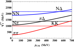
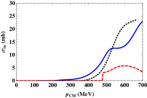
Figure 2: Colour online: (left panel) The CM energy as a function of the CM momentum for $\pi\pi$ (solid,red) , $\pi N$ (solid,black) and $NN$ (solid,blue). We also plot the corresponding thresholds at $K\bar{K}$, $\pi\Delta$ and $N\Delta$ where the inelastic cross (right panel) section increases substantially (we take $\pi^{0}\pi^{0}$, $\pi^{+}p$ and $pp$ respectively.

In our presentation we will restrict to the case of elastic $\pi\pi$, $\pi N$ and $NN$ interactions which definitely set an upper limit for the CM energy. Inelastic thresholds are marked by pion production processes, such as $\pi\pi\to\pi\pi\pi\pi$, $\pi N\to\pi\pi N$ or $NN\to NN\pi$, but they generate small contributions to the inelastic cross section so that their influence on the dominant elastic process can be neglected. Actually, the inelastic cross section experiences a rapid change when $\pi\pi\to K\bar{K}$, $\pi N\to\pi\Delta$ and $NN\to N\Delta$ corresponding to $\sqrt{s}=2m_{K},m_{\pi}+M_{\Delta},M_{N}+M_{\Delta}$ respectively.

In Fig. 2 we depict the CM energy as a function of the CM momentum as well as the location of the thresholds where the inelastic cross section undergoes a sudden rise. As we see this happens in the CM momentum range of about a similar value $p_{CM}\sim 350-550$ which corresponds to a resolution $\Delta r=\hbar/p_{\rm CM}\sim 0.3-0.6\,{\rm fm}$. As we see, they lie well at higher energies than the single and double production thresholds. The reason why the inelasticity is so tiny is likely to be found in chiral symmetry and the fact that the pion couples derivatively, which suppresses the production amplitude by extra powers of momentum. In any case, these higher thresholds are the natural limit for a purely elastic scattering description. Going to higher energies is possible but it requires implementing energy dependence into the potential.

5 Anatomy of hadronic interactions

5.1 Effective elementarity

Hadrons have a finite size, which only becomes visible when the probing wavelength is comparable. Longer wavelengths make the hadron look as elementary and pointlike particles. This feature can be best appreciated by analyzing the electromagnetic (em) interaction of charged particles such as, e.g., $\pi^{+}\pi^{+}$, $\pi^{+}p$ and $pp$. This can be readily estimated by using

$$V_{AB}^{\rm em}(r)=\int d^{3}x_{1}\int d^{3}x_{2}\frac{\rho_{A}(\vec{x}_{1})\rho_{B}(\vec{x}_{2})}{|\vec{x}_{1}-\vec{x}_{2}-\vec{r}|}\,,$$ (4)

where $\rho_{A}(\vec{x})$ and $\rho_{B}(\vec{x})$ are the charge densities corresponding to hadrons A and B respectively. Using the electric form factors in the Breit frame

$$eF_{i}(\vec{q}) = \int d^{3}x\rho_{A,B}(\vec{x})e^{i\vec{q}\cdot\vec{x}}\,,$$ (5)

with $i=A,B$, we obtain

$$V_{AB}^{\rm em}(r)=e^{2}\int\frac{d^{3}q}{(2\pi)^{3}}\frac{4\pi}{\vec{q}^{2}}F_{A}(\vec{q})F_{B}(\vec{q})e^{i\vec{q}\cdot\vec{r}}\sim\frac{q_{A}q_{B}}{r}\qquad r\geq r_{e}\,.$$ (6)

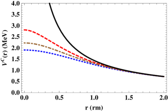
Figure 3: Colour online: Electromagnetic potentials for pointlike charge one particles (Solid,Black) and finite size particles , $\pi^{+}\pi^{+}$ (Red,dashed) , $\pi^{+}p$ (Brown, dotted-dashed) and $pp$ (Blue,dotted) as a function of the distance.

As we see by looking at Fig. 3, the elementarity radius $r_{e}$ falls in the range $\sim 1.5\,{\rm fm}$. This suggests that in order be entitled to ignore the finite hadron size, one should take the cut-off distance to satisfy $r_{c}\geq r_{e}\sim 1.5\,{\rm fm}$ . Of course, this effective elementarity feature occurs also for the strong interaction, and we will assume that the corresponding elementarity radius coincides with the one found in the em case.

5.2 Impact parameter

Due to angular momentum conservation one can use a partial wave expansion for the quantum mechanical scattering amplitude, which in the spinless case reads

$$f(\theta,W)=\sum_{J=0}^{\infty}(2J+1)P_{J}(\cos\theta)\frac{e^{i\delta_{J}}\sin\delta_{J}}{p}\,.$$ (7)

The standard semiclassical argument yields the relation

$$J+\frac{1}{2}=pb\,,$$ (8)

between the impact parameter $b$ and the angular momentum $J$ The no-scattering situation corresponds to $b\geq a$ with $a$ the range of the interaction, so that the partial wave expansion is effectively truncated for a maximum angular momentum $J_{\rm max}+1/2\sim pa$. Operationally, one may take a more refined condition where the phase-shift becomes zero within experimental uncertainties. Actually, this is a model independent way of estimating from a data analysis the finite range of the interaction $a$.

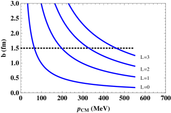
Figure 4: Colour online: The impact parameter as a function of the CM momentum for different partial waves with angular momenta $L=0,1,2,3$ (solid,blue). The (black,dotted) line indicates the critical radius marking the range of the interaction.

In Fig. 4 we show the dependence of the impact parameter on the CM momentum for the lowest partial waves with angular momentum $L=0,1,2,3$ assuming for simplicity $r_{c}=1.5\,{\rm fm}$. For instance, if we have $p_{\rm CM}\leq 300\,{\rm MeV}$ only S- and P-waves probe the interaction region . For a given partial wave the idea of coarse graining is illustrated in Fig. 5 for a maximal CM momentum of $p_{\rm max}=400\,{\rm MeV}$.

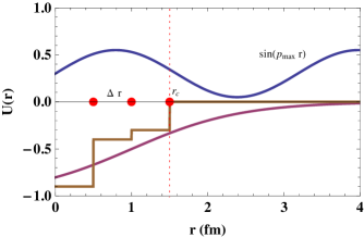
Figure 5: Colour online: An illustration of the coarse graining idea for a maximal CM momentum $p_{\rm max}=400\,{\rm MeV}$ which corresponds to a wavelength $\lambda_{\rm min}=3$ and hence $\Delta r=0.5\,{\rm fm}$

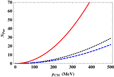
Figure 6: Colour online: (Left panel) Allowed independent parameters (shaded area) based on coarse graining the interaction below $r_{c}=1.5\,{\rm rm}$. (Right panel) The estimated number of independent parameters as a function of the CM momentum for $\pi\pi$ (dashed,blue) , $\pi N$ (dotted,black) and $NN$ (solid,red) scattering.

5.3 The number of parameters

Once we fix maximum CM momentum $p_{\rm CM,max}$ and the cut-off radius $r_{c}$ the number of parameters $N_{\rm Par}$ can be easily calculated as follows. For a central potential $U(r)$ one has a tower of angular momentum states $L=0,1,2,\cdots$. The maximal angular momentum corresponds to

$$L_{\rm max}+\frac{1}{2}=pr_{c}$$ (9)

If we take the $L=0$ state, we have the grid points

$$\Delta r=\hbar/p_{\rm CM,max}\to r_{n}=n\Delta r\,.$$ (10)

The idea is to use $U_{n}\equiv U(r_{n})$ as fitting parameter. According to the previous discussion, the number of points would be $(r_{c}/\Delta r)\times L_{\rm max}\sim(p_{\rm CM,max}r_{c})^{2}$. However, the actual number is smaller since for $L\geq 1$ some of the points located at $r_{n}$ fall well below the centrifugal barrier, and correspond to the classicaly forbidden region, thus their contribution is suppressed. Taking into account both spin and isospin degrees of freedom the following estimate can be obtained as [17]

$$N_{\rm par}=N_{S}N_{I}\sum_{L=0}^{L_{\rm max}}\sum_{n}\theta\left[p^{2}-\frac{L(L+1)}{r_{n}^{2}}\right]\sim\frac{1}{2}(pr_{c})^{2}N_{S}N_{I}\,,$$ (11)

where $N_{S}$ and $N_{I}$ the number of spin and isospin channels respectively. The number of independent parameters is plotted in Fig. 6 as a function of the maximal CM momentum and for $r_{c}=1.5\,{\rm fm}$. Remarkably, for the $NN$ case, $N_{\rm Par}\sim 50$ which explains the traditional number of fitting parameters for “high quality” NN analyses over the years [18]. For $\pi\pi$ scattering below $K\bar{K}$ threshold, one needs $N_{\rm Par}\sim 9=3\times(S_{00})+3\times(S_{20})+3\times(P_{11})$ [19]. For $\pi N$ scattering with $\sqrt{s}\leq m_{\pi}+M_{\Delta}=1.38\,{\rm GeV}$ the total number of fitting parameters would be about $18=3\times(S_{11}+S_{31})+3\times(P_{11}+P_{31}+P_{13}+P_{33})$ [20].

5.4 Complete potential

The current attempts to verify the suitability of the coarse graining approach have proved successful so far. The delta-shells approach is by far the simplest scheme where the coarse graining of the interaction can be implemented. The complete fitting potential (delta-shells)

$$U(r)=\underbrace{\left\{\sum_{i}\Delta rU(r_{i})\delta(r-r_{i})\right\}}_{\rm Short(Coarse\,grained)}\theta(r_{e}-r)+\underbrace{U_{\rm ChPT}(r)}_{\rm Long(Particle\,exchange)}\theta(r-r_{e})\,.$$ (12)

Here $U_{\rm ChPT}(r)$ is the chiral part which can be obtained from the corresponding Feynman diagrams having a $t$-channel discontinuity [19]. For $r_{c}\sim 1.5\,{\rm fm}$ one takes $U_{\rm QFT}(r)=U_{\rm 1\pi}(r)+U_{\rm 2\pi}(r)$ ( $1\pi$ and $2\pi$ exchange) for NN [21, 22] and $U_{\rm QFT}(r)=U_{\rm 2\pi}(r)$ ($2\pi$ exchange) for $\pi\pi$ [19] and $\pi N$ [20].

6 Closing remarks

As we have discussed, for a maximal CM energy the number of independent parameters characterizing the phenomenological interaction is finite and in principle independent on the precision of the experimental data. A this point it is pertinent to compare with ChPT. A simple way to estimate how many parameters are needed, proceeds by analysing the scattering amplitude close to threshold. In the case of $\pi\pi$ scattering and assuming isospin invariance, the scattering amplitudes for $I=0,1,2$ depend on a unique function $A(s,t,u)$ which for on-shell particles becomes $F(s,t)$. In the chiral counting and going to small energies one has $s,t,m_{\pi}^{2}={\cal O}(p^{2})$ we expand

$$F(s,t,m_{\pi}^{2})=\sum_{k,l=0}\frac{c_{kl}^{N}}{f^{N}}s^{k}t^{l}(m_{\pi}^{2})^{N-k-l}\,,$$ (13)

with $f$ the pion weak decay constant. The number of independent parameters, $c_{kl}^{N}$, corresponds to the number of partitions of the order $N$ by three positive integers which is $(N+1)(N+2)/2=3,6,10,15,21\dots$ for $N=1,2,3,4,5,\dots$. Thus, ChPT has a finite applicability range with an increasing number of parameters which improve the accuracy at a given finite order. Similar features apply to $NN$ [18] and $\pi N$ [20]. Thus, the validation of the theory is related to the accuracy of the data. Standard $\chi^{2}$ minimization allows to determine the LEC’s

$$\chi_{\rm min}^{2}=\min_{c_{1},c_{2},\dots}\chi^{2}(c_{1},c_{2},\dots)=\sum_{i=1}^{N_{\rm Dat}}\left[\frac{{\cal O}_{i}^{\th}(c_{1},c_{2},\dots)-{\cal O}_{i}^{\rm exp}}{\Delta{\cal O}_{i}^{\rm exp}}\right]^{2}$$ (14)

The problem is that we need $N_{\rm Par}\to\infty$ when $\Delta{\cal O}^{\rm exp}\to 0$ or $N_{\rm Dat}\to\infty$ . In contrast, in the coarse graining approach we expect $N_{\rm Par}\sim(pr_{c})^{2}$ regardless on $\Delta{\cal O}^{\rm exp}$. Whether or not the coarse graining approach qualifies as expected for fitting and selecting, for instance, $\pi N$ scattering data remains to be seen.

References

- [1] S. Weinberg, Phenomenological Lagrangians, Physica A96 (1979) 327–340.
- [2] S. Weinberg, Effective field theory, past and future, Int. J. Mod. Phys. A31 (2016) 1630007.
- [3] E. Ruiz Arriola, J. E. Amaro and R. Navarro Pérez, Fitting and selecting scattering data, PoS Hadron2017 (2018) 134, [1711.11338].
- [4] R. Navarro Pérez, E. Ruiz Arriola and J. Ruiz de Elvira, Self-consistent statistical error analysis of scattering, Phys. Rev. D91 (2015) 074014, [1502.03361].
- [5] R. Navarro Pérez, J. E. Amaro and E. Ruiz Arriola, Coarse-grained potential analysis of neutron-proton and proton-proton scattering below the pion production threshold, Phys. Rev. C88 (2013) 064002, [1310.2536].
- [6] E. Ruiz Arriola, J. E. Amaro and R. Navarro Pérez, The falsification of Chiral Nuclear Forces, EPJ Web Conf. 137 (2017) 09006, [1611.02607].
- [7] P. Reinert, H. Krebs and E. Epelbaum, Semilocal momentum-space regularized chiral two-nucleon potentials up to fifth order, Eur. Phys. J. A54 (2018) 86, [1711.08821].
- [8] D. R. Entem, R. Machleidt and Y. Nosyk, High-quality two-nucleon potentials up to fifth order of the chiral expansion, Phys. Rev. C96 (2017) 024004, [1703.05454].
- [9] E. E. Salpeter and H. A. Bethe, A Relativistic equation for bound state problems, Phys. Rev. 84 (1951) 1232–1242.
- [10] J. Carbonell, B. Desplanques, V. A. Karmanov and J. F. Mathiot, Explicitly covariant light front dynamics and relativistic few body systems, Phys. Rept. 300 (1998) 215–347, [nucl-th/9804029].
- [11] J. Nieves and E. Ruiz Arriola, Bethe-Salpeter approach for unitarized chiral perturbation theory, Nucl. Phys. A679 .
- [12] E. Ruiz Arriola, Some Three-body force cancellations in Chiral Lagrangians, 1606.07535.
- [13] J. Namyslowski, Relativistic, 3-dimensional, 2-body integral equations. on-shell and off-shell formalisms, Physical Review 160 (1967) 1522.
- [14] M. F. M. Lutz, E. E. Kolomeitsev and C. L. Korpa, Spectral representation for u- and t-channel exchange processes in a partial-wave decomposition, Phys. Rev. D92 (2015) 016003, [1506.02375].
- [15] T. W. Allen, G. L. Payne and W. N. Polyzou, Comparison of relativistic nucleon-nucleon interactions, Phys. Rev. C62 (2000) 054002, [nucl-th/0005062].
- [16] I. R. Simo, J. E. Amaro, E. Ruiz Arriola and R. Navarro Perez, Low energy peripheral scaling in nucleon-nucleon scattering and uncertainty quantification, J. Phys. G45 (2018) 035107, [1705.06522].
- [17] P. Fernandez-Soler and E. Ruiz Arriola, Coarse graining of NN inelastic interactions up to 3 GeV: Repulsive versus structural core, Phys. Rev. C96 (2017) 014004, [1705.06093].
- [18] R. Navarro Perez, J. E. Amaro and E. Ruiz Arriola, Partial Wave Analysis of Chiral NN Interactions, Few Body Syst. 55 (2014) 983–987, [1310.8167].
- [19] J. Ruiz de Elvira and E. Ruiz Arriola, Coarse graining scattering, Eur. Phys. J. C78 (2018) 878, [1807.10837].
- [20] J. M. Alarcón, J. Ruiz de Elvira and E. Ruiz Arriola, Coarse graining scattering, In preparation .
- [21] R. Navarro Pérez, J. E. Amaro and E. Ruiz Arriola, Coarse grained NN potential with Chiral Two Pion Exchange, Phys. Rev. C89 (2014) 024004, [1310.6972].
- [22] R. Navarro Pérez, J. E. Amaro and E. Ruiz Arriola, Low energy chiral two pion exchange potential with statistical uncertainties, Phys. Rev. C91 (2015) 054002, [1411.1212].