Nonfactorizable QCD Effects in Higgs Boson Production via Vector Boson Fusion

Abstract

We discuss nonfactorizable QCD corrections to Higgs boson production in vector boson fusion at the Large Hadron Collider. We point out that these corrections can be computed in the eikonal approximation retaining all the terms that are not suppressed by the ratio of the transverse momenta of the tagging jets to the total center-of-mass energy. Our analysis shows that in certain kinematic distributions the nonfactorizable corrections can be as large as a percent making them quite comparable to their factorizable counter-parts.

Vector boson fusion (VBF) is one of the two key channels for Higgs boson production at the Large Hadron Collider (LHC) Khachatryan:2015bnx ; Aaboud:2018gay . Studies of Higgs boson properties in this process require accurate theoretical prediction for its cross section and kinematic distributions. Radiative corrections, both QCD and electroweak, are important for the reliable description of these processes. Current understanding of QCD corrections to the VBF Higgs boson production is highly advanced: following the original calculation of the next-to-leading (NLO) corrections Figy:2003nv , both the next-to-next-to-leading (NNLO) Bolzoni:2010xr ; Cacciari:2015jma ; Cruz-Martinez:2018rod and the next-to-next-to-next-to-leading (N³LO) Dreyer:2016oyx corrections were computed in the so-called structure function approximation Han:1992hr . The electroweak corrections to VBF were computed in Ref. cicco . Other interesting effects such as loop-induced interference between Higgs production in gluon fusion and in vector boson fusion, and the gluon-initiated VBF Higgs production were studied in Refs. jeppe ; rob , respectively.

The structure function approximation – the centerpiece of the current studies of QCD effects in VBF – neglects interactions between incoming QCD partons and retains QCD effects confined to a single fermion line. There are good reasons for doing this. Indeed, at NLO the gluon exchanges between different quark lines do not change the VBF cross section as a consequence of color conservation. At NNLO, two gluons exchanged between two fermion lines can be in a color-singlet state and for this reason do contribute to the VBF cross section. Such nonfactorizable corrections, however, are necessarily color-suppressed, making it plausible that they are small. This argument was used as the justification for computing higher-order QCD corrections to VBF Higgs boson production in the structure function approximation Bolzoni:2010xr .

However, it is interesting to ask just for how long does it make sense to improve the precision on the factorizable contributions while ignoring the nonfactorizable ones. This question appears to be quite relevant since computations of factorizable contributions have advanced to very high orders in perturbative QCD Dreyer:2016oyx . Answering this question is difficult since not much is known about nonfactorizable corrections beyond their color suppression. As we already mentioned, these corrections do not contribute at NLO while at NNLO they require two-loop five-point functions that depend on many kinematic variables and the masses of vector bosons and the Higgs boson. Thus, the technical complexity of perturbative computations required to obtain the two-loop nonfactorizable contribution appears to be overwhelming to expect significant advances in the foreseeable future. An estimate of nonfactorizable corrections that makes use of QCD dynamics and in this sense goes beyond the color-suppression argument is highly desirable, in our opinion.

In this Letter we will show that it is possible and in fact rather simple to compute the dominant contribution to nonfactorizable corrections, making use of the particular kinematics of the VBF process. Indeed, this process is identified by the presence of two forward tagging jets whose transverse momenta are small compared to their energies. Thus, we can try to compute the nonfactorizable corrections in an approximation where we only retain contributions that are leading in $p_{j,\perp}/\sqrt{s}$, where $p_{j,\perp}$ is a transverse momentum of a tagging jet, and $s$ is the center-of-mass energy squared of the colliding partons. Since in the VBF process $\sqrt{s}\;\hbox to0.0pt{\lower 3.5pt\hbox{$\mathchar 0\relax\sim$}\hss}\raise 1.0pt\hbox{$>$}\;600~{}{\rm GeV}$ and $p_{j,\perp}\sim 100~{}{\rm GeV}$ Khachatryan:2015bnx ; Aaboud:2018gay this approximation is justified in large part of the phase space.

It is well known that the computation of cross sections at leading power in the small ratio $p_{\perp,j}/\sqrt{s}$, can be performed within the eikonal approximation for the colliding particles Cheng:1970jk ; Chang:1969by ; Lipatov:1976zz . To explain this approximation, we consider a collision of two quarks that leads to the production of the Higgs boson in VBF

$$q_{1}(p_{1})+q_{2}(p_{2})\to q_{1}(p_{3})+q_{2}(p_{4})+H(p_{5}).$$

The leading order contribution to this process is shown in Fig. 1(a). The eikonal approximation separates dynamics in the plane spanned by the two four-momenta of the incoming quarks $p_{1,2}$ from dynamics in the plane that is transversal to it. We will refer to a component of a four-vector $k^{\mu}$ in the transversal plane as $k_{\perp}^{\mu}$ or $k$. We choose the reference frame in such a way that $p_{1}$ and $p_{2}$ have only a single light-cone component $p^{-}_{1}$ and $p^{+}_{2}$, respectively. Then in the eikonal approximation a gauge boson coupling to the quark line with momentum $p_{1}$ ($p_{2}$) is obtained by replacing the corresponding current $j^{\mu}$ with its light-cone component $j^{-}$ ($j^{+}$) while the quark propagators are replaced as follows

$$\begin{split}&{1\over\not{p}_{1,2}+\not{k}+i\epsilon}\to{\gamma^{\pm}\over 2k^{\pm}+i\epsilon}\,,\end{split}$$ (1)

where $\gamma^{\pm}$ are the light-cone components of the Dirac $\gamma$-matrices.

In the VBF process Higgs bosons are produced at central rapidities so that they are well-separated from the tagging jets. This ensures that momentum transfers $q_{3}=p_{3}-p_{1}$ and $q_{4}=p_{4}-p_{2}$ mostly have transverse components ${\mbox{\boldmath$q$}_{3,4}}$ while their light-cone component are suppressed by $p_{{3,4},\perp}/\sqrt{s}$. Thus, the Higgs boson emission does not spoil the applicability of the eikonal approximation.

(a)	(b)	(c)

Figure 1: The Feynman diagrams for the Higgs boson production in VBF: (a) the Born amplitude, (b, c) the one-loop nonfactorizable QCD corrections. The solid, dashed, wavy and loopy lines stay for quark, Higgs, vector boson and gluon fields, respectively.

We continue with the discussion of the nonfactorizable QCD corrections. In the one-loop approximation the relevant diagrams are shown in Fig. 1(b,c). Since electroweak vector bosons do not carry color, the one-loop contribution to the cross section vanishes at NLO by color conservation. Nevertheless, the square of the one-loop amplitude contributes to the NNLO cross section along with the generic two-loop nonfactorizable corrections. In both cases the two gluons connecting the different quark lines must be in a color-singlet configuration. Thus we can compute the corrections by replacing gluons by abelian gauge bosons with the effective coupling $\tilde{\alpha}_{s}=\left({N_{c}^{2}-1\over 4N_{c}^{2}}\right)^{1/2}\!\!\!\alpha_{s}$, where $N_{c}=3$ and the prefactor arises from averaging over colors. Considering the sum of the planar and non-planar diagrams in Figs. 1(b,c), we find that the eikonal quark propagators add up to $1/(2k^{\pm}+i\epsilon)-c.c.=-i\pi\delta(k^{\pm})$. Hence, when the two diagrams are combined, the virtual quark propagators are replaced by $\delta(k^{+})$ and $\delta(k^{-})$ and the light-cone dynamics decouples. Thus the computation of the nonfactorizable one-loop contribution is reduced to the analysis of the effective Feynman diagram shown in Fig. 2(a) in the two-dimensional transversal space. In the eikonal approximation QCD corrections are diagonal in the chiral basis. This implies that (for a given type of electroweak gauge bosons that fuse into the Higgs) the Born amplitude ${\cal M}^{(0)}$ factors out. Hence, the expression for the one-loop amplitude can be written as follows

$$\begin{split}&{\cal M}^{(1)}=i\tilde{\alpha}_{s}\chi^{(1)}({\mbox{\boldmath$q$}}_{3},{\mbox{\boldmath$q$}}_{4}){\cal M}^{(0)}\,,\end{split}$$ (2)

with

$$\begin{split}&\chi^{(1)}({\mbox{\boldmath$q$}}_{3},{\mbox{\boldmath$q$}}_{4})=\frac{1}{\pi}\int\frac{{\rm d}^{2}{\mbox{\boldmath$k$}}}{{\mbox{\boldmath$k$}}^{2}+\lambda^{2}}\\ &\times\frac{{\mbox{\boldmath$q$}}_{3}^{2}+M_{V}^{2}}{({\mbox{\boldmath$k$}}-{\mbox{\boldmath$q$}}_{3})^{2}+M_{V}^{2}}\frac{{\mbox{\boldmath$q$}}_{4}^{2}+M_{V}^{2}}{({\mbox{\boldmath$k$}}+{\mbox{\boldmath$q$}}_{4})^{2}+M_{V}^{2}}\,,\end{split}$$ (3)

where $M_{V}=M_{Z,W}$ is an electroweak boson mass. We note that the function $\chi^{(1)}$ is ultraviolet-finite but infrared-divergent. To regulate the infrared divergence, we introduced an auxiliary gluon mass $\lambda$. Moreover, the function $\chi^{(1)}$ is explicitly real, so that the entire one-loop correction is imaginary. This is yet another reason, in addition to color conservation, that leads to vanishing interference between the one-loop amplitude computed in the eikonal approximation and the leading order amplitude.

(a)	(b)

Figure 2: One- and two-loop transversal space Feynman diagrams.

At two loops the structure of the corrections is similar. In the color-singlet configuration the gluon vertices commute and the factorization property of the eikonal approximation Sudakov:1954sw can be applied. As a result the sum over all the permutations of the gluon and vector-boson vertices reduces to the effective transversal space diagram in Fig. 2(b) Cheng:1970jk . The corresponding expression for the amplitude reads

$$\begin{split}&{\cal M}^{(2)}=-{\tilde{\alpha}^{2}_{s}\over 2!}\chi^{(2)}({\mbox{\boldmath$q$}}_{3},{\mbox{\boldmath$q$}}_{4}){\cal M}^{(0)}\,,\end{split}$$ (4)

where $1/2!$ factor results from the symmetrization of two identical gluons and

$$\begin{split}&\chi^{(2)}({\mbox{\boldmath$q$}}_{3},{\mbox{\boldmath$q$}}_{4})=\frac{1}{\pi^{2}}\int\left(\prod\limits_{i=1}^{2}\frac{{\rm d}^{2}{\mbox{\boldmath$k$}}_{i}}{{\mbox{\boldmath$k$}}_{i}^{2}+\lambda^{2}}\right)\\ &\times\frac{{\mbox{\boldmath$q$}}_{3}^{2}+M_{V}^{2}}{({\mbox{\boldmath$k$}}_{1}+{\mbox{\boldmath$k$}}_{2}-{\mbox{\boldmath$q$}}_{3})^{2}+M_{V}^{2}}\frac{{\mbox{\boldmath$q$}}_{4}^{2}+M_{V}^{2}}{({\mbox{\boldmath$k$}}_{1}+{\mbox{\boldmath$k$}}_{2}+{\mbox{\boldmath$q$}}_{4})^{2}+M_{V}^{2}}\,.\end{split}$$ (5)

Squaring the sum of tree-, one- and two-loop contributions to the scattering amplitude, we obtain the NNLO QCD correction to the cross section due to nonfactorizable contributions

$${\rm d}\sigma^{\rm NNLO}_{\rm nf} = \left({N_{c}^{2}-1\over 4N_{c}^{2}}\right)\alpha_{s}^{2}\,\chi_{\rm nf}\,{\rm d}\sigma^{\rm LO}\,.$$ (6)

In Eq.(6) ${\rm d}\sigma^{\rm LO}$ is the leading-order differential cross section for VBF and

$$\chi_{\rm nf}({\mbox{\boldmath$q$}_{3}},{\mbox{\boldmath$q$}_{4}})=\left[\chi^{(1)}({\mbox{\boldmath$q$}_{3}},{\mbox{\boldmath$q$}_{4}})\right]^{2}-\chi^{(2)}({\mbox{\boldmath$q$}_{3}},{\mbox{\boldmath$q$}_{4}})\,$$ (7)

is the nonfactorizable correction.

The nonfactorizable correction has peculiar properties. It is independent of the vector boson couplings to quarks and to the Higgs boson; these couplings are accommodated in the leading order cross section in Eq. (6). In the large-$N_{c}$ limit the color factor in Eq. (6) remains finite while for the factorizable corrections it grows as $N_{c}^{2}$ providing the color suppression of the nonfactorizable contribution. Finally, the two terms in Eq. (7) are separately infrared divergent. These divergences, however, are not related to the usual (nonfactorizable) real soft gluon emissions that, in fact, are suppressed as $p_{\perp}/\sqrt{s}$ and, therefore, do not contribute to the VBF cross section at leading power. The infra-red divergencies in non-factorizable corrections originate from the exchange of static Glauber gluons Glauber propagating in the transversal space. It is well known that when abelian gauge bosons are exchanged, the amplitudes acquire a factor $e^{i\phi}$ where $\phi$ is the infrared-divergent Glauber phase $\phi=-\tilde{\alpha}_{s}\ln\lambda^{2}$ Cheng:1970jk . This phase factor disappears in the cross section, which means that the infrared-divergent parts of the first and the second term in Eq. (7) must cancel each other.

To show this cancellation explicitly, we consider the $\lambda\to 0$ limit, extract the infrared singularities from the two functions $\chi^{(1,2)}$ and write them as follows

$$\begin{split}&\chi^{(1)}=-\ln\left(\frac{\lambda^{2}}{M_{V}^{2}}\right)+f^{(1)}\,,\\ &\chi^{(2)}=\ln^{2}\left(\frac{\lambda^{2}}{M_{V}^{2}}\right)-2\ln\left(\frac{\lambda^{2}}{M_{V}^{2}}\right)f^{(1)}+f^{(2)}\,.\end{split}$$ (8)

The functions $f^{(1),(2)}$ read

$$f^{(1)} = \int\limits_{0}^{1}{\rm d}x\frac{\Delta_{3}\Delta_{4}}{r^{2}_{12}}\left[\ln\left(\frac{r_{12}^{2}}{r_{2}M_{V}^{2}}\right)+\frac{r_{1}-r_{2}}{r_{2}}\right],$$

$$f^{(2)} = \int\limits_{0}^{1}{\rm d}x\frac{\Delta_{3}\Delta_{4}}{r_{12}^{2}}\left[\left(\ln\left(\frac{r_{12}^{2}}{r_{2}M_{V}^{2}}\right)+\frac{r_{1}-r_{2}}{r_{2}}\right)^{2}\right.$$

$$\left.-\ln^{2}\left(\frac{r_{12}}{r_{2}}\right)-\frac{2r_{12}}{r_{2}}\ln\left(\frac{r_{12}}{r_{2}}\right)-2\,{\rm Li}_{2}\left({r_{1}\over r_{12}}\right)\right.$$

$$\left.-\left(\frac{r_{1}-r_{2}}{r_{2}}\right)^{2}+\frac{\pi^{2}}{3}\right],$$

where we used the notations

$$\begin{split}&r_{1}={\mbox{\boldmath$q$}}_{3}^{2}\,x+{\mbox{\boldmath$q$}}_{4}^{2}\,(1-x)-{\mbox{\boldmath$q$}}_{H}^{2}\,x(1-x)\,,\\ &r_{2}={\mbox{\boldmath$q$}}_{H}^{2}\,x(1-x)+M_{V}^{2}\,,\\ &r_{12}=r_{1}+r_{2}\,,\\ &\Delta_{i}={\mbox{\boldmath$q$}}_{i}^{2}+M_{V}^{2}\,.\end{split}$$ (10)

In Eq.(10) ${\mbox{\boldmath$q$}}_{H}=-{\mbox{\boldmath$q$}}_{4}-{\mbox{\boldmath$q$}}_{3}$ is the Higgs boson transverse momentum. This result can be obtained by using the Feynman parameter representation for one- and two-loop two-dimensional triangle diagrams corresponding to the functions $\chi^{(1)}$ and $\chi^{(2)}$ respectively.

We note that it should be possible to compute the two functions analytically. However, the one-dimensional integral representations in Eqs. (Nonfactorizable QCD Effects in Higgs Boson Production via Vector Boson Fusion,10) are perfectly suitable for the numerical evaluation of the nonfactorizable corrections so that we decided not to pursue the analytic calculation further.

Using representations Eq. (8) in Eq. (7), we obtain the finite result

$$\chi_{\rm nf}({\mbox{\boldmath$q$}_{3}},{\mbox{\boldmath$q$}_{4}})=[f^{(1)}({\mbox{\boldmath$q$}_{3}},{\mbox{\boldmath$q$}_{4}})]^{2}-f^{(2)}({\mbox{\boldmath$q$}_{3}},{\mbox{\boldmath$q$}_{4}})\,,$$ (11)

for the two-loop nonfactorizable correction to the VBF cross section. It can be used for the numerical evaluation of the correction factor for values of the transverse momenta that are much smaller than the energy of the two colliding partons.

It is instructive to compute the function $\chi_{\rm nf}$ in a few limiting cases. The simplest case is when all the transverse momenta are small compared to the vector boson mass $|{\mbox{\boldmath$q$}}_{3,4}|\ll M_{V}$. In this limit $r_{1}=0$, $r_{2}=M_{V}^{2}$ and we find

$$\lim_{q_{3,4}\to 0}\chi_{\rm nf}=1-\frac{\pi^{2}}{3}\,.$$ (12)

Another interesting case is when the Higgs boson momentum is small ${\mbox{\boldmath$q$}}_{H}^{2}\ll M_{V}^{2},{\mbox{\boldmath$q$}}_{3,4}^{2}$. In this limit $r_{1}={\mbox{\boldmath$q$}}^{2}_{3}$, $r_{2}=M_{V}^{2}$ and we obtain

$$\begin{split}&\lim_{q_{H}\to 0}\chi_{\rm nf}=\ln^{2}\left({1+x\over x}\right)+2\,{\rm Li}_{2}\left({1\over 1+x}\right)-\frac{\pi^{2}}{3}\\ &+2\,{1+x\over x}\ln\left({1+x\over x}\right)+\left({1-x\over x}\right)^{2},\end{split}$$ (13)

with $x=M_{V}^{2}/{\mbox{\boldmath$q$}}_{3}^{2}$. In the opposite limit when the transverse momentum ${\mbox{\boldmath$q$}}_{3}$ of one of the tagging jets is small compared to ${\mbox{\boldmath$q$}}_{4}\approx{\mbox{\boldmath$q$}}_{H}$ the result reads

$$\lim_{q_{3}\to 0}\chi_{\rm nf}=\ln^{2}\left({1+x\over x}\right)+2\,{\rm Li}_{2}\left({1\over 1+x}\right)-\frac{\pi^{2}}{3}\,.$$ (14)

The coefficient of the quadratic logarithm in Eq. (13) can be read off from the infrared divergences of the one- and two-loop massless amplitudes at zero Higgs boson momentum. We have verified this coefficient by exact evaluation of the scattering amplitudes in dimensional regularization as functions of ${\mbox{\boldmath$q$}}_{3}^{2}/s$ with subsequent expansion of the result at small transverse momentum; this calculation provides a nontrivial test of the eikonal approximation used in the above analysis.

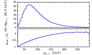
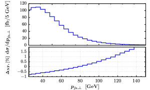
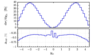
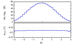
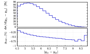
Figure 3: Differential cross sections for the transverse momentum distributions for the two leading jets, $p_{j_{1},\perp}$ and $p_{j_{2},\perp}$ and for the Higgs boson, $p_{h,\perp}$ as well as the rapidity distributions of the first jet and of the Higgs boson in VBF at the $13~{}{\rm TeV}$ LHC. We also show the rapidity difference distribution of the two tagging jets. See text for details.

One can use these asymptotic formulas to discuss characteristic features of the nonfactorizable contribution. For example, taking $\alpha_{s}\sim 0.1$, we find that the zero-momentum limit Eq. (12) implies minus one percent correction to the differential cross section Eq. (6). At the same time, the limit of the small Higgs transverse momentum Eq. (14) suggests that positive corrections as large as a few percent occur when the transverse momentum of the tagging jets exceeds $100~{}{\rm GeV}$.

It follows from the above discussion that the nonfactorizable corrections can reach a few percent in differential distributions. However, since the corrections appear with opposite signs at low and high transverse momenta, they may cancel in quantities that are inclusive with respect to kinematic features of the tagging jets.

The reason behind sizable nonfactorizable effects can be traced to their connection to the Glauber scattering phase. This connection leads to a $\pi^{2}$-enhancement of the nonfactorizable contribution characteristic to the imaginary phase, which partially overcomes the effect of the color suppression, cf. Eq. (6). Interestingly, previous attempts to estimate nonfactorizable corrections were based on the analysis of real radiation Figy:2007kv or the real part of the one-loop amplitude Bolzoni:2011cu which are insensitive to contributions of this type.

Having discussed features of the nonfactorizable contribution, we can now evaluate its impact on the VBF Higgs production cross section. We consider proton-proton collisions at the LHC with the center of mass energy $13~{}{\rm TeV}$. To select VBF events, we require that tagging jets have transverse momenta larger than $25~{}{\rm GeV}$ and their invariant mass exceeds $600~{}{\rm GeV}$. Besides that, jets’ rapidities should satisfy the conditions $y_{j_{1},j_{2}}\in[-4.5,4.5]$ and $|y_{j_{1}}-y_{j_{2}}|>4.5$. In addition, jets are required to be in opposite hemispheres. To compute the leading order cross section and the nonfactorizable corrections we adopt the following factorization and renormalization scales

$$\mu_{F}=\left[\frac{m_{h}}{2}\sqrt{\frac{m_{h}^{2}}{4}+p_{h,\perp}^{2}}\right]^{1/2},\;\;\;\mu_{R}=\sqrt{p_{j_{1},\perp}p_{j_{2},\perp}}\,.$$ (15)

Note that our choice of the factorization scale is identical to that of Ref. Cacciari:2015jma which ensures that our leading order cross sections and kinematic distributions are in agreement with that references. For numerical simulations we use the NNPDF 3.0 parton distribution function (NNPDF_nnlo_as_0118) with the default value $\alpha_{s}(m_{Z})=0.118$. Electroweak parameters are determined from the Fermi constant $G_{F}=1.16637\times 10^{-5}~{}{\rm GeV}^{-2}$ and masses of electroweak gauge bosons $M_{W}=80.398~{}{\rm GeV}$ and $M_{Z}=91.1876~{}{\rm GeV}$. We take the mass of the Higgs boson to be $m_{H}=125~{}{\rm GeV}$. Within the above setup we obtain the VBF cross section and the non-factorizable contribution at the $13~{}{\rm TeV}$ LHC

$$\sigma^{\rm LO}_{\rm VBF}=957~{}{\rm fb},\;\;\;\;\sigma^{\rm NNLO,NF}_{\rm VBF}=-3.73~{}{\rm fb}\,,$$ (16)

which implies a negative nonfactorizable correction

$$\Delta_{\rm NF}=\frac{\sigma^{\rm NNLO,NF}_{\rm VBF}}{\sigma^{\rm LO}_{\rm VBF}}\times 100\%=-0.39\%\,.$$ (17)

While the nonfactorizable correction is small, it is quite comparable to the N³LO QCD factorizable corrections computed in Ref. Dreyer:2016oyx . We note that the choice of a proper renormalization scale for the computation of nonfactorizable corrections is an interesting problem. Indeed, as follows from our computation, they appear for the first time at NNLO and so their scale dependence is not compensated. If we simply decrease (increase) the renormalization scale in Eq. (15) by a factor of two, $\Delta_{\rm NF}$ changes to $-0.5\%$ ($-0.3\%$), respectively.

The situation becomes even more interesting when we consider differential distributions. For example, in Fig. 3 the nonfactorizable QCD corrections to the transverse momentum distributions of the two jets and the Higgs boson as well as various rapidity distributions are shown. For each plot, the upper panel displays leading order distributions whereas the lower panel shows the correction $\Delta_{\rm NF}$, cf. Eq. (17), in dependence of a relevant kinematic variable. As it follows from the plots, the corrections to the jet transverse momenta distributions depend strongly on $p_{j,\perp}$ and can even exceed $1\%$ in certain cases. By contrast, the correction to Higgs transverse momentum is rather flat and, for this reason, is comparable to the correction to the VBF cross section Eq. (17). Correction to the rapidity distribution of the Higgs boson is rather flat too but some dependence on the rapidity is present in the corrections to the leading jet rapidity distribution and to the distribution in the rapidity difference of the two jets. The correction to the rapidity distribution of the second jet is similar to that of the first and we therefore do not show it separately.

We emphasize that in the numerical simulation we keep the full dependence of the leading order cross section on the kinematic variables without expanding in transverse momenta. The plots in Figs. 3 show that kinematic distributions peak at $p_{j,\perp}\approx 100$ GeV, which suggests that the leading ${\cal O}(p^{2}_{j,\perp}/s)$ power corrections to our result for $\sigma^{\rm NNLO}_{\rm nf}$ are in a few percent range and, for this reason, negligible.

Thus we have obtained analytic results for the nonfactorizable NNLO QCD corrections to the Higgs boson production in the vector boson fusion valid in the phenomenologically most interesting kinematic region where the characteristic transverse momenta are much smaller than the center-of-mass energy of the process and a rapidity gap between the Higgs boson and the tagging jets is present. The leading in $p_{j,\perp}/\sqrt{s}$ correction is related to the Glauber phase and has a natural $\pi^{2}$-enhancement along with the color suppression relative to the factorizable ones. It exhibits nontrivial dependence on the transverse momenta and rapidities of the tagging jets. Numerically, the corrections are found to be close to half of a percent although they can become as large as a percent in certain kinematic regions.

Acknowledgments. We are grateful to M. Schulze and F. Caola for providing us with the numerical code for Higgs boson production in vector boson fusion. The research of T.L. was supported by NSERC. The research of K.M. and A.P. was supported by the Deutsche Forschungsgemeinschaft (DFG, German Research Foundation) under grant 396021762 - TRR 257. The research of A.P. was supported by NSERC and Perimeter Institute for Theoretical Physics.

References

- (1) V. Khachatryan et al. [CMS Collaboration], Phys. Rev. D 92, 032008 (2015).
- (2) M. Aaboud et al. [ATLAS Collaboration], Phys. Rev. D 98, 052003 (2018).
- (3) T. Figy, C. Oleari and D. Zeppenfeld, Phys. Rev. D 68, 073005 (2003).
- (4) P. Bolzoni, F. Maltoni, S. O. Moch and M. Zaro, Phys. Rev. Lett. 105, 011801 (2010).
- (5) M. Cacciari, F. A. Dreyer, A. Karlberg, G. P. Salam and G. Zanderighi, Phys. Rev. Lett. 115, 082002 (2015); Erratum: [Phys. Rev. Lett. 120, 139901 (2018)].
- (6) J. Cruz-Martinez, T. Gehrmann, E. W. N. Glover and A. Huss, Phys. Lett. B 781, 672 (2018).
- (7) F. A. Dreyer and A. Karlberg, Phys. Rev. Lett. 117, 072001 (2016).
- (8) T. Han, G. Valencia and S. Willenbrock, Phys. Rev. Lett. 69, 3274 (1992).
- (9) M. Ciccolini, A. Denner, and S. Dittmaier, Phys. Rev. D 77, 013002 (2008).
- (10) J. R. Andersen, T. Binoth, G. Heinrich, and J. M. Smillie, JHEP 02, 057 (2008).
- (11) R. V. Harlander, J. Vollinga, and M. M. Weber, Phys. Rev. D 77, 053010 (2008).
- (12) H. Cheng and T. T. Wu, Phys. Rev. 186, 1611 (1969).
- (13) S. J. Chang and S. K. Ma, Phys. Rev. 188, 2385 (1969).
- (14) L. N. Lipatov, Sov. J. Nucl. Phys. 23, 338 (1976) [Yad. Fiz. 23, 642 (1976)].
- (15) V. V. Sudakov, Sov. Phys. JETP 3, 65 (1956) [Zh. Eksp. Teor. Fiz. 30, 87 (1956)].
- (16) R. J. Glauber, in Lectures in Theoretical Physics, edited by W. E. Brittin et al., Wiley-Interscience Inc., New York, 1959, Vol. 1.
- (17) R. K. Ellis, Z. Kunszt, K. Melnikov and G. Zanderighi, Phys. Rept. 518, 141 (2012).
- (18) T. Figy, V. Hankele and D. Zeppenfeld, JHEP 0802, 076 (2008).
- (19) P. Bolzoni, F. Maltoni, S. O. Moch and M. Zaro, Phys. Rev. D 85, 035002 (2012).