European Option Pricing of electricity under exponential functional of Lévy processes with Price-Cap principle

Martin Kegnenlezom 111University of Yaoundé I, Department of Mathematics, P.O. Box 812 Yaoundé, Cameroon. Phone: (+237)699 299 181, Email: kegnenlezom@gmail.com , Patrice Takam Soh222University of Yaoundé I, Department of Mathematics, P.O. Box 812 Yaoundé, Cameroon. Phone: (+237)699 299 181, Email: patricetakam@gmail.com , Antoine-Marie Bogso333University of Yaoundé I, Department of Mathematics, P.O. Box 812 Yaoundé, Cameroon. Phone: (+237)652 620 452, Email: ambogso@gmail.com , and
Yves Emvudu Wono 444University of Yaoundé I, Department of Mathematics, P.O. Box 812 Yaoundé, Cameroon. Phone: (+237)699 299 181, Email: yemvudu@yahoo.fr
Abstract

We propose a new model for electricity pricing based on the price cap principle. The particularity of the model is that the asset price is an exponential functional of a jump Lévy process. This model can capture both mean reversion and jumps which are observed in electricity market. It is shown that the value of an European option of this asset is the unique viscosity solution of a partial integro-differential equation (PIDE). A numerical approximation of this solution by the finite differences method is provided. The consistency, stability and convergence results of the scheme are given. Numerical simulations are performed under a smooth initial condition.

Keywords: Mean reverting jump-diffusion, option pricing, price-cap, integro-differential equation, Viscosity solution

subclass MSC: 60H10, 60H35, 65M06.

1 Introduction

In finance, options are tools that help to guard against risks. But, it is difficult to know the value of an option before the maturity date since, for this end, one has to estimate the value of the underlying in future. In the early of 1970’s, Black and Scholes [4] brought a major contribution in the evaluation of options. In the case where the underlying is a share that does not pay dividends, they construct a risk-neutral portofolio that replicates the winning profile of an option, which allows to perform the theoretical value of a European option under a closed formula. In the case of the exponential Lévy Black and Scholes model, this formula is derived from some classical results in discounting, statistics, stochastic and differential calculus. On the contrary, the valuation of options remains an open topic in the case of jump-diffusion processes due to the additional jump term that complicates calculation of option prices. This has been investigated by several authors as [5], [24] and [30]. One may distinguish two main approaches used by these authors. The first one, which relies on Fourier transform-based methods, has been introduced by Carr and Madan [9] to price and analyse European option prices. Many other authors follow the same idea to evaluate option prices. Among them one find [10], [14], [22] and [31]. The advantage of this approach relies on its high computational efficiency when the characteristic function is available. The idea here is to apply the direct discounted expectation method to evaluate the integral of the discounted payoff and risk neutral density function of the underlying process. Continuous and dicrete Fourier transforms were sucessfully applied to pricing options of three exponential Lévy models: the classical Black-Scoles model (which is a continuous exponential Lévy model), the Merton jump diffusion model (which is an exponential Lévy model with finite arrival rate of jumps), and the variance Gamma model (which is an exponential Lévy model with infinite arrival rate of jumps). However, for many other jump diffusion processes, it is not possible even by applying the Lévy-Khinchin representation to determine an analytical expression of the characteristic function. This may be due to the complexity of diffusion processes or to the fact that two or more processes are combined in the same model. Therefore one expects to evaluate option prices with rather an approximation of the characteristic function. The debate is then on the choice of a good approximation. Indeed, when the characteristic function can not be expressed explicitly, the Fourier transform method requires two levels of approximation which increases the error level in option valuation. In order to reduce approximation errors, a second approach, namely the Feynman-Kac formula-based approach, has been introduced by some authors such as [2], [6] and [11]. This approach relates the risk-neutral valuation formula to either the solution of a partial differential equation (PDE), when the model is a continuous exponential Lévy one, or to the solution of a partial integro-differential equation (PIDE) in the case of continuous Lévy process. The PDE, respectively PIDE obtained may be complex and its theoretical analysis requires new mathematical tools. However, after a numerical approximation step, the solution leads directly to the value of the option. So, we have one level of approximation. Nevertheless, theoretical analysis of the approximation (consistency, stability and convergence of the scheme) remains a challenge. Several finite difference schemes are used in the literature (see e.g. [2], [12] and [28]). Most of these works focus on pricing option when the underlying is driven by either a Lévy processes or an exponential Lévy process. Some of the main difficulties are related to the local integral term due to the fact that, on the one hand, the approximation of the risk-neutral density can often involve an infinite summation, and on the other hand, a local integral term requires a specific treatment at both theoretical and numerical levels. We may have other difficulties as the smoothness of option prices and even the degeneracy of the diffusion coefficient. To overcome such difficulties, the notion of viscosity solution was introduced by Grandall and Lions [13] for PDEs and, more generally, for PIDEs (see e.g. [2] and [6]). Precisely, one can split the integro-differential operator into a local and a local part, and then treat the local term using an implicit step, and the local term using an explicit step. This idea was applied by Cont and Voltchkova [12] to obtain a better approximation of option prices than the previous ones.

In this work, we apply the Feynman-Kac formula-based approach to evaluate option prices in a jump-diffusion model which represents the electricity spot price in a regulated market under the Price-Cap principle. Indeed, in this case, the characteristic function of the jump diffusion process is unavailable. In the next section, we present our jump diffusion model and state the main assumptions. We then taking advantage of the Markov property of the electricity spot price to prove in Section 3 that the European option price solves a linear PIDE. In Section 4, we apply an explicit-implicit scheme to compute numerically the viscosity solution of the PIDE provided in the previous section. The consistency, the stability and the convergence of this scheme are studied. The approximation method is similar to [12] except that contrary to their work (i) the market price is the sum of the exponential Lévy process and Lévy process, (ii) the presence of this additional term (see equation 2 ) has created an additional difficulty at all levels of the analysis since it still depends on the process, (iii) the parameters used in numerical simulations are derived from the Cameroonian context and (iv) it should also be noted that we worked in the case of time-dependent parameters. Finally, some numerical simulations are performed under a smooth initial condition.

2 Electricity Spot Price Model

We suppose that the underlying asset risk-neutral dynamics is in the form

dSt=(α(t)Stβ(t))dt+σtStdWt+(J1)Stdqt,dsubscript𝑆𝑡𝛼𝑡subscript𝑆𝑡𝛽𝑡d𝑡subscript𝜎𝑡subscript𝑆𝑡dsubscript𝑊𝑡𝐽1subscript𝑆𝑡dsubscript𝑞𝑡\displaystyle\mbox{d}S_{t}=\left(\alpha(t)S_{t}-\beta(t)\right)\mbox{d}t+\sigma_{t}S_{t}\mbox{d}W_{t}+(J-1)S_{t}\mbox{d}q_{t}, (1)

with α(t)=I(t)EF(t)𝛼𝑡𝐼𝑡𝐸𝐹𝑡\alpha(t)=I(t)-EF(t) and β(t):=CP(t)+SQ(t)FU(t)assign𝛽𝑡𝐶𝑃𝑡𝑆𝑄𝑡𝐹𝑈𝑡\beta(t):=CP(t)+SQ(t)-FU(t), where:

  • Stsubscript𝑆𝑡S_{t} represents the electricity spot prices process;

  • I(t)𝐼𝑡I(t) represents the inflation rate;

  • EF(t)𝐸𝐹𝑡EF(t) represents the efficiency factor;

  • σ(t)𝜎𝑡\sigma(t) represents the volatility;

  • W𝑊W represents the standard Brownian motion;

  • CP(t)𝐶𝑃𝑡CP(t) represents the subvention;

  • SQ(t)𝑆𝑄𝑡SQ(t) represents the service quality penalties, if any;

  • FU(t)𝐹𝑈𝑡FU(t) represents the uncontrollable cost;

  • J𝐽J represents the proportional random jump size;

  • dqd𝑞\mbox{d}q a Poisson process such that; dqt={0with probability  1dt1with probabilitydtdsubscript𝑞𝑡cases0with probability1d𝑡1with probabilityd𝑡\mbox{d}q_{t}=\left\{\begin{array}[]{rl}0&\text{with probability}\,\,1-\ell\mbox{d}t\\ 1&\text{with probability}\,\,\ell\mbox{d}t\end{array}\right..

with the following assumptions:

  • Assumption 1: The proportional random jump size J𝐽J is log-Normally distributed, with 𝔼[J]=1𝔼delimited-[]𝐽1\mathbb{E}\left[J\right]=1. Hence, lnJ𝒩(σJ22,σJ2)similar-to𝐽𝒩superscriptsubscript𝜎𝐽22superscriptsubscript𝜎𝐽2\ln J\sim\mathcal{N}\left(-\frac{\sigma_{J}^{2}}{2},\sigma_{J}^{2}\right).

  • Assumption 2: The random jump size J𝐽J, the Poisson process dqtdsubscript𝑞𝑡\mbox{d}q_{t} and the diffusion dWtdsubscript𝑊𝑡\mbox{d}W_{t} are independent.

This model has been partly inspired from the economic principle price cap proposed by Littlechild in [23] for regulated telecommunication market in UK. This principle has been recently applied to electricity market [19].

We will further assume that the electricity parameters α(.)\alpha(.), β(.)\beta(.) and σ(.)\sigma(.) are bounded. It follows from the Itô formula for jump diffusion process that the exact solution of (1) is given by

St=S0eXt0tβ(s)eXtXs𝑑s,subscript𝑆𝑡subscript𝑆0superscript𝑒subscript𝑋𝑡superscriptsubscript0𝑡𝛽𝑠superscript𝑒subscript𝑋𝑡subscript𝑋𝑠differential-d𝑠S_{t}=S_{0}e^{X_{t}}-\int_{0}^{t}\beta(s)e^{X_{t}-X_{s}}ds, (2)

where

Xt=0tα(s)12σ(s)2ds+0tσ(s)𝑑Ws+0tlnJdqs.subscript𝑋𝑡superscriptsubscript0𝑡𝛼𝑠12𝜎superscript𝑠2𝑑𝑠superscriptsubscript0𝑡𝜎𝑠differential-dsubscript𝑊𝑠superscriptsubscript0𝑡𝐽𝑑subscript𝑞𝑠X_{t}=\int_{0}^{t}\alpha(s)-\dfrac{1}{2}\sigma(s)^{2}ds+\int_{0}^{t}\sigma(s)dW_{s}+\int_{0}^{t}\ln Jdq_{s}.

3 Partial Integro-Differential Equation for Option Prices

This part aims to evaluate the price of an option (Put or Call) in the regulated electricity market under risk-neutral probability, \mathbb{Q}, with the terminal payoff, HTsubscript𝐻𝑇H_{T}, which is given by:

Ct=𝔼[er(Tt)HT|t],subscript𝐶𝑡𝔼delimited-[]conditionalsuperscript𝑒𝑟𝑇𝑡subscript𝐻𝑇subscript𝑡\displaystyle C_{t}=\mathbb{E}[e^{-r(T-t)}H_{T}|\mathcal{F}_{t}], (3)

where r𝑟r represents a free risk discounting rate, T𝑇T denotes the maturity, and K𝐾K represents the strike price. Let STsubscript𝑆𝑇S_{T} be the solution of (1) at T, which is the equation of the underlying. HT=H(ST)subscript𝐻𝑇𝐻subscript𝑆𝑇H_{T}=H(S_{T}), with H(S)=(SK)+𝐻𝑆superscript𝑆𝐾H(S)=(S-K)^{+} for European Call or H(S)=(KS)+𝐻𝑆superscript𝐾𝑆H(S)=(K-S)^{+} for European Put. From the Markov property, Ctsubscript𝐶𝑡C_{t} becomes

C(t,S)=𝔼[er(Tt)HT|St=S].𝐶𝑡𝑆𝔼delimited-[]conditionalsuperscript𝑒𝑟𝑇𝑡subscript𝐻𝑇subscript𝑆𝑡𝑆C(t,S)=\mathbb{E}[e^{-r(T-t)}H_{T}|S_{t}=S]. (4)
Proposition 3.1.

Assume that the European option C given by

C:(0,T)×(0,):𝐶0𝑇0\displaystyle C:(0,T)\times(0,\infty) \displaystyle\rightarrow \displaystyle\mathbb{R}
(t,S)𝑡𝑆\displaystyle(t,S) maps-to\displaystyle\mapsto C(t,S)𝐶𝑡𝑆\displaystyle C(t,S) (5)

is C1,2superscript𝐶12C^{1,2}, with C/S𝐶𝑆\partial C/\partial S and 2C/S2superscript2𝐶superscript𝑆2\partial^{2}C/\partial S^{2} bounded, then C𝐶C satisfies the partial integro-differential equation:

Ct(t,S)+(α(t)Sβ(t))CS(t,S)+σ(t)2S222CS2(t,S)rC(t,S)𝐶𝑡𝑡𝑆𝛼𝑡𝑆𝛽𝑡𝐶𝑆𝑡𝑆𝜎superscript𝑡2superscript𝑆22superscript2𝐶superscript𝑆2𝑡𝑆𝑟𝐶𝑡𝑆\displaystyle\dfrac{\partial C}{\partial t}(t,S)+(\alpha(t)S-\beta(t))\dfrac{\partial C}{\partial S}(t,S)+\dfrac{\sigma(t)^{2}S^{2}}{2}\dfrac{\partial^{2}C}{\partial S^{2}}(t,S)-rC(t,S)
+ν(dx)[C(t,xS)C(t,S)]=0subscript𝜈𝑑𝑥delimited-[]𝐶𝑡𝑥𝑆𝐶𝑡𝑆0\displaystyle+\ell\int_{\mathbb{R}}\nu(dx)[C(t,xS)-C(t,S)]=0 (6)

on (0,T)×(0,)0𝑇0(0,T)\times(0,\infty) with the terminal condition C(T,S)=H(S)𝐶𝑇𝑆𝐻𝑆C(T,S)=H(S), S>0for-all𝑆0\;\forall S>0, where \ell represents the intensity of the Poisson process under risk-neutral measure, and the measure ν(dx)𝜈𝑑𝑥\nu(dx) is the jump size distribution.

Proof.

The proof consists of applying Itô formula with jump as in [15] to the martingale C~(t,St)=ertC(t,St)~𝐶𝑡subscript𝑆𝑡superscript𝑒𝑟𝑡𝐶𝑡subscript𝑆𝑡\tilde{C}(t,S_{t})=e^{-rt}C(t,S_{t}). Then the result follows from the fact that the drift term is equal to zero.

By construction C~~𝐶\tilde{C} is a martingale. Applying the Itô formula to C~~𝐶\tilde{C} we obtain:

dCt~𝑑~subscript𝐶𝑡\displaystyle d\tilde{C_{t}} =\displaystyle= ert[rC(t,St)+Ct(t,St)+σ(t)2St222CS2(t,St)]dtsuperscript𝑒𝑟𝑡delimited-[]𝑟𝐶𝑡subscript𝑆𝑡𝐶𝑡𝑡subscript𝑆𝑡𝜎superscript𝑡2superscriptsubscript𝑆𝑡22superscript2𝐶superscript𝑆2𝑡subscript𝑆𝑡𝑑𝑡\displaystyle e^{-rt}\left[-rC(t,S_{t})+\dfrac{\partial C}{\partial t}(t,S_{t})+\dfrac{\sigma(t)^{2}S_{t}^{2}}{2}\dfrac{\partial^{2}C}{\partial S^{2}}(t,S_{t})\right]dt
+ertCS(t,St)dStsuperscript𝑒𝑟𝑡𝐶𝑆𝑡subscript𝑆𝑡𝑑subscript𝑆𝑡\displaystyle+e^{-rt}\dfrac{\partial C}{\partial S}(t,S_{t})dS_{t}
+ert[C(t,JSt)C(t,St)+(J1)StCS(t,St)]dqt.superscript𝑒𝑟𝑡delimited-[]𝐶𝑡𝐽subscript𝑆superscript𝑡𝐶𝑡subscript𝑆superscript𝑡𝐽1subscript𝑆superscript𝑡𝐶𝑆𝑡subscript𝑆superscript𝑡𝑑subscript𝑞𝑡\displaystyle+e^{-rt}\left[C(t,JS_{t^{-}})-C(t,S_{t^{-}})+(J-1)S_{t^{-}}\dfrac{\partial C}{\partial S}(t,S_{t^{-}})\right]dq_{t}.

From (1) this equation is equivalent to

dCt~𝑑~subscript𝐶𝑡\displaystyle d\tilde{C_{t}} =\displaystyle= ert[rC(t,St)+Ct(t,St)+σ(t)2St222CSt2(t,St)]dtsuperscript𝑒𝑟𝑡delimited-[]𝑟𝐶𝑡subscript𝑆𝑡𝐶𝑡𝑡subscript𝑆𝑡𝜎superscript𝑡2superscriptsubscript𝑆𝑡22superscript2𝐶superscriptsubscript𝑆𝑡2𝑡subscript𝑆𝑡𝑑𝑡\displaystyle e^{-rt}\left[-rC(t,S_{t})+\dfrac{\partial C}{\partial t}(t,S_{t})+\dfrac{\sigma(t)^{2}S_{t}^{2}}{2}\dfrac{\partial^{2}C}{\partial S_{t}^{2}}(t,S_{t})\right]dt
+ert[(α(t)Stβ(t))CS(t,St)dt+CS(t,S)Stσ(t)dWt]superscript𝑒𝑟𝑡delimited-[]𝛼𝑡subscript𝑆𝑡𝛽𝑡𝐶𝑆𝑡subscript𝑆𝑡𝑑𝑡𝐶𝑆𝑡𝑆subscript𝑆𝑡𝜎𝑡𝑑subscript𝑊𝑡\displaystyle+e^{-rt}\left[(\alpha(t)S_{t}-\beta(t))\dfrac{\partial C}{\partial S}(t,S_{t})dt+\dfrac{\partial C}{\partial S}(t,S)S_{t}\sigma(t)dW_{t}\right]
+ert[C(t,JSt)C(t,St)]dqt.superscript𝑒𝑟𝑡delimited-[]𝐶𝑡𝐽subscript𝑆superscript𝑡𝐶𝑡subscript𝑆superscript𝑡𝑑subscript𝑞𝑡\displaystyle+e^{-rt}\left[C(t,JS_{t^{-}})-C(t,S_{t^{-}})\right]dq_{t}.

Adding and subtracting

ν(dx)(C(t,Stx)C(t,St))𝑑t,subscript𝜈𝑑𝑥𝐶𝑡subscript𝑆𝑡𝑥𝐶𝑡subscript𝑆𝑡differential-d𝑡\displaystyle\ell\int_{\mathbb{R}}\nu(dx)(C(t,S_{t}x)-C(t,S_{t}))dt,

one has

dCt~=a(t)dt+dMt,𝑑~subscript𝐶𝑡𝑎𝑡𝑑𝑡𝑑subscript𝑀𝑡\displaystyle d\tilde{C_{t}}=a(t)dt+dM_{t},

where

a(t)𝑎𝑡\displaystyle a(t) =\displaystyle= ert[Ct(t,St)+(α(t)Stβ(t))CS(t,St)+σ(t)2St222CS2(t,St)\displaystyle e^{-rt}\left[\dfrac{\partial C}{\partial t}(t,S_{t})+(\alpha(t)S_{t}-\beta(t))\dfrac{\partial C}{\partial S}(t,S_{t})+\dfrac{\sigma(t)^{2}S_{t}^{2}}{2}\dfrac{\partial^{2}C}{\partial S^{2}}(t,S_{t})\right.
rC(t,St)+ν(dx)(C(t,Stx)C(t,St))]\displaystyle-rC(t,S_{t})+\left.\ell\int_{\mathbb{R}}\nu(dx)(C(t,S_{t}x)-C(t,S_{t}))\right]

and

dMt𝑑subscript𝑀𝑡\displaystyle dM_{t} =\displaystyle= ert[CS(t,S)Stσ(t)dWt+(C(t,JSt)C(t,St))dq~t],superscript𝑒𝑟𝑡delimited-[]𝐶𝑆𝑡𝑆subscript𝑆𝑡𝜎𝑡𝑑subscript𝑊𝑡𝐶𝑡𝐽subscript𝑆superscript𝑡𝐶𝑡subscript𝑆superscript𝑡𝑑subscript~𝑞𝑡\displaystyle e^{-rt}\left[\dfrac{\partial C}{\partial S}(t,S)S_{t}\sigma(t)dW_{t}+(C(t,JS_{t^{-}})-C(t,S_{t^{-}}))d\tilde{q}_{t}\right],

with q~t=qttsubscript~𝑞𝑡subscript𝑞𝑡𝑡\tilde{q}_{t}=q_{t}-\ell t. We now show that Mtsubscript𝑀𝑡M_{t} is a martingale. Since the payoff function H𝐻H is Lipschitz. Then, C𝐶C is also Lipschitz with respect to the second variable S𝑆S. Indeed:

|C(t,x)C(t,y)|𝐶𝑡𝑥𝐶𝑡𝑦\displaystyle|C(t,x)-C(t,y)| =\displaystyle= e(Tt)|𝔼[H(SteXTXttTβ(s)eXTXsds)St=x]\displaystyle e^{-(T-t)}|\mathbb{E}[H(S_{t}e^{X_{T}-X_{t}}-\int_{t}^{T}\beta(s)e^{X_{T}-X_{s}}ds)\mid S_{t}=x]
𝔼[H(SteXTXttTβ(s)eXTXsds)St=y]|\displaystyle-\mathbb{E}[H(S_{t}e^{X_{T}-X_{t}}-\int_{t}^{T}\beta(s)e^{X_{T}-X_{s}}ds)\mid S_{t}=y]|
\displaystyle\leq c1er(Tt)𝔼[etTα(s)(1/2)σ(s)2ds+tTσ(s)𝑑Ws+tTlnJdqs]|xy|,for every fixed t.subscript𝑐1superscript𝑒𝑟𝑇𝑡𝔼delimited-[]superscript𝑒superscriptsubscript𝑡𝑇𝛼𝑠12𝜎superscript𝑠2𝑑𝑠superscriptsubscript𝑡𝑇𝜎𝑠differential-dsubscript𝑊𝑠superscriptsubscript𝑡𝑇𝐽𝑑subscript𝑞𝑠𝑥𝑦for every fixed t\displaystyle c_{1}e^{-r(T-t)}\mathbb{E}[e^{\int_{t}^{T}\alpha(s)-(1/2)\sigma(s)^{2}ds+\int_{t}^{T}\sigma(s)dW_{s}+\int_{t}^{T}\ln Jdq_{s}}]|x-y|,\;\text{for every fixed $t$}.

Since etT(1/2)σ(s)2𝑑s+tTσ(s)𝑑Wssuperscript𝑒superscriptsubscript𝑡𝑇12𝜎superscript𝑠2differential-d𝑠superscriptsubscript𝑡𝑇𝜎𝑠differential-dsubscript𝑊𝑠e^{-\int_{t}^{T}(1/2)\sigma(s)^{2}ds+\int_{t}^{T}\sigma(s)dW_{s}} is a martingale and we also have from assumption 1 that 𝔼[etTlnJdqs]=1𝔼delimited-[]superscript𝑒superscriptsubscript𝑡𝑇𝐽𝑑subscript𝑞𝑠1\mathbb{E}[e^{\int_{t}^{T}\ln Jdq_{s}}]=1, then we get

|C(t,x)C(t,y)|c|xy|etTα(s)𝑑sc1|xy|,𝐶𝑡𝑥𝐶𝑡𝑦𝑐𝑥𝑦superscript𝑒superscriptsubscript𝑡𝑇𝛼𝑠differential-d𝑠subscript𝑐1𝑥𝑦|C(t,x)-C(t,y)|\leq c|x-y|e^{\int_{t}^{T}\alpha(s)ds}\leq c_{1}|x-y|,

with c1=cetTα(s)𝑑ssubscript𝑐1𝑐superscript𝑒superscriptsubscript𝑡𝑇𝛼𝑠differential-d𝑠c_{1}=ce^{\int_{t}^{T}\alpha(s)ds}.
Therefore the predictable random function φ(t,x)=C(t,xSt)C(t,St)𝜑𝑡𝑥𝐶𝑡𝑥subscript𝑆superscript𝑡𝐶𝑡subscript𝑆superscript𝑡\varphi(t,x)=C(t,xS_{t^{-}})-C(t,S_{t^{-}}) satisfies:

𝔼[0Tν(dx)|φ(t,x)|2𝑑t]𝔼delimited-[]superscriptsubscript0𝑇subscript𝜈𝑑𝑥superscript𝜑𝑡𝑥2differential-d𝑡\displaystyle\mathbb{E}\big{[}\int_{0}^{T}\int_{\mathbb{R}}\nu(dx)|\varphi(t,x)|^{2}dt\big{]} \displaystyle\leq 𝔼[0T𝑑tν(dx)c1(x2+1)St2]𝔼delimited-[]superscriptsubscript0𝑇differential-d𝑡subscript𝜈𝑑𝑥subscript𝑐1superscript𝑥21superscriptsubscript𝑆𝑡2\displaystyle\mathbb{E}[\int_{0}^{T}dt\int_{\mathbb{R}}\nu(dx)c_{1}(x^{2}+1)S_{t}^{2}]
\displaystyle\leq c12(x2+1)ν(dx)𝔼[0TSt2𝑑t]<,subscriptsuperscriptsubscript𝑐12superscript𝑥21𝜈𝑑𝑥𝔼delimited-[]superscriptsubscript0𝑇superscriptsubscript𝑆𝑡2differential-d𝑡\displaystyle\int_{\mathbb{R}}c_{1}^{2}(x^{2}+1)\nu(dx)\mathbb{E}\big{[}\int_{0}^{T}S_{t}^{2}dt\big{]}\;<\;\infty,

where the last inequality holds because the distribution ν(dx)𝜈𝑑𝑥\nu(dx) of the jump sizes is assumed log\log-normal. Indeed, we have x2ν(dx)<subscriptsuperscript𝑥2𝜈𝑑𝑥\int_{\mathbb{R}}x^{2}\nu(dx)<\infty, hence 𝔼[0TSt2𝑑t]<𝔼delimited-[]superscriptsubscript0𝑇superscriptsubscript𝑆𝑡2differential-d𝑡\mathbb{E}[\int_{0}^{T}S_{t}^{2}dt]<\infty. Therefore, the compensated Poisson integral

0Tert[C(t,xSt)C(t,St)]𝑑q~tsuperscriptsubscript0𝑇subscriptsuperscript𝑒𝑟𝑡delimited-[]𝐶𝑡𝑥subscript𝑆superscript𝑡𝐶𝑡subscript𝑆superscript𝑡differential-dsubscript~𝑞𝑡\int_{0}^{T}\int_{\mathbb{R}}e^{-rt}[C(t,xS_{t^{-}})-C(t,S_{t^{-}})]d\tilde{q}_{t}

is a square integrable martingale. Since C𝐶C is Lipschitz, CS(t,.)L\dfrac{\partial C}{\partial S}(t,.)\in L^{\infty} and CS(t,.)Lc2\big{\|}\dfrac{\partial C}{\partial S}(t,.)\big{\|}_{L^{\infty}}\leq c_{2}. Thus,

𝔼[0TSt2|CS(t,St)|2𝑑t]c22𝔼[0TSt2𝑑t]<.𝔼delimited-[]superscriptsubscript0𝑇superscriptsubscript𝑆𝑡2superscript𝐶𝑆𝑡subscript𝑆𝑡2differential-d𝑡superscriptsubscript𝑐22𝔼delimited-[]superscriptsubscript0𝑇superscriptsubscript𝑆𝑡2differential-d𝑡\mathbb{E}\big{[}\int_{0}^{T}S_{t}^{2}|\dfrac{\partial C}{\partial S}(t,S_{t})|^{2}dt\big{]}\leq c_{2}^{2}\mathbb{E}[\int_{0}^{T}S_{t}^{2}dt]<\infty.

Furthermore, using the isometry formula and the preceding result, it follows that 0TCS(t,St)Stσ(t)𝑑Wtsuperscriptsubscript0𝑇𝐶𝑆𝑡subscript𝑆𝑡subscript𝑆𝑡𝜎𝑡differential-dsubscript𝑊𝑡\int_{0}^{T}\dfrac{\partial C}{\partial S}(t,S_{t})S_{t}\sigma(t)dW_{t} is a square integrable martingale. Therefore, Mtsubscript𝑀𝑡M_{t} is also a square integrable martingale, implying C~tMtsubscript~𝐶𝑡subscript𝑀𝑡\tilde{C}_{t}-M_{t} is a square integrable martingale. But C~tMt=0ta(t)𝑑tsubscript~𝐶𝑡subscript𝑀𝑡superscriptsubscript0𝑡𝑎𝑡differential-d𝑡\tilde{C}_{t}-M_{t}=\int_{0}^{t}a(t)dt is also a continuous process with finite variation, so, from Theorem 4.13-450 in [18], one must have a(t)=0𝑎𝑡0a(t)=0 \mathbb{Q}-almost surely, leading to the PIDE (3.1). ∎

Note that the smoothness (particularly the uniform boundedness of derivatives) assumption made on the European call option is not generally verified as discussed in [11]. In this case, option prices should be considered as a viscosity solution of the PIDE obtained in Proposition 3.1. The following proposition gives the link between option prices and the viscosity solution of the PIDE.

Proposition 3.2.

(Option prices as viscosity solutions)
The forward value of the European option defined by (4) is the (unique) viscosity solution of the Cauchy problem (3.1).

Proof.

Existence and uniqueness of viscosity solutions for such parabolic integro-differential equations are discussed in [2] in the case (the one considered here) where ν𝜈\nu is the finite measure. In what follows, we propose a numerical solution to the PIDE which converges to the viscosity solution as proven in [12]. ∎

4 An Explicit-Implicit Difference scheme

In this section we present a numerical procedure for solving the PIDE (3.1) obtained in Proposition 3.1. Introducing the change of variable x=lnSS0andτ=Ttformulae-sequence𝑥𝑆subscript𝑆0and𝜏𝑇𝑡x=\ln\dfrac{S}{S_{0}}\quad\text{and}\quad\tau=T-t and defining: u(τ,x)=erτC(Tτ,S0ex)𝑢𝜏𝑥superscript𝑒𝑟𝜏𝐶𝑇𝜏subscript𝑆0superscript𝑒𝑥u(\tau,x)=e^{r\tau}C(T-\tau,S_{0}e^{x}), we obtain:

u(τ,x)𝑢𝜏𝑥\displaystyle u(\tau,x) =\displaystyle= 𝔼[H(SteXTXTτTτTβ(s)eXTXs𝑑s)St=S0ex]𝔼delimited-[]conditional𝐻subscript𝑆𝑡superscript𝑒subscript𝑋𝑇subscript𝑋𝑇𝜏superscriptsubscript𝑇𝜏𝑇𝛽𝑠superscript𝑒subscript𝑋𝑇subscript𝑋𝑠differential-d𝑠subscript𝑆𝑡subscript𝑆0superscript𝑒𝑥\displaystyle\mathbb{E}\left[H(S_{t}e^{X_{T}-X_{T-\tau}}-\int_{T-\tau}^{T}\beta(s)e^{X_{T}-X_{s}}ds)\mid S_{t}=S_{0}e^{x}\right] (7)
=\displaystyle= 𝔼[H(Yτx)],𝔼delimited-[]𝐻subscriptsuperscript𝑌𝑥𝜏\displaystyle\mathbb{E}\left[H(Y^{x}_{\tau})\right],

where Yτx=S0ex+XTXTτTτTβ(s)eXTXs𝑑ssubscriptsuperscript𝑌𝑥𝜏subscript𝑆0superscript𝑒𝑥subscript𝑋𝑇subscript𝑋𝑇𝜏superscriptsubscript𝑇𝜏𝑇𝛽𝑠superscript𝑒subscript𝑋𝑇subscript𝑋𝑠differential-d𝑠Y^{x}_{\tau}=S_{0}e^{x+X_{T}-X_{T-\tau}}-\int_{T-\tau}^{T}\beta(s)e^{X_{T}-X_{s}}ds. We then obtain a PIDE in terms of u𝑢u, given by:

{uτ=u,on(0,T]×Ou(0,x)=H(S0ex),xO,u(τ,x)=0,xOc,cases𝑢𝜏𝑢𝑜𝑛0𝑇𝑂otherwiseformulae-sequence𝑢0𝑥𝐻subscript𝑆0superscript𝑒𝑥formulae-sequence𝑥𝑂formulae-sequence𝑢𝜏𝑥0𝑥superscript𝑂𝑐otherwise\begin{cases}\dfrac{\partial u}{\partial\tau}=\mathcal{L}u,\,\,on\,\,(0,T]\times O\\ u(0,x)=H(S_{0}e^{x}),\;\;\;x\in O,\;\;\;u(\tau,x)=0,\;\;\;x\in O^{c},\end{cases} (8)

where O𝑂O\subset\mathbb{R} is an open interval which is not necessarily bounded,

u(τ,x)𝑢𝜏𝑥\displaystyle\mathcal{L}u(\tau,x) =\displaystyle= (α(Tτ)12σ2(Tτ)β(Tτ)S0)ux(τ,x)+12σ2(Tτ)2ux2(τ,x)𝛼𝑇𝜏12superscript𝜎2𝑇𝜏𝛽𝑇𝜏subscript𝑆0𝑢𝑥𝜏𝑥12superscript𝜎2𝑇𝜏superscript2𝑢superscript𝑥2𝜏𝑥\displaystyle\left(\alpha(T-\tau)-\dfrac{1}{2}\sigma^{2}(T-\tau)-\dfrac{\beta(T-\tau)}{S_{0}}\right)\dfrac{\partial u}{\partial x}(\tau,x)+\dfrac{1}{2}\sigma^{2}(T-\tau)\dfrac{\partial^{2}u}{\partial x^{2}}(\tau,x)
+[u(τ,x+y)u(τ,x)]glnJ(y)𝑑y,subscriptdelimited-[]𝑢𝜏𝑥𝑦𝑢𝜏𝑥subscript𝑔𝐽𝑦differential-d𝑦\displaystyle+\ell\int_{\mathbb{R}}\left[u(\tau,x+y)-u(\tau,x)\right]g_{\ln J}(y)dy,

with glnJsubscript𝑔𝐽g_{\ln J} denoting the density function of lnJ𝐽\ln J.

The main idea in this method is to split the operator \mathcal{L} into two parts as in [11]. We replace the differential part with a finite difference approximation, and the integral part with a trapezoidal quadrature approximation. We treat the integral part with an explicit time stepping in order to avoid the inversion problem of the dense matrix LJsubscript𝐿𝐽L_{J} associated to the discretization of the integral term. We then rewrite the PIDE (8) as follow:

{uτ=(D+J)u,on(0,T]×Ou(0,x)=H(S0ex),xO,u(τ,x)=0,xOc,cases𝑢𝜏subscript𝐷subscript𝐽𝑢𝑜𝑛0𝑇𝑂otherwiseformulae-sequence𝑢0𝑥𝐻subscript𝑆0superscript𝑒𝑥formulae-sequence𝑥𝑂formulae-sequence𝑢𝜏𝑥0𝑥superscript𝑂𝑐otherwise\begin{cases}\dfrac{\partial u}{\partial\tau}=(\mathcal{L}_{D}+\mathcal{L}_{J})u,\,\,on\,\,(0,T]\times O\\ u(0,x)=H(S_{0}e^{x}),\;\;\;x\in O,\;\;\;u(\tau,x)=0,\;\;\;x\in O^{c},\end{cases} (9)

where

Du(τ,x)subscript𝐷𝑢𝜏𝑥\displaystyle\mathcal{L}_{D}u(\tau,x) =\displaystyle= (α(Tτ)12σ2(Tτ)β(Tτ)S0)ux(τ,x)𝛼𝑇𝜏12superscript𝜎2𝑇𝜏𝛽𝑇𝜏subscript𝑆0𝑢𝑥𝜏𝑥\displaystyle\left(\alpha(T-\tau)-\dfrac{1}{2}\sigma^{2}(T-\tau)-\dfrac{\beta(T-\tau)}{S_{0}}\right)\dfrac{\partial u}{\partial x}(\tau,x) (10)
+12σ2(Tτ)2ux2(τ,x),12superscript𝜎2𝑇𝜏superscript2𝑢superscript𝑥2𝜏𝑥\displaystyle+\dfrac{1}{2}\sigma^{2}(T-\tau)\dfrac{\partial^{2}u}{\partial x^{2}}(\tau,x),
Ju(τ,x)subscript𝐽𝑢𝜏𝑥\displaystyle\mathcal{L}_{J}u(\tau,x) =\displaystyle= [u(τ,x+y)u(τ,x)]glnJ(y)𝑑y.subscriptdelimited-[]𝑢𝜏𝑥𝑦𝑢𝜏𝑥subscript𝑔𝐽𝑦differential-d𝑦\displaystyle\ell\int_{\mathbb{R}}\left[u(\tau,x+y)-u(\tau,x)\right]g_{\ln J}(y)dy. (11)

Hence, we obtain the approximate problem using the following explicit-implicit time stepping scheme:

un+1unΔt=LDun+1+LJun.superscript𝑢𝑛1superscript𝑢𝑛Δ𝑡subscript𝐿𝐷superscript𝑢𝑛1subscript𝐿𝐽superscript𝑢𝑛\displaystyle\dfrac{u^{n+1}-u^{n}}{\Delta t}=L_{D}u^{n+1}+L_{J}u^{n}. (12)

Before showing the stability of this scheme and applying discretization, the equation must be localized to a bounded domain.

4.1 Localisation to a bounded domain

To numerically solve the Cauchy problem (9), we first truncate the space domain to a bounded interval (Al,Ar)subscript𝐴𝑙subscript𝐴𝑟(-A_{l},A_{r}). Usually this leads to defining some boundary conditions at x=Al𝑥subscript𝐴𝑙x=-A_{l} and x=Ar𝑥subscript𝐴𝑟x=A_{r}. But here, we are in an elliptic local PIDE due to the presence of an integral term. Thus, we need to extend the function u(τ,.)u(\tau,.) to a subset {x+y:x(Al,Ar),ysuppglnJ}conditional-set𝑥𝑦formulae-sequence𝑥subscript𝐴𝑙subscript𝐴𝑟𝑦suppsubscript𝑔𝐽\left\{x+y:x\in(-A_{l},A_{r}),y\in\text{supp}\,g_{\ln J}\right\}, where suppglnJ=+suppsubscript𝑔𝐽subscript\text{supp}\,g_{\ln J}=\mathbb{R}_{+}, is the support of glnJsubscript𝑔𝐽g_{\ln J}. Let uA(τ,x)subscript𝑢𝐴𝜏𝑥u_{A}(\tau,x) be the solution of the following localization problem:

{ul,rτ=(D+J)ul,r,on(0,T]×(Al,Ar)ul,r(0,x)=H(S0ex),x(Al,Ar)ul,r(τ,x)=0,x(Al,Ar).casessubscript𝑢𝑙𝑟𝜏subscript𝐷subscript𝐽subscript𝑢𝑙𝑟𝑜𝑛0𝑇subscript𝐴𝑙subscript𝐴𝑟otherwiseformulae-sequenceformulae-sequencesubscript𝑢𝑙𝑟0𝑥𝐻subscript𝑆0superscript𝑒𝑥𝑥𝐴𝑙𝐴𝑟subscript𝑢𝑙𝑟𝜏𝑥0𝑥subscript𝐴𝑙subscript𝐴𝑟otherwise\displaystyle\begin{cases}\dfrac{\partial u_{l,r}}{\partial\tau}=(\mathcal{L}_{D}+\mathcal{L}_{J})u_{l,r},\,\,on\,\,(0,T]\times(-A_{l},A_{r})\\ u_{l,r}(0,x)=H(S_{0}e^{x}),\,\,x\in(-Al,Ar)\,\,\,\,u_{l,r}(\tau,x)=0,\,\,x\notin(-A_{l},A_{r}).\end{cases} (13)

We will show in the following proposition that the localization error decays exponentially with the domain size A𝐴A.

Proposition 4.1.

Assume H<subscriptnorm𝐻\|H\|_{\infty}<\infty and Cτ=𝔼[esupη[0,τ]|XTXTη|]<subscript𝐶𝜏𝔼delimited-[]superscript𝑒subscriptsupremum𝜂0𝜏subscript𝑋𝑇subscript𝑋𝑇𝜂C_{\tau}=\mathbb{E}\left[e^{\sup\limits_{\eta\in[0,\tau]}|X_{T}-X_{T-\eta}|}\right]<\infty. Let ul,r(τ,x)subscript𝑢𝑙𝑟𝜏𝑥u_{l,r}(\tau,x) and u(τ,x)𝑢𝜏𝑥u(\tau,x) be respectively the solutions of the Cauchy problems (9) and (13). Then

|u(τ,x)ul,r(τ,x)|CτHemax(Al,Ar)+|x|,x(Al,Ar)formulae-sequence𝑢𝜏𝑥subscript𝑢𝑙𝑟𝜏𝑥subscript𝐶𝜏subscriptnorm𝐻superscript𝑒subscript𝐴𝑙subscript𝐴𝑟𝑥for-all𝑥subscript𝐴𝑙subscript𝐴𝑟\displaystyle|u(\tau,x)-u_{l,r}(\tau,x)|\leq C_{\tau}\|H\|_{\infty}e^{-\max(A_{l},A_{r})+|x|},\quad\forall x\in(-A_{l},A_{r}) (14)

where the constant Cτsubscript𝐶𝜏C_{\tau} does not depend on Arsubscript𝐴𝑟A_{r} and Alsubscript𝐴𝑙A_{l}.

Proof.

Let Mτx=supη[0,τ]|x+XTXTη|subscriptsuperscript𝑀𝑥𝜏subscriptsupremum𝜂0𝜏𝑥subscript𝑋𝑇subscript𝑋𝑇𝜂M^{x}_{\tau}=\sup\limits_{\eta\in[0,\tau]}|x+X_{T}-X_{T-\eta}|. Then

ul,r(τ,x)=𝔼[𝟙{Mτx<max(Al,Ar)}H(Yτx)]subscript𝑢𝑙𝑟𝜏𝑥𝔼delimited-[]subscript1subscriptsuperscript𝑀𝑥𝜏𝐴𝑙𝐴𝑟𝐻subscriptsuperscript𝑌𝑥𝜏\displaystyle u_{l,r}(\tau,x)=\mathbb{E}\left[\mathds{1}_{\{M^{x}_{\tau}<\max(Al,Ar)\}}H(Y^{x}_{\tau})\right]
and u(τ,x)=𝔼[H(Yτx)].𝑢𝜏𝑥𝔼delimited-[]𝐻subscriptsuperscript𝑌𝑥𝜏\displaystyle u(\tau,x)=\mathbb{E}\left[H(Y^{x}_{\tau})\right]. (15)

Hence

|uul,r|𝑢subscript𝑢𝑙𝑟\displaystyle|u-u_{l,r}| =\displaystyle= |𝔼[H(Yτx)𝟙{Mτxmax(Al,Ar)}]|𝔼delimited-[]𝐻subscriptsuperscript𝑌𝑥𝜏subscript1subscriptsuperscript𝑀𝑥𝜏subscript𝐴𝑙subscript𝐴𝑟\displaystyle\Big{|}\mathbb{E}\left[H(Y^{x}_{\tau})\mathds{1}_{\{M^{x}_{\tau}\geq\max(A_{l},A_{r})\}}\right]\Big{|} (16)
\displaystyle\leq H|𝔼[𝟙{Mτxmax(Al,Ar)}]|subscriptnorm𝐻𝔼delimited-[]subscript1subscriptsuperscript𝑀𝑥𝜏subscript𝐴𝑙subscript𝐴𝑟\displaystyle\|H\|_{\infty}\left|\mathbb{E}\left[\mathds{1}_{\{M^{x}_{\tau}\geq\max(A_{l},A_{r})\}}\right]\right|
\displaystyle\leq H(Mτxmax(Al,Ar).\displaystyle\|H\|_{\infty}\mathbb{Q}(M^{x}_{\tau}\geqslant\max(Al,Ar).

Theorem 25.18 in [29] and the fact that e|x|ν(dx)<subscriptsuperscript𝑒𝑥𝜈𝑑𝑥\int_{\mathbb{R}}e^{|x|}\nu(dx)<\infty imply

Cτ=𝔼[esupη[0,τ]|XTXTη|]<.subscript𝐶𝜏𝔼delimited-[]superscript𝑒subscriptsupremum𝜂0𝜏subscript𝑋𝑇subscript𝑋𝑇𝜂\displaystyle C_{\tau}=\mathbb{E}\left[e^{\sup\limits_{\eta\in[0,\tau]}|X_{T}-X_{T-\eta}|}\right]<\infty. (17)

But

(Mτxmax(Al,Ar))subscriptsuperscript𝑀𝑥𝜏𝐴𝑙𝐴𝑟\displaystyle\mathbb{Q}(M^{x}_{\tau}\geqslant\max(Al,Ar)) =\displaystyle= (eMτxemax(Al,Ar))superscript𝑒subscriptsuperscript𝑀𝑥𝜏superscript𝑒subscript𝐴𝑙subscript𝐴𝑟\displaystyle\mathbb{Q}(e^{M^{x}_{\tau}}\geqslant e^{\max(A_{l},A_{r})}) (18)

and, since supη[0,τ]|x+XTXTη|supη[0,τ]|XTXTη|+|x|subscriptsupremum𝜂0𝜏𝑥subscript𝑋𝑇subscript𝑋𝑇𝜂subscriptsupremum𝜂0𝜏subscript𝑋𝑇subscript𝑋𝑇𝜂𝑥\sup\limits_{\eta\in[0,\tau]}|x+X_{T}-X_{T-\eta}|\leq\sup\limits_{\eta\in[0,\tau]}|X_{T}-X_{T-\eta}|+|x|, then

{Mτxmax(Al,Ar)}{supη[0,τ]|XTXTη|max(Al,Ar)|x|}subscriptsuperscript𝑀𝑥𝜏𝐴𝑙𝐴𝑟subscriptsupremum𝜂0𝜏subscript𝑋𝑇subscript𝑋𝑇𝜂𝐴𝑙𝐴𝑟𝑥\left\{M^{x}_{\tau}\geqslant\max(Al,Ar)\right\}\subset\left\{\sup\limits_{\eta\in[0,\tau]}|X_{T}-X_{T-\eta}|\geq\max(Al,Ar)-|x|\right\}. Hence

(eMτxemax(Al,Ar))(esupη[0,τ]|XTXTη|emax(Al,Ar)|x|).superscript𝑒subscriptsuperscript𝑀𝑥𝜏superscript𝑒𝐴𝑙𝐴𝑟superscript𝑒subscriptsupremum𝜂0𝜏subscript𝑋𝑇subscript𝑋𝑇𝜂superscript𝑒𝐴𝑙𝐴𝑟𝑥\displaystyle\mathbb{Q}\left(e^{M^{x}_{\tau}}\geqslant e^{\max(Al,Ar)}\right)\leq\mathbb{Q}\left(e^{\sup\limits_{\eta\in[0,\tau]}|X_{T}-X_{T-\eta}|}\geqslant e^{\max(Al,Ar)-|x|}\right). (20)

Now, using Markov’s inequality we obtain

(esupη[0,τ]|XTXTη|emax(Al,Ar))𝔼[esupη[0,τ]|XTXTη|]emax(Al,Ar)|x|.superscript𝑒subscriptsupremum𝜂0𝜏subscript𝑋𝑇subscript𝑋𝑇𝜂superscript𝑒𝐴𝑙𝐴𝑟𝔼delimited-[]superscript𝑒subscriptsupremum𝜂0𝜏subscript𝑋𝑇subscript𝑋𝑇𝜂superscript𝑒𝐴𝑙𝐴𝑟𝑥\mathbb{Q}\left(e^{\sup\limits_{\eta\in[0,\tau]}|X_{T}-X_{T-\eta}|}\geqslant e^{\max(Al,Ar)}\right)\leq\dfrac{\mathbb{E}\left[e^{\sup\limits_{\eta\in[0,\tau]}|X_{T}-X_{T-\eta}|}\right]}{e^{\max(Al,Ar)-|x|}}. (21)

Comparing these last inequalities with ((16)) gives the desired result. ∎

4.2 Truncation of the integral

To compute numerically the integral term of the PIDE (9), we need to reduce the region of integration to a bounded interval which leads to the truncation of large jumps. We then estimate the error resulting from this approximation. Precisely, suppose a new process, S~tsubscript~𝑆𝑡\tilde{S}_{t}, is characterized by the fact that logarithm of the jump size, lnJ~~𝐽\ln\tilde{J}, is bounded in [Bl,Br]subscript𝐵𝑙subscript𝐵𝑟[B_{l},B_{r}], with the associated measure 𝟙{y[Bl,Br]}νsubscript1𝑦𝐵𝑙𝐵𝑟𝜈\mathds{1}_{\{y\in[Bl,Br]\}}\nu, where Blsubscript𝐵𝑙B_{l} and Brsubscript𝐵𝑟B_{r} are real. We further suppose, without loss generality, that Bl<0subscript𝐵𝑙0B_{l}<0 and Br>0subscript𝐵𝑟0B_{r}>0. In this case the corresponding solution to the associated PIDE is denoted by u~(τ,x)~𝑢𝜏𝑥\tilde{u}(\tau,x). We analyse, in the following proposition, the difference |uu~|𝑢~𝑢|u-\tilde{u}|.

Proposition 4.2.

One has:

|u(τ,x)u~(τ,x)|Cτ(C1e|Bl|+C2eBr),𝑢𝜏𝑥~𝑢𝜏𝑥superscript𝐶𝜏subscript𝐶1superscript𝑒subscript𝐵𝑙subscript𝐶2superscript𝑒subscript𝐵𝑟\displaystyle|u(\tau,x)-\tilde{u}(\tau,x)|\leq C^{\tau}\left(C_{1}e^{-|B_{l}|}+C_{2}e^{-B_{r}}\right), (22)

where Cτ=C[τS0+TτTβ(s)(Ts)𝑑s]superscript𝐶𝜏𝐶delimited-[]𝜏subscript𝑆0superscriptsubscript𝑇𝜏𝑇𝛽𝑠𝑇𝑠differential-d𝑠C^{\tau}=C\left[\tau\ell S_{0}+\ell\int_{T-\tau}^{T}\beta(s)(T-s)ds\right].

Proof.

Firstly, let Xt~~subscript𝑋𝑡\tilde{X_{t}} be a new Lévy process defined by:

Xt~=0tα(s)12σ(s)2ds+0tσ(s)𝑑Ws+0tlnJ~dqs,~subscript𝑋𝑡superscriptsubscript0𝑡𝛼𝑠12𝜎superscript𝑠2𝑑𝑠superscriptsubscript0𝑡𝜎𝑠differential-dsubscript𝑊𝑠superscriptsubscript0𝑡~𝐽𝑑subscript𝑞𝑠\tilde{X_{t}}=\int_{0}^{t}\alpha(s)-\dfrac{1}{2}\sigma(s)^{2}ds+\int_{0}^{t}\sigma(s)dW_{s}+\int_{0}^{t}\ln\tilde{J}dq_{s}, (23)

and let:

u~(τ,x)=𝔼[H(Y~τx)],~𝑢𝜏𝑥𝔼delimited-[]𝐻subscriptsuperscript~𝑌𝑥𝜏\tilde{u}(\tau,x)=\mathbb{E}[H(\tilde{Y}^{x}_{\tau})], (24)

where Y~τx=S0ex+X~TX~TτTτTβ(s)eX~TX~s𝑑ssubscriptsuperscript~𝑌𝑥𝜏subscript𝑆0superscript𝑒𝑥subscript~𝑋𝑇subscript~𝑋𝑇𝜏superscriptsubscript𝑇𝜏𝑇𝛽𝑠superscript𝑒subscript~𝑋𝑇subscript~𝑋𝑠differential-d𝑠\tilde{Y}^{x}_{\tau}=S_{0}e^{x+\tilde{X}_{T}-\tilde{X}_{T-\tau}}-\int_{T-\tau}^{T}\beta(s)e^{\tilde{X}_{T}-\tilde{X}_{s}}ds. Setting Rτ=XTX~T(XτX~τ)subscript𝑅𝜏subscript𝑋𝑇subscript~𝑋𝑇subscript𝑋𝜏subscript~𝑋𝜏R_{\tau}=X_{T}-\tilde{X}_{T}-(X_{\tau}-\tilde{X}_{\tau}) and using the Lipschitz property on H𝐻H, we obtain:

|u(τ,x)u~(τ,x)|𝑢𝜏𝑥~𝑢𝜏𝑥\displaystyle|u(\tau,x)-\tilde{u}(\tau,x)| =\displaystyle= |𝔼[H(Yτx)]𝔼[H(Y~τx)]|𝔼delimited-[]𝐻subscriptsuperscript𝑌𝑥𝜏𝔼delimited-[]𝐻subscriptsuperscript~𝑌𝑥𝜏\displaystyle|\mathbb{E}[H(Y^{x}_{\tau})]-\mathbb{E}[H(\tilde{Y}^{x}_{\tau})]| (25)
\displaystyle\leq c1𝔼[|S0(ex+X~TX~Tτ+RTτex+X~TX~Tτ)\displaystyle c_{1}\mathbb{E}\left[|S_{0}(e^{x+\tilde{X}_{T}-\tilde{X}_{T-\tau}+R_{T-\tau}}-e^{x+\tilde{X}_{T}-\tilde{X}_{T-\tau}})\right.
TτTβ(s)(e(X~TX~s+RseX~TX~sds|]\displaystyle\left.-\int_{T-\tau}^{T}\beta(s)(e^{(\tilde{X}_{T}-\tilde{X}_{s}+R_{s}}-e^{\tilde{X}_{T}-\tilde{X}_{s}}ds|\right]
\displaystyle\leq c1(S0𝔼[eX~TX~Tτ|eRTτ1|]\displaystyle c_{1}\left(S_{0}\mathbb{E}[e^{\tilde{X}_{T}-\tilde{X}_{T-\tau}}|e^{R_{T-\tau}}-1|]\right.
+TτTβ(s)𝔼[eX~TX~s|eRs1|]ds).\displaystyle+\left.\int_{T-\tau}^{T}\beta(s)\mathbb{E}[e^{\tilde{X}_{T}-\tilde{X}_{s}}|e^{R_{s}}-1|]ds\right).

Since Rτsubscript𝑅𝜏R_{\tau} and X~TX~τsubscript~𝑋𝑇subscript~𝑋𝜏\tilde{X}_{T}-\tilde{X}_{\tau} are independent, we have

|u(τ,x)u~(τ,x)|𝑢𝜏𝑥~𝑢𝜏𝑥\displaystyle|u(\tau,x)-\tilde{u}(\tau,x)| \displaystyle\leq c1ex(S0𝔼[eX~TX~Tτ]𝔼[|eRTτ1|]+TτTβ(s)𝔼[eX~TX~s]𝔼[|eRs1|]𝑑s).subscript𝑐1superscript𝑒𝑥subscript𝑆0𝔼delimited-[]superscript𝑒subscript~𝑋𝑇subscript~𝑋𝑇𝜏𝔼delimited-[]superscript𝑒subscript𝑅𝑇𝜏1superscriptsubscript𝑇𝜏𝑇𝛽𝑠𝔼delimited-[]superscript𝑒subscript~𝑋𝑇subscript~𝑋𝑠𝔼delimited-[]superscript𝑒subscript𝑅𝑠1differential-d𝑠\displaystyle c_{1}e^{x}(S_{0}\mathbb{E}[e^{\tilde{X}_{T}-\tilde{X}_{T-\tau}}]\mathbb{E}[|e^{R_{T-\tau}}-1|]+\int_{T-\tau}^{T}\beta(s)\mathbb{E}[e^{\tilde{X}_{T}-\tilde{X}_{s}}]\mathbb{E}[|e^{R_{s}}-1|]ds). (26)

Moreover, (eX~TX~Tu,u[0,T])superscript𝑒subscript~𝑋𝑇subscript~𝑋𝑇𝑢𝑢0𝑇\left(e^{\tilde{X}_{T}-\tilde{X}_{T-u}},u\in[0,T]\right) being a martingale, 𝔼[eX~TX~Tτ]=1𝔼delimited-[]superscript𝑒subscript~𝑋𝑇subscript~𝑋𝑇𝜏1\mathbb{E}[e^{\tilde{X}_{T}-\tilde{X}_{T-\tau}}]=1 and 𝔼[eX~TX~s]=1𝔼delimited-[]superscript𝑒subscript~𝑋𝑇subscript~𝑋𝑠1\mathbb{E}[e^{\tilde{X}_{T}-\tilde{X}_{s}}]=1. As a consequence,

|u(τ,x)u~(τ,x)|𝑢𝜏𝑥~𝑢𝜏𝑥\displaystyle|u(\tau,x)-\tilde{u}(\tau,x)| \displaystyle\leq c1ex(S0𝔼[|eRTτ1|]+TτTβ(s)𝔼[|eRs1|]𝑑s).subscript𝑐1superscript𝑒𝑥subscript𝑆0𝔼delimited-[]superscript𝑒subscript𝑅𝑇𝜏1superscriptsubscript𝑇𝜏𝑇𝛽𝑠𝔼delimited-[]superscript𝑒subscript𝑅𝑠1differential-d𝑠\displaystyle c_{1}e^{x}(S_{0}\mathbb{E}[|e^{R_{T-\tau}}-1|]+\int_{T-\tau}^{T}\beta(s)\mathbb{E}[|e^{R_{s}}-1|]ds). (27)

Since, for every a𝑎a\in\mathbb{R}, |ea1|=(ea1)+2(ea1)+superscript𝑒𝑎1superscript𝑒𝑎12superscriptsuperscript𝑒𝑎1|e^{a}-1|=(e^{a}-1)+2(e^{a}-1)^{+} and (ea1)+|a|superscriptsuperscript𝑒𝑎1𝑎(e^{a}-1)^{+}\leq|a|, then

|u(τ,x)u~(τ,x)|𝑢𝜏𝑥~𝑢𝜏𝑥\displaystyle|u(\tau,x)-\tilde{u}(\tau,x)| \displaystyle\leq c1ex(S0𝔼[|RTτ|]+TτTβ(s)𝔼[|Rs|]𝑑s).subscript𝑐1superscript𝑒𝑥subscript𝑆0𝔼delimited-[]subscript𝑅𝑇𝜏superscriptsubscript𝑇𝜏𝑇𝛽𝑠𝔼delimited-[]subscript𝑅𝑠differential-d𝑠\displaystyle c_{1}e^{x}(S_{0}\mathbb{E}[|R_{T-\tau}|]+\int_{T-\tau}^{T}\beta(s)\mathbb{E}[|R_{s}|]ds). (28)

But:

𝔼[|RTτ|]𝔼delimited-[]subscript𝑅𝑇𝜏\displaystyle\mathbb{E}[|R_{T-\tau}|] \displaystyle\leq TτT[BlyglnJ(y)𝑑y+Br+yglnJ(y)𝑑y]𝑑ssuperscriptsubscript𝑇𝜏𝑇delimited-[]superscriptsubscript𝐵𝑙𝑦subscript𝑔𝐽𝑦differential-d𝑦superscriptsubscript𝐵𝑟𝑦subscript𝑔𝐽𝑦differential-d𝑦differential-d𝑠\displaystyle\ell\int_{T-\tau}^{T}\left[-\int_{-\infty}^{Bl}yg_{\ln J}(y)dy+\int_{Br}^{+\infty}yg_{\ln J}(y)dy\right]ds (29)
\displaystyle\leq τ(e|Bl|Blye|y|glnJ(y)𝑑y+e|Br|Br+ye|y|glnJ(y)𝑑y)𝜏superscript𝑒𝐵𝑙superscriptsubscript𝐵𝑙𝑦superscript𝑒𝑦subscript𝑔𝐽𝑦differential-d𝑦superscript𝑒𝐵𝑟superscriptsubscript𝐵𝑟𝑦superscript𝑒𝑦subscript𝑔𝐽𝑦differential-d𝑦\displaystyle\tau\ell\left(-e^{-|Bl|}\int_{-\infty}^{Bl}ye^{|y|}g_{\ln J}(y)dy+e^{-|Br|}\int_{Br}^{+\infty}ye^{|y|}g_{\ln J}(y)dy\right)
\displaystyle\leq τS0(C1e|Bl|+C2e|Br|),𝜏subscript𝑆0subscript𝐶1superscript𝑒𝐵𝑙subscript𝐶2superscript𝑒𝐵𝑟\displaystyle\tau\ell S_{0}\left(C_{1}e^{-|Bl|}+C_{2}e^{-|Br|}\right),

where C1=Blye|y|glnJ(y)𝑑ysubscript𝐶1superscriptsubscript𝐵𝑙𝑦superscript𝑒𝑦subscript𝑔𝐽𝑦differential-d𝑦C_{1}=-\int_{-\infty}^{Bl}ye^{|y|}g_{\ln J}(y)dy and C2=Br+ye|y|glnJ(y)𝑑ysubscript𝐶2superscriptsubscript𝐵𝑟𝑦superscript𝑒𝑦subscript𝑔𝐽𝑦differential-d𝑦C_{2}=\int_{Br}^{+\infty}ye^{|y|}g_{\ln J}(y)dy. Replacing (29) into (25), we get:

|u(τ,x)u~(τ,x)|𝑢𝜏𝑥~𝑢𝜏𝑥\displaystyle|u(\tau,x)-\tilde{u}(\tau,x)| \displaystyle\leq C[τS0+TτTβ(s)(Ts)𝑑s](C1e|Bl|+C2e|Br|),𝐶delimited-[]𝜏subscript𝑆0superscriptsubscript𝑇𝜏𝑇𝛽𝑠𝑇𝑠differential-d𝑠subscript𝐶1superscript𝑒𝐵𝑙subscript𝐶2superscript𝑒𝐵𝑟\displaystyle C\left[\tau\ell S_{0}+\ell\int_{T-\tau}^{T}\beta(s)(T-s)ds\right]\left(C_{1}e^{-|Bl|}+C_{2}e^{-|Br|}\right), (30)

where C=c1ex𝐶subscript𝑐1superscript𝑒𝑥C=c_{1}e^{x}

From Proposition4.1 and 4.2, u~~𝑢\tilde{u} converges to u𝑢u when |Bl|subscript𝐵𝑙|B_{l}| and |Br|subscript𝐵𝑟|B_{r}| grow to infinity.

4.3 Explicit-implicit scheme

Define a uniform grid on (0,T]×(Al,Ar)0𝑇subscript𝐴𝑙subscript𝐴𝑟(0,T]\times(-A_{l},A_{r}) by τn=nΔtsubscript𝜏𝑛𝑛Δ𝑡\tau_{n}=n\Delta t, n=0𝑛0n=0,…..,M𝑀M, xi=iΔxAlsubscript𝑥𝑖𝑖Δ𝑥subscript𝐴𝑙x_{i}=i\Delta x-A_{l}, i=0,..,Ni=0,..,N, with Δt=T/MΔ𝑡𝑇𝑀\Delta t=T/M and Δx=Ar+AlNΔ𝑥subscript𝐴𝑟subscript𝐴𝑙𝑁\Delta x=\dfrac{A_{r}+A_{l}}{N}. Let (uin)subscriptsuperscript𝑢𝑛𝑖(u^{n}_{i}) be the solution of the numerical scheme which we define below: Firstly, to approximate the integral terms, we use the trapezoidal quadrature rule with the same resolution ΔxΔ𝑥\Delta x. Let Klsubscript𝐾𝑙K_{l} and Krsubscript𝐾𝑟K_{r} be such that [Bl,Br][(Kl1/2)Δx,(Kr+1/2)Δx]subscript𝐵𝑙subscript𝐵𝑟subscript𝐾𝑙12Δ𝑥subscript𝐾𝑟12Δ𝑥[B_{l},B_{r}]\subset[(K_{l}-1/2)\Delta x,(K_{r}+1/2)\Delta x], then:

BlBr(u(τ,xi+y)u(τ,xi))glnJ(y)𝑑yj=KlKrνj(ui+jui),similar-to-or-equalssuperscriptsubscriptsubscript𝐵𝑙subscript𝐵𝑟𝑢𝜏subscript𝑥𝑖𝑦𝑢𝜏subscript𝑥𝑖subscript𝑔𝐽𝑦differential-d𝑦superscriptsubscript𝑗subscript𝐾𝑙subscript𝐾𝑟subscript𝜈𝑗subscript𝑢𝑖𝑗subscript𝑢𝑖\int_{B_{l}}^{B_{r}}(u(\tau,x_{i}+y)-u(\tau,x_{i}))g_{\ln J}(y)dy\simeq\sum\limits_{j=K_{l}}^{K_{r}}\nu_{j}(u_{i+j}-u_{i}), (31)

where νj=(j1/2)Δx(j+1/2)ΔxglnJ(y)𝑑ysubscript𝜈𝑗superscriptsubscript𝑗12Δ𝑥𝑗12Δ𝑥subscript𝑔𝐽𝑦differential-d𝑦\nu_{j}=\int_{(j-1/2)\Delta x}^{(j+1/2)\Delta x}g_{\ln J}(y)dy. Notice that to compute the integral term, we need to extend the solution to [Al+Bl,Ar+Br]subscript𝐴𝑙subscript𝐵𝑙𝐴𝑟subscript𝐵𝑟[-A_{l}+B_{l},Ar+B_{r}]. Hence, we assume that this solution is zero except in [Al,Ar]subscript𝐴𝑙subscript𝐴𝑟[-A_{l},A_{r}]. The derivatives are discretized using the finite difference method thus:

{(2ux2)iui+12ui+ui1(Δx)2(ux)i{ui+1uiΔxiff(τ,x)0uiui1Δxiff(τ,x)0,casessimilar-to-or-equalssubscriptsuperscript2𝑢superscript𝑥2𝑖absentsubscript𝑢𝑖12subscript𝑢𝑖subscript𝑢𝑖1superscriptΔ𝑥2similar-to-or-equalssubscript𝑢𝑥𝑖absentcasessubscript𝑢𝑖1subscript𝑢𝑖Δ𝑥if𝑓𝜏𝑥0subscript𝑢𝑖subscript𝑢𝑖1Δ𝑥if𝑓𝜏𝑥0\left\{\begin{array}[]{rl}\left(\dfrac{\partial^{2}u}{\partial x^{2}}\right)_{i}\simeq&\dfrac{u_{i+1}-2u_{i}+u_{i-1}}{(\Delta x)^{2}}\\ \left(\dfrac{\partial u}{\partial x}\right)_{i}\simeq&\left\{\begin{array}[]{rl}\dfrac{u_{i+1}-u_{i}}{\Delta x}&\mbox{if}\,f(\tau,x)\geq 0\\ \dfrac{u_{i}-u_{i-1}}{\Delta x}&\mbox{if}\,f(\tau,x)\leq 0,\end{array}\right.\end{array}\right. (32)

where f(τ,x)=α(Tτ)12σ2(Tτ)β(Tτ)S0ex𝑓𝜏𝑥𝛼𝑇𝜏12superscript𝜎2𝑇𝜏𝛽𝑇𝜏subscript𝑆0superscript𝑒𝑥f(\tau,x)=\alpha(T-\tau)-\dfrac{1}{2}\sigma^{2}(T-\tau)-\dfrac{\beta(T-\tau)}{S_{0}}e^{x}.
Using (31) and (32), and supposing f(τ,x)<0𝑓𝜏𝑥0f(\tau,x)<0, we obtain the following relation:

uin+1uinΔt=(LDu)in+1+(LJu)in,subscriptsuperscript𝑢𝑛1𝑖subscriptsuperscript𝑢𝑛𝑖Δ𝑡subscriptsuperscriptsubscript𝐿𝐷𝑢𝑛1𝑖subscriptsuperscriptsubscript𝐿𝐽𝑢𝑛𝑖\dfrac{u^{n+1}_{i}-u^{n}_{i}}{\Delta t}=\left(L_{D}u\right)^{n+1}_{i}+\left(L_{J}u\right)^{n}_{i}, (33)

where

{(LDu)in=f(τn,xi)ui+1nuinΔx+12σ2(Tτn)ui+1n2uin+ui1n(Δx)2(LJu)in=j=KlKrνj(ui+jnuin).casessubscriptsuperscriptsubscript𝐿𝐷𝑢𝑛𝑖absent𝑓subscript𝜏𝑛subscript𝑥𝑖subscriptsuperscript𝑢𝑛𝑖1subscriptsuperscript𝑢𝑛𝑖Δ𝑥12superscript𝜎2𝑇subscript𝜏𝑛subscriptsuperscript𝑢𝑛𝑖12subscriptsuperscript𝑢𝑛𝑖subscriptsuperscript𝑢𝑛𝑖1superscriptΔ𝑥2subscriptsuperscriptsubscript𝐿𝐽𝑢𝑛𝑖absentsuperscriptsubscript𝑗subscript𝐾𝑙subscript𝐾𝑟subscript𝜈𝑗subscriptsuperscript𝑢𝑛𝑖𝑗subscriptsuperscript𝑢𝑛𝑖\left\{\begin{array}[]{rl}\left(L_{D}u\right)^{n}_{i}=&f(\tau_{n},x_{i})\dfrac{u^{n}_{i+1}-u^{n}_{i}}{\Delta x}+\dfrac{1}{2}\sigma^{2}(T-\tau_{n})\dfrac{u^{n}_{i+1}-2u^{n}_{i}+u^{n}_{i-1}}{(\Delta x)^{2}}\\ \left(L_{J}u\right)^{n}_{i}=&\sum\limits_{j=K_{l}}^{K_{r}}\nu_{j}(u^{n}_{i+j}-u^{n}_{i}).\end{array}\right. (34)

Finally, we replace the problem (9) with the following time-stepping numerical scheme:

{Initialisationui0=H(S0exi)ifi{0,N1}For n=0,…,M-1uin+1uin(Δt)=(LDu)in+1+(LJu)inifi{0,..,N1}uin+1=0if{0,..,N1}.\left\{\begin{array}[]{ll}\text{Initialisation}\,\,u^{0}_{i}=H(S_{0}e^{x_{i}})&\text{if}\,\,i\in\{0,...N-1\}\\ \text{For n=0,...,M-1}&\\ \dfrac{u^{n+1}_{i}-u^{n}_{i}}{(\Delta t)}=\left(L_{D}u\right)^{n+1}_{i}+\left(L_{J}u\right)^{n}_{i}&\text{if}\,\,i\in\{0,..,N-1\}\\ u^{n+1}_{i}=0&\text{if}\,\,\notin\{0,..,N-1\}.\end{array}\right. (35)

After defining the numerical scheme, we study some of its important properties, particularly, consistency, monotonicity, stability and convergence.

4.4 Consistency

The follow proposition shows that (35) is consistent with (9).

Proposition 4.3.

(Consistency)
The finite difference scheme (35) is locally consistent with equation (9): That is, vC0([0,T]×(Al,Ar))for-all𝑣subscriptsuperscript𝐶00𝑇subscript𝐴𝑙subscript𝐴𝑟\forall\,v\in C^{\infty}_{0}([0,T]\times(A_{l},A_{r})), and (τn,xi)[0,T]×for-allsubscript𝜏𝑛subscript𝑥𝑖0𝑇\forall\,(\tau_{n},x_{i})\in[0,T]\times\mathbb{R}, one has:

|vin+1vin(Δt)(LDv)in+1(LJv)invτ(τn,xi)(D+J)v(τn,xi)|=rin(Δt,Δx)0subscriptsuperscript𝑣𝑛1𝑖subscriptsuperscript𝑣𝑛𝑖Δ𝑡subscriptsuperscriptsubscript𝐿𝐷𝑣𝑛1𝑖subscriptsuperscriptsubscript𝐿𝐽𝑣𝑛𝑖𝑣𝜏subscript𝜏𝑛subscript𝑥𝑖subscript𝐷subscript𝐽𝑣subscript𝜏𝑛subscript𝑥𝑖subscriptsuperscript𝑟𝑛𝑖Δ𝑡Δ𝑥0\left|\dfrac{v^{n+1}_{i}-v^{n}_{i}}{(\Delta t)}-\left(L_{D}v\right)^{n+1}_{i}-\left(L_{J}v\right)^{n}_{i}-\dfrac{\partial v}{\partial\tau}(\tau_{n},x_{i})-(\mathcal{L}_{D}+\mathcal{L}_{J})v(\tau_{n},x_{i})\right|=r^{n}_{i}(\Delta t,\Delta x)\rightarrow 0 (36)

as (Δt,Δx)(0,0)Δ𝑡Δ𝑥00(\Delta t,\Delta x)\rightarrow(0,0). In other words, c>0𝑐0\exists c>0 such that: |rin(Δt,Δx)|c(Δt+Δx).subscriptsuperscript𝑟𝑛𝑖Δ𝑡Δ𝑥𝑐Δ𝑡Δ𝑥\;\;|r^{n}_{i}(\Delta t,\Delta x)|\leq c(\Delta t+\Delta x).

Proof.

Let

{a1=vin+1vinΔtvτ(τn,xi)a2=(LDv)in+1Dv(τn,xi)a3=(LJv)inJv(τn,xi).casessubscript𝑎1subscriptsuperscript𝑣𝑛1𝑖subscriptsuperscript𝑣𝑛𝑖Δ𝑡𝑣𝜏subscript𝜏𝑛subscript𝑥𝑖otherwisesubscript𝑎2subscriptsuperscriptsubscript𝐿𝐷𝑣𝑛1𝑖subscript𝐷𝑣subscript𝜏𝑛subscript𝑥𝑖otherwisesubscript𝑎3subscriptsuperscriptsubscript𝐿𝐽𝑣𝑛𝑖subscript𝐽𝑣subscript𝜏𝑛subscript𝑥𝑖otherwise\begin{cases}a_{1}=\dfrac{v^{n+1}_{i}-v^{n}_{i}}{\Delta t}-\dfrac{\partial v}{\partial\tau}(\tau_{n},x_{i})\\ a_{2}=\left(L_{D}v\right)^{n+1}_{i}-\mathcal{L}_{D}v(\tau_{n},x_{i})\\ a_{3}=\left(L_{J}v\right)^{n}_{i}-\mathcal{L}_{J}v(\tau_{n},x_{i}).\end{cases} (37)

Using the second order Taylor expansion with respect to τ𝜏\tau, we obtain

vin+1vin+Δtvτ(τn,xi)+(Δt)222vτ2(τn,xi).subscriptsuperscript𝑣𝑛1𝑖subscriptsuperscript𝑣𝑛𝑖Δ𝑡𝑣𝜏subscript𝜏𝑛subscript𝑥𝑖superscriptΔ𝑡22superscript2𝑣superscript𝜏2subscript𝜏𝑛subscript𝑥𝑖v^{n+1}_{i}\approx v^{n}_{i}+\Delta t\dfrac{\partial v}{\partial\tau}(\tau_{n},x_{i})+\dfrac{(\Delta t)^{2}}{2}\dfrac{\partial^{2}v}{\partial\tau^{2}}(\tau_{n},x_{i}).

Plugging this relation in the first equation in ((37)) we get:

|a1|=Δt2|2vτ2(τn,xi)|Δt22vτ2(τn,xi)=Δt2M,subscript𝑎1Δ𝑡2superscript2𝑣superscript𝜏2subscript𝜏𝑛subscript𝑥𝑖Δ𝑡2subscriptnormsuperscript2𝑣superscript𝜏2subscript𝜏𝑛subscript𝑥𝑖Δ𝑡2𝑀\displaystyle|a_{1}|=\dfrac{\Delta t}{2}\left|\dfrac{\partial^{2}v}{\partial\tau^{2}}(\tau_{n},x_{i})\right|\leq\dfrac{\Delta t}{2}\left\|\dfrac{\partial^{2}v}{\partial\tau^{2}}(\tau_{n},x_{i})\right\|_{\infty}=\dfrac{\Delta t}{2}M, (38)

where M=2vτ2𝑀subscriptnormsuperscript2𝑣superscript𝜏2M=\left\|\dfrac{\partial^{2}v}{\partial\tau^{2}}\right\|_{\infty}. We now show that |a2|subscript𝑎2|a_{2}| is bounded. By the mean-value theorem, there exists θ]τn,τn+1[\theta\in]\tau_{n},\tau_{n+1}[  such that:

Dv(τn+1,xi)Dv(τn,xi)ΔtτDv(τn+Δtθ,xi).subscript𝐷𝑣subscript𝜏𝑛1subscript𝑥𝑖subscript𝐷𝑣subscript𝜏𝑛subscript𝑥𝑖Δ𝑡subscript𝜏subscript𝐷𝑣subscript𝜏𝑛Δ𝑡𝜃subscript𝑥𝑖\mathcal{L}_{D}v(\tau_{n+1},x_{i})-\mathcal{L}_{D}v(\tau_{n},x_{i})\approx\Delta t\partial_{\tau}\mathcal{L}_{D}v(\tau_{n}+\Delta t\theta,x_{i}).

If one replaces this relation in the second equation in ((37)), then:

|a2|=|(LDv)in+1Dv(τn+1,xi)+Δtτv(τn+Δtθ,xi)|.subscript𝑎2subscriptsuperscriptsubscript𝐿𝐷𝑣𝑛1𝑖subscript𝐷𝑣subscript𝜏𝑛1subscript𝑥𝑖Δ𝑡subscript𝜏𝑣subscript𝜏𝑛Δ𝑡𝜃subscript𝑥𝑖|a_{2}|=\left|\left(L_{D}v\right)^{n+1}_{i}-\mathcal{L}_{D}v(\tau_{n+1},x_{i})+\Delta t\partial_{\tau}\mathcal{L}v(\tau_{n}+\Delta t\theta,x_{i})\right|. (39)

Next, taking Taylor expansion of v𝑣v of order 444 gives:

vi+1n+1subscriptsuperscript𝑣𝑛1𝑖1\displaystyle v^{n+1}_{i+1} \displaystyle\approx vin+Δxvx(τn+1,xi)+(Δx)222vx2(τn+1,xi);subscriptsuperscript𝑣𝑛𝑖Δ𝑥𝑣𝑥subscript𝜏𝑛1subscript𝑥𝑖superscriptΔ𝑥22superscript2𝑣superscript𝑥2subscript𝜏𝑛1subscript𝑥𝑖\displaystyle v^{n}_{i}+\Delta x\dfrac{\partial v}{\partial x}(\tau_{n+1},x_{i})+\dfrac{(\Delta x)^{2}}{2}\dfrac{\partial^{2}v}{\partial x^{2}}(\tau_{n+1},x_{i});
+(Δx)363vx3(τn+1,xi)+(Δx)4244vx4(τn+1,xi)superscriptΔ𝑥36superscript3𝑣superscript𝑥3subscript𝜏𝑛1subscript𝑥𝑖superscriptΔ𝑥424superscript4𝑣superscript𝑥4subscript𝜏𝑛1subscript𝑥𝑖\displaystyle+\dfrac{(\Delta x)^{3}}{6}\dfrac{\partial^{3}v}{\partial x^{3}}(\tau_{n+1},x_{i})+\dfrac{(\Delta x)^{4}}{24}\dfrac{\partial^{4}v}{\partial x^{4}}(\tau_{n+1},x_{i})
vi1n+1subscriptsuperscript𝑣𝑛1𝑖1\displaystyle v^{n+1}_{i-1} \displaystyle\approx vin+1Δxvx(τn+1,xi)+(Δx)222vx2(τn+1,xi)subscriptsuperscript𝑣𝑛1𝑖Δ𝑥𝑣𝑥subscript𝜏𝑛1subscript𝑥𝑖superscriptΔ𝑥22superscript2𝑣superscript𝑥2subscript𝜏𝑛1subscript𝑥𝑖\displaystyle v^{n+1}_{i}-\Delta x\dfrac{\partial v}{\partial x}(\tau_{n+1},x_{i})+\dfrac{(\Delta x)^{2}}{2}\dfrac{\partial^{2}v}{\partial x^{2}}(\tau_{n+1},x_{i})
(Δx)363vx3(τn+1,xi)+(Δx)4244vx4(τn+1,xi),superscriptΔ𝑥36superscript3𝑣superscript𝑥3subscript𝜏𝑛1subscript𝑥𝑖superscriptΔ𝑥424superscript4𝑣superscript𝑥4subscript𝜏𝑛1subscript𝑥𝑖\displaystyle-\dfrac{(\Delta x)^{3}}{6}\dfrac{\partial^{3}v}{\partial x^{3}}(\tau_{n+1},x_{i})+\dfrac{(\Delta x)^{4}}{24}\dfrac{\partial^{4}v}{\partial x^{4}}(\tau_{n+1},x_{i}),

hence

vi+1n+12vin+1+vi1n+1(Δx)2((Δx)22vx2+(Δx)3124vx4).subscriptsuperscript𝑣𝑛1𝑖12subscriptsuperscript𝑣𝑛1𝑖subscriptsuperscript𝑣𝑛1𝑖1superscriptΔ𝑥2superscriptΔ𝑥2superscript2𝑣superscript𝑥2superscriptΔ𝑥312superscript4𝑣superscript𝑥4\displaystyle\dfrac{v^{n+1}_{i+1}-2v^{n+1}_{i}+v^{n+1}_{i-1}}{(\Delta x)^{2}}\approx\left((\Delta x)^{2}\dfrac{\partial^{2}v}{\partial x^{2}}+\dfrac{(\Delta x)^{3}}{12}\dfrac{\partial^{4}v}{\partial x^{4}}\right).

Putting this last result in ((39)) gives:

|a2|subscript𝑎2\displaystyle|a_{2}| \displaystyle\leq (Δx)26|f(τn+1,xi)||3vx3+(Δx)44vx4|+(Δx)26σ2(Tτn+1)4|4vx4|superscriptΔ𝑥26𝑓subscript𝜏𝑛1subscript𝑥𝑖superscript3𝑣superscript𝑥3Δ𝑥4superscript4𝑣superscript𝑥4superscriptΔ𝑥26superscript𝜎2𝑇subscript𝜏𝑛14superscript4𝑣superscript𝑥4\displaystyle\dfrac{(\Delta x)^{2}}{6}|f(\tau_{n+1},x_{i})|\left|\dfrac{\partial^{3}v}{\partial x^{3}}+\dfrac{(\Delta x)}{4}\dfrac{\partial^{4}v}{\partial x^{4}}\right|+\dfrac{(\Delta x)^{2}}{6}\dfrac{\sigma^{2}(T-\tau_{n+1})}{4}\left|\dfrac{\partial^{4}v}{\partial x^{4}}\right| (40)
+Δt|τv(τn+Δtθ,xi)|,Δ𝑡subscript𝜏𝑣subscript𝜏𝑛Δ𝑡𝜃subscript𝑥𝑖\displaystyle+\Delta t|\partial_{\tau}\mathcal{L}v(\tau_{n}+\Delta t\theta,x_{i})|,

since α𝛼\alpha, σ𝜎\sigma, β𝛽\beta and f𝑓f are bounded functions. Also, since the derivatives m+nv/τnxmsuperscript𝑚𝑛𝑣superscript𝜏𝑛superscript𝑥𝑚\partial^{m+n}v\big{/}\partial\tau^{n}\partial x^{m} are bounded, it implies:

|a2|(Δx)2M1+ΔtM2.subscript𝑎2superscriptΔ𝑥2subscript𝑀1Δ𝑡subscript𝑀2\displaystyle|a_{2}|\leq(\Delta x)^{2}M_{1}+\Delta tM_{2}. (41)

One also has:

|a3|subscript𝑎3\displaystyle|a_{3}| =\displaystyle= |j=KlKrνj(vi+jnvin)BlBr(v(τ,xi+y)v(τ,xi))glnJ(y)𝑑y|superscriptsubscript𝑗subscript𝐾𝑙subscript𝐾𝑟subscript𝜈𝑗subscriptsuperscript𝑣𝑛𝑖𝑗subscriptsuperscript𝑣𝑛𝑖superscriptsubscriptsubscript𝐵𝑙subscript𝐵𝑟𝑣𝜏subscript𝑥𝑖𝑦𝑣𝜏subscript𝑥𝑖subscript𝑔𝐽𝑦differential-d𝑦\displaystyle\left|\sum\limits_{j=K_{l}}^{K_{r}}\nu_{j}(v^{n}_{i+j}-v^{n}_{i})-\int_{B_{l}}^{B_{r}}(v(\tau,x_{i}+y)-v(\tau,x_{i}))g_{\ln J}(y)dy\right|
=\displaystyle= |j=KlKr(j1/2)Δx(j+1/2)Δx(vi+jnvin)gJ(y)𝑑yBlBr(v(τ,xi+y)v(τ,xi))gJ(y)𝑑y|.superscriptsubscript𝑗subscript𝐾𝑙subscript𝐾𝑟superscriptsubscript𝑗12Δ𝑥𝑗12Δ𝑥subscriptsuperscript𝑣𝑛𝑖𝑗subscriptsuperscript𝑣𝑛𝑖subscript𝑔𝐽𝑦differential-d𝑦superscriptsubscriptsubscript𝐵𝑙subscript𝐵𝑟𝑣𝜏subscript𝑥𝑖𝑦𝑣𝜏subscript𝑥𝑖subscript𝑔𝐽𝑦differential-d𝑦\displaystyle\left|\sum\limits_{j=K_{l}}^{K_{r}}\int_{(j-1/2)\Delta x}^{(j+1/2)\Delta x}(v^{n}_{i+j}-v^{n}_{i})g_{J}(y)dy-\int_{B_{l}}^{B_{r}}(v(\tau,x_{i}+y)-v(\tau,x_{i}))g_{J}(y)dy\right|.

Since [Bl,Br][(Kl1/2)Δx,(Kr+1/2)Δx]subscript𝐵𝑙subscript𝐵𝑟subscript𝐾𝑙12Δ𝑥subscript𝐾𝑟12Δ𝑥[B_{l},B_{r}]\subset[(K_{l}-1/2)\Delta x,(K_{r}+1/2)\Delta x], then we have:

|a3||j=KlKr(j1/2)Δx(j+1/2)Δx(v(τn,xi+yj)v(τn,xi+y)glnJ(y)dy|,|a_{3}|\leq\left|\sum\limits_{j=K_{l}}^{K_{r}}\int_{(j-1/2)\Delta x}^{(j+1/2)\Delta x}(v(\tau_{n},x_{i}+y_{j})-v(\tau_{n},x_{i}+y)g_{\ln J}(y)dy\right|,

and using Taylor’s expansion of order one, we get:

|a3||j=KlKr(j1/2)Δx(j+1/2)Δx(yjy)vx(τn,xi+ψ)glnJ(y)dy|,ψ]xi+y,xi+yj[.|a_{3}|\leq\left|\sum\limits_{j=K_{l}}^{K_{r}}\int_{(j-1/2)\Delta x}^{(j+1/2)\Delta x}(y_{j}-y)\dfrac{\partial v}{\partial x}(\tau_{n},x_{i}+\psi)g_{\ln J}(y)dy\right|,\,\ \psi\in]x_{i}+y,x_{i}+y_{j}[.

From the scheme, we have Δx(j1/2)yΔx(j+1/2)Δ𝑥𝑗12𝑦Δ𝑥𝑗12\Delta x(j-1/2)\leq y\leq\Delta x(j+1/2), which leads to Δx2yjyΔx2Δ𝑥2subscript𝑦𝑗𝑦Δ𝑥2-\dfrac{\Delta x}{2}\leq y_{j}-y\leq\dfrac{\Delta x}{2}. Hence,

|a3|subscript𝑎3\displaystyle|a_{3}| \displaystyle\leq Δx2|j=KlKr(j1/2)Δx(j+1/2)Δxvx(τn,xi+ψ)glnJ(y)𝑑y|Δ𝑥2superscriptsubscript𝑗subscript𝐾𝑙subscript𝐾𝑟superscriptsubscript𝑗12Δ𝑥𝑗12Δ𝑥𝑣𝑥subscript𝜏𝑛subscript𝑥𝑖𝜓subscript𝑔𝐽𝑦differential-d𝑦\displaystyle\dfrac{\Delta x}{2}\left|\sum\limits_{j=K_{l}}^{K_{r}}\int_{(j-1/2)\Delta x}^{(j+1/2)\Delta x}\dfrac{\partial v}{\partial x}(\tau_{n},x_{i}+\psi)g_{\ln J}(y)dy\right| (42)
\displaystyle\leq Δx2vx|j=KlKr(j1/2)Δx(j+1/2)ΔxglnJ(y)𝑑y|=Δx2M3,Δ𝑥2subscriptnorm𝑣𝑥superscriptsubscript𝑗subscript𝐾𝑙subscript𝐾𝑟superscriptsubscript𝑗12Δ𝑥𝑗12Δ𝑥subscript𝑔𝐽𝑦differential-d𝑦Δ𝑥2subscript𝑀3\displaystyle\dfrac{\Delta x}{2}\left\|\dfrac{\partial v}{\partial x}\right\|_{\infty}\left|\sum\limits_{j=K_{l}}^{K_{r}}\int_{(j-1/2)\Delta x}^{(j+1/2)\Delta x}g_{\ln J}(y)dy\right|=\dfrac{\Delta x}{2}M_{3},

where M3=vx|j=KlKr(j1/2)Δx(j+1/2)ΔxglnJ(y)𝑑y|subscript𝑀3subscriptnorm𝑣𝑥superscriptsubscript𝑗subscript𝐾𝑙subscript𝐾𝑟superscriptsubscript𝑗12Δ𝑥𝑗12Δ𝑥subscript𝑔𝐽𝑦differential-d𝑦M_{3}=\left\|\dfrac{\partial v}{\partial x}\right\|_{\infty}\left|\sum\limits_{j=K_{l}}^{K_{r}}\int_{(j-1/2)\Delta x}^{(j+1/2)\Delta x}g_{\ln J}(y)dy\right|. Finally, (38), (41) and (42) imply

|rin(Δt,Δx)|Δt(M2+M1)+Δx(ΔxM2+M32)0subscriptsuperscript𝑟𝑛𝑖Δ𝑡Δ𝑥Δ𝑡𝑀2subscript𝑀1Δ𝑥Δ𝑥subscript𝑀2subscript𝑀320|r^{n}_{i}(\Delta t,\Delta x)|\leq\Delta t\left(\dfrac{M}{2}+M_{1}\right)+\Delta x\left(\Delta xM_{2}+\dfrac{M_{3}}{2}\right)\rightarrow 0

as (Δt,Δx)(0,0)Δ𝑡Δ𝑥00(\Delta t,\Delta x)\rightarrow(0,0). ∎

4.5 Stability and monotonicity

Two properties are important to show convergence to viscosity solutions: stability and monotonicity of scheme.

Definition 4.4.

Stability
The scheme (32) is stable if, and only if, for some bounded initial conditions, its solution exists and is bounded independently of ΔtΔt\Delta t and ΔxΔx\Delta x, and uniformly bounded on [0,T]×0T[0,T]\times\mathbb{R}. That is to say,

C>0,Δt>0,Δx>0,i,n{0,,M},|uin|C.formulae-sequence𝐶0formulae-sequencefor-allΔ𝑡0formulae-sequencefor-allΔ𝑥0formulae-sequence𝑖formulae-sequence𝑛0𝑀subscriptsuperscript𝑢𝑛𝑖𝐶\exists C>0,\;\;\forall\Delta t>0,\;\;\forall\Delta x>0,\;\;i\in\mathbb{Z},\;\;n\in\{0,...,M\},\;\;|u^{n}_{i}|\leq C.

We will say that a given vector v𝑣v is positive if all its elements are positive. We write uv𝑢𝑣u\geq v if uv0𝑢𝑣0u-v\geq 0. In this part we show the stability property of the scheme, which in turn implies the discrete comparison principle, a property which has an important interpretation in finance. This property makes possible the fact that the options values computed using our numerical scheme will check arbitrage inequalities: Inequality between payoffs leading to inequality between options values.

Proposition 4.5.

(Stability and the discrete comparison principle)
If Δt1/j=KlKrνjΔ𝑡1superscriptsubscript𝑗subscript𝐾𝑙subscript𝐾𝑟subscript𝜈𝑗\Delta t\leq 1\big{/}\sum_{j=K_{l}}^{K_{r}}\nu_{j}, the scheme (32) is stable, and hence verifies the discrete comparison principle:

u0v0n,unvn.formulae-sequencesuperscript𝑢0superscript𝑣0for-all𝑛superscriptsuperscript𝑢𝑛superscript𝑣𝑛u^{0}\geq v^{0}\Longrightarrow\forall n\in\mathbb{N}^{*},\;\;u^{n}\geq v^{n}.
Proof.

Firstly, consider (32) in the form:

cui1n+1+(1+aΔt)uin+1bΔtui+1n+1=(1Δtj=KlKrνj)uin+Δtj=KlKrui+jnνj,𝑐subscriptsuperscript𝑢𝑛1𝑖11𝑎Δ𝑡subscriptsuperscript𝑢𝑛1𝑖𝑏Δ𝑡subscriptsuperscript𝑢𝑛1𝑖11Δ𝑡superscriptsubscript𝑗subscript𝐾𝑙subscript𝐾𝑟subscript𝜈𝑗subscriptsuperscript𝑢𝑛𝑖Δ𝑡superscriptsubscript𝑗subscript𝐾𝑙subscript𝐾𝑟subscriptsuperscript𝑢𝑛𝑖𝑗subscript𝜈𝑗\displaystyle-cu^{n+1}_{i-1}+(1+a\Delta t)u^{n+1}_{i}-b\Delta tu^{n+1}_{i+1}=\left(1-\Delta t\sum_{j=K_{l}}^{K_{r}}\nu_{j}\right)u^{n}_{i}+\Delta t\sum_{j=K_{l}}^{K_{r}}u^{n}_{i+j}\nu_{j}, (43)

where

{c=121(Δx)2σ2(Tτn+1)0a=1Δxf(τn+1,xi)+1(Δx)2σ2(Tτn+1)0b=1Δxf(τn+1,xi)+121(Δx)2σ2(Tτn+1)0.cases𝑐absent121superscriptΔ𝑥2superscript𝜎2𝑇subscript𝜏𝑛10𝑎absent1Δ𝑥𝑓subscript𝜏𝑛1subscript𝑥𝑖1superscriptΔ𝑥2superscript𝜎2𝑇subscript𝜏𝑛10𝑏absent1Δ𝑥𝑓subscript𝜏𝑛1subscript𝑥𝑖121superscriptΔ𝑥2superscript𝜎2𝑇subscript𝜏𝑛10\left\{\begin{array}[]{ll}c&=\dfrac{1}{2}\dfrac{1}{(\Delta x)^{2}}\sigma^{2}(T-\tau_{n+1})\geq 0\\ a&=\dfrac{1}{\Delta x}f(\tau_{n+1},x_{i})+\dfrac{1}{(\Delta x)^{2}}\sigma^{2}(T-\tau_{n+1})\geq 0\\ b&=\dfrac{1}{\Delta x}f(\tau_{n+1},x_{i})+\dfrac{1}{2}\dfrac{1}{(\Delta x)^{2}}\sigma^{2}(T-\tau_{n+1})\geq 0.\end{array}\right. (44)

The positivity of a𝑎a and b𝑏b arises from g𝑔g being positive. If g𝑔g is not positive, we change the approximation of the first-order derivatives in the scheme used. In either case, one has:

a=b+caΔt=bΔt+cΔt  1+aΔt>(b+c)Δt.𝑎𝑏𝑐𝑎Δ𝑡𝑏Δ𝑡𝑐Δ𝑡1𝑎Δ𝑡𝑏𝑐Δ𝑡a=b+c\;\;\Rightarrow\;\;a\Delta t=b\Delta t+c\Delta t\;\;\Rightarrow\;\;1+a\Delta t>(b+c)\Delta t.

It follows that |1+aΔt|>|cΔt|+|bΔt|1𝑎Δ𝑡𝑐Δ𝑡𝑏Δ𝑡|1+a\Delta t|>|-c\Delta t|+|-b\Delta t|, implying the matrix of linear system on (u0n+1,,uNn+1)subscriptsuperscript𝑢𝑛10subscriptsuperscript𝑢𝑛1𝑁(u^{n+1}_{0},...,u^{n+1}_{N}) has a strict dominant diagonal, hence invertible. Therefore, the solution of the linear system exists and is unique. We now show by mathematical induction that this solution is bounded. That is, if Hsubscriptnorm𝐻\|H\|_{\infty}\leq\infty is the bounded initial condition, then, nfor-all𝑛\forall n\in\mathbb{N},

unH.subscriptnormsuperscript𝑢𝑛subscriptnorm𝐻\|u^{n}\|_{\infty}\leq\|H\|_{\infty}. (45)

By definition of u0superscript𝑢0u^{0}, we have u0Hsubscriptnormsuperscript𝑢0subscriptnorm𝐻\|u^{0}\|_{\infty}\leq\|H\|_{\infty}. Assume (45) holds for n𝑛n. To show that it holds for n+1𝑛1n+1, we suppose on the contrary that un+1>Hsubscriptnormsuperscript𝑢𝑛1subscriptnorm𝐻\|u^{n+1}\|_{\infty}>\|H\|_{\infty}. By the definition of .\|.\|_{\infty}, i0{0,,n}subscript𝑖00𝑛\exists i_{0}\in\{0,...,n\} such that |ui0n+1|=un+1subscriptsuperscript𝑢𝑛1subscript𝑖0subscriptnormsuperscript𝑢𝑛1|u^{n+1}_{i_{0}}|=\|u^{n+1}\|_{\infty}, and i,for-all𝑖\forall i\in\mathbb{Z}, |uin+1|<|ui0n+1|subscriptsuperscript𝑢𝑛1𝑖subscriptsuperscript𝑢𝑛1subscript𝑖0\;|u^{n+1}_{i}|<|u^{n+1}_{i_{0}}|.
Since a=b+c𝑎𝑏𝑐a=b+c, we can write,

un+1=|ui0n+1|=cΔt|ui0n+1|+(1+aΔt)|ui0n+1|bΔt|ui0n+1|.subscriptnormsuperscript𝑢𝑛1subscriptsuperscript𝑢𝑛1subscript𝑖0𝑐Δ𝑡subscriptsuperscript𝑢𝑛1subscript𝑖01𝑎Δ𝑡subscriptsuperscript𝑢𝑛1subscript𝑖0𝑏Δ𝑡subscriptsuperscript𝑢𝑛1subscript𝑖0\|u^{n+1}\|_{\infty}=|u^{n+1}_{i_{0}}|=-c\Delta t|u^{n+1}_{i_{0}}|+(1+a\Delta t)|u^{n+1}_{i_{0}}|-b\Delta t|u^{n+1}_{i_{0}}|. (46)

Moreover, as |ui01n+1|<|ui0n+1|subscriptsuperscript𝑢𝑛1subscript𝑖01subscriptsuperscript𝑢𝑛1subscript𝑖0|u^{n+1}_{i_{0}-1}|<|u^{n+1}_{i_{0}}| and |ui0+1n+1|<|ui0n+1|subscriptsuperscript𝑢𝑛1subscript𝑖01subscriptsuperscript𝑢𝑛1subscript𝑖0|u^{n+1}_{i_{0}+1}|<|u^{n+1}_{i_{0}}| we have

un+1cΔt|ui01n+1|+(1+aΔt)|ui0n+1|bΔt|ui0+1n+1|.subscriptnormsuperscript𝑢𝑛1𝑐Δ𝑡subscriptsuperscript𝑢𝑛1subscript𝑖011𝑎Δ𝑡subscriptsuperscript𝑢𝑛1subscript𝑖0𝑏Δ𝑡subscriptsuperscript𝑢𝑛1subscript𝑖01\|u^{n+1}\|_{\infty}\leqslant-c\Delta t|u^{n+1}_{i_{0}-1}|+(1+a\Delta t)|u^{n+1}_{i_{0}}|-b\Delta t|u^{n+1}_{i_{0}+1}|. (47)

Using (43) and (47), and the fact that Δt1/j=KlKrνjΔ𝑡1superscriptsubscript𝑗subscript𝐾𝑙subscript𝐾𝑟subscript𝜈𝑗\Delta t\leq 1\big{/}\sum_{j=K_{l}}^{K_{r}}\nu_{j}, we obtain:

un+1subscriptnormsuperscript𝑢𝑛1\displaystyle\|u^{n+1}\|_{\infty} \displaystyle\leq |(1Δtj=KlKrνj)ui0n+Δtj=KlKrui0+jnνj|1Δ𝑡superscriptsubscript𝑗subscript𝐾𝑙subscript𝐾𝑟subscript𝜈𝑗subscriptsuperscript𝑢𝑛subscript𝑖0Δ𝑡superscriptsubscript𝑗subscript𝐾𝑙subscript𝐾𝑟subscriptsuperscript𝑢𝑛subscript𝑖0𝑗subscript𝜈𝑗\displaystyle\left|\left(1-\Delta t\sum_{j=K_{l}}^{K_{r}}\nu_{j}\right)u^{n}_{i_{0}}+\Delta t\sum_{j=K_{l}}^{K_{r}}u^{n}_{i_{0}+j}\nu_{j}\right|
\displaystyle\leq (1Δtj=KlKrνj)|ui0n|+Δtj=KlKr|ui0+jnνj|1Δ𝑡superscriptsubscript𝑗subscript𝐾𝑙subscript𝐾𝑟subscript𝜈𝑗subscriptsuperscript𝑢𝑛subscript𝑖0Δ𝑡superscriptsubscript𝑗subscript𝐾𝑙subscript𝐾𝑟subscriptsuperscript𝑢𝑛subscript𝑖0𝑗subscript𝜈𝑗\displaystyle\left(1-\Delta t\sum_{j=K_{l}}^{K_{r}}\nu_{j}\right)|u^{n}_{i_{0}}|+\Delta t\sum_{j=K_{l}}^{K_{r}}|u^{n}_{i_{0}+j}\nu_{j}|
\displaystyle\leq (1Δtj=KlKrνj)un+Δtj=KlKrνjun1Δ𝑡superscriptsubscript𝑗subscript𝐾𝑙subscript𝐾𝑟subscript𝜈𝑗subscriptnormsuperscript𝑢𝑛Δ𝑡superscriptsubscript𝑗subscript𝐾𝑙subscript𝐾𝑟subscript𝜈𝑗subscriptnormsuperscript𝑢𝑛\displaystyle\left(1-\Delta t\sum_{j=K_{l}}^{K_{r}}\nu_{j}\right)\|u^{n}\|_{\infty}+\Delta t\sum_{j=K_{l}}^{K_{r}}\nu_{j}\|u^{n}\|_{\infty}
=\displaystyle= unH,subscriptnormsuperscript𝑢𝑛subscriptnorm𝐻\displaystyle\|u^{n}\|_{\infty}\leq\|H\|_{\infty},

which contradicts our assumption. Hence unHsubscriptnormsuperscript𝑢𝑛subscriptnorm𝐻\|u^{n}\|_{\infty}\leq\|H\|_{\infty}. ∎

Proposition 4.6.

(Monotonicity)
Let unsuperscript𝑢𝑛u^{n} and vnsuperscript𝑣𝑛v^{n} be two solutions to (32) corresponding to some initial conditions f𝑓f and hh respectively, satisfying f(x)h(x)𝑓𝑥𝑥f(x)\geq h(x) xfor-all𝑥\;\forall x\in\mathbb{R}. If Δt1/j=KlKrνjΔ𝑡1superscriptsubscript𝑗subscript𝐾𝑙subscript𝐾𝑟subscript𝜈𝑗\Delta t\leq 1\big{/}\sum_{j=K_{l}}^{K_{r}}\nu_{j}, then unvnsuperscript𝑢𝑛superscript𝑣𝑛u^{n}\geq v^{n}, nfor-all𝑛\forall n\in\mathbb{N}.

Proof.

Define wn=unvnsuperscript𝑤𝑛superscript𝑢𝑛superscript𝑣𝑛w^{n}=u^{n}-v^{n}. We show that wn0superscript𝑤𝑛0w^{n}\geq 0 nfor-all𝑛\;\forall n\in\mathbb{N}. As in Proposition 4.5, we proceed by induction. By construction, we have wi0=f(xi)b(xi)0subscriptsuperscript𝑤0𝑖𝑓subscript𝑥𝑖𝑏subscript𝑥𝑖0w^{0}_{i}=f(x_{i})-b(x_{i})\geq 0, ifor-all𝑖\forall i\in\mathbb{Z}. Let wn0superscript𝑤𝑛0w^{n}\geq 0, and suppose that: infiwin+1<0subscriptinfimum𝑖subscriptsuperscript𝑤𝑛1𝑖0\inf\limits_{i\in\mathbb{Z}}w^{n+1}_{i}<0. Since i\{0,,N}for-all𝑖\0𝑁\forall i\in\mathbb{Z}\backslash\{0,...,N\}, win+1=0subscriptsuperscript𝑤𝑛1𝑖0w^{n+1}_{i}=0, this implies that i0{0,,N}subscript𝑖00𝑁\exists i_{0}\in\{0,...,N\} such that wi0n+1=infiwin+1subscriptsuperscript𝑤𝑛1subscript𝑖0subscriptinfimum𝑖subscriptsuperscript𝑤𝑛1𝑖w^{n+1}_{i_{0}}=\inf\limits_{i\in\mathbb{Z}}w^{n+1}_{i}. Using (43) and Δt1j=KlKrνjΔ𝑡1superscriptsubscript𝑗subscript𝐾𝑙subscript𝐾𝑟subscript𝜈𝑗\Delta t\leq\dfrac{1}{\sum_{j=K_{l}}^{K_{r}}\nu_{j}}, we have that

infiwin+1=wi0n+1subscriptinfimum𝑖subscriptsuperscript𝑤𝑛1𝑖subscriptsuperscript𝑤𝑛1subscript𝑖0\displaystyle\inf\limits_{i\in\mathbb{Z}}w^{n+1}_{i}=w^{n+1}_{i_{0}} =\displaystyle= cΔtwi0n+1+(1+aΔt)wi0n+1bΔtwi0n+1𝑐Δ𝑡subscriptsuperscript𝑤𝑛1subscript𝑖01𝑎Δ𝑡subscriptsuperscript𝑤𝑛1subscript𝑖0𝑏Δ𝑡subscriptsuperscript𝑤𝑛1subscript𝑖0\displaystyle-c\Delta tw^{n+1}_{i_{0}}+(1+a\Delta t)w^{n+1}_{i_{0}}-b\Delta tw^{n+1}_{i_{0}}
\displaystyle\geq cΔtwi01n+1+(1+aΔt)wi0n+1bΔtwi0+1n+1𝑐Δ𝑡subscriptsuperscript𝑤𝑛1subscript𝑖011𝑎Δ𝑡subscriptsuperscript𝑤𝑛1subscript𝑖0𝑏Δ𝑡subscriptsuperscript𝑤𝑛1subscript𝑖01\displaystyle-c\Delta tw^{n+1}_{i_{0}-1}+(1+a\Delta t)w^{n+1}_{i_{0}}-b\Delta tw^{n+1}_{i_{0}+1}
=\displaystyle= (1Δtj=KlKrνj)wi0n+Δtj=KlKrwi0+jnνj0,1Δ𝑡superscriptsubscript𝑗subscript𝐾𝑙subscript𝐾𝑟subscript𝜈𝑗subscriptsuperscript𝑤𝑛subscript𝑖0Δ𝑡superscriptsubscript𝑗subscript𝐾𝑙subscript𝐾𝑟subscriptsuperscript𝑤𝑛subscript𝑖0𝑗subscript𝜈𝑗0\displaystyle\left(1-\Delta t\sum_{j=K_{l}}^{K_{r}}\nu_{j}\right)w^{n}_{i_{0}}+\Delta t\sum_{j=K_{l}}^{K_{r}}w^{n}_{i_{0}+j}\nu_{j}\geq 0,

which is a contradiction. Therefore, infiwin+10subscriptinfimum𝑖subscriptsuperscript𝑤𝑛1𝑖0\inf\limits_{i\in\mathbb{Z}}w^{n+1}_{i}\geq 0, and hence wn+10superscript𝑤𝑛10w^{n+1}\geq 0. ∎

4.6 Convergence

As proved above, our scheme (35) is locally consistent, stable, monotone and verifies the discrete comparison principle. In the usual approach to the convergence of finite difference schemes for PDE’s, consistency and stability ensure convergence under regularity assumptions on the solution. These conditions are not sufficient here because the solution may not be smooth, and higher order derivatives may not exist. This is where the notion of viscosity solutions are introduced. In the second order parabolic/elliptic PDEs Barles and Souganidis [7] showed that for elliptic (or parabolic) PDEs, any locally consistent, stable and monotone finite difference scheme converge uniformly, on each compact subset [0,T]×0𝑇[0,T]\times\mathbb{R}, to the unique continuous viscosity solution. Rama Cont and Ekaterina Voltchkova in [11] showed that the solution of a numerical scheme converges uniformly on each compact subset of [0,T]×0𝑇[0,T]\times\mathbb{R} to the unique viscosity solution even when the subsolution and the supersolution constructed using a numerical scheme may not have uniform continuity properties. The PIDE studied in this paper relies on the same assumptions as in [11], except that here, we are in the case of a finite activity measure since the sizes of the jumps is log-normal. Then we used the same technics to showed the convergence of the explicit-implicit scheme (35) to the viscosity solution of problem (9).

Proposition 4.7.

(Convergence of the explicit-implicit scheme)
Let H𝐻H be a bounded piecewise continuous initial condition, then solution u(Δt,Δx)superscript𝑢Δ𝑡Δ𝑥u^{(\Delta t,\Delta x)} of the numerical scheme converges uniformly on each compact subset of [0,T]×0𝑇[0,T]\times\mathbb{R} to the solution u𝑢u of continuous problem (9).

Proof.

Define

{u¯(τ,x)=lim inf(Δt,Δx)(0,0)(t,y)(τ,x)u(Δt,Δx)(t,y)andu¯(τ,x)=lim sup(Δt,Δx)(0,0)(t,y)(τ,x)u(Δt,Δx)(t,y).cases¯𝑢𝜏𝑥subscriptlimit-infimumΔ𝑡Δ𝑥00𝑡𝑦𝜏𝑥superscript𝑢Δ𝑡Δ𝑥𝑡𝑦𝑎𝑛𝑑otherwise¯𝑢𝜏𝑥subscriptlimit-supremumΔ𝑡Δ𝑥00𝑡𝑦𝜏𝑥superscript𝑢Δ𝑡Δ𝑥𝑡𝑦otherwise\begin{cases}\underline{u}(\tau,x)=\liminf\limits_{(\Delta t,\Delta x)\rightarrow(0,0)\!(t,y)\rightarrow(\tau,x)}u^{(\Delta t,\Delta x)}(t,y)\;\;and\\ \overline{u}(\tau,x)=\limsup\limits_{(\Delta t,\Delta x)\rightarrow(0,0)\!(t,y)\rightarrow(\tau,x)}u^{(\Delta t,\Delta x)}(t,y).\end{cases} (48)

The aim of this proof consists to show the following equalities u¯(τ,x)=u¯(τ,x)=u(τ,x)¯𝑢𝜏𝑥¯𝑢𝜏𝑥𝑢𝜏𝑥\underline{u}(\tau,x)=\overline{u}(\tau,x)=u(\tau,x). Before showing this equalities some preparatory results are needed.
We start by giving an equivalent expression for (35).

u(τn,xi)𝑢subscript𝜏𝑛subscript𝑥𝑖\displaystyle u(\tau_{n},x_{i}) =\displaystyle= F[u(τnΔt,.)](xi),n=1,,M,i0,,N,\displaystyle F[u(\tau_{n}-\Delta t,.)](x_{i}),\,n=1,...,M,\,i\in{0,...,N},
u(0,xi)𝑢0subscript𝑥𝑖\displaystyle u(0,x_{i}) =\displaystyle= H(S0exi),i0,,N,formulae-sequence𝐻subscript𝑆0superscript𝑒subscript𝑥𝑖𝑖0𝑁\displaystyle H(S_{0}e^{x_{i}}),\,i\in{0,...,N}, (49)
u(τn,xi))\displaystyle u(\tau_{n},x_{i})) =\displaystyle= 0,n=0,,M,0,,N.\displaystyle 0,\,n=0,...,M,\,\notin{0,...,N}.

One can define super and subsolution of 4.6 by the following definition

Definition 4.8.

A function w is a supersolution of 4.6 if

w(τn,xi)𝑤subscript𝜏𝑛subscript𝑥𝑖\displaystyle w(\tau_{n},x_{i}) \displaystyle\geq F[w(τnΔt,.)](xi),n=1,,M,i0,,N,\displaystyle F[w(\tau_{n}-\Delta t,.)](x_{i}),\,n=1,...,M,\,i\in{0,...,N},
w(0,xi)𝑤0subscript𝑥𝑖\displaystyle w(0,x_{i}) \displaystyle\geq H(S0exi),i0,,N,formulae-sequence𝐻subscript𝑆0superscript𝑒subscript𝑥𝑖𝑖0𝑁\displaystyle H(S_{0}e^{x_{i}}),\,i\in{0,...,N}, (50)
w(τn,xi))\displaystyle w(\tau_{n},x_{i})) \displaystyle\geq 0,n=0,,M,0,,N.\displaystyle 0,\,n=0,...,M,\,\notin{0,...,N}.

A function z is a subsolution of 4.6 if

z(τn,xi)𝑧subscript𝜏𝑛subscript𝑥𝑖\displaystyle z(\tau_{n},x_{i}) \displaystyle\leq F[z(τnΔt,.)](xi),n=1,,M,i0,,N,\displaystyle F[z(\tau_{n}-\Delta t,.)](x_{i}),\,n=1,...,M,\,i\in{0,...,N},
z(0,xi)𝑧0subscript𝑥𝑖\displaystyle z(0,x_{i}) \displaystyle\leq H(S0exi),i0,,N,formulae-sequence𝐻subscript𝑆0superscript𝑒subscript𝑥𝑖𝑖0𝑁\displaystyle H(S_{0}e^{x_{i}}),\,i\in{0,...,N}, (51)
z(τn,xi))\displaystyle z(\tau_{n},x_{i})) \displaystyle\leq 0,n=0,,M,i0,,N.formulae-sequence0𝑛0𝑀𝑖0𝑁\displaystyle 0,\,n=0,...,M,\,i\notin{0,...,N}.

To Avoid the problem of uniform continuity and smoothness which may not hold for u¯¯𝑢\underline{u} and u¯¯𝑢\overline{u} define in (48), it is convenient to consider smooth super and subsolutions of 9 and super and subsolutions of 4.6, and to derive the link with u¯¯𝑢\underline{u} and u¯¯𝑢\overline{u}. The following results extends the comparison principle to the super and subsolutions.

Lemma 4.9.

For any supersolution w𝑤w and subsolution z𝑧z of 4.6 we have zuw𝑧𝑢𝑤z\leq u\leq w.

Proof.

For (i0,,N𝑖0𝑁i\notin{0,...,N}) or (n=0𝑛0n=0 and i0,,N𝑖0𝑁i\in{0,...,N}) the above inequalities are satisfied by definition. For n=1,,M𝑛1𝑀n=1,...,M,   i0,,N𝑖0𝑁i\in{0,...,N} from monotonicity of the scheme we have

z(τn,xi)𝑧subscript𝜏𝑛subscript𝑥𝑖\displaystyle z(\tau_{n},x_{i}) \displaystyle\leq F[z(τnΔt,.)](xi)F[u(τnΔt,.)](xi)=u(τn,xi)\displaystyle F[z(\tau_{n}-\Delta t,.)](x_{i})\leq F[u(\tau_{n}-\Delta t,.)](x_{i})=u(\tau_{n},x_{i})
=\displaystyle= F[u(τnΔt,.)](xi)F[w(τnΔt,.)](xi)w(τn,xi).\displaystyle F[u(\tau_{n}-\Delta t,.)](x_{i})\leq F[w(\tau_{n}-\Delta t,.)](x_{i})\leq w(\tau_{n},x_{i}).

Lemma 4.10.

Let w𝑤w and z𝑧z be a smooth supersolution and subsolution of 9 respectively. Then for all ϵitalic-ϵ\epsilon, there exists Δ>0Δ0\Delta>0 such that
Δt,Δx,Δ\forall\Delta t,\Delta x,\leq\Delta,   n0for-all𝑛0\forall n\geq 0,   i,for-all𝑖\forall i\in\mathbb{Z},z(τn,xi)ϵ<u(τn,xi)<w(τn,xi)+ϵ𝑧subscript𝜏𝑛subscript𝑥𝑖italic-ϵ𝑢subscript𝜏𝑛subscript𝑥𝑖𝑤subscript𝜏𝑛subscript𝑥𝑖italic-ϵz(\tau_{n},x_{i})-\epsilon<u(\tau_{n},x_{i})<w(\tau_{n},x_{i})+\epsilon

Proof.

Choose q such that 0<q(T+1)<ϵ0𝑞𝑇1italic-ϵ0<q(T+1)<\epsilon and let w~(τ,x)=w(τ,x)+q(1+τ)~𝑤𝜏𝑥𝑤𝜏𝑥𝑞1𝜏\tilde{w}(\tau,x)=w(\tau,x)+q(1+\tau), notice that a constant function is always a solution. In fact one can see from the definition that the scheme is linear.
If i0,,N𝑖0𝑁i\notin{0,...,N}, we have

w~(τn,xi)=w(τn,xi)+q(τ+1)q0.~𝑤subscript𝜏𝑛subscript𝑥𝑖𝑤subscript𝜏𝑛subscript𝑥𝑖𝑞𝜏1𝑞0\displaystyle\tilde{w}(\tau_{n},x_{i})=w(\tau_{n},x_{i})+q(\tau+1)\geq q\geq 0. (52)

If n=0𝑛0n=0 and i0,,N𝑖0𝑁i\in{0,...,N},

w~(0,xi)=w(0,xi)+qH(S0exi).~𝑤0subscript𝑥𝑖𝑤0subscript𝑥𝑖𝑞𝐻subscript𝑆0superscript𝑒subscript𝑥𝑖\displaystyle\tilde{w}(0,x_{i})=w(0,x_{i})+q\geq H(S_{0}e^{x_{i}}). (53)

If n1𝑛1n\geq 1,   i0,,N𝑖0𝑁i\in{0,...,N} from the consistency of the scheme we obtain

w~(τn,xi)w~(τnΔt,xi)(Δt)LDw~(τnΔt,xi)LJw~(τnΔt,xi)~𝑤subscript𝜏𝑛subscript𝑥𝑖~𝑤subscript𝜏𝑛Δ𝑡subscript𝑥𝑖Δ𝑡subscript𝐿𝐷~𝑤subscript𝜏𝑛Δ𝑡subscript𝑥𝑖subscript𝐿𝐽~𝑤subscript𝜏𝑛Δ𝑡subscript𝑥𝑖\displaystyle\dfrac{\tilde{w}(\tau_{n},x_{i})-\tilde{w}(\tau_{n}-\Delta t,x_{i})}{(\Delta t)}-L_{D}\tilde{w}(\tau_{n}-\Delta t,x_{i})-L_{J}\tilde{w}(\tau_{n}-\Delta t,x_{i}) =\displaystyle= w(τn,xi)w(τnΔt,xi)(Δt)𝑤subscript𝜏𝑛subscript𝑥𝑖𝑤subscript𝜏𝑛Δ𝑡subscript𝑥𝑖Δ𝑡\displaystyle\dfrac{w(\tau_{n},x_{i})-w(\tau_{n}-\Delta t,x_{i})}{(\Delta t)}
LDw(τnΔt,xi)LJw(τnΔt,xi)+q>0subscript𝐿𝐷𝑤subscript𝜏𝑛Δ𝑡subscript𝑥𝑖subscript𝐿𝐽𝑤subscript𝜏𝑛Δ𝑡subscript𝑥𝑖𝑞0\displaystyle-L_{D}w(\tau_{n}-\Delta t,x_{i})-L_{J}w(\tau_{n}-\Delta t,x_{i})+q>0
\displaystyle\longrightarrow wτ(τ,x)(D+J)w(τ,x)+q𝑤𝜏𝜏𝑥subscript𝐷subscript𝐽𝑤𝜏𝑥𝑞\displaystyle\dfrac{\partial w}{\partial\tau}(\tau,x)-(\mathcal{L}_{D}+\mathcal{L}_{J})w(\tau,x)+q

as Δt,Δx(0,0)Δ𝑡Δ𝑥00\Delta t,\,\Delta x\longrightarrow(0,0),   (τn,xi)(τ,x)subscript𝜏𝑛subscript𝑥𝑖𝜏𝑥(\tau_{n},x_{i})\longrightarrow(\tau,x), uniformly on (0,T[×O(0,T[\times O. Therefore for any sufficiently small Δ>0Δ0\Delta>0, for all Δt,ΔxΔΔ𝑡Δ𝑥Δ\Delta t,\,\Delta x\leq\Delta, we have

w~(τn,xi)F[w~(τnΔt,.)](xi),n1,i0,,N).\displaystyle\tilde{w}(\tau_{n},x_{i})\geq F[\tilde{w}(\tau_{n}-\Delta t,.)](x_{i}),\;\;\forall n\leq 1,\,\forall i\in{0,...,N}). (55)

Combining 52, 4.6 and 55, show that function w~~𝑤\tilde{w} is supersolution of 4.6. Indeed, Lemma 4.9 implies that

u(τn,xi)w~(τn,xi)+q(1+T)<w(τn,xi)+ϵ,n0,i,formulae-sequence𝑢subscript𝜏𝑛subscript𝑥𝑖~𝑤subscript𝜏𝑛subscript𝑥𝑖𝑞1𝑇𝑤subscript𝜏𝑛subscript𝑥𝑖italic-ϵformulae-sequencefor-all𝑛0for-all𝑖\displaystyle u(\tau_{n},x_{i})\leq\tilde{w}(\tau_{n},x_{i})+q(1+T)<w(\tau_{n},x_{i})+\epsilon,\;\;\forall n\geq 0,\;\forall i\in\mathbb{Z},

which is the desired property. The lower bound z(τn,xi)ϵ𝑧subscript𝜏𝑛subscript𝑥𝑖italic-ϵz(\tau_{n},x_{i})-\epsilon can be proved in the same manner and then completes the proof. ∎

Following Lemma 52 and Lemma 4.6, we have the following main Lemma

Lemma 4.11.

Let u¯¯𝑢\underline{u} and u¯¯𝑢\overline{u} be the function define by 48. For any smooth supersolution w(τ,x)𝑤𝜏𝑥w(\tau,x) and any subsolution z(τ,x)𝑧𝜏𝑥z(\tau,x) of the problem 9, we have for (τ,x)[0,T]×O𝜏𝑥0𝑇𝑂(\tau,x)\in[0,T]\times O,

z(τ,x)u¯(τ,x)u¯(τ,x)w(τ,x).𝑧𝜏𝑥¯𝑢𝜏𝑥¯𝑢𝜏𝑥𝑤𝜏𝑥\displaystyle z(\tau,x)\leq\underline{u}(\tau,x)\leq\overline{u}(\tau,x)\leq w(\tau,x). (56)
Proof.

By the definition of upper and lower limits, Lemma 4.10 implies desired property. ∎

After giving some properties needed we can start the proof of convergence (i.e. showed that u¯=u¯=u¯𝑢¯𝑢𝑢\underline{u}=\overline{u}=u). If H¯,H¯¯𝐻¯𝐻\overline{H},\,\underline{H} are smoothness functions on \mathbb{R} such that H¯HH¯¯𝐻𝐻¯𝐻\underline{H}\leq H\leq\overline{H}, then w(τ,x)=𝔼[H¯(Yτx)]𝑤𝜏𝑥𝔼delimited-[]¯𝐻subscriptsuperscript𝑌𝑥𝜏w(\tau,x)=\mathbb{E}[\overline{H}(Y^{x}_{\tau})] and z(τ,x)=𝔼[H¯(Yτx)]𝑧𝜏𝑥𝔼delimited-[]¯𝐻subscriptsuperscript𝑌𝑥𝜏z(\tau,x)=\mathbb{E}[\underline{H}(Y^{x}_{\tau})] are respectively a supersolution and a subsolution of the Cauchy problem 9. From Lemma 4.11 we obtain 56. Notice that If w(τ,x)u(τ,x),u(τ,x)z(τ,x)𝑤𝜏𝑥𝑢𝜏𝑥𝑢𝜏𝑥𝑧𝜏𝑥w(\tau,x)-u(\tau,x),\;u(\tau,x)-z(\tau,x) could be made small this would imply that lim(Δt,Δx)(0,0)(τn,xi)(τ,x)u(Δt,Δx)(τn,xi)=u(τ,x)subscriptΔ𝑡Δ𝑥00subscript𝜏𝑛subscript𝑥𝑖𝜏𝑥superscript𝑢Δ𝑡Δ𝑥subscript𝜏𝑛subscript𝑥𝑖𝑢𝜏𝑥\lim\limits_{(\Delta t,\Delta x)\rightarrow(0,0)\!(\tau_{n},x_{i})\rightarrow(\tau,x)}u^{(\Delta t,\Delta x)}(\tau_{n},x_{i})=u(\tau,x). Indeed, it remains to construct appropriate smooth approximations H¯¯𝐻\overline{H} and H¯¯𝐻\underline{H}.
Let ζ1,.,ζI\zeta_{1},....,\zeta_{I} be the discontinuity points of H𝐻H. We suppose that the jumps of H𝐻H are bounded by δ𝛿\delta. Given ϵ>0italic-ϵ0\epsilon>0 and H¯,H¯¯𝐻¯𝐻\overline{H},\,\underline{H} smooth functions that satisfied the following relations

H¯(x)HH¯(x)¯𝐻𝑥𝐻¯𝐻𝑥\displaystyle\underline{H}(x)\leq H\leq\overline{H}(x) x,for-all𝑥\displaystyle\;\;\;\;\forall x\in\mathbb{R},
H¯(x)H¯(x)delimited-∣∣¯𝐻𝑥¯𝐻𝑥\displaystyle\mid\underline{H}(x)-\overline{H}(x)\mid \displaystyle\leq δxj=1I(ζjϵ,ζj+ϵ),𝛿for-all𝑥superscriptsubscript𝑗1𝐼subscript𝜁𝑗italic-ϵsubscript𝜁𝑗italic-ϵ\displaystyle\delta\;\;\;\forall x\in\bigcup\limits_{j=1}^{I}(\zeta_{j}-\epsilon,\zeta_{j}+\epsilon),
H¯(x)H¯(x)delimited-∣∣¯𝐻𝑥¯𝐻𝑥\displaystyle\mid\underline{H}(x)-\overline{H}(x)\mid \displaystyle\leq ϵxj=1I(ζjϵ,ζj+ϵ).italic-ϵfor-all𝑥superscriptsubscript𝑗1𝐼subscript𝜁𝑗italic-ϵsubscript𝜁𝑗italic-ϵ\displaystyle\epsilon\;\;\;\forall x\notin\bigcup\limits_{j=1}^{I}(\zeta_{j}-\epsilon,\zeta_{j}+\epsilon).

We have

w(τ,x)z(τ,x)𝑤𝜏𝑥𝑧𝜏𝑥\displaystyle w(\tau,x)-z(\tau,x) =\displaystyle= 𝔼[H¯(Yτx)H¯(Yτx)]𝔼delimited-[]¯𝐻superscriptsubscript𝑌𝜏𝑥¯𝐻superscriptsubscript𝑌𝜏𝑥\displaystyle\mathbb{E}[\overline{H}(Y_{\tau}^{x})-\underline{H}(Y_{\tau}^{x})] (57)
\displaystyle\leq δ(Yτxj=1I(ζjϵ,ζj+ϵ))+ϵ(Yτxj=1I(ζjϵ,ζj+ϵ))𝛿superscriptsubscript𝑌𝜏𝑥superscriptsubscript𝑗1𝐼subscript𝜁𝑗italic-ϵsubscript𝜁𝑗italic-ϵitalic-ϵsuperscriptsubscript𝑌𝜏𝑥superscriptsubscript𝑗1𝐼subscript𝜁𝑗italic-ϵsubscript𝜁𝑗italic-ϵ\displaystyle\delta\mathbb{Q}(Y_{\tau}^{x}\in\bigcup\limits_{j=1}^{I}(\zeta_{j}-\epsilon,\zeta_{j}+\epsilon))+\epsilon\mathbb{Q}(Y_{\tau}^{x}\notin\bigcup\limits_{j=1}^{I}(\zeta_{j}-\epsilon,\zeta_{j}+\epsilon))
\displaystyle\leq δ(Yτxj=1I(ζjϵ,ζj+ϵ))+ϵ.𝛿superscriptsubscript𝑌𝜏𝑥superscriptsubscript𝑗1𝐼subscript𝜁𝑗italic-ϵsubscript𝜁𝑗italic-ϵitalic-ϵ\displaystyle\delta\mathbb{Q}(Y_{\tau}^{x}\in\bigcup\limits_{j=1}^{I}(\zeta_{j}-\epsilon,\zeta_{j}+\epsilon))+\epsilon. (58)

Noting that ϵ>0{Yτxj=1I(ζjϵ,ζj+ϵ)}={Yτx{ζ1,.,ζI}}\bigcap\limits_{\epsilon>0}\{Y_{\tau}^{x}\in\bigcup\limits_{j=1}^{I}(\zeta_{j}-\epsilon,\zeta_{j}+\epsilon)\}=\{Y_{\tau}^{x}\in\{\zeta_{1},....,\zeta_{I}\}\}. Since Yτxsuperscriptsubscript𝑌𝜏𝑥Y_{\tau}^{x} has an absolutely continuous distribution, so we have ({Yτx{ζ1,.,ζI}})=0\mathbb{Q}(\{Y_{\tau}^{x}\in\{\zeta_{1},....,\zeta_{I}\}\})=0. Consequently (Yτxj=1I(ζjϵ,ζj+ϵ))0superscriptsubscript𝑌𝜏𝑥superscriptsubscript𝑗1𝐼subscript𝜁𝑗italic-ϵsubscript𝜁𝑗italic-ϵ0\mathbb{Q}(Y_{\tau}^{x}\in\bigcup\limits_{j=1}^{I}(\zeta_{j}-\epsilon,\zeta_{j}+\epsilon))\longrightarrow 0 as ϵ0italic-ϵ0\epsilon\longrightarrow 0.
Therefore w(τ,x)z(τ,x)0𝑤𝜏𝑥𝑧𝜏𝑥0w(\tau,x)-z(\tau,x)\longrightarrow 0 as ϵ0italic-ϵ0\epsilon\longrightarrow 0 and the inequalities z(τ,x)u(τ,x)w(τ,x)𝑧𝜏𝑥𝑢𝜏𝑥𝑤𝜏𝑥z(\tau,x)\leq u(\tau,x)\leq w(\tau,x) together with Lemma 4.11 implies desired result which completes the proof. ∎

Remark 4.12.

For τ=0𝜏0\tau=0 the scheme does not converge to the initial condition at the discontinuous points of H𝐻H. This is due to the fact that (Yτxj=1I(ζjϵ,ζj+ϵ))(S0ex{ζ1,.,ζI})=𝟙{x{ln(ζ1S0),,ln(ζIS0)}}\mathbb{Q}(Y_{\tau}^{x}\in\bigcup\limits_{j=1}^{I}(\zeta_{j}-\epsilon,\zeta_{j}+\epsilon))\longrightarrow\mathbb{Q}(S_{0}e^{x}\in\{\zeta_{1},....,\zeta_{I}\})=\mathds{1}_{\{x\in\{\ln(\frac{\zeta_{1}}{S_{0}}),...,\ln(\frac{\zeta_{I}}{S_{0}})\}\}}. However, this has no practical interest since it is not important to compute the solution numerically at τ=0𝜏0\tau=0.

5 Numerical Results

In this section we discuss to the details of the implementation of our schemas and present numerical results and some interpretation.

Before started simulation parameters scheme are take as follow

Table 1: scheme parameters
T𝑇T M𝑀M N𝑁N Alsubscript𝐴𝑙A_{l} Arsubscript𝐴𝑟A_{r}
111 100100100 175175175 0.0960.096-0.096 0.0790.0790.079

the parameters used to implement the following results are taking independent to time as follow.

Table 2: Model parameters
figure model r𝑟r Strike Product
1, 2, 3, 4 α=0.015𝛼0.015\alpha=0.015 β=0.4𝛽0.4\beta=0.4 σJ=0.5subscript𝜎𝐽0.5\sigma_{J}=0.5 =1.51.5\ell=1.5 σ=0.5𝜎0.5\sigma=0.5 S0=50subscript𝑆050S_{0}=50 0.040.040.04 K=45𝐾45K=45 Call
Refer to caption
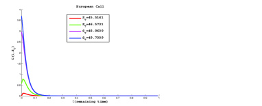
Figure 1: Call price for four diffrents values of spot price at maturity versus remaining time to maturity
Refer to caption
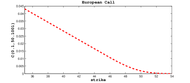
Figure 2: Comparison of call values for four diffrents values of spot price at maturity versus remaining time to maturity

Figure 1 plots call option for different spot price of the underlying at maturity versus remaining time. Note that, as remaining time increase the mean-reverting and price-cap effect in all four case cause the call prices converge to zero under the set parameters gived above. Figure 2 give comparison between illustrative curve of call for four different electricity spot price at maturity. This two figures illustrate that for different initials conditions call option prices converge verse to the same value. From this we can thus, say that different properties shown theoretically are effective under the established conditions.
Refer to caption
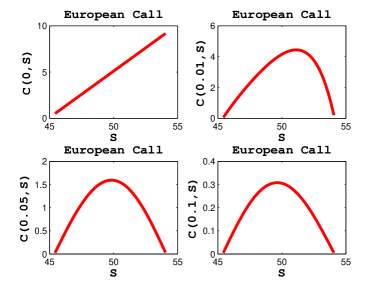
Figure 3: Call price for four different remaining time to maturity versus spot price
Refer to caption
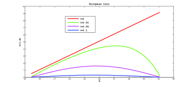
Figure 4: Comparison of call price for four different versus spot price

Figure 3 and 4 illustrate a reality enough close to those in the classical financials markets. In the sens that in financial market the values of call option before the maturity evolved in the form of a curve which towards to the payoff line progressively and as we approach maturity.

Refer to caption
Figure 5: Call price for three diffrents values of strike versus spot price S, the other parameters is unchanged as in table 2
Refer to caption
Figure 6: Call price versus strike price K, the other parameters in unchange as in table 2
Refer to caption
Figure 7: Call price versus strike price K, the other parameters in unchange as in table 2

From figures 5, 6 and 7 one can observed that the values of call decrease when strike price increase. This behaviour of the call values is from a risk management point of view what it is wished.
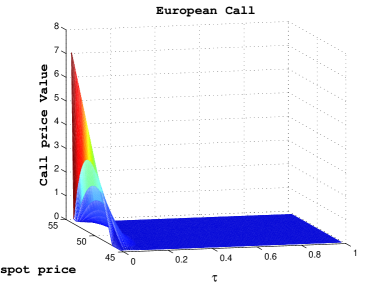
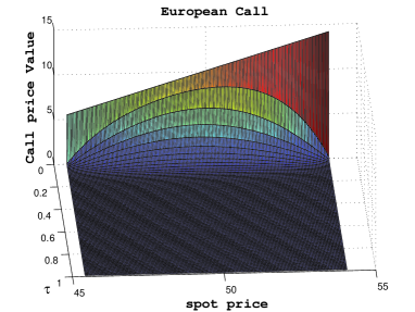
Refer to caption
Figure 8: Call price versus remaining time and spot price σJ=0.5subscript𝜎𝐽0.5\sigma_{J}=0.5, K=45𝐾45K=45, the other parameters is unchanged as in table 2
Refer to caption
Figure 9: Call price versus remaining time and spot price σJ=2.5subscript𝜎𝐽2.5\sigma_{J}=2.5 and K=40𝐾40K=40, the other parameters is unchanged as in table 2

Analysis plots of figures 8 and 9 which illustrate call option price as a function of remaining time and spot price one can said that for a large remaining time jumps effects are not perceptible and then can effect call. Whereas a small remaining time to maturity call prices increase suddenly which express the effect of jump. We must therefore say that the jump term which allows to take into account certain reality of the electricity market is not inconsiderable since that it impact on the call prices are quite noticeable.

6 Discussion and Conclusion

The characterization of european options prices in terms of the classical solution, or, in general, in the terms of the viscosity solution of a PIDE allows the use of numerical methods to obtain efficient approximations of option values. This has been a centre of research in recent times in the case of exponential Lévy models with finite arrival or infinite arrival rate of jumps. Some authors use the finite difference method to approximate the PIDE solution (see [2]), while others like [12] approximate viscosity solutions in the case of nonsmoothness of option prices. In both cases, success (in terms of efficient approximation) has been obtained. In this paper we used their approach to evaluate European call option when the underlying is electricity. The motivation behind our approach arose from the fact that the electricity prices model presented here, by hypothesis, possesses most of the properties (as in their case) of an exponential Lévy model, and the Markov process property. We focus on the pricing of call option because put option can be deduced from the put-call using parity formula. In the mathematical point of view, numerical results have confirmed the established theoretical results. In the finance point of view, numerical results present an interpretation which was coherent with some realities in the electricity market, when it is regulated under price cap.

A limitation of this work is that it can be adapted only to option pricing with short maturity in a regulated market. In future work, we plan to study option pricing on future option.

Acknowledgements

We thank the African Center of Excellence in Technologies, Information and Communication ( CETIC ) which placed at our disposal its infrastructures. This helped us to improve conditions of work.

References

  • [1] J. Acton and I. Vogelsang, Symposuim on Price Cap Regulation: Introduction, Rand Journal of Economics, Vol.20, page 369, 1989.
  • [2] O. Alvarez and A. Tourin, Viscosity solutions of nonlinear integro-differential equation, Annales de l’Institut Henri Poincaré,13(3), pp. 293-317, 1996.
  • [3] H. Amann, Linear and Quasilinear Parabolic Problems: Abstract Linear Theory, Birkhäuser Vol. 1., 1995.
  • [4] F. Black and M. Scholes, The Pricing of options and Corporate Liabilities, The journal of Political Economy, Vol. 81, No. 3, pp. 634-654, 1973.
  • [5] D. Bates, Jumps and stochastic volatility: Exchange rate processes implicit in Deutchemark option, Review of Financial Studies, 9, 69-108, 1996.
  • [6] G. Bales, R. Buckdahn, and E. Pardoux, Backward Stochastic Differential Equations and Integral-Partial Differential Equations, Stochast. Stochast. Reports 60, 57-83, 1997.
  • [7] G. Barles and P. E. Souganidis, Convergence of Approximation Schemes for Fully Nonlinear Second Order Equations, Asymptotic Anal., pp. 271-283, 1991.
  • [8] A. Cartea, M. Figueroa, Pricing in electricity markets: A mean reverting jump diffusion model with seasonality., Applied Mathematical Finance 12(4), 313-335, 2005.
  • [9] P. Carr and D. B. Madan, Option Valuation using the Fast Fourier Transform, Journal of Computational Finance, 2, N0superscript𝑁0N^{0}.4, Summer 61-73, 1999.
  • [10] Chiarella, carl, Ziogas and Andrew, American call options under jump-diffusion processes- A Fourier transform approach, Appl. Math. Finance, Vol. 16, no. 1, pp37-79, 2009.
  • [11] R. Cont, Ekaterina voltchkova, Integro-differential equation for option prices in exponential Lévy models, Finance and Stochastics,Springer, 2005.
  • [12] R. Cont, Ekaterina voltchkova, A Finite difference scheme fo option pricing in jump diffusion and exponential Lévy models, Siam J. Numer. Anal. Vol. 42, No. pp.1596-1626, 2005.
  • [13] M. G. Crandall, H. Ishi, and P. L. Lions, User’s Guide to Viscosity Solutions of Second Oder Partial Differential Equations, New Series of the American Mathematical Society, Vol. 27, Number 1, 1992.
  • [14] S. Deng, Pricing electricity derivatives under alternative stochastic spot price models, Proceedings of the 33rd Hawaii Internatioal Conference on system Sciences, 2000.
  • [15] A. Etheridge, A Course in Financial Calculus, Cambridge University Press,first edition, 2002.
  • [16] ENMAX, Power Corporation 2007-2016 formula Based Ratemaking, Alberto Utilities Commission, Decision N0. 2009-035, 2009.
  • [17] A. Hirsa and D.B. Madan, Pricing American option under Variance Gamma, Journal of Computational Finance, vol. 7, pp. 63-80, 2004.
  • [18] J. Jacod and A. N. Shiryaev, Limit Theorems for Stochastic Processes, Springer, Berlin, 2nd edition, 2002.
  • [19] P.L. Joskow, Incentive Regulation and its Application to Electricity Networks, Review of Network Economics, vol 7,Issue 4, 2008.
  • [20] P.L. Joskow, Incentive Regulation in Theory and Pratice: Electricity Distribution And Transmission Network, Prepared for the National bureau of Economic Reseach on Economic Conference Regulation, Working Paper 05-18, Brooking Joint Center for Regulatory Studies, Washington DC, 2005.
  • [21] J. J. Laffont, J. Tirole, A Theory of Incentives in Procurement and Regulation, MIT Press, Cambridge, MA, 1993.
  • [22] A. Lewis, A Sample option Formula for General Jump-Diffusion and other exponential Lévy processes, www.optioncity.net, Working paper, 2001.
  • [23] S. Littlechild, Regulation of British Telecommunication’Profitability. Tech. Rep., Department of Industry, London, 1983.
  • [24] D. B. Madan, P. Carr and E. C. Chang, The Variance gamma process and option pricing, European Finance Review, 2, 79-105.
  • [25] C. Merton, Continuous-Time Finance, Harvard University, First revised edition, 2001.
  • [26] D. Nualart and W. Schoutens, Backward stochastic differential equations and Feynman-Kac formula for Lévy processes, with applications in finance, Bernoulli 7(5), 761-776, 2001.
  • [27] Polipovic Dragana, Energy Risk: Valuing and Managing Energy Derivatives The Mac-Graw Hill Companies, 2007.
  • [28] C.Rama, P. Tankov, Financial modelling with jump processes, Chapman and Hall/CRC press, 2003.
  • [29] K. Sato, Lévy Processes and Infinitely Divisible Distributions, Cambridge University Press, 1999.
  • [30] L. Scott, Pricing stock in a jump-diffusion model with stochastic volatility and interest rate: Application of Fourier inversion methods, Mathematical Finance, 7, 413-426, 1997.
  • [31] H. Wong and P. Guan, An FFT network for Lévy option pricing, Journal of Banking and Finance, Vol. 35, no. 4, pp. 988-999, 2011.