Constrained transport and adaptive mesh refinement in the
Black Hole Accretion Code

Abstract

Context. Worldwide very-long-baseline radio interferometry (VLBI) arrays are expected to obtain horizon-scale images of supermassive black hole candidates as well as of relativistic jets in several nearby active galactic nuclei. This, together with the expected detection of electromagnetic counterparts of gravitational-wave signals, motivates the development of models for magnetohydrodynamic flows in strong gravitational fields.

Aims. The Black Hole Accretion Code (BHAC) is a publicliy available code intended to aid with the modelling of such sources by performing general relativistic magnetohydrodynamical (GRMHD) simulations in arbitrary stationary spacetimes. New additions to the code are required in order to guarantee an accurate evolution of the magnetic field when small and large scales are captured simultaneously.

Methods. We discuss the adaptive mesh refinement (AMR) techniques employed in BHAC, essential to keep several problems computationally tractable, as well as staggered-mesh-based constrained transport (CT) algorithms to preserve the divergence-free constraint of the magnetic field, including a general class of prolongation operators for face-allocated variables compatible with them.

Results. After presenting several standard tests for the new implementation, we show that the choice of divergence-control method employed can produce qualitative differences in the simulation results for scientifically relevant accretion problems. We demonstrate the ability of AMR to decrease the computational costs of black-hole accretion simulations while sufficiently resolving turbulence arising from the magnetorotational instability. In particular, we describe a simulation of an accreting Kerr black hole in Cartesian coordinates using AMR to follow the propagation of a relativistic jet while self-consistently including the jet engine, a problem set up-for which the new AMR implementation is particularly advantageous.

Conclusions. The CT methods and AMR strategies discussed here are being currently employed in the simulations performed with BHAC used in the generation of theoretical models for the Event Horizon Telescope Collaboration.

1 Introduction

The prospects of horizon-scale images of the two nearest supermassive black hole (SMBH) candidates Sgr A* and M 87, soon to be obtained by very-long-baseline interferometry (VLBI) arrays (Doeleman et al. 2008; Akiyama et al. 2015; Fish et al. 2016; Goddi et al. 2017; Issaoun et al. 2019), open the possibility to study in great detail both fundamental and astrophysical aspects of these objects. Among the most exciting possibilities are direct observations of the black-hole shadow (Abdujabbarov et al. 2015; Younsi et al. 2016; Psaltis et al. 2016, 2015; Mizuno et al. 2018) or the movement of hot spots in the accretion flow (Broderick & Loeb 2006), as well as deciphering the cause of flares and non-thermal emission mechanisms (Özel et al. 2000; Dexter et al. 2012; Davelaar et al. 2018, 2019). In addition to Sgr A* and M 87, VLBI observations will provide high-resolution images of other sources of great interest. For instance, observations of the two-sided jet in the nearby active galactic nucleus (AGN) Cen A (Kim et al. 2018) offer unique possibilities to study the the dynamics of jet formation and propagation in these objects. VLBI images could also be crucial to discriminate between models for the periodic variability in the BL Lac object OJ287, namely a secondary SMBH plowing through the accretion disk (Valtonen et al. 2008), or a precessing disk (Katz 1997) or jet (Britzen et al. 2018).

General-relativistic magnetohydrodynamical (GRMHD) simulations are an invaluable tool and possibly the only available one to assess the validity of theoretical models with respect to astronomical observations; however, an important challenge for codes performing such simulations is the interplay between different scales relevant for the accretion process. Such a large excursion of lengthscales can easily make some problems prohibitive even for massively parallel numerical simulations. In fact, to aid with the interpretation of astronomical observations, simulations of accretion flows must reproduce global quantities of the system, such as accretion rates, spectra and light curves, or large-scale features such as the position of re-collimation shocks in the jet. However, many of these observables are determined by turbulent phenomena occurring at much smaller scales, which must be resolved to a reasonable degree to properly reproduce the physics. For instance, the mechanism of angular momentum transport that permits accretion (Shakura & Sunyaev 1973) is now believed to be magnetic turbulence driven by the the magnetorotational instability (MRI, Balbus & Hawley 1991), and the processes re-collimating the jet and leading to equipartition (Porth & Komissarov 2015), are driven by several magnetohydrodynamical instabilities (see e.g.,  Mizuno et al. 2012) which interact with the acceleration processes (see e.g.,  Aloy & Rezzolla 2006).

By concentrating resolution only at places where it is most needed, Adaptive Mesh Refinement (AMR) offers a flexible solution to this problem. In addition, a great advantage of AMR is the possibility of the grid to follow moving features while applying sufficient resolution. This can be of special importance, for instance, for systems with complex geometries, such as precessing jets (Britzen et al. 2018; Liska et al. 2018) and discs (Fragile et al. 2007; McKinney et al. 2013) or tidal disruption events (Tchekhovskoy et al. 2014).

Among the variety of GRMHD codes reported on the literature (Hawley et al. 1984; Kudoh 2000; De Villiers & Hawley 2003; Gammie et al. 2003; Baiotti et al. 2005; Duez et al. 2005; Anninos et al. 2005; Antón et al. 2006; Mizuno et al. 2006; Del Zanna et al. 2007; Giacomazzo & Rezzolla 2007; Radice & Rezzolla 2012; Radice et al. 2014; McKinney et al. 2014; Etienne et al. 2015; Zanotti & Dumbser 2015; White et al. 2016; Meliani et al. 2017; Anninos et al. 2017; Liska et al. 2018; Fambri et al. 2018) an increasing number is making use of AMR techniques, (see e.g.,  Anninos et al. 2005; Zanotti et al. 2015; White et al. 2016; Liska et al. 2018). One of them is the publicly available BHAC (the Black Hole Accretion Code, www.bhac.science), which was described in Porth et al. (2017) and is the main focus of this work. The consistency of results obtained by several of the codes in this list is thoroughly analyzed in the forthcoming work of Porth et al. (2019).

An important challenge to the application of AMR in GRMHD simulations comes from the solenoidal constraint of the magnetic field, $\nabla\cdot\boldsymbol{B}=0$, which must be fulfilled in order for the simulation to represent a physical state. The numerous schemes devised to enforce this constraint present different degrees of complication to be coupled with AMR techniques. Divergence-cleaning schemes, which require only the solution of an additional equation damping and propagating away violations to the constraint, can be coupled straightforwardly to AMR grids, as done by Anninos et al. (2005); Zanotti et al. (2015); Porth et al. (2017).

Unfortunately, comparisons among several schemes in non-relativistic magnetohydrodynamics (Toth 2000; Balsara & Kim 2004; Mocz et al. 2016) show that all tested variants of the divergence-cleaning method produce important spurious oscillations in the magnetic-field energy. Balsara & Kim (2004) have attributed these oscillations to the non-locality introduced by the constraint-damping equation, thus suggesting that all divergence-cleaning methods may suffer from the same problem. In a previous work (Porth et al. 2017), we have observed the same behaviour in GRMHD when comparing simulations on uniform grids performed using the divergence-cleaning technique known as Generalized Lagrange Multipliers (GLM, Dedner et al. 2002) and the method known as flux-interpolated Constrained Transport (flux-CT, Toth 2000).

By adopting a discretisation of Faraday’s law consistent with that of the constraint, Constrained-Transport (CT) methods maintain the solenoidal condition to machine precision throughout the solution of the GRMHD equations. In general, this requires to define the components of the magnetic field at cell faces, in a grid that is staggered with respect to that of the hydrodynamic variables.

A drawback of these methods is that the fulfilment of the constraint at every next step depends on its fulfilment at the current step; therefore, the initial condition must be divergence-free and care must be taken in order not to generate magnetic-field divergence by any other means. This can happen, in particular, at boundary cells, at coarse/fine interfaces in AMR simulations, and when creating and destroying blocks at prolongation (refining) and restriction (coarsening). Although the generation divergence at resolution jumps can by avoided by advancing in time the magnetic vector potential and computing the magnetic field as its curl (Etienne et al. 2010), the method is sensitive to the gauge condition employed, giving especially bad results for gauges with zero-speed modes (Etienne et al. 2012).

Furthermore, even though cell-centred versions of these methods exist (Toth 2000) and have been applied in GRMHD codes (see e.g.,  Gammie et al. 2003; Mizuno et al. 2006; Porth et al. 2017), these are incompatible with AMR, since the problem of finding divergence-preserving prolongation and restriction operation for cell-centred magnetic fields is under-determined, i.e., information is lost when abandoning the face representation in favour of the cell-centred representation (Tóth & Roe 2002).

The approach used in this work consists in applying divergence-preserving restriction and prolongation operators for face-allocated magnetic fields. Examples of these operators were derived independently by Tóth & Roe (2002) and Balsara (2001), and have been employed in codes such as BATSRUS (Tóth et al. 2012) and AstroBEAR (Cunningham et al. 2009).

In addition, staggered magnetic fields allow the use of upwind magnetic field evolution schemes. In fact, as shown by Flock et al. (2010), not-upwind algorithms such as the widely used flux-CT and the Balsara & Spicer (1999) method (BS) are prone to numerical instabilities. Upwind CT schemes include the second-order algorithm by Gardiner & Stone (2005), used for example in Athena++ (White et al. 2016), and the two algorithms presented in Londrillo & Del Zanna (2004) and in Del Zanna et al. (2007), which allow the use of high-order schemes for the integration of Faraday’s law.

This work largely focuses on the AMR-compatible implementation of staggered grids and the upwind CT methods by Londrillo & Del Zanna (2004) and Del Zanna et al. (2007) in BHAC. Special attention is given to a new derivation of divergence-preserving prolongation operators, which constitute a coordinate-independent generalisation of those found in the literature for the special case of Cartesian geometry (Tóth & Roe 2002).

Though these methods are fully general, technical details on their implementation in BHAC are provided, with the purpose of documenting how they can be incorporated in a GRMHD code. These include the ghost-cell exchange, the data structures and the special treatments employed at coarse/fine interfaces, and at the polar axis. The new methods implemented in the code are validated through several tests, which are also used to highlight the differences between the newly implemented schemes and those already present and validated. In particular, we present simulations of magnetised accretion onto a Kerr black hole, which take advantage of the newly implemented methods. This problem is of central importance for the interpretations of future images to be obtained by the EHT, and constitutes the main scientific application of the code. As shown later, we find that the divergence control technique employed significantly affects the dynamics of this system.

Moreover, the use of AMR makes it possible to simulate this system in Cartesian coordinates while still resolving the growth of the MRI with sufficient accuracy to reproduce the same mass-accretion rate and fluxes through the horizon found in spherical coordinates. This might be useful to avoid and possibly quantify directional biases introduced by grids in spherical coordinates, such as those commonly used in simulations of the accretion process, or eliminate the need of special boundary conditions in the vicinity of the polar axis.

This work is organised as follows: Section 2 presents the formulation of the equations of GRMHD employed in BHAC, as well as a brief description of the coordinates and equations of state available in the code. Section 3 summarizes the numerical methods used to solve these equations, namely finite-volume (Section 3.1) and CT methods (Section 3.2). The mathematical and technical aspects of BHAC’s AMR-compatible implementation of staggered grids is contained in Section 4, with Section 4.2 focusing on the new prolongation operators. Section 5 presents the problems used to validate the new methods, while the simulations of accretion onto black holes using the newly implemented methods are described in Section 6. Finally, in Section 7 we summarise and discuss the prospects of future research.

Hereafter, we use Greek symbols for spacetime indices that run from 0 to 3 and Latin symbols for for hypersurface indices, that run form 1 to 3.

2 Mathematical formulation

2.1 Equations of GRMHD

BHAC was initiated as an extension of the MPI-AMRVAC framework towards GRMHD simulations in 1, 2, and 3 dimensions using finite-volume methods and a variety of modern numerical methods, described more in detail in Porth et al. (2017). It exploits much of MPI-AMRVAC’s infrastructure for parallelisation and block-based automated Adaptive Mesh Refinement (AMR), resulting in a potentially significant saving in computational time and computing resources. BHAC solves the equations of ideal magnetohydrodynamics (MHD) in general relativity but also in more generic spacetimes (Mizuno et al. 2018). The GRMHD equations are expressed as conservation equations for the rest-mass density, the energy and momentum, and the homogeneous Maxwell equations

$$\begin{split}\nabla_{\mu}(\rho u^{\mu})=&\ 0\,,\\ \nabla_{\mu}T^{{\mu\nu}}=&\ 0\,,\\ \nabla_{\mu}\,^{*}\!F^{\mu\nu}=&\ 0\,,\end{split}$$ (1)

where $\rho$ is the particle number density in the fluid frame, $u^{\mu}$ is the fluid 4-velocity in the observer frame, $T^{\mu\nu}$ is the energy-momentum tensor and ${}^{*}\!F^{\mu\nu}$ is the dual of the Faraday tensor.

The Faraday tensor $F^{\mu\nu}$ and its dual ${}^{*}\!F^{\mu\nu}$ are such that the electric and magnetic fields measured by an observer moving at 4-velocity $U^{\mu}$ are

$$E^{\mu}\coloneqq F^{\mu\nu}U_{\nu}\ \ \text{and}\ \ B^{\mu}\coloneqq^{*}\!F^{\mu\nu}U_{\nu}\,.$$ (2)

and are related as ${}^{*}\!F^{\mu\nu}\coloneqq\frac{1}{2}\epsilon^{\mu\nu\alpha\beta}F_{\alpha\beta}$ where $\epsilon^{\mu\nu\alpha\beta}$ are the components of the Levi-Civita tensor. Therefore, in a general frame moving with 4-velocity $U^{\mu}$

$$F^{\mu\nu}\coloneqq U^{\mu}E^{\nu}-U^{\nu}E^{\mu}-\epsilon^{\mu\nu\lambda\delta}U_{\lambda}B_{\delta}\,,$$ (3)

and

$${}^{*}\!F^{\mu\nu}\coloneqq U^{\mu}B^{\nu}-U^{\nu}B^{\mu}+\epsilon^{\mu\nu\lambda\delta}U_{\lambda}E_{\delta}\,.$$ (4)

Instead of solving the inhomogeneous Maxwell equations, we close the system by enforcing the ideal-MHD condition

$$e^{\mu}=F^{\mu\nu}u_{\nu}=0\,,$$ (5)

where $e^{\mu}$ denotes the electric field in the fluid frame. Consequently, the magnetic field in the fluid frame is $b^{\mu}=^{*}\!F^{\mu\nu}u_{\nu}$ and

$${}^{*}\!F^{\mu\nu}=b^{\mu}u^{\nu}-b^{\nu}u^{\mu}\,.$$ (6)

Physically, the ideal-MHD condition corresponds to a plasma with an infinite conductivity and has the important consequence that in this case the magnetic field is simply advected with the fluid (frozen-flux theorem).

The energy-momentum tensor $T^{\mu\nu}$ includes both fluid and electromagnetic contributions. Using equation (6) to write its electromagnetic part in terms of $b^{\mu}$ only (Anile 1990), it reads

$$T^{\mu\nu}=\rho h_{\rm tot}u^{\mu}u^{\nu}+p_{\rm tot}g^{\mu\nu}-b^{\mu}b^{\nu}\,.$$ (7)

where $h_{\rm tot}\coloneqq h+b^{2}/\rho$ is the total specific enthalpy and $p_{\rm tot}=p+b^{2}/2$ is the total pressure, both in the fluid frame.

The system is closed once an equation of state relating the specific enthalpy of the fluid with the density and the pressure $h=h(\rho,p)$ is specified. The equations of state for an ideal gas, a Synge gas and a polytropic fluid are currently implemented in BHAC (see Porth et al. 2017, for more details), although the implementation of any additional one is straightforward as long as it is analytic. Additionally, BHAC can be used together with the microphysics routines developed in Most et al. (2019) that can handle temperature-dependent equations of state and provide a neutrino leakage scheme (Ruffert et al. 1996; O’Connor & Ott 2010; Galeazzi et al. 2013).

In order to formulate system (1) as a set of evolution equations, we employ the 3+1 decomposition of the spacetime (see, e.g.,  Alcubierre 2008; Rezzolla & Zanotti 2013). The metric is decomposed as $g_{\mu\nu}=\gamma_{\mu\nu}-n_{\mu}n_{\nu}$, where $n_{\mu}$ and $\gamma_{\mu\nu}$ are such that $\gamma_{\mu}\,^{\nu}n_{\nu}=0$ and $n_{\nu}n^{\nu}=-1$. Thus, $\gamma_{\mu}\,^{\nu}$ defines a projection operator onto a hypersurface normal to the vector field $n^{\nu}$ and contains the 3-metric induced in the hypersurface.

The explicit form of the line element in a 3+1 split spacetime is

$$ds^{2}=-\alpha^{2}dt^{2}+\gamma_{ij}(dx^{i}+\beta^{i}dt)(dx^{j}+\beta^{j}dt)\,,$$ (8)

where $\alpha$ and $\beta^{i}$ are the lapse and the shift vector, respectively. Using $\gamma_{\mu}\,^{\nu}$ and $n_{\nu}$, it is possible to define variables suitable to be evolved. These are the conserved variables in the Eulerian frame: the number density $D\coloneqq-\rho u^{\nu}n_{\nu}$, the covariant 3-momentum $S_{i}\coloneqq n_{\mu}\gamma_{\nu i}T^{\mu\nu}$, the total energy $U\coloneqq n_{\mu}n_{\nu}T^{\mu\nu}$ and the spatial stress tensor $W^{ij}\coloneqq\gamma_{\mu i}\gamma_{\nu j}T^{\mu\nu}$.

In terms of these variables, system (1) can be written as a set of conservation equations

$$\partial_{t}(\sqrt{\gamma}\boldsymbol{U})+\partial_{i}(\sqrt{\gamma}\boldsymbol{F}^{i})=\sqrt{\gamma}\boldsymbol{S}\,,$$ (9)

in addition to the solenoidal constraint for the magnetic field $\partial_{i}\sqrt{\gamma}B^{i}=0$. Here, $\gamma$ is the determinant of the induced three-metric, and the vectors of conserved quantities $\boldsymbol{U}$, the fluxes $\boldsymbol{F}^{i}$, and the sources $\boldsymbol{S}$ are given by

$$\begin{split}\boldsymbol{U}=\left[\begin{array}[]{c}D\\ S_{j}\\ \tau\\ B^{j}\end{array}\right]\,,\ \qquad\boldsymbol{F}^{i}=\left[\begin{array}[]{c}\mathcal{V}^{i}D\\ \alpha W^{i}_{j}-\beta^{i}S_{j}\\ \alpha(S^{i}-v^{i}D)-\beta^{i}\tau\\ \mathcal{V}^{i}B^{j}-B^{i}\mathcal{V}^{j}\end{array}\right]\,,\\ \boldsymbol{S}=\left[\begin{array}[]{c}0\\ \frac{1}{2}\alpha W^{ik}\partial_{j}\gamma_{ik}+S_{i}\partial_{j}\beta^{i}-U\partial_{j}\alpha\\ \frac{1}{2}W^{ik}\beta^{j}\partial_{j}\gamma_{ik}+W_{i}^{j}\partial_{j}\beta^{i}-S^{j}\partial_{j}\alpha\\ 0\end{array}\right]\,,\end{split}$$ (10)

where $v^{i}\coloneqq\gamma^{i}_{\mu}u^{\mu}/\Gamma$ is the 3-velocity, $\Gamma\coloneqq-u^{\mu}n_{\mu}$ is the Lorentz factor, and $\mathcal{V}^{i}\coloneqq\alpha v^{i}-\beta^{i}$ is the transport velocity. Evolving $\tau\coloneqq U-D$ instead of $U$ makes the evolution more accurate in regions of low energy and allows to recover the Newtonian limit.

To calculate the fluxes $\boldsymbol{F}^{i}$, knowledge of the primitive variables $\boldsymbol{P}=\left[\rho,\Gamma v^{i},p,B^{i}\right]$ is required. While it is straightforward to find $\boldsymbol{U}(\boldsymbol{P})$, $\boldsymbol{P}(\boldsymbol{U})$ requires numerical inversion. The inversion process then consists of finding the auxiliary variables $\boldsymbol{A}=\left[\Gamma,\xi\right]$, where $\xi\coloneqq\Gamma^{2}\rho h$ and $h$ is the specific enthalpy compatible with $\boldsymbol{U}$ and $\boldsymbol{P}$, which is in turn used to find the primitives. Once $\boldsymbol{A}$ is found, BHAC stores it in order to facilitate new inversions, thus extending the array $\boldsymbol{U}(\boldsymbol{P})$, as detailed in Porth et al. (2017).

2.2 Coordinates in BHAC

Table 1: Coordinates available in BHAC: The first column shows the identifier of the coordinates within the code, the second their name, the third whether the metric derivatives are calculated numerically, and the fourth whether they are initialised from the 4-metric $g_{\mu\nu}$.

Identifier	Coordinates	Num. derivatives	Init. $g_{\mu\nu}$
bl	Boyer-Lindquist	No	No
cart	Cartesian	No	No
cks	Cartesian Kerr-Schild (CKS)	Yes	Yes
cmks	Cylindrified modified Kerr-Schild	Yes	No
dleh	Non-rotating dilaton black hole (García et al. 1995)	No	No
ht	Hartle-Thorne (Hartle & Thorne 1968)	Yes	Yes
ks	Kerr-Schild	No	No
lrzks	Horizon penetrating Rezzolla & Zhidenko coordinates	Yes	Yes
mks	Modified Kerr-Schild (MKS, McKinney & Gammie 2004)	No	No
num	Numerical	Yes	Yes/No
rns	RNS (Stergioulas & Friedman 1995)	Yes	No
rz	Rezzolla & Zhidenko parametrization (Rezzolla & Zhidenko 2014)	Yes	No
sp	Spherical coordinates	No	No
ss	Schwarzschild coordinates	No	No

The main target application of BHAC is the simulation of accretion onto compact objects in arbitrary spacetimes. This has allowed to simulate accretion onto Kerr black holes to build theoretical models of M 87 (Davelaar et al. 2019), but also to explore the consequences of alternative theories of gravity (Mizuno et al. 2018) or of the presence of a boson star (Olivares et al. 2018) at the Galactic Center in the forthcoming horizon-scale VLBI images of Sgr A*, as well as the study of quasi-periodic oscillations in accretion discs around neutron stars (de Avellar et al. 2018).

As a result, BHAC is designed with a great flexibility to adopt new spacetime metrics. Its modular structure not only allows us to add straightforwardly new analytic coordinates, but another interesting feature is that it is not compulsory to provide derivatives of the metric, which are used to calculate the sources. The user needs only to provide the metric functions, and derivatives can be calculated internally using the complex-step derivative (Squire & Trapp 1998), a highly accurate numerical method which is capable of achieving machine precision for derivatives of algebraic functions (Martins et al. 2003).

The code can handle spacetime metrics given either in 3+1 form (i.e., expressed in terms of $\gamma_{ij}$, $\beta_{i}$ and $\alpha$) or as the full 4-metric $g_{\mu\nu}$, as the necessary conversions to 3+1 form are done internally. In addition, it is able to read tabulated numerical metrics when the spacetime is known only numerically. A list of metrics currently available in the code is reported in Table 1, which complements that presented in Porth et al. (2017).

The need to store the metric components both at barycentre positions and at cell interfaces is handled efficiently by adopting the metric data structure described in Porth et al. (2017), which takes advantage of the symmetry of the metric components and the fact that the metric and its derivatives are usually sparsely populated, i.e., many of the tensor components are zero.

2.2.1 Modified Kerr-Schild coordinates

Due to its use in later parts of this work, we next describe the less well known modified Kerr-Schild coordinates (MKS). MKS coordinates $x^{\mu}=(t_{\rm MKS},s,\vartheta,\phi_{\rm MKS})$ were introduced by McKinney & Gammie (2004) in order to simulate large domains and, at the same time, concentrate the resolution near the black hole and on the equatorial plane. They are related to the standard Kerr-Schild coordinates $x^{\mu^{\prime}}=(t_{\rm KS},r_{\rm KS},\theta_{\rm KS},\phi_{\rm KS})$ by the transformation

$$\begin{split}t_{\rm KS}&=\ t_{\rm MKS}\,,\\ r_{\rm KS}&=\ R_{0}+e^{s}\,,\\ \ \theta_{\rm KS}&=\ \vartheta+\frac{{\vartheta_{0}}}{2}\sin(2\vartheta)\,,\\ \phi_{\rm KS}&=\ \phi_{\rm MKS}\,,\end{split}$$ (11)

where $R_{0}$ and ${\vartheta_{0}}$ are constant parameters. Note that the convention for the parameter ${\vartheta_{0}}$ is different from that used in McKinney & Gammie (2004). The one employed here is chosen so that $\vartheta$ reduces to $\theta_{\rm KS}$ when ${\vartheta_{0}}=0$, thus retrieving logarithmic Kerr-Schild coordinates.

It is worth to mention that, in contrast to Porth et al. (2017), in this work the inverse relation $\vartheta(\theta_{\rm KS})$ is not approximated using a cubic polynomial, but the resulting transcendental equation is solved numerically whenever necessary.

3 Numerical methods

3.1 Finite-volume scheme

To introduce the notation used in this work, we next summarise the finite-volume scheme used by BHAC to evolve the hydrodynamic variables in system (9). This scheme was already described in Porth et al. (2017), to which we refer the reader for more details.

To obtain the discretized equations, the simulation domain is divided into control volumes and the system is integrated over each of them. This leads to evolution equations for the average $\boldsymbol{\bar{U}}_{i,j,k}$ of the conserved quantities inside each cell

$$\begin{split}\frac{d\boldsymbol{\bar{U}}_{i,j,k}}{dt}=-\frac{1}{\Delta V_{i,j,k}}\Biggl{[}&\boldsymbol{F^{1}}\Delta S^{1}\bigr{|}_{i+1/2,j,k}-\boldsymbol{F^{1}}\Delta S^{1}\bigr{|}_{i-1/2,j,k}+\\ &\boldsymbol{F^{2}}\Delta S^{2}\bigr{|}_{i,j+1/2,k}-\boldsymbol{F^{2}}\Delta S^{2}\bigr{|}_{i,j-1/2,k}+\\ &\boldsymbol{F^{3}}\Delta S^{3}\bigr{|}_{i,j,k+1/2}-\boldsymbol{F^{3}}\Delta S^{3}\bigr{|}_{i,j,k-1/2}\Biggr{]}+\boldsymbol{\bar{S}}_{i,j,k}\,.\end{split}$$ (12)

Quantities indicated as, say, $\boldsymbol{F^{1}}\Delta S^{1}\bigr{|}_{i+1/2,j,k}$ represent integrals of the fluxes over the surfaces $\Delta S^{1}\bigr{|}_{i+1/2,j,k}$ bounding the control volume, and $\boldsymbol{\bar{S}}_{i,j,k}$ is the volume average of the sources. Both kinds of integrals are approximated to second order, by assigning to $\boldsymbol{F^{n}}$ ($\boldsymbol{n}=1,2,3$) the point value of the flux at the face center and to $\boldsymbol{\bar{S}}_{i,j,k}$ the point value at the cell barycentre, i.e., at

$$\begin{split}x^{i}_{({\rm face}\ k)}&=x^{i}+\delta^{i}_{k}\frac{\Delta x^{i}}{2}\,,\\ x^{i}_{({\rm barycentre})}&=\frac{\int_{\rm cell}\sqrt{\gamma}\ x^{i}\ dx^{1}dx^{2}dx^{3}}{\int_{\rm cell}\sqrt{\gamma}\ dx^{1}dx^{2}dx^{3}}\,,\end{split}$$

respectively, where $\Delta x^{i}$ is the grid spacing in each direction and $\delta^{i}_{k}$ is Kronecker’s delta. $\boldsymbol{F^{n}}$ is obtained through the approximate solution of a Riemann problem at the interface, and static integrals such as cell volumes, interface areas and barycentre positions are calculated at initialisation using fourth-order Simpson’s rule and stored in memory.

The Riemann solvers currently available in BHAC are the Rusanov method, also known as total variation diminishing Lax-Friedrichs scheme, and the HLL solver of Harten et al. (1983). The left and right states for the Riemann problem are obtained using limited reconstructions from the cell centres (see also Toro 2009; Rezzolla & Zanotti 2013).

BHAC features a variety of reconstruction schemes, some of which are listed in Keppens et al. (2012); Porth et al. (2017). They include both second-order, total variation diminishing (e.g., ‘minmod’, ‘vanLeer’), and high-order such as ‘PPM’ (Colella & Woodward 1984), ‘LIMO3’ (Čada & Torrilhon 2009) and ‘MP5’ (Suresh & Huynh 1997). Recent additions to that list are the high-order schemes WENO5 and WENOZ+ (Acker et al. 2016). Equation 12 can be integrated using any of the methods present in the MPI-AMRVAC toolkit. These include the simple half-step modified Euler, the third order Runge-Kutta RK3 (Gottlieb & Shu 1998) and the strong-stability preserving $s$-step, $p$th-order RK schemes SSPRK($s$,$p$) schemes: SSPRK(4,3), SSPRK(5,4) due to Spiteri & Ruuth (2002) (see Porth et al. 2014, for implementation details).

3.2 Constrained Transport

Constrained transport (CT) is a divergence-control method first proposed by Evans & Hawley (1988). In essence, instead of eliminating the divergence of the magnetic field once it is created, it modifies the way in which magnetic-field transport is evolved so as to prevent the creation of divergence. CT is able to keep a discretisation of $\nabla\cdot\boldsymbol{B}=0$ to a precision close to that of floating point operations by ensuring that the sum of the magnetic fluxes through the surfaces bounding a cell is zero to machine precision. Recalling the definition of the divergence of a vector field $\boldsymbol{B}$

$$\nabla\cdot\boldsymbol{B}=\lim\limits_{\Delta V\rightarrow 0}\frac{1}{\Delta V}\oint_{S=\partial\Delta V}\mkern-27.0mu\boldsymbol{B}\cdot\boldsymbol{n}\,dS\,,$$ (13)

is equivalent to $\nabla\cdot\boldsymbol{B}=0$ in the continuous limit. When the limit is not taken, i.e., for the finite-volume case, it follows from the divergence theorem that the average value of the divergence $\left(\overline{\nabla\cdot\boldsymbol{B}}\right)_{\rm cell}$ is zero within the cell.

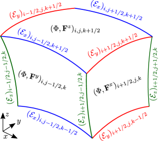
Figure 1: Spatial location of variables for a cell with indices $(i,j,k)$, correspondent to directions $(x,y,z)$, respectively. Line integrals of the electric field $\mathcal{E}$ are located at its edges, and magnetic and numerical fluxes $\Phi$ and $\boldsymbol{F}^{i}$ (the latter used for the BS algorithm) are located at its faces. The conserved hydrodynamic variables belonging to the array $\boldsymbol{U}$, are located at cell centres (not shown).

The central idea from constrained transport is to give the electromagnetic variables a special spatial location, as depicted in Fig. 1. In particular, to each face of the cell corresponds a magnetic flux calculated, for example, as

$$\Phi_{i+1/2,j,k}=\int_{\partial V(x^{1}_{i+1/2})}\gamma^{1/2}B^{1}dx^{2}dx^{3}\,,$$ (14)

and on each edge is associated a line integral of the electric field, similar to

$$\mathcal{E}_{i+1/2,j+1/2,k}=-\int_{x^{3}_{k-1/2}}^{x^{3}_{k+1/2}}\left.E_{3}\right|_{x^{1}_{i+1/2},x^{2}_{j+1/2}}dx^{3}\,.$$ (15)

The magnetic flux at each face is updated from the circulation of the electric field, using the integral form of Faraday’s law

$$\frac{d}{dt}\Phi_{i+1/2,j,k}=\phantom{-} \mathcal{E}_{i+1/2,j+1/2,k}-\mathcal{E}_{i+1/2,j-1/2,k}$$ (16)

$$-\, \mathcal{E}_{i+1/2,j,k+1/2}+\mathcal{E}_{i+1/2,j,k-1/2}\,,$$

Since each of the line integrals of the electric field is shared by two faces, but appears with opposite sign in the time update formula for each of them, the rate of change of $\left(\overline{\nabla\cdot\boldsymbol{B}}\right)_{\rm cell}$, which can be calculated as the sum of the rate of change of the outgoing flux through all faces, vanishes. Therefore, the CT time update ensures that $\left(\overline{\nabla\cdot\boldsymbol{B}}\right)_{\rm cell}$ is kept constant at machine precision from one iteration to the next.

In order for $\boldsymbol{B}$ to be divergence-free during the whole simulation, $\left(\overline{\nabla\cdot\boldsymbol{B}}\right)_{\rm cell}$ must be zero at the initial condition. This can be accomplished by initialising the line integrals of magnetic vector potential along cell edges and calculating the initial magnetic fluxes as the circulation of the vector potential around the cell faces, in the same way as the rate of change of the magnetic flux is calculated from the circulation of the electric field.

After the time update, the magnetic field is interpolated to the cell center in order to use it for the inversion from conserved to primitive variables.

The idea of staggering the magnetic components of the electromagnetic field to achieve a divergence-free evolution to machine precision was first proposed by Yee (1966). However, although his method was widely known in engineering, a staggered grid was not applied in GRMHD until the work of Evans & Hawley (1988).

In the formulas written so far, no approximations have been made. Approximations come into play when deciding how to calculate the line integrals of the electric field. The way these approximations are done distinguishes the different ‘variants’ of CT. Three of these variants are described in the following sections.

3.3 Arithmetic averaging (BS)

This variant was introduced by Balsara & Spicer (1999). In the comparison work of Toth (2000), it is referred to as Flux-interpolated Constrained Transport (flux-CT), although in most of the literature this name is used exclusively for the cell-centered version of this method, proposed also in Toth (2000). In this work, we will use the abbreviation ‘flux-CT’ to refer to the cell-centered version of the method and ‘BS’ to refer to the staggered one. Both variants are particularly suitable for finite-volume schemes, since the electric field at cell edges is estimated as the arithmetic average of the numerical fluxes returned by the Riemann solver. In fact, the numerical fluxes corresponding to the magnetic-field components are surface integrals of the electric field, for example, the flux in the $x^{2}$-direction for $B^{1}$ is

$$\left.\Delta S^{2}\bar{F}^{2}\right|_{i,j+1/2,k}=\int_{x^{1}_{i-1/2}}^{x^{1}_{i+1/2}}\int_{x^{3}_{k-1/2}}^{x^{3}_{k+1/2}}\left.E_{x^{3}}\right|_{j+1/2}\,dx^{3}\,dx^{1}\,.$$ (17)

The innermost integral is the same as that of Eq. (15), so the average flux can be interpreted as

$$\left.\Delta S^{2}\bar{F}^{2}\right|_{i,j+1/2,k}=-\Delta x_{i}\,\tilde{\mathcal{E}}_{i,j+1/2,k}\,,$$ (18)

where $\tilde{\mathcal{E}}_{i,j+1/2,k}$ is the mean value of the integral from Eq. (15) over the face at $j+1/2$. To second-order accuracy, this integral takes the value $\tilde{\mathcal{E}}_{i,j+1/2,k}$ at the middle of the cell. Therefore, $\mathcal{E}_{i+1/2,j+1/2,k}$ can be found by interpolating the averaged fluxes from the four adjacent cell faces as

$$\begin{split}\mathcal{E}_{i+1/2,j+1/2,k}=\frac{1}{4}\Biggl{(}&\frac{\Delta S^{2}\bar{F}^{2}\bigr{|}_{i,j+1/2,k}}{\Delta x_{i}}+\frac{\Delta S^{2}\bar{F}^{2}\bigr{|}_{i+1,j+1/2,k}}{\Delta x_{i+1}}\\ -&\frac{\Delta S^{1}\bar{F}^{1}\bigr{|}_{i+1/2,j,k}}{\Delta y_{j}}-\frac{\Delta S^{1}\bar{F}^{1}\bigr{|}_{i+1/2,j+1,k}}{\Delta y_{j+1}}\Biggr{)}\,.\end{split}$$ (19)

Although this algorithm, especially in its cell-centered version, is widely used in the community (see e.g.,  Gammie et al. 2003; Noble et al. 2009), it is known to lack a proper upwinding and to not reduce to the correct limit for one-dimensional flow (Gardiner & Stone 2005), as well as to cause numerical instabilities (Flock et al. 2010). Efforts to overcome this problems motivated the development of methods such as those by Gardiner & Stone (2005); Londrillo & Del Zanna (2004); Del Zanna et al. (2007). In the next section, we will briefly describe the methods by Londrillo & Del Zanna (2004) and Del Zanna et al. (2007), which we have also implemented in BHAC.

3.4 Upwind constrained transport (UCT)

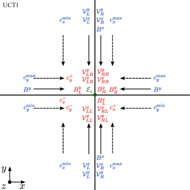
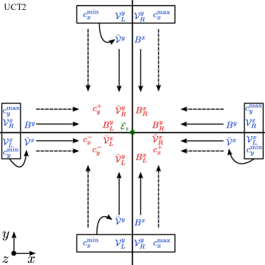
Figure 2: Reconstruction of quantities for UCT1 (left) and UCT2 (right). Quantities in blue are defined at cell faces in $x$ and $y$ and quantities in red at the cell edge in $z$. The resulting line integral of the electric field $\mathcal{E}_{z}$ over the edge is shown in green. Continuous arrows represent limited reconstructions (steps 2 and 3 of UCT1, and 3 of UCT2) and dashed lines the choice of the maximum value (step 5 of UCT1 and 4 of UCT2, the labels $L$ and $R$ for the characteristic speeds are omitted in the figure to avoid saturation). The average transverse transport velocities needed in UCT2 (step 2) $\bar{\mathcal{V}}^{x,y}$ are computed using the quantities in the boxes.

Upwind Constrained Transport (UCT) is a method to evolve the magnetic field, first proposed in (Londrillo & Del Zanna 2004). As a CT method, like BS, it maintains the divergence of the magnetic field to machine precision; however, it furthermore aims to accurately reproduce the magnetic-field continuity and transport properties by using limited reconstructions. Also, in contrast to arithmetic averaging, UCT reduces to the correct 1-dimensional limit when symmetry in the other two directions is assumed. Two variants of UCT are implemented in BHAC. These are presented in (Londrillo & Del Zanna 2004) and in (Del Zanna et al. 2007), and will be referred, respectively, as UCT1 and UCT2. Now we describe the procedure to obtain $\mathcal{E}$ in each of these algorithms. To simplify the notation, we rename $(x^{1},x^{2},x^{3})$ as $(x,y,z)$. We focus on the calculation of $\mathcal{E}_{z}$, but the other cases can be obtained by iteratively replacing $x\rightarrow y$, $y\rightarrow z$ and $z\rightarrow x$ (see Figure 2). In BHAC, the implementation of UCT1 is as follows:

1. At the time of calculating the numerical fluxes at $x$-interfaces, store the characteristic speeds $c^{\mathrm{min}}_{i}$ and $c^{\mathrm{max}}_{i}$ ($i=x,y,z$) obtained from the Riemann solver, as well as the transport velocity $\mathcal{V}^{x}_{L}$, $\mathcal{V}^{y}_{L}$, $\mathcal{V}^{x}_{R}$, and $\mathcal{V}^{y}_{R}$.

2. Reconstruct transport velocities along direction $y$ towards the edges $z$ and obtain one correspondent to the four states around them $\mathcal{V}^{i}_{LL}$, $\mathcal{V}^{i}_{LR}$, $\mathcal{V}^{i}_{RL}$ and $\mathcal{V}^{i}_{RR}$ ($i=x,y$).

3. Reconstruct the magnetic fields on the faces to the same edges and obtain $B^{x}_{L}$, $B^{x}_{R}$, $B^{y}_{L}$ and $B^{y}_{R}$.

4. Calculate approximations to the electric field on the edge from each of the possible states as

   $$E_{z}^{LL} =\mathcal{V}^{y}_{LL}B^{x}_{L}-\mathcal{V}^{x}_{LL}B^{y}_{L}\,,$$

   $$E_{z}^{LR} =\mathcal{V}^{y}_{LR}B^{x}_{R}-\mathcal{V}^{x}_{LR}B^{y}_{L}\,,$$

   $$E_{z}^{RL} =\mathcal{V}^{y}_{RL}B^{x}_{L}-\mathcal{V}^{x}_{RL}B^{y}_{R}\,,$$

   $$E_{z}^{RR} =\mathcal{V}^{y}_{RR}B^{x}_{R}-\mathcal{V}^{x}_{RR}B^{y}_{R}\,.$$

5. Take the maximum characteristic speeds in each direction from the four states,

   $$c^{-}_{x} =\max{(c^{\mathrm{min}}_{x,\ L},c^{\mathrm{min}}_{x,\ R})}\,,$$

   $$c^{+}_{x} =\max{(c^{\mathrm{max}}_{x,\ L},c^{\mathrm{max}}_{x,\ R})}\,,$$

   $$c^{-}_{y} =\max{(c^{\mathrm{min}}_{y,\ L},c^{\mathrm{min}}_{y,\ R})}\,,$$

   $$c^{+}_{y} =\max{(c^{\mathrm{max}}_{y,\ L},c^{\mathrm{max}}_{y,\ R})}\,,$$

   where $c^{\mathrm{min}}_{i,\ L(R)}$ ($c^{\mathrm{max}}_{i,\ L(R)}$) are defined as positive in the $-i$ ($+i$) direction, and they are zero otherwise.

6. Finally, approximate the electric field, as an average of those at the four states weighted by the characteristic speeds and corrected by the transport of magnetic field, using the formula by Londrillo & Del Zanna (2004):

   $$\begin{split}E_{z}=\sqrt{\gamma}\left[\frac{c^{+}_{x}c^{+}_{y}E_{z}^{LL}+c^{+}_{x}c^{-}_{y}E_{z}^{LR}+c^{-}_{x}c^{+}_{y}E_{z}^{RL}+c^{-}_{x}c^{-}_{y}E_{z}^{RR}}{(c^{+}_{x}+c^{-}_{x})(c^{+}_{y}+c^{-}_{y})}\right.\\ \left.+\frac{c^{+}_{x}c^{-}_{x}}{c^{+}_{x}+c^{-}_{x}}(B^{R}_{y}-B^{L}_{y})-\frac{c^{+}_{y}c^{-}_{y}}{c^{+}_{y}+c^{-}_{y}}(B^{R}_{x}-B^{L}_{x})\right]\,.\end{split}$$ (20)

   Since this is a point value, we take the second order approximation that $\mathcal{E}_{z}=E_{z}\Delta z$ and use it to calculate the circulation.

The implementation of UCT2 is as follows:

1. At the time of calculating the numerical fluxes at each interface, store the characteristic speeds $c^{\mathrm{min}}_{i}$ and $c^{\mathrm{max}}_{i}$ ($i=x,y,z$) obtained from the Riemann solver, and the transverse transport velocities at the left and right states, for example $\mathcal{V}^{y}_{L}$, $\mathcal{V}^{z}_{L}$, $\mathcal{V}^{y}_{R}$, and $\mathcal{V}^{z}_{R}$ for the $x$-interface.

2. Obtain a new transverse transport velocity weighting those of the left and right states by the characteristic speeds (Del Zanna et al. 2007). For the $x$-interface, this is

   $$\bar{\mathcal{V}}^{y,z}=\frac{c^{\mathrm{max}}_{x}\mathcal{V}_{L}^{y,z}+c^{\mathrm{min}}_{x}\mathcal{V}_{R}^{y,z}}{c^{\mathrm{max}}_{x}+c^{\mathrm{min}}_{x}}\,.$$ (21)

3. Reconstruct the magnetic fields and the transport velocities to the edge where $\mathcal{E}_{z}$ needs to be calculated. This gives $B^{x,y}_{L,R}$ and $\bar{\mathcal{V}}^{x,y}_{R,L}$.

4. Take the maximum characteristic speeds in the same way as in step (5) of UCT1.

5. Approximate the electric field using the formula by (Del Zanna et al. 2007):

   $$\begin{split}E_{z}=\sqrt{\gamma}\left[-\frac{c^{+}_{x}\bar{\mathcal{V}}^{x}_{L}B^{y}_{L}+c^{-}_{x}\bar{\mathcal{V}}^{x}_{R}B^{y}_{R}-c^{-}_{x}c^{+}_{x}(B^{y}_{R}-B^{y}_{L})}{c^{+}_{x}+c^{-}_{x}}\right.\\ \left.+\frac{c^{+}_{y}\bar{\mathcal{V}}^{y}_{L}B^{x}_{L}+c^{-}_{x}\bar{\mathcal{V}}^{y}_{R}B^{x}_{R}-c^{-}_{y}c^{+}_{y}(B^{x}_{R}-B^{x}_{L})}{c^{+}_{y}+c^{-}_{y}}\right]\,.\end{split}$$ (22)

   Again, we approximate $\mathcal{E}_{z}=E_{z}\Delta z$ and use it to calculate the circulation.

Since UCT2 appears to be more symmetric than UCT1, we prefer it for the simulations presented in this work. However, it is worth to mention that we did not observe important differences, especially no directional bias, when using with UCT1.

An important difference in our implementation with respect to that of Londrillo & Del Zanna (2004) and Del Zanna et al. (2007) is that in those works the quantities $\sqrt{\gamma}B^{i}$ and not the magnetic fields $B^{i}$ are reconstructed at the edges. We instead, factor the square root of the metric determinant and multiply the whole expression for $E_{z}$ by it at the end. This makes the scheme more consistent when evolving a radial magnetic field in the polar regions, and simplifies the AMR operations at the poles, as will be seen in section 4.5.

4 CT-adapted AMR

Constrained transport schemes ensure that, during evolution, no divergence of the magnetic field is created from one iteration to the next, at machine precision. However, by construction, no mechanism to eliminate divergence that has already been created is present. Therefore, in order to exploit the advantages of constrained transport in an AMR code, it is necessary to resort to prolongation and restriction operators that also preserve the constraint $\nabla\cdot\boldsymbol{B}=0$ to machine precision. In addition, care must be taken to synchronise different representations of the same electric and magnetic field components across fine-coarse interfaces, which is done in a step similar to the refluxing of finite-volume methods. After defining the notation in section 4.1, we here describe in detail such operations.

4.1 Notation

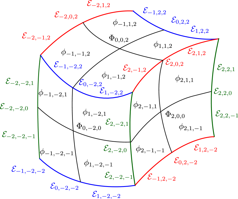
Figure 3: Notation for magnetic fluxes and line integrals of the electric field for section 4.1.

To avoid using lengthy subscripts, we employ a notation similar to that used by Tóth & Roe (2002). We refer to Figure 3 for a schematic view.

The coarse coordinate increment in the direction $i$ is denoted $\Delta X^{i}$ and the correspondent fine increment $\Delta x^{i}=\Delta X^{i}/2$. The center of the coarse cell is defined at $(x_{0}^{1},x_{0}^{2},x_{0}^{3})$ and those of the eight fine cells that result after refinement at $(x_{0}^{1}\pm\Delta x^{1}/2,x_{0}^{2}\pm\Delta x^{2}/2,x_{0}^{3}\pm\Delta x^{3}/2)$. Quantities defined at the fine cell centres are labelled by the subscripts $\pm 1,\pm 1,\pm 1,$ and those at the coarse cell center by $0,0,0$, although this label is often omitted to keep the notation simple. Accordingly, $\Delta V$ is the volume of the coarse cell.

The coarse faces defined by the coordinate surfaces of $x^{1}$ are centered at $(x_{0}^{1}+\Delta X^{1}/2,x_{0}^{2},x_{0}^{3})$. Quantities defined at these faces are labelled by the subscripts $\pm 2,0,0$. For instance, both these faces and their areas are denoted $\Delta S_{\pm 2,0,0}$. The four fine faces in which $\Delta S_{2,0,0}$ is subdivided are labelled $\Delta s_{2,\pm 1,\pm 1}$. The same applies to $\Delta S_{-2,0,0}$ and in the other directions. The twelve fine faces $\Delta s_{0,\pm 1,\pm 1}$, $\Delta s_{\pm 1,0,\pm 1}$ and $\Delta s_{\pm 1,\pm 1,0}$ are not part of any coarse face. The magnetic flux across $\Delta s_{2,1,1}$ is

$$\phi_{2,1,1}=\int_{\Delta s_{2,1,1}}B^{1}\sqrt{\gamma}dx^{2}dx^{3}\,,$$ (23)

and that across $\Delta S_{2,0,0}$ is

$$\Phi_{2,0,0}=\int_{\Delta S_{2,0,0}}B^{1}\sqrt{\gamma}dx^{2}dx^{3}\,.$$ (24)

The same applies to quantities defined at cell edges: $\mathcal{E}_{2,2,0}$ denotes line integral of the electric field along the coarse edge centered at $(x^{1}_{0}+\Delta X^{1}/2,x^{2}_{0}+\Delta X^{2}/2,x^{3}_{0})$ and $\mathcal{E}_{2,2,1}$ that along the fine edge centered at $(x^{1}_{0}+\Delta X^{1}/2,x^{2}_{0}+\Delta X^{2}/2,x^{3}_{0}+\Delta x^{3}/2)$.

In a 2D problem, where symmetry in the $x^{3}$ direction is assumed, the integrals with respect to $x^{3}$ can be ignored, since they only result in multiplying all quantities by a constant factor that is cancelled in every equation.

The divergence of the magnetic field in the coarse cell is discretized as

$$(\nabla\cdot\boldsymbol{B})=\frac{1}{\Delta V}\left(\Phi_{2,0,0}-\Phi_{-2,0,0}+\Phi_{0,2,0}-\Phi_{0,-2,0}+\Phi_{0,0,2}-\Phi_{0,0,-2}\right)\,,$$ (25)

which reduces to the standard definition of divergence (equation 13) in the limit $\Delta V\rightarrow 0$, and corresponding definitions are valid for each of the fine cells.

4.2 Prolongation and restriction operators for face-allocated variables

4.2.1 Restriction formulas

As in Tóth & Roe (2002), to obtain a restriction formula that naturally preserves the divergence, we simply require that the flux through one of the coarse faces is the sum of the fluxes through the fine faces which form part of it, i.e.,

$$\begin{split}\Phi_{\pm 2\,0\,0}=&\sum_{j,k=-1,1}\phi_{\pm 2\,j\,k}\,,\\ \Phi_{0\,\pm 2\,0}=&\sum_{i,k=-1,1}\phi_{i\,\pm 2\,k}\,,\\ \Phi_{0\,0\,\pm 2}=&\sum_{i,j=-1,1}\phi_{i\,j\,\pm 2}\,.\end{split}$$ (26)

The divergence in the newly created coarse cell will be

$$(\nabla\cdot\boldsymbol{B})=\frac{1}{\Delta V}\sum_{i,j,k=-1,1}\Delta V_{i,j,k}(\nabla\cdot\boldsymbol{B})_{i,j,k}\,,$$ (27)

which is consistent with definition (25) since the interior fluxes cancel in pairs. If all $(\nabla\cdot\boldsymbol{B})_{i,j,k}$ are numerical zeros, equation (27) implies that $(\nabla\cdot\boldsymbol{B})$ is as well.

4.2.2 Prolongation formulas

While divergence-free restriction operators can be derived straightforwardly as seen above, it is not trivial to find prolongation operators with the same property. To the best of our knowledge, the only such prolongation operators for vector fields collocated at cell faces are those found by Balsara (2001) and Tóth & Roe (2002), who also derived similar operators for continuous interpolation and for prolongation of vertex-collocated fields. Since the divergence constraint alone results in an under-determined system of equations for the fine magnetic fields, Tóth & Roe (2002) close the system by requiring also that, on the fine grid, two different discretisations of the curl in Cartesian coordinates give the same numerical value. The formulas by Balsara (2001) are identical to those of divergence-preserving continuous interpolation from Tóth & Roe (2002), after making consistent the conventions used in both works for the cell dimensions. However, it is worth mentioning that Balsara (2001) obtained them from different requirements, namely by asking the interpolation of the magnetic field to be second-order, total-variation-diminishing (TVD), in addition to have vanishing divergence. The formulas by Tóth & Roe (2002) for face-collocated fields and those for continuous interpolation differ in that the former include additional terms arising from the requirement of constant discretized curl, while for the latter the curl is allowed to vary linearly inside the parent cell. Balsara (2004) provided a generalised version of his expressions for orthonormal cylindrical and spherical coordinates, by means of appropriate substitutions in the Cartesian formula, e.g., of the form $B^{x}\rightarrow rB^{r}$, $B^{y}\rightarrow B^{\phi}/r$, $B^{z}\rightarrow B^{z}$ for cylindrical coordinates. The aforementioned formulas were successfully implemented and tested for non-relativistic MHD in the codes AstroBEAR (Cunningham et al. 2009) and BATSRUS (Tóth et al. 2012).

Due to the relation between the curl of the magnetic field and the electric current, asking the prolonged fields to preserve the value of the curl is well motivated from a physical point of view. However, this becomes more complicated when moving to a curved spacetime. On a general 3-dimensional hypersurface, the expressions for the divergence ($\nabla\cdot\boldsymbol{B}=\gamma^{-1/2}\partial_{i}\gamma^{1/2}B^{i}$) and the curl ($(\nabla\times\boldsymbol{B})^{i}=\epsilon^{ijk}\partial_{j}B_{k}$) of a 3-vector not only involve additional quantities from the metric, but also operations of raising and lowering indices, or derivatives with respect to the covariant coordinates. For non-orthonormal bases, this requires to compute additional approximations to derivatives or interpolations of the magnetic-field components to faces in which they were not originally defined, thus increasing the computational cost and potentially decreasing the accuracy of the algorithm.

For this reason, we revisit the problem of finding divergence preserving prolongation operators for face-allocated quantities using an alternative approach, and derive a general class of such formulas which reduces as a special case to the operator of Tóth & Roe (2002) for face-collocated fields.

Prolongation consists in two steps. First, interpolation is done for the fine fluxes which are part of a flux on the coarse faces (the exterior fluxes), and then the remaining (interior) fine fluxes are computed. Interpolation is done on the magnetic fluxes, not on the fields, and any formula that satisfies eqs. (26) can be used. The expressions employed in this work are

$$\begin{split}\phi_{\pm 2\,j\,k}=\omega\left(\Phi_{\pm 2\,0\,0}+j\frac{\Delta x^{2}}{2}(\partial_{2}\Phi)_{\pm 2\,0\,0}+k\frac{\Delta x^{3}}{2}(\partial_{3}\Phi)_{\pm 2\,0\,0}\right)\\ \phi_{i\,\pm 2\,k}=\omega\left(\Phi_{0\,\pm 2\,0}+i\frac{\Delta x^{1}}{2}(\partial_{1}\Phi)_{0\,\pm 2\,0}+k\frac{\Delta x^{3}}{2}(\partial_{3}\Phi)_{0\,\pm 2\,0}\right)\\ \phi_{i\,j\,\pm 2}=\omega\left(\Phi_{0\,0\,\pm 2}+i\frac{\Delta x^{1}}{2}(\partial_{1}\Phi)_{0\,0\,\pm 2}+j\frac{\Delta x^{2}}{2}(\partial_{2}\Phi)_{0\,0\,\pm 2}\right)\,,\end{split}$$ (28)

where $\omega=1/4$ in 3D and $1/2$ in 2D and $(\partial_{i}\Phi)$ is any approximation to the slope of $\Phi$. As Tóth & Roe (2002), to compute these slopes we choose second order formulas such as

$$(\partial_{2}\Phi)_{\pm 2\,0\,0}\approx\frac{1}{8\Delta x^{2}}\left(\Phi_{\pm 2\,+4\,0}-\Phi_{\pm 2\,-4\,0}\right)\,.$$ (29)

However, it is also possible to use limited slopes as e.g., minmod, as suggested by Balsara (2001).

Once the fine magnetic fluxes on the exterior faces have been calculated, the next steps have the purpose of filling the interior fluxes without creating divergence. We looked for the most general linear formula that gave these fine interior fluxes in terms of the exterior ones, and which fulfilled the following requisites:

1. to keep constant a magnetic flux that was originally constant,

2. to be reversible (specular symmetry), and

3. to preserve the discretized divergence of the magnetic field in the coarse cell.

First, we write each of interior magnetic fluxes $\phi_{l,m,n}$ as a combination of the exterior ones and 24 coefficients $n_{i,j,k}$.

$$\begin{split}\phi_{l,m,n}&=\sum_{i=-2,2}\sum_{j,k=-1,1}n_{l,m,n}^{i,j,k}\phi_{i,j,k}+\sum_{j=-2,2}\sum_{i,k=-1,1}n_{l,m,n}^{i,j,k}\phi_{i,j,k}\\ &+\sum_{k=-2,2}\sum_{i,j=-1,1}n_{l,m,n}^{i,j,k}\phi_{i,j,k}\,.\end{split}$$ (30)

The first requisite can be expressed as

$$\begin{split}\phi_{-2,j,k}=\phi_{2,j,k}\,,\phi_{i,-2,k}=\phi_{i,2,k}\,,\phi_{i,j,-2}=\phi_{i,j,2}\\ \Rightarrow\phi_{0,j,k}=\phi_{-2,j,k}\,,\phi_{i,0,k}=\phi_{i,-2,k}\,,\phi_{i,j,0}=\phi_{i,j,-2}\,.\end{split}$$ (31)

Equation (31) is more general than simply requiring that a constant magnetic field is kept constant. It means that if the magnetic flux does not change after entering and exiting the cell, it will not change inside. This allows to prolong in a consistent way, for example, a monopolar field in spherical symmetry, for which the magnetic flux is not the same for all the cell faces at $r=r_{0}$, but for the same cell must not change between the face at $r=r_{0}$ and that at $r=r_{0}+\Delta r$. Applied to the fluxes in the first direction, requirement eq. (31) results in 12 equations for the coefficients of each flux $\phi_{lmn}$, namely

$$\begin{split}n_{0,m,n}^{-2,j,k}+n_{0,m,n}^{2,j,k}&=\delta^{j}_{m}\delta^{k}_{n}\,,\\ n_{0,m,n}^{i,-2,k}+n_{0,m,n}^{i,2,k}&=0\,,\\ n_{0,m,n}^{i,j,-2}+n_{0,m,n}^{i,j,2}&=0\,,\end{split}$$ (32)

where $\delta^{i}_{j}$ is the Kronecker delta. The next requirement, ‘reversibility’, is the symmetry condition that when all the exterior fluxes are reflected with respect to the surface containing $n_{lmn}$, the sign of $n_{lmn}$ must reverse. This results in another set of relations for the coefficients,

$$\begin{split}n_{0,m,n}^{-2,j,k}&=n_{0,m,n}^{2,j,k}\,,\\ n_{0,m,n}^{-1,\pm 2,k}&=-n_{0,m,n}^{1,\pm 2,k}\,,\\ n_{0,m,n}^{-1,j,\pm 2}&=-n_{0,m,n}^{1,j,\pm 2}\,,\end{split}$$ (33)

and analogous expression for the other interior fluxes. Combining with the first requirement (equations 32), and removing the redundant relations, we can already find that

$$\begin{split}n_{0,m,n}^{-2,j,k}&=n_{0,m,n}^{2,j,k}=\frac{1}{2}\delta^{j}_{m}\delta^{k}_{n}\,,\\ n_{0,m,n}^{1,2,k}&=-n_{0,m,n}^{1,-2,k}=-n_{0,m,n}^{-1,2,k}=n_{0,m,n}^{-1,-2,k}\,,\\ n_{0,m,n}^{1,j,2}&=-n_{0,m,n}^{1,j,-2}=-n_{0,m,n}^{-1,j,2}=n_{0,m,n}^{-1,j,-2}\,.\end{split}$$ (34)

Therefore, only four free parameters remain for determining all the coefficients for $\phi_{0,m,n}$. These could be, for example $n_{0,m,n}^{1,2,\pm 1}$ and $n_{0,m,n}^{1,\pm 1,2}$. The same reasoning leads to similar relations for the coefficients $n_{l,0,n}^{i,j,k}$ and $n_{l,m,0}^{i,j,k}$, which can be obtained for the other internal fluxes after cyclic permutations.

Finally, to fulfil the third requirement we ask that the monopolar magnetic charge (the integral of the divergence) is split evenly between the eight fine cells. This can be expressed as

$$\begin{split}(\pm\phi_{\pm 2,j,k}\mp\phi_{0,j,k})&+(\pm\phi_{i,\pm 2,k}\mp\phi_{i,0,k})\\ &+(\pm\phi_{i,j,\pm 2}\mp\phi_{i,j,0})=\frac{1}{8}\Delta V(\nabla\cdot\boldsymbol{B})\,.\end{split}$$ (35)

where $\nabla\cdot\boldsymbol{B}$ follows from the discretisation of equation (25). After substituting the expressions for the coarse fluxes in terms of the fine ones (equation 26) and grouping the coefficients associated with each of the exterior fine fluxes, it is possible to use the independence of these fluxes to obtain nine equations for the twelve still unknown coefficients in each of the eight fine cells (more precisely, 24 equations are obtained for each fine cell, but 12 of them are redundant due to equations (34) and three are not independent from the others, leaving nine equations). Therefore, this constraint leaves three free parameters for each of the eight fine cells.

Since each of the internal faces is shared by two fine cells and its free parameters need to be compatible on both sides, it turns out that all of the coefficients of the internal fluxes can be written in terms of the same three parameters, which we name $\alpha_{1}$, $\alpha_{2}$ and $\alpha_{3}$. For example, the interior magnetic fluxes in direction $x^{1}$ can be obtained in a divergence-free way as

$$\begin{aligned} \phi_{0\,-1\,-1}=&\frac{1}{2}\left(\phi_{-2\,-1\,-1}+\phi_{2\,-1\,-1}\right)\\ +&\frac{1}{16}[(3+\alpha_{2})F_{1\,2\,-1}+(1-\alpha_{2})F_{1\,2\,1}\\ &\quad+(3-\alpha_{3})F_{1\,-1\,2}+(1+\alpha_{3})F_{1\,1\,2}]\\ \phi_{0\,-1\,1}=&\frac{1}{2}\left(\phi_{-2\,-1\,1}+\phi_{2\,-1\,1}\right)\\ +&\frac{1}{16}[(1-\alpha_{2})F_{1\,2\,-1}+(3+\alpha_{2})F_{1\,2\,1}\\ &\quad+(3-\alpha_{3})F_{1\,-1\,2}+(1+\alpha_{3})F_{1\,1\,2}]\\ \phi_{0\,1\,-1}=&\frac{1}{2}\left(\phi_{-2\,1\,-1}+\phi_{2\,1\,-1}\right)\\ +&\frac{1}{16}[(3+\alpha_{2})F_{1\,2\,-1}+(1-\alpha_{2})F_{1\,2\,1}\\ &\quad+(1+\alpha_{3})F_{1\,-1\,2}+(3-\alpha_{3})F_{1\,1\,2}]\\ \phi_{0\,1\,1}=&\frac{1}{2}\left(\phi_{-2\,1\,1}+\phi_{2\,1\,1}\right)\\ +&\frac{1}{16}[(1-\alpha_{2})F_{1\,2\,-1}+(3+\alpha_{2})F_{1\,2\,1}\\ &\quad+(1+\alpha_{3})F_{1\,-1\,2}+(3-\alpha_{3})F_{1\,1\,2}]\,,\end{aligned}$$ (36)

where

$$\begin{aligned} &F_{1\,2\,-1}&=&\phi_{1\,2\,-1}&-&\phi_{1\,-2\,-1}&-&\phi_{1\,2\,-1}&+&\phi_{-1\,-2\,-1}&\\ &F_{1\,2\,1}&=&\phi_{1\,2\,1}&-&\phi_{1\,-2\,1}&-&\phi_{-1\,2\,1}&+&\phi_{-1\,-2\,1}&\\ &F_{1\,-1\,2}&=&\phi_{1\,-1\,2}&-&\phi_{1\,-1\,-2}&-&\phi_{-1\,-1\,2}&+&\phi_{-1\,-1\,-2}&\\ &F_{1\,1\,2}&=&\phi_{1\,1\,2}&-&\phi_{1\,1\,-2}&-&\phi_{-1\,1\,2}&+&\phi_{-1\,1\,-2}&\,.\end{aligned}$$ (37)

Corresponding formulas for the other directions can be obtained by circular permutation of direction of the fluxes and of the indices of $\alpha_{i}$s. Since the parameters $\alpha_{i}$ affect only the interior fluxes, they may vary from cell to cell depending e.g., on the cell geometry. For example, the formulas reduce to those by Tóth & Roe (2002) when

$$\alpha_{1}=\frac{\Delta y^{2}-\Delta z^{2}}{\Delta y^{2}+\Delta z^{2}}\,,\alpha_{2}=\frac{\Delta z^{2}-\Delta x^{2}}{\Delta z^{2}+\Delta x^{2}}\,,\alpha_{3}=\frac{\Delta x^{2}-\Delta y^{2}}{\Delta x^{2}+\Delta y^{2}}\,,$$ (38)

where we rename $\Delta x^{1}\rightarrow x$, $\Delta x^{2}\rightarrow y$ and $\Delta x^{3}\rightarrow z$ to keep the notation simple. This choice has a directional bias which depends on the geometry of the cell, and which disappears when $\Delta x=\Delta y=\Delta z$ and thus $\alpha_{i}=0$, which gives the form of the operator used by Cunningham et al. (2009). Another feature of this choice, and for any other in which $\alpha_{i}$ do not depend on the exterior magnetic fluxes, is that, prolongation can produce a $z$ component in a field originally having only $x$ and $y$ components. We noticed that this can be avoided at the expense of making the operator nonlinear, by resorting to a heuristic formula for $\alpha_{i}$ to control the magnetic flux mixing. First, we quantify this mixing in the $z$ direction as

$$\sigma_{z}=\frac{\sum_{\mathrm{up}}|\phi|-\sum_{\mathrm{down}}|\phi|}{\sum_{\mathrm{up}}|\phi|+\sum_{\mathrm{down}}|\phi|}\,,$$ (39)

where $\sum_{\mathrm{up}}$ runs on the exterior fluxes in the $x$ and $y$ direction residing in the upper half of the coarse cell, and $\sum_{\mathrm{down}}$ on those residing in the lower half. Corresponding expressions are defined for quantifying the mixing in the $x$ and $y$ directions. Then, we set the $\alpha_{i}$-functions for interpolation as

$$\alpha_{1}=\sigma_{y}-\sigma_{z}\,,\alpha_{2}=\sigma_{z}-\sigma_{x}\,,\alpha_{3}=\sigma_{x}-\sigma_{y}\,.$$ (40)

By substituting, it is possible to verify that any magnetic-field configuration that originally had no components in a given coordinate direction will not show them when prolonged. A comparison between the interior fields interpolated using this nonlinear operator and that by Tóth & Roe is shown in Figure 4.

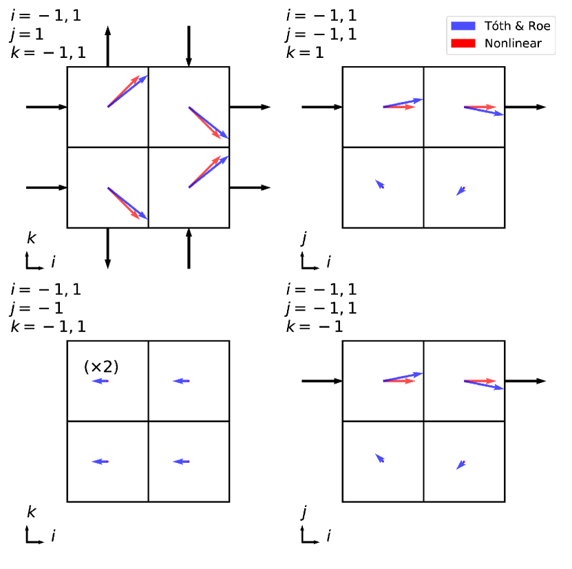
Figure 4: Comparison between the different projections of the interior fields obtained using Tóth & Roe’s operator (blue) and the nonlinear operator here derived (red), from the same exterior fluxes (black) and for a cubic cell. Each panel corresponds to a slice of a coarse cell, for which the indices of the fine cells are given at the upper left (cf. Figure 3). The direction of the original flux is better preserved by the nonlinear operator (cf. right panels), where a component in the $y$-direction that was not originally present appears for the Tóth & Roe operator. The field interpolated using the nonlinear operator is exactly zero for cells with $j=-1$. For clarity, vectors in the lower left panel are represented with a double size.

4.3 Restriction of edge-allocated variables

On each block, magnetic fluxes are updated using the representation of $\mathcal{E}$ correspondent to the level of the block. However, at a fine/coarse interface two different representations of the magnetic flux exist. On the coarse side we have, for example, the magnetic flux $\Phi_{2,0,0}$, while on the fine side, we have $\sum_{i,j=-1,1}\phi_{2,j,k}$. Due to the use of different representations of $\mathcal{E}$ for the update, the two representations of the magnetic flux differ, although in absence of surface monopolar magnetic charge they should coincide. In order to make them consistent without creating divergence on the coarse side, we replace the coarse representation of $\mathcal{E}$ used in the calculation of the circulation with the fine one. To do this, we store both representations of $\mathcal{E}$ on the interface at the time they are calculated. After the time update, we subtract the line integrals of the electric field contained in the interface from the fluxes in contact with it. We then communicate the fine representations to the coarse side and construct a new coarse representation. For example, for an interface at constant $x^{1}$ between a coarse region at the left and a fine region at the right, we replace

$$\mathcal{E}_{2,2,-1}+\mathcal{E}_{2,2,1} \rightarrow\mathcal{E}_{2,2,0}$$

$$\mathcal{E}_{2,-1,2}+\mathcal{E}_{2,1,2} \rightarrow\mathcal{E}_{2,0,2}$$

$$\mathcal{E}_{2,-2,-1}+\mathcal{E}_{2,-2,1} \rightarrow\mathcal{E}_{2,-2,0}$$

$$\mathcal{E}_{2,-1,-2}+\mathcal{E}_{2,1,-2} \rightarrow\mathcal{E}_{2,0,-2}$$

for each coarse cell and recalculate the circulation to update all the fluxes except for $\Phi_{-2,0,0}$. In 2D, no sum is necessary and the coarse representations are simply replaced by the co-spatial fine ones.

4.4 Parallelisation and ghost-cell exchange

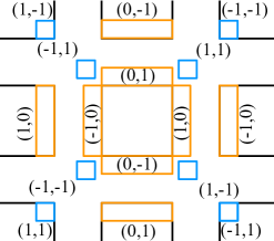
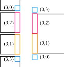
(a)      (b)      (c)

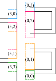
Figure 5: Ghost-cell exchange for blocks (a) at the same resolution level and for coarse/fine interfaces in (b) restriction and (c) prolongation. The numbers represented are the local grid indices to identify neighbours and ghost regions, as explained in Section 4.4. Lines drawn in colour denote (magnetic) fluxes on the boundary faces that are communicated. In panel (c), the dashed lines denote boundaries that contain only tangential fluxes necessary for restriction which reside only on the coarse buffer of a block. The size of fine blocks including ghost regions is marked by a grey line.

To simplify ghost-cell communications in the code, a block’s neighbours and its children are identified by local grid indices $\texttt{i1},\texttt{i2},\texttt{i3}=\{-1,0,1\}$ and local child grid indices $\texttt{ic1},\texttt{ic2},\texttt{ic3}=\{0,1,2,3\}$, both from left (back, bottom) to right (front, top). For example, if block $A$ is directly at the left of block $B$ both belong to the same resolution level, block $A$ is identified as neighbour $(-1,0)$ of block $B$, and block $B$ is identified as neighbour $(1,0)$ of block $A$. This identification strategy is inherited from MPI-AMRVAC (see e.g., Figure 4 of Keppens et al. 2012). When exchanging ghost cells, different array ranges are associated to each index combination, corresponding to the extent of the ghost zones that need to be filled from that neighbour. The identification of neighbours and ghost zones with integer indices allows to easily determine communication patterns using integer arithmetic operations. As an example, Figure 5 shows some of these communication patterns for the case of a two-dimensional grid.

The three panels of Figure 5 show examples of how these local indices are used to identify different ghost regions for (a) same resolution level communications, (b) restriction and (c) prolongation. To ensure that the communicated values are consistent, first same resolution communications are performed, then restrictions and finally prolongations. As in MPI-AMRVAC, to minimise the size of communications at resolution jumps, variables are restricted before being sent and are prolonged after being received. Each block possess a buffer containing a coarse representation of it to facilitate this operations.

In contrast to MPI-AMRVAC, for which inter-processor ghost-cell communications were based on MPI types created using the functions MPI_CREATE_SUBARRAY and MPI_TYPE_COMMIT (see Keppens et al. 2012), BHAC packs all communications, both for staggered and cell centered variables, in one-dimensional arrays using FORTRAN’s reshape function. These buffer arrays are transmitted to other processors using non-blocking MPI communications through the functions MPI_ISEND and MPI_IRECV. When received at the target destination, they are unpacked to fit the shape of the ghost region that they need to fill.

A reason for this change is that the array segments that need to be communicated for each component of the staggered field are different among them and different from those of the cell-centered variables; therefore, using a single buffer instead of a different MPI_TYPE for each of them reduces the number of necessary communications. These and other changes done in the ghost-cell exchange routines are oriented to a future upgrade of the code to a task-based scheduling, which would result in a significant speedup and facilitate the use of hierarchical time-stepping.

Finally, fluxes and electric fields necessary for the consistency steps described in section 4.3 are also written in special communication buffers for sending and receiving. These buffers are likewise one-dimensional arrays filled and extracted using the Fortran reshape function.

4.5 Poles in spherical and cylindrical coordinates

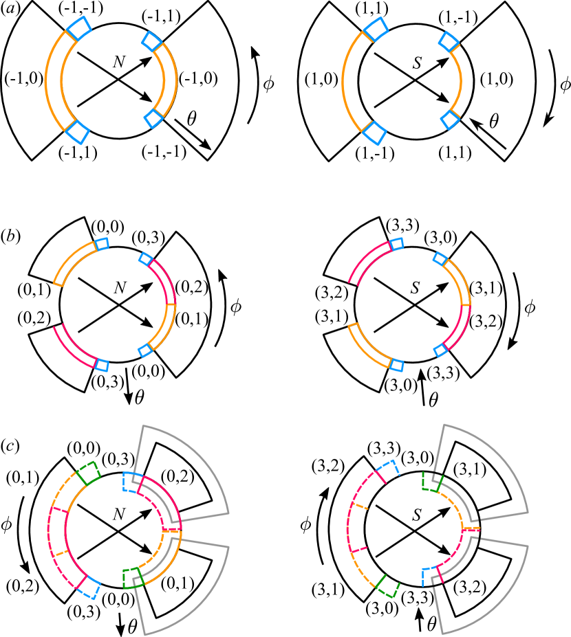
Figure 6: Ghost-cell exchange at the south and north poles in spherical coordinates for same resolution level (a), restriction (b) and prolongation (c). For clarity, the pole is represented as an expanded black circumference to identify the cell faces touching it, although no there is no excised region. As in Figure 5, colored lines denote (magnetic) fluxes on the boundary faces that are communicated. For prolongation, dashed lines denote boundaries that contain only tangential fluxes necessary for restriction and the total extent of fine blocks including ghost regions is marked by a grey line. For cylindrical coordinates, the ghost-cell exchange at the $z$ pole happens as for the north pole.

In three-dimensional simulations in spherical and cylindrical geometry, the ghost-cell exchange at the poles requires special attention. Despite being located at the minimum (and maximum) $\theta$ for spherical and $\rho$ for cylindrical coordinates, in BHAC the pole is not treated as a physical boundary nor it is excised as is usually done in many codes (see e.g.,  Shiokawa et al. 2012). Instead, the connectivity of the blocks touching the poles is changed so that each on them considers as its neighbours the blocks at the opposite side of the polar axis and reconstructions can be performed across the latter.

The only difference respect to the usual ghost-cell exchange is that, after being received, the elements of the receive buffer are reversed in the $\phi$ direction, as is shown in Figure 6. Likewise, periodic boundary conditions such as those in the $\phi$ direction, are handled by changing the connectivity of the grid such that the first block in the $\phi$ direction becomes the neighbour of the last one.

The flux-fixing operation is not necessary at poles, since the areas of cell ‘surfaces’ touching the pole are exactly zero and no flux should be present. Similarly, the contribution of the circulation of the electric field is exactly zero along the polar axis, by recalling that in a coordinate basis $\sqrt{\gamma}$ vanishes there (see equations 20 and 22). Therefore, no fixings are performed and both numerical fluxes and electric fields are set to zero at the pole.

4.6 Boundary conditions

When non-periodic boundary conditions are used, it is necessary to ensure that no divergence is created at boundaries. To accomplish this, we first extrapolate the components of the magnetic field tangential to the boundary according to a user-given prescription, e.g., symmetric, antisymmetric, flat, etc. Then, the normal component is filled layer by layer outwards from the boundary, cancelling the sum of the magnetic fluxes for each cell. For symmetric and antisymmetric boundary conditions, this procedure can be applied without modifications also at resolution jumps; however, this is not the case for flat boundary conditions. The reason is that they consist in copying the value of a variable at the last cell of the physical domain to all of the ghost cells; and in a resolution jump, the sum of two times the last magnetic flux on the fine side is not necessarily equal to the last magnetic flux on the coarse side. Therefore, instead of filling the ghost cells with the values of the last row in the domain, we fill them with an average of the last two rows, weighted by the normal surfaces. In this way, the fine and the coarse representations of the fields at the ghost cells are consistent.

5 Numerical tests

In this section we describe the results of three well known numerical tests performed to validate the new schemes, two in special relativity and one in general relativity. These are the Gardiner & Stone advected magnetic loop (Gardiner & Stone 2005), the cylindrical explosion of Komissarov (1999), and the highly magnetized stationary torus by Komissarov (2006). Since the new additions (CT) and AMR can only be tested in 2D and 3D, and the code has already been validated for 1D problems (see Porth et al. 2017), we omit 1D tests. We also omit tests using both the cell-centred and the staggered variants of arithmetic averaging, except for comparisons with UCT, as the former have already been published in Porth et al. (2017) and Olivares Sánchez et al. (2018).

We are therefore interested in testing the UCT algorithms and the new AMR features, as well as the recently implemented limiters, WENO Z+ and MP5. All of the tests presented here use the equation of state of an ideal fluid with $\hat{\gamma}=4/3$. The prescription for triggering AMR is the Löhner scheme (Löhner 1987), which decides to coarsen or refine based on a quantification of oscillations in the numerical solution.

5.1 Loop advection

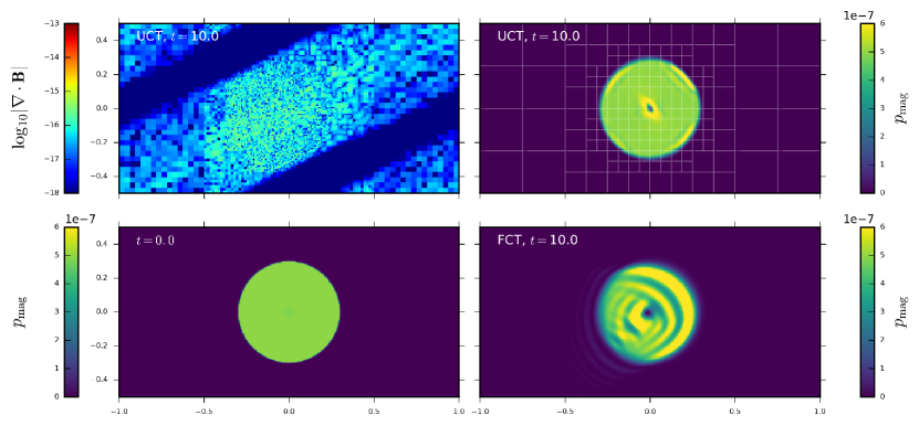
Figure 7: Gardiner & Stone’s loop advection test. Top left: Divergence of the magnetic field after ten time units, using UCT2. Bottom left: Magnetic pressure at the initial configuration. Top right: After ten time units, using UCT2, showing the AMR blocks of $8\times 8$ cells. Bottom right: After ten time units, using flux-CT.

A well known problem to assess the importance of spurious effects due to the divergence-control technique employed in an MHD code is the advection of a weakly magnetized loop. This test was originally used by Gardiner & Stone (2005) to study a divergence-preserving scheme with the upwind property. In this section, we present a comparison of the results obtained using the cell-centered version of flux-CT and the upwind method UCT2.

On a uniform background with $\rho=1$, $p=1$, $v^{x}=0.2$, and $v^{y}=0.1$, the problem consists on advecting a magnetic loop with radius $R=0.3$, described by the potential $A_{z}=A_{0}(R-r)$ for $r\leq R$ and $A_{z}=0$ for $r>R$, where $r^{2}=x^{2}+y^{2}$. $A_{0}$ is chosen $10^{-3}$, so that $\beta=p_{\mathrm{fluid}}/p_{\mathrm{mag}}=10^{6}$ and the loop is advected passively. The domain is $x\in[-1,1]$ and $y\in[-0.5,0.5]$ with periodic boundary conditions. The methods employed are the MP5 limiter, HLLE fluxes and the RK3 time-integrator.

Two realisations of the same set-up are evolved: one using the flux-CT method, and the other UCT2. While for the former it is not possible to use AMR, for the latter three levels of AMR are used. The highest AMR-level has a resolution equivalent to that of the flux-CT run, i.e, $256\times 128$.

The magnetic pressure at the initial condition and some snapshots of the evolution are depicted in figure 7. The upper-left panel of the same Figure shows the divergence of the magnetic field for the UCT2 run at the final time $t=10.0$, when the magnetic loop, and thus the refined region, has travelled a complete cycle across the domain. Divergence remains always zero at machine precision ($\sim 10^{-16}$) despite resolution jumps and coarsening/refining of blocks. It can be seen that, in addition to the AMR capacity, the staggered UCT scheme is able to preserve much better the original shape of the loop, without creating as many spurious oscillations as flux-CT.

5.2 Cylindrical explosion

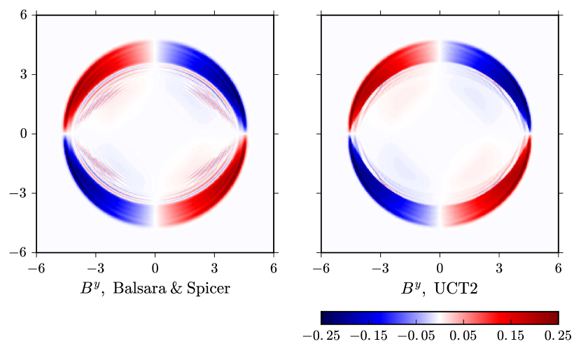
Figure 8: Cylindrical explosion. $y$-component of the magnetic field at $t=4.0$ when using the BS algorithm (left) and UCT2 (right)

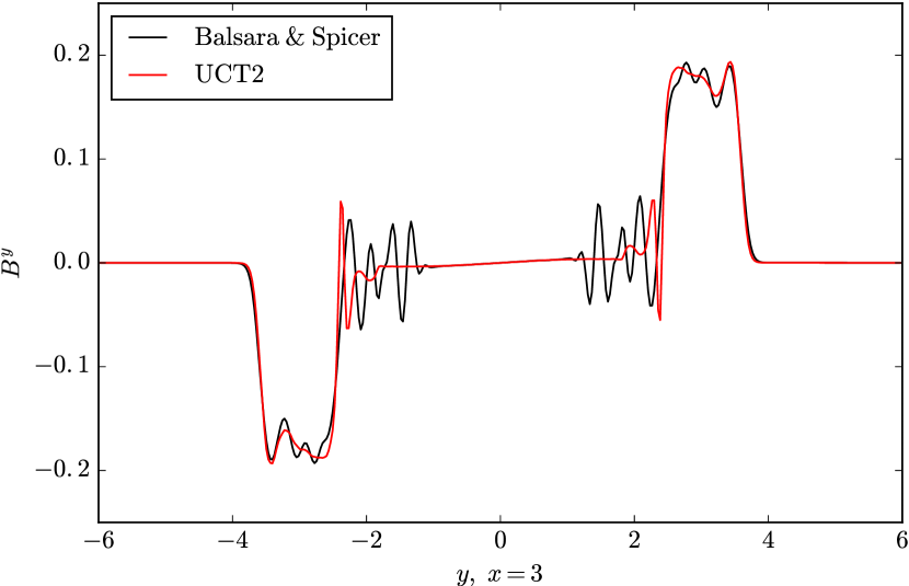
Figure 9: Cylindrical explosion. Profile of the $y$-component of the magnetic field along a line at $x=3$. The Balsara & Spicer algorithm shows a more oscillatory behavior as compared with UCT2.

Another challenging problem for MHD codes is that of a cylindrical blast wave expanding in a homogeneous plasma with an initially constant magnetic field. We present results of such problem, which highlights the importance of upwinding in the calculation of electric fields, and show the different behavior of the BS and the UCT2 schemes. The problem set-up is the same that appears in Del Zanna et al. (2007) and Komissarov (1999).

The domain extends over $[-6,6]\times[-6,6]$. Plasma is initially at rest, with a constant magnetic field $B^{x}=0.1$, $B^{y}=B^{z}=0$. Defining $r^{2}=x^{2}+y^{2}$, the domain is divided in three regions: a high density and pressure ($\rho_{\mathrm{in}}=10^{-2}$, $p_{\mathrm{in}}=1$) region for $r<r_{\mathrm{in}}=0.8$, a low density and pressure ($\rho_{\mathrm{out}}=10^{-4}$, $p_{\mathrm{out}}=5\times 10^{-4}$) region for $r>r_{\mathrm{out}}=1.0$, and a transition region for $r_{\mathrm{in}}\leq r\leq r_{\mathrm{out}}$ where $\rho=\rho_{\mathrm{in}}(r/r_{\mathrm{in}})^{\alpha_{1}}$ and $p=p_{\mathrm{in}}(r/r_{\mathrm{in}})^{\alpha_{2}}$, and the exponents $\alpha_{1}$ and $\alpha_{2}$ are such that $p(r)$ and $\rho(r)$ are continuous at $r_{\mathrm{in}}$ and $r_{\mathrm{out}}$. The boundary conditions are periodic, although this is not relevant in practice, since the region of interest cannot be affected by signals coming form the boundaries during the simulation time.

The system is evolved until $t=4.0$ with an RK3 integrator and a CFL factor of 0.35, and HLLE fluxes with WENOZ+ reconstruction are used. The simulation used three AMR levels, with a base resolution of $100\times 100$, giving an effective resolution of $400\times 400$. To compare the two algorithms for magnetic-field evolution, we run two simulations, one using the BS algorithm and the other using UCT2.

Figure 8 shows the last snapshot of the evolution for both methods. Spurious oscillations behind the reverse shock are more pronounced for the BS method, similar to those already encountered in Section 5.1.

The situation greatly improves when adopting the UCT2 algorithm, as can be further confirmed by examining the profiles of the $y$-component of the magnetic field along the line $x=3$ shown in Figure 9.

5.3 Stationary torus

The test presented in this section is the analytic solution found by Komissarov (2006) for an equilibrium torus with a toroidal magnetic field. As in Porth et al. (2017), the implementation of the initial condition in BHAC is based on routines kindly provided by Chris Fragile. Taking advantage of the stationarity of this analytic solution, we use this test to quantify the convergence of the numerical solution. Recalling the results from Komissarov (2006), for a fluid of constant angular momentum distribution $l=-u_{\phi}/u_{t}=l_{0}$, and adopting a specific relation of the fluid and magnetic pressure with respect to the fluid enthalpy, the configuration is described by the equation

$$\mathcal{W}-\mathcal{W}_{in}=-{\kappa\over\kappa-1}{p\over\rho h}-{\eta\over\eta-1}{p_{m}\over\rho h}\,,$$ (41)

where $\mathcal{W}=\ln|u_{t}|$ and $\kappa$ and $\eta$ are constants. To completely specify the solution, it is necessary to give two more parameters, namely the fluid enthalpy and the ratio of fluid to magnetic pressure at the centre of the torus, $(\rho h)_{c}=\omega_{c}$ and $(p/p_{\rm mag})_{c}=\beta_{c}$, respectively. The parameters of the torus chosen here as a test problem are $\kappa=4/3$, $\eta=4/3$, $l_{0}=2.8$, $r_{c}=4.62$, $\mathcal{W}_{in}=-0.030$, $\omega_{c}=1.0$, and $\beta_{c}=0.1$. The dimensionless spin of parameter of the black hole is set to $a=0.9$, and the plasma follows the equation of state of an ideal fluid with $\hat{\gamma}=4/3$. Simulations are performed in 3D and using logarithmic Kerr-Schild coordinates (i.e., MKS coordinates with ${\vartheta_{0}}=0$ and $R_{0}=0$). The simulation domain spans over $\theta\in[\pi/5,4\pi/5]$, $r_{\rm KS}\in[0.95\,r_{\mathrm{h}},\ 50\,M]$ and $\phi\in[0,\pi]$, where $r_{\rm KS}$ is the radial Kerr-Schild coordinate and $r_{\mathrm{h}}$ is the (outer) event horizon radius of the BH. To test convergence, we performed three simulations progressively doubling the resolution from a base grid of $N_{r}\times N_{\theta}\times N_{\phi}=100\times 60\times 40$. The rotation period of the center of the torus is $68\,M$, and the simulation is carried out until $t=100\,M$, thus spanning nearly one and a half orbital periods. Although this kind of solutions are known to be unstable to the MRI and the Papaloizou-Pringle instability in 3D (Wielgus et al. 2015; Bugli et al. 2018), the time elapsed by our simulations still corresponds to the initial phase of the linear growth, and no chaotic behaviour can be observed. In fact, the torus here presented is identical to Case A simulated by Wielgus et al. (2015), who reported perturbations at $t=100\ M$ still at the $\sim 10^{-4}$ level.

To emulate vacuum regions outside the torus, a tenuous atmosphere with density and pressure given by $\rho=\rho_{\mathrm{min}}\,r_{\rm KS}^{-3/2}$, $p=p_{\mathrm{min}}\,r_{\rm KS}^{-5/2}$ with $\rho_{\mathrm{min}}=10^{-5}$ and $p_{\mathrm{min}}=10^{-7}$ was added. Initially, the velocity of the atmosphere is set to zero in the Eulerian frame. However, the atmosphere is free to evolve, and only density and pressure are reset to the atmosphere value whenever they fall below it. The numerical methods chosen for this test were the HLLE Riemann solver, LIMO3 reconstruction and two-step time integration with CFL factor $0.5$.

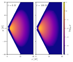
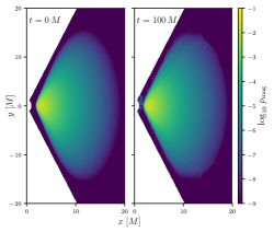
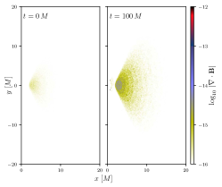
Figure 10: Rest mass density, plasma beta and divergence of the magnetic field at $t=0$ and $t=100$ for the run with $N_{r}=400$ of the Komisssarov torus test.

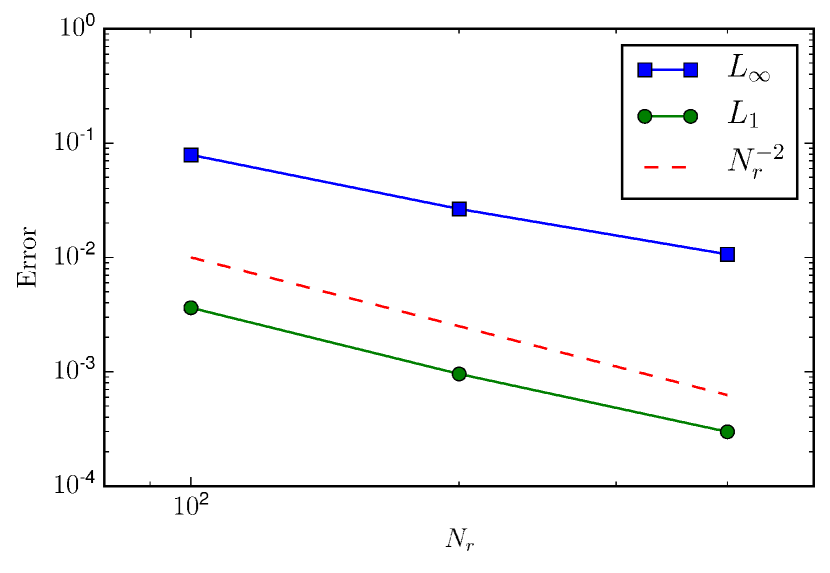
Figure 11: $L_{\infty}$ and $L_{1}$ norms of the error in density $\rho$ for the strongly-magnetised Komissarov torus at $t=70\,M$, i.e., after one orbital period. The scheme shows second order convergence.

Fig. 10 shows the density distribution, the plasma beta and the divergence of the magnetic field at the initial state and at $t=100\,M$ for the run with resolution $N_{r}=400$. As can be seen, the distribution of the displayed quantities is very well preserved by the scheme. The $L_{1}$ and $L_{\infty}$ errors (calculated by comparing with the last state with the initial condition) are shown in Figure 11. Consistently with the algorithm employed, second order convergence can be observed.

6 Magnetized black-hole accretion

In this section we present simulations where the newly implemented numerical methods are applied to evolve the accretion of plasma onto black holes, one of the main target applications of the code.

In Porth et al. (2017), simulations of this kind, performed at uniform resolution, were used to validate the code by means of qualitative and quantitative comparisons with the widely used GRMHD code HARM (Gammie et al. 2003; Noble et al. 2009). Therefore, this section will be focused in showing the advantages of AMR and the effects of the choice of divergence control technique.

For all the simulations in this section, the initial configuration is a torus in equilibrium around a black hole (Fishbone & Moncrief 1976) with spin parameter $a=0.9375$, and thus with the outer event horizon located at $r=1.348\,M$, where $r$ is the radial Kerr-Schild coordinate. The inner radius of the torus is at $r_{\mathrm{in}}=6\,M$, and its density maximum at $r_{\mathrm{max}}=12\,M$ (orbital period of $247\,M$ at the density maximum). The density in the torus is normalized so that it takes 1.0 as its a maximum value. A single-loop poloidal magnetic field is built from the vector potential $A_{\phi}\propto{\rm max}(\rho/\rho_{\rm max}-0.2,0)$ and is normalized in such a way that the highest magnetic pressure and the highest thermal pressure are related by the ratio $\beta=p_{\mathrm{fluid,max}}/p_{\mathrm{mag,max}}=100$. To break this equilibrium state, random perturbations of $4\%$ are added to the pressure. This eventually triggers the MRI, allowing the plasma to accrete. It is worth mentioning that even without explicitly adding a perturbation, numerical errors produced by the discretization would be amplified to produce a turbulent state very similar to that obtained. However, in order to have some control on the initial state, the perturbation we add is significantly larger than numerical errors (which are not easily predictable) but still small respect to the equilibrium pressure. In addition, since the initial growth rate of the perturbation depends on its amplitude, the saturated state can be reached faster with larger perturbations. For this reason, starting with seed perturbations is computationally less expensive than waiting for the initial discretization errors in the equilibrium state to grow. Moreover, the value of $4\%$ is the same used in Porth et al. (2017), and is therefore useful for making comparisons.

To avoid vacuum regions, the rest of the simulation is filled with a tenuous atmosphere with density $\rho_{\mathrm{fl}}=10^{-4}r^{-3/2}$ and fluid pressure $p_{\mathrm{fl}}=1/3\times 10^{-6}\ r^{-5/2}$. We reset the density or the pressure whenever they fall below these floor values. Simulations were evolved using a two-step time-integrator.

As mentioned in Section 2.2, several coordinate systems for black-hole spacetimes are available in BHAC. The simulations shown here are performed in MKS, as well as in CKS coordinates. Both coordinate systems possess advantages and weaknesses that must be taken into account depending on the aspect of the physical system under study, as will be explained below. The simulations whose results are reported in this section are summarised in table 2.

6.1 2D MKS simulations

The first pair of simulations is performed in 2D on the meridional plane. The domain covers $\theta\in[0,\pi]$ and $r\in[1.2,2500]$, and is resolved using three AMR levels triggered by the Löhner scheme, with a base resolution of $N_{r}\times N_{\theta}=200\times 100$ and an effective resolution of $N_{r}\times N_{\theta}=800\times 400$. Since the time step for these 2D simulations is not penalised by the small width of cells in contact with the polar axis, the parameter ${\vartheta_{0}}$ of MKS coordinates is set to zero. Reconstruction is performed using PPM. The purpose of these two simulations is to investigate the effect of the method utilised for the evolution of the magnetic field; therefore, the only difference between them was the use of either the Balsara & Spicer algorithm or UCT2.

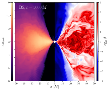
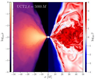
Figure 12: Comparison between 2D simulations of black-hole accretion using the Balsara & Spicer method (left) and the UCT2 algorithm (right) at $t=5000\,M$. For each panel, rest mass density $\rho$ is shown at the left and plasma $\beta$ at the right.

A comparison at $t=5000$ (Figure 12) displays what we observe to be systematic differences between the two simulations. Namely, a higher magnetisation inside the funnel for the UCT2 run and a different morphology of the jet, which acquires a parabolic shape for the Balsara & Spicer run and is more conical for the UCT2 run. Another difference lays in the transition between the funnel and the mildly magnetized wind surrounding the jet, which is sharper for the UCT2 case. These differences could have important observational consequences, for instance, in future high-resolution VLBI images of the SMBH candidates in M 87 and Sgr A*, since radiative models of these sources which are able to reproduce the properties of their radio spectrum consider that most of the radio emission originates at the funnel wall (Mościbrodzka et al. 2016).

From these simulations, it is possible to see that the choice of method for evolving the magnetic field can have a visible effect on the flow behavior. Among these two methods, we would recommend the use of UCT2 due to its upwind properties and to the possibility of using high-order reconstructions. Although some asymmetry respect to the equator can be seen in both the BS and the UCT2 simulations, this is only a consequence of the chaotic evolution of the initial random perturbations driven by turbulence, and not of the numerical schemes. Even though not included in the tests presented in this work, in order to verify that the scheme does not possess any directional bias, we have simulated the development of the magnetic Kelvin-Helmholtz instability with a controlled perturbation (Tóth & Roe 2002) and employing the same methods (PPM and BS or UCT2). When comparing with a simulation starting from an initial condition obtained by specular reflection, we obtained identical results. Finally, it is worth mentioning that the simulation using the Balsara & Spicer method was tested previously against another run performed in an equivalent uniform resolution and using the widespread flux-CT method. The AMR run was able to achieve a speedup factor of 7.1, while obtaining quantitatively similar results in the mass accretion rate and the magnetic flux through the horizon, as discussed in Olivares Sánchez et al. (2018).

6.2 3D MKS simulations

Since self-sustaining dynamo activity leading to the perpetuation of the MRI cannot occur in strict azimuthal symmetry (Cowling 1933; Balbus & Hawley 1991), 3D simulations are necessary to study the accretion flow in the saturated state.

The AMR capabilities of the code become even more important in this case, where the computational cost of simulations rapidly increases due to the larger number of computing cells. In addition, the polar coordinate system naturally leads to a significantly higher resolution close to the polar axis, which is not always justified, and the narrow cells in these regions usually cause a penalisation in time-step size.

A possibility to alleviate this limitation is to de-refine cells close to the polar axis, as done by White et al. (2016). In typical accretion scenarios, the polar region is occupied by an evacuated, smooth funnel, thus no especially high resolution is required. In contrast, equatorial regions are populated by turbulent structures that need to be properly resolved.

Newtonian shearing box simulations have shown that an insufficient resolution can suppress the growth of the MRI when the wavelength of its fastest growing mode $\lambda_{\rm MRI}$ is resolved with less than six cells, and move the simulation away from the ratio of magnetic to gas pressure expected at the saturated state (Sano et al. 2004). A relativistic version of this criterion has been applied to estimate whether global accretion simulations are properly resolved (see e.g.,  Noble et al. 2010; McKinney et al. 2012).

The MRI quality factor is defined as the ratio between the grid spacing and $\lambda_{\mathrm{MRI}}$, which approximately gives the number of cells employed to resolve it. Following Noble et al. (2010), we define the relativistic MRI quality factor as

$$Q^{(i)}_{\rm MRI}=\frac{\lambda^{(i)}_{\rm MRI}}{\Delta x^{(i)}}=\frac{2\pi}{\Omega}\frac{|b^{(i)}|}{\Delta x^{(i)}\sqrt{\rho h+b^{2}}}\,,$$ (42)

where $b^{(i)}$ and $\Delta x^{(i)}$ are, respectively, the magnetic field and the displacement in the $i$-th direction in the orthonormal frame co-moving with the fluid, and $\Omega$ is the orbital angular velocity. Since the value of $b^{(i)}$ depends on the amplification of the magnetic field experienced during the simulation, $Q^{(i)}_{\rm MRI}$ can only be determined a posteriori. For a fluid rotating in the $\phi$ direction, $Q^{(\theta)}_{\rm MRI}$ is the relevant MRI quality factor.

The simulation presented in this section, labelled as MKS192-UCT (see table 2), is performed on a static grid that has been de-refined at the poles. More specifically, the AMR blocks touching both the polar axis and the inner radial boundary, which contain the smallest cells and therefore determine the global time-step, were forced to the coarsest refinement level. In addition to the settings described at the beginning of this section, the simulation domain spans $r=[1.18\,M,10000/3\,M]$ and the extent in $\theta$ and $\phi$ subtends the whole $4\pi$ steradians solid angle. The resolution at the base level is $N_{r}\times N_{\theta}\times N_{\phi}=128\times 48\times 48$, and the simulation contains 3 AMR-levels, giving an effective resolution of $512\times 192\times 192$ cells. As an additional measure to prevent the time-step penalisation from the poles, this time the MKS ${\vartheta_{0}}$-parameter is set to 0.25.

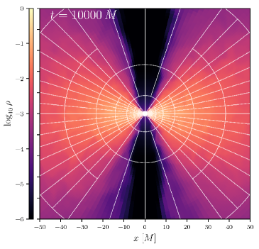
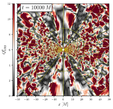
Figure 13: Logarithmic rest-frame density (left panel) and MRI quality factor (right panel) for simulation MKS192-UCT, showing the AMR blocks of $N_{r}\times N_{\theta}\times N_{\phi}=32\times 8\times 8$ cells each. The grid is able to concentrate resolution in the disk in order to achieve $Q^{(\theta)}_{\rm MRI}>6$ in the torus, as recommended in Sano et al. (2004), while saving computational costs by de-refining the polar regions.

Figure 13 shows a snapshot of simulation MKS192-UCT at $t=10\,000\,M$. The AMR blocks, of $32\times 8\times 8$ cells each, are drawn in white lines. The left panel of that figure shows the logarithm of density, while the right panel shows the MRI-quality factor. It can be observed that the simulation grid is able to maintain $Q^{(\theta)}_{\rm MRI}>6$ in the disk without requiring a similarly high resolution at the polar regions, which are occupied by a smooth low-density outflow and where MRI-driven angular momentum transport does not play an important role. It is necessary to keep in mind that places where $Q^{(\theta)}_{\rm MRI}\sim 0$ within the disc correspond to regions where the magnetic-field changes sign (see Eq. 42).

As can be seen in Figure 14, the mass-accretion rate $\dot{M}$ and magnetic flux through the horizon $\Phi_{\rm BH}$ (Tchekhovskoy et al. 2011) are consistent with those from the highest resolution of Porth et al. (2017) (labelled here as MKS192-fCT, see table 2), which used the same initial condition and the numerical methods validated in that work including the flux-CT scheme. In both cases, the behavior consists of a transient growth ($t<\leavevmode\nobreak\ 5000\,M$) followed by a quasi-stationary state after the saturation of MRI ($t>\leavevmode\nobreak\ 5000\,M$).

As an additional comparison tool, we compute time- and disk-averaged profiles similar to those shown in Beckwith et al. (2008); Shiokawa et al. (2012); White et al. (2016); Porth et al. (2017). For a quantity $q(t,x^{i})$, these averages are defined as

$$\langle q\rangle=\frac{\int_{t_{\rm min}}^{t_{\rm max}}\int_{\theta_{\rm min}}^{\theta_{\rm max}}\int_{0}^{2\pi}\sqrt{-g}\ q(t,r,\phi,\theta)\ d\phi\ d\theta\ dt}{\int_{t_{\rm min}}^{t_{\rm max}}\int_{\theta_{\rm min}}^{\theta_{\rm max}}\int_{0}^{2\pi}\sqrt{-g}\ d\phi\ d\theta\ dt}\,,$$ (43)

were $\theta_{\rm min}=\pi/3$, $\theta_{\rm min}=2\pi/3$, $t_{\rm min}=5000\,M$ and $t_{\rm min}=10000\,M$.

As shown in Figure 15, the averaged profiles of MKS192-UCT show a reasonable quantitative agreement with those of MKS192-fCT, despite the use of different methods and resolution. It should be noted, however, that the angular resolution in theta, which is essential to capture the MRI, is effectively the same for the two simulations performed in MKS coordinates, due to the use of three AMR levels in the former. As will be shown in Section 6.3, a better agreement is found with simulation CKS8-UCT, which employs CKS coordinates, with differences arising from well understood reasons. The fact that such a better agreement can be found between simulations using different coordinate systems, and thus completely different spatial discretizations, shows that the differences between MKS192-fCT and MKS192-UCT are likely more a consequence of the method employed to evolve the magnetic field rather than of the slightly different radial resolution.

Simulation	Coordinates	Domain $[M]$	AMR levels	Base resolution	$\boldsymbol{B}$-evolution
2DMKS-BS	MKS	$[1.2,2500]$	3	$200\times 100$	BS
2DMKS-UCT	MKS	$[1.2,2500]$	3	$200\times 100$	UCT2
MKS192-fCT	MKS	$[1.2,2500]$	1	$384\times 192\times 192$	flux-CT
MKS192-UCT	MKS, ${\vartheta_{0}}=0.25$	$[1.2,1000/3]$	3	$128\times 48\times 48$	UCT2
CKS8-UCT	CKS	$x,y\in[-500,500]$	8	$96\times 96\times 192$	UCT2
		$z\in[-1000,1000]$

Table 2: A summary of the simulations referred to in Section 6. When not specified, the MKS parameters $R_{0}$ and ${\vartheta_{0}}$ are zero. The base grid resolution is displayed as $N_{r}\times N_{\theta}(\times N_{\phi})$ for the MKS simulations and as $N_{x}\times N_{y}\times N_{z}$ for the CKS.

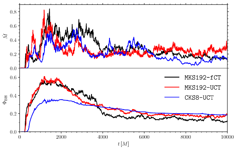
Figure 14: Mass-accretion rate (top) and magnetic flux through the horizon (bottom) for the 3D simulations shown in this work in MKS and CKS coordinates using UCT2 (see table 2), and for the highest-resolution simulation in MKS coordinates shown in Porth et al. (2017), using flux-CT.

6.3 3D CKS simulations

Despite the strategies to avoid slow time steps from polar regions described in Section 6.2 and the self-consistent treatment of poles by rearranging the grid topology described in Section 4.5, the poles of a coordinate system still represent an inhomogeneity in the numerical domain that could in principle introduce artefacts or a directional bias in the simulation.

In addition, although logarithmic grids in polar coordinates ensure machine-precision conservation of angular momentum and are very efficient at resolving small-scale features when the interesting dynamics occur near the origin, they loose resolution far away from it.

Therefore, in order to study systems that are extended in space and for which an artificial directional bias could be misinterpreted as a physical property of the system, it might be useful to resort to coordinate systems that are more spatially homogeneous. An obvious choice are coordinate systems based on Cartesian coordinates, which are often used for GRMHD simulations in full general relativity (see e.g.,  Giacomazzo & Rezzolla 2007; Etienne et al. 2015). However, the necessity to properly resolve the black-hole horizon and the MRI renders large scale ($\sim 10^{3}\ r_{g}$) simulations impossible, unless some form of mesh refinement is used.

In this section we present a simulation performed in CKS coordinates, labelled as CKS8-UCT in Table 2. A combination of AMR and static mesh refinement is used to ensure sufficient resolution at the black-hole horizon and the MRI turbulence while following the jet with dynamic mesh refinement.

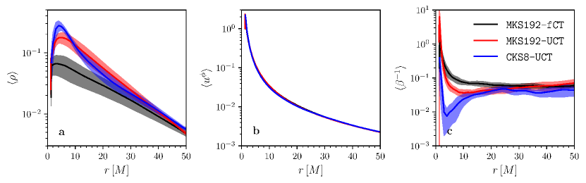
Figure 15: Disk- and time-averaged profiles of rest mass density (a), $\phi$-component of the 4-velocity (b), and inverse plasma $\beta$ (c), in the interval 5000-10000 $M$, for the 3D simulations of magnetized accretion referred to in this work (see table 2). Shaded regions show the standard deviation from the average value for each simulation. (These are, however, hardly noticeable for $u^{\phi}$ due the small standard deviation and the excellent agreement between the three curves.) After taking into account the different numerical methods and coordinates employed, the three simulations show reasonably consistent profiles, with the deviations in density and plasma $\beta$ at $r_{KS}<10\ M$ for simulation CKS8-UCT probably caused by a poor resolution of the MRI in that region (see also Figure 16).

The domain is structured as a set of nested boxes for which a different maximum refinement level is specified. The highest AMR level can be reached only by the innermost box, which contains the black-hole horizon. In order to follow the jet dynamics, refinement is triggered by variations in the plasma magnetisation $\sigma=b^{2}/\rho$ and the density $\rho$, using the Löhner scheme. In order to limit the overhead by alternating refinement and de-refinement of the same regions, re-gridding is performed only every 1000 iterations (since hierarchical time-stepping has not yet been implemented in BHAC, these correspond to the time-step of the finest grid). The simulation employs 8 AMR levels, with a base resolution of $N_{x}\times N_{y}\times N_{z}=96\times 96\times 192$, and extending over $x,y\in[-500\,M,500\,M]$, and $z\in[-1000\,M,1000\,M]$. The magnetic field is evolved using the UCT2 algorithm. In order to prevent an unphysical outflow from the black-hole interior, we apply cut-off values for the density and pressure in the region $r<0.5(r_{\rm H-}+r_{\rm H+})$, where $r_{\rm H-}$ and $r_{\rm H+}$ are the location of the inner and outer event horizons. In particular, we set $\rho_{\rm cut}=10^{-2}$ and $p_{\rm cut}=10^{-4}$.

Figure 16 displays different cuts of the simulation at $t=10000\ M$. The two left panels are horizontal cuts at $z=100\ M$ (panel a) and $z=0$ (panel b), and the right panel is a vertical cut at $y=0$ (panel c). In panel (a) it is possible to appreciate a cross-section of the jet, which is now completely free to wobble and to change shape independently of the coordinate surfaces. Panel (c) shows the automated mesh refinement following the evolution of the jet, indicated by a high plasma magnetisation $\sigma=b^{2}/\rho$, as it propagates in the $\pm z$ direction. Also in this panel it can be noticed that the shape of the jet does not appear constrained by the coordinate surfaces. In a future work we will provide a more detailed comparison of the jet dynamics in simulations using Cartesian and spherical grids.

At the same time as the jet is resolved with such detail, panel (b) shows that in most of the disk MRI is resolved with high quality factors, being the only exception the region for which $r_{\rm KS}<10\ M$.

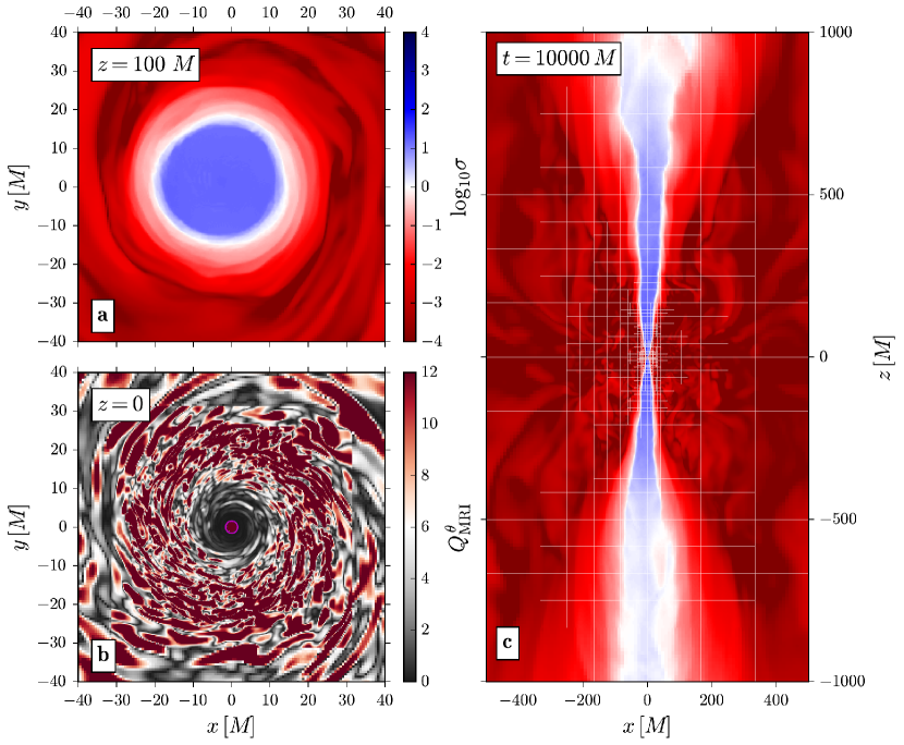
Figure 16: Cuts of the simulation CKS8-UCT (see Table 2) at $t=10000\ M$, showing logarithmic plasma magnetisation $\sigma=b^{2}/\rho$ and MRI quality factor in the $\theta$-direction, $Q^{(\theta)}_{\rm MRI}$. Panel a: Cross section of the jet at $z=100\ M$. Panel b: MRI-quality factors in the disk at $z=0$. A magenta circumference marks the black-hole outer horizon. Panel c: AMR blocks, of $16^{3}$ cells, following the propagation of the jet.

To quantitatively compare the results of this Cartesian simulation with those presented in the previous sections, also in this case we compute the mass-accretion rate and magnetic flux through the horizon as well as time- and disk-averaged profiles in the same intervals as mentioned in Section 6.2.

In Figure 14, the mass-accretion rate shows a remarkably consistent behavior for all of the three simulations, with variations being a consequence of the turbulent nature of the process. On the other hand, the absolute magnetic flux through the horizon, though overall consistent in magnitude, shows significantly less variations for the Cartesian case. This is accompanied by a smaller maximum in the initial transient growth. This could likely be attributed to a poorer resolution of the disk region which hinders magnetic-field amplification due to MRI. In fact, although overall high quality factors are obtained within the disk, the decrease in $\lambda^{(\theta)}_{\rm MRI}$ due to the density increase close to the black hole is not accompanied by a corresponding increase in resolution as is the case for spherical polar coordinates (cf. panel b of Figure 16 and right panel of Figure 13). A more adequate resolution could be achieved by allowing higher AMR levels in this region.

The averaged profiles shown in Figure 15 are as well in good agreement with the other 3D simulations, especially with MKS192-UCT, which employs the same algorithm to evolve the magnetic field. The agreement is practically perfect for the $\phi$-component of the 4-velocity in all three simulations and it remains mostly within one standard deviation between simulations CKS8-UCT and MKS192-UCT. The most important deviations in density and plasma $\beta$ at $r_{\rm KS}<10\ M$ with respect to MKS192-UCT could likely be attributed to the poorer resolution of MRI in that region, which hinders the amplification of the magnetic field and the angular momentum transport leading to an accumulation of mass in that region. In fact, panel (c) of Figure 15 is consistent with a result from Sano et al. (2004), namely that a poor resolution leads to values of the magnetic pressure (and thus of $\beta^{-1}$) smaller than those expected at the saturation of MRI.

Finally, Table 3 lists several properties of runs CKS8-UCT and MKS192-UCT at the end of the simulation, related to how well they can resolve physics. These are: number of cells resolving the horizon, total cell population, time-step and average volume of occupied cells, i.e., the average proper volume of cells which contain matter coming from the disk, which is identified by a passively advected tracer. Unsurprisingly, it can be seen that, although MKS simulations are able to resolve better the horizon and reach higher MRI quality factors in the disk region, overall the domain is more resolved in the CKS case. As a consequence, simulations in Cartesian coordinates could be useful to study the large-scale effects on the jet produced by finer features arising from Kelvin Helmholtz or kink instabilities, as those visible in Figure 16.

Furthermore the small sizes of cells close to the polar axis or the outer event horizon produces a penalisation in time-step for MKS simulations which is absent for the Cartesian case, which is thus able to advance more physical time per iteration. However, the price to pay for a more resolved domain in the latter is a much larger cell population which currently is updated simultaneously, significantly increasing the computational cost of these simulations. In the future, this limitation will be overcome to some extent by adopting a hierarchical time step as is done in several AMR-codes (see e.g.,  Cunningham et al. 2009; Liska et al. 2018).

In summary, due to the advantages mentioned above, Cartesian adaptive meshes appear as a very interesting resource to study large-scale jet propagation in simulations which self consistently include the jet engine, as well as other systems for which no symmetry is to be assumed a priori, as tidal disruption events or precessing disks. Currently, the Cartesian simulation described above is being used to model the appearance of the jet-launching region in M 87 (Davelaar et al. 2019).

Simulation	$N_{\rm H}$	$\langle\Delta V\rangle_{\rm occ}^{\frac{1}{3}}$	$N_{\rm cells}$	$\Delta t$
CKS8-UCT	$2\,880$	2.9	70 811 648	$2.44\times 10^{-2}$
MKS192-UCT	$20\,736$	7.6	6 144 000	$4.71\times 10^{-3}$

Table 3: Comparison between Cartesian and spherical runs for the same accretion problem. The quantities shown are: number of cells resolving the outer event horizon $N_{\rm H}$, cubic root of the average proper volume per occupied cell, total cell population and time step, with all quantities measured at time $t=10000\ M$.

7 Conclusion

We described in detail new additions to the GRMHD code BHAC, namely three CT algorithms based on staggered meshes, as well as AMR strategies compatible with them. The variants of CT implemented in BHAC are the arithmetic average of Balsara & Spicer (1999) (BS) and the two upwind schemes by Londrillo & Del Zanna (2004) and Del Zanna et al. (2007) (UCT), which allow the use of high-order reconstructions.

In order for the divergence of the magnetic field to be zero to machine precision across coarse/fine boundaries and during the creation and destruction of blocks caused by AMR, special divergence-preserving restriction and prolongation operators are required. We derived and employ a class of such operators that generalises those obtained for Cartesian geometry by Tóth & Roe (2002). In addition, we presented technical information on the data structures used, the ghost-cell exchange which was re-designed for staggered variables, and the treatment of the poles in spherical and cylindrical coordinates, as well as on divergence-preserving boundary conditions.

We validated these new additions by showing the results of tests commonly used in the community, specifically, Gardiner & Stone (2005)’s loop advection test and the cylindrical explosion from Komissarov (1999) in special relativity, and the magnetised stationary torus from Komissarov (2006) in general relativity. We observed that, in agreement with analogous tests present in the literature, UCT methods generate less spurious oscillations than the flux-CT and BS methods, both still widely used in GRMHD and MHD codes, and that the algorithm converges at the expected rate.

By performing 2- and 3-dimensional simulations of magnetized accretion onto a black hole, we could notice that the BS method can give different results in physically relevant problems as compared to UCT methods. Due to its upwind properties and to the possibility of employing high-order reconstructions in UCT methods, we decided to use the latter schemes for future simulations. In addition, we showed that the code’s AMR capabilities can be exploited in black hole accretion simulations in order to eliminate the penalisation in time-step caused by the small width of the cells around the pole in spherical coordinates, while maintaining an optimal resolution at the turbulent equatorial regions.

As an example of a problem inaccessible, or at least extremely expensive for non-AMR codes, which can be performed using the new capabilities added to the BHAC infrastructure, we simulated black-hole accretion in Cartesian Kerr-Schild coordinates. The use of a Cartesian mesh could permit the study of jet dynamics including self consistently the black-hole engine, while avoiding any possible directional bias introduced in the mesh by the presence of a polar axis. Furthermore, AMR can be used to accurately simulate magnetohydrodynamical instabilities between the disk wind and the jet occurring during its propagation, making similar set-ups extremely useful for self-consistently modelling sources such as M 87 (Davelaar et al. 2019) and Cen A (Fromm et al. 2019), as will be shown in future work. As mentioned before, Cartesian coordinates and AMR could be very useful also in accretion scenarios without symmetries, such as tidal disruption events or precessing disks.

Recent developments in the code that will be presented as well in forthcoming publications include an accurate modelling of electron thermodynamics (Mizuno 2019) and the addition of a module for resistive GRMHD (Ripperda et al. 2019) which also employs the staggered grid infrastructure developed in the present work. A set of comprehensive tests showing consistency between results obtained with several state-of-the-art GRMHD codes including BHAC for the same accretion problem will be presented in Porth et al. (2019).

All of these tools, together with the current capabilities of BHAC, are meant to contribute to a detailed modelling of strong-field field phenomena in astrophysics, which is becoming increasingly relevant for international efforts such as the EHT and BlackHoleCam (Event Horizon Telescope Collaboration et al. 2019a, b, c, d, e, f).

References

- Abdujabbarov et al. (2015) Abdujabbarov, A. A., Rezzolla, L., & Ahmedov, B. J. 2015, Mon. Not. R. Astron. Soc., 454, 2423
- Acker et al. (2016) Acker, F., B. de R. Borges, R., & Costa, B. 2016, J. Comput. Phys., 313, 726
- Akiyama et al. (2015) Akiyama, K., Lu, R.-S., Fish, V. L., et al. 2015, Astrophys. J., 807, 150
- Alcubierre (2008) Alcubierre, M. 2008, Introduction to Numerical Relativity (Oxford, UK: Oxford University Press)
- Aloy & Rezzolla (2006) Aloy, M. A. & Rezzolla, L. 2006, Astrophys. J., 640, L115
- Anile (1990) Anile, A. M. 1990, Relativistic Fluids and Magneto-fluids (Cambridge, UK: Cambridge University Press)
- Anninos et al. (2017) Anninos, P., Bryant, C., Fragile, P., et al. 2017, The Astrophysical Journal Supplement Series, 231, 17
- Anninos et al. (2005) Anninos, P., Fragile, P. C., & Salmonson, J. D. 2005, Astrophys. J., 635, 723
- Antón et al. (2006) Antón, L., Zanotti, O., Miralles, J. A., et al. 2006, Astrophys. J., 637, 296
- Baiotti et al. (2005) Baiotti, L., Hawke, I., Montero, P. J., et al. 2005, Phys. Rev. D, 71, 024035
- Balbus & Hawley (1991) Balbus, S. A. & Hawley, J. F. 1991, Astrophys. J., 376, 214
- Balsara (2001) Balsara, D. S. 2001, Journal of Computational Physics, 174, 614
- Balsara (2004) Balsara, D. S. 2004, The Astrophysical Journal Supplement Series, 151, 149
- Balsara & Kim (2004) Balsara, D. S. & Kim, J. 2004, Astrophys. J., 602, 1079
- Balsara & Spicer (1999) Balsara, D. S. & Spicer, D. S. 1999, J. Comput. Phys., 149, 270
- Beckwith et al. (2008) Beckwith, K., Hawley, J. F., & Krolik, J. H. 2008, Astrophys. J., 678, 1180
- Britzen et al. (2018) Britzen, S., Fendt, C., Witzel, G., et al. 2018, Mon. Not. R. Astron. Soc., 478, 3199
- Broderick & Loeb (2006) Broderick, A. E. & Loeb, A. 2006, Mon. Not. R. Astron. Soc., 367, 905
- Bugli et al. (2018) Bugli, M., Guilet, J., Müller, E., et al. 2018, Mon. Not. R. Astron. Soc., 475, 108
- Colella & Woodward (1984) Colella, P. & Woodward, P. R. 1984, Journal of Computational Physics, 54, 174
- Cowling (1933) Cowling, T. G. 1933, Mon. Not. R. Astron. Soc., 94, 39
- Cunningham et al. (2009) Cunningham, A. J., Frank, A., Varnière, P., Mitran, S., & Jones, T. W. 2009, Astrophys. J., Supp., 182, 519
- Davelaar et al. (2018) Davelaar, J., Mościbrodzka, M., Bronzwaer, T., & Falcke, H. 2018, A&A, 612, A34
- Davelaar et al. (2019) Davelaar, J., Olivares, H., Porth, O., et al. 2019, submitted to Astron. Astrophys. ArXiv Astrophysics e-prints http://arxiv.org/abs/1906.10065
- de Avellar et al. (2018) de Avellar, M. G. B., Porth, O., Younsi, Z., & Rezzolla, L. 2018, Mon. Not. R. Astron. Soc., 474, 3967
- De Villiers & Hawley (2003) De Villiers, J.-P. & Hawley, J. F. 2003, Astrophys. J., 589, 458
- Dedner et al. (2002) Dedner, A., Kemm, F., Kröner, D., et al. 2002, Journal of Computational Physics, 175, 645
- Del Zanna et al. (2007) Del Zanna, L., Zanotti, O., Bucciantini, N., & Londrillo, P. 2007, Astron. Astrophys., 473, 11
- Dexter et al. (2012) Dexter, J., McKinney, J. C., & Agol, E. 2012, Mon. Not. R. Astron. Soc., 421, 1517
- Doeleman et al. (2008) Doeleman, S. S., Weintroub, J., Rogers, A. E. E., et al. 2008, Nature, 455, 78
- Duez et al. (2005) Duez, M. D., Liu, Y. T., Shapiro, S. L., & Stephens, B. C. 2005, Phys. Rev. D, 72, 024028
- Etienne et al. (2010) Etienne, Z. B., Liu, Y. T., & Shapiro, S. L. 2010, Phys. Rev. D, 82, 084031
- Etienne et al. (2015) Etienne, Z. B., Paschalidis, V., Haas, R., Mösta, P., & Shapiro, S. L. 2015, Class. Quantum Grav., 32, 175009
- Etienne et al. (2012) Etienne, Z. B., Paschalidis, V., Liu, Y. T., & Shapiro, S. L. 2012, Phys. Rev. D, 85, 024013
- Evans & Hawley (1988) Evans, C. R. & Hawley, J. F. 1988, Astrophys. J., 332, 659
- Event Horizon Telescope Collaboration et al. (2019a) Event Horizon Telescope Collaboration, Akiyama, K., Alberdi, A., et al. 2019a, Astrophys. J. Lett., 875, L1
- Event Horizon Telescope Collaboration et al. (2019b) Event Horizon Telescope Collaboration, Akiyama, K., Alberdi, A., et al. 2019b, Astrophys. J. Lett., 875, L2
- Event Horizon Telescope Collaboration et al. (2019c) Event Horizon Telescope Collaboration, Akiyama, K., Alberdi, A., et al. 2019c, Astrophys. J. Lett., 875, L3
- Event Horizon Telescope Collaboration et al. (2019d) Event Horizon Telescope Collaboration, Akiyama, K., Alberdi, A., et al. 2019d, Astrophys. J. Lett., 875, L4
- Event Horizon Telescope Collaboration et al. (2019e) Event Horizon Telescope Collaboration, Akiyama, K., Alberdi, A., et al. 2019e, Astrophys. J. Lett., 875, L5
- Event Horizon Telescope Collaboration et al. (2019f) Event Horizon Telescope Collaboration, Akiyama, K., Alberdi, A., et al. 2019f, Astrophys. J. Lett., 875, L6
- Fambri et al. (2018) Fambri, F., Dumbser, M., Köppel, S., Rezzolla, L., & Zanotti, O. 2018, Mon. Not. R. Astron. Soc., 477, 4543
- Fish et al. (2016) Fish, V. L., Johnson, M. D., Doeleman, S. S., et al. 2016, Astrophys. J., 820, 90
- Fishbone & Moncrief (1976) Fishbone, L. G. & Moncrief, V. 1976, Astrophys. J., 207, 962
- Flock et al. (2010) Flock, M., Dzyurkevich, N., Klahr, H., & Mignone, A. 2010, Astron. Astrophys., 516, A26
- Fragile et al. (2007) Fragile, P. C., Blaes, O. M., Anninos, P., & Salmonson, J. D. 2007, Astrophys. J., 668, 417
- Fromm et al. (2019) Fromm, C., Olivares, H., & et al. 2019, in preparation.
- Galeazzi et al. (2013) Galeazzi, F., Kastaun, W., Rezzolla, L., & Font, J. A. 2013, Phys. Rev. D, 88, 064009
- Gammie et al. (2003) Gammie, C. F., McKinney, J. C., & Tóth, G. 2003, Astrophys. J., 589, 458
- García et al. (1995) García, A., Galtsov, D., & Kechkin, O. 1995, Phys. Rev. Lett., 74, 1276
- Gardiner & Stone (2005) Gardiner, T. A. & Stone, J. M. 2005, Journal of Computational Physics, 205, 509
- Giacomazzo & Rezzolla (2007) Giacomazzo, B. & Rezzolla, L. 2007, Class. Quantum Grav., 24, 235
- Goddi et al. (2017) Goddi, C., Falcke, H., Kramer, M., et al. 2017, International Journal of Modern Physics D, 26, 1730001
- Gottlieb & Shu (1998) Gottlieb, S. & Shu, C. 1998, Math. Comp., 67, 73
- Harten et al. (1983) Harten, A., Lax, P. D., & van Leer, B. 1983, SIAM Rev., 25, 35
- Hartle & Thorne (1968) Hartle, J. B. & Thorne, K. S. 1968, Astrophys. J., 153, 807
- Hawley et al. (1984) Hawley, J. F., Smarr, L. L., & Wilson, J. R. 1984, Astrophys. J., 277, 296
- Issaoun et al. (2019) Issaoun, S., Johnson, M. D., Blackburn, L., et al. 2019, Astrophys. J., 871, 30
- Katz (1997) Katz, J. I. 1997, The Astrophysical Journal, 478, 527
- Keppens et al. (2012) Keppens, R., Meliani, Z., van Marle, A. J., et al. 2012, Journal of Computational Physics, 231, 718
- Kim et al. (2018) Kim, J., Marrone, D. P., Roy, A. L., et al. 2018, The Astrophysical Journal, 861, 129
- Komissarov (1999) Komissarov, S. S. 1999, Mon. Not. R. Astron. Soc., 303, 343
- Komissarov (2006) Komissarov, S. S. 2006, Mon. Not. R. Astron. Soc., 368, 993
- Kudoh (2000) Kudoh, S. K. D. M. K. S. T. 2000, Astrophys. J, 536, 668
- Leveque (2002) Leveque, R. J. 2002, Finite Volume Methods for Hyperbolic Problems (New York: Cambridge University Press)
- Liska et al. (2018) Liska, M., Hesp, C., Tchekhovskoy, A., et al. 2018, Mon. Not. R. Astron. Soc., 474, L81
- Löhner (1987) Löhner, R. 1987, Computer Methods in Applied Mechanics and Engineering, 61, 323
- Londrillo & Del Zanna (2004) Londrillo, P. & Del Zanna, L. 2004, Journal of Computational Physics, 195, 17
- Martins et al. (2003) Martins, J. R. R. A., Sturdza, P., & Alonso, J. J. 2003, ACM Trans. Math. Softw., 29, 245
- McKinney & Gammie (2004) McKinney, J. C. & Gammie, C. F. 2004, Astrophys. J, 611, 977
- McKinney & Gammie (2004) McKinney, J. C. & Gammie, C. F. 2004, Astrophys. J., 611, 977
- McKinney et al. (2012) McKinney, J. C., Tchekhovskoy, A., & Blandford, R. D. 2012, Mon. Not. R. Astron. Soc., 423, 3083
- McKinney et al. (2013) McKinney, J. C., Tchekhovskoy, A., & Blandford, R. D. 2013, Science, 339, 49
- McKinney et al. (2014) McKinney, J. C., Tchekhovskoy, A., Sadowski, A., & Narayan, R. 2014, Mon. Not. R. Astron. Soc., 441, 3177
- Meliani et al. (2017) Meliani, Z., Mizuno, Y., Olivares, H., et al. 2017, Astron. Astrophys., 598, A38
- Mizuno (2019) Mizuno, Y. 2019, in preparation.
- Mizuno et al. (2012) Mizuno, Y., Lyubarsky, Y., Nishikawa, K.-I., & Hardee, P. E. 2012, Astrophys. J., 757, 16
- Mizuno et al. (2006) Mizuno, Y., Nishikawa, K.-I., Koide, S., Hardee, P., & Fishman, G. J. 2006, ArXiv Astrophysics e-prints
- Mizuno et al. (2018) Mizuno, Y., Younsi, Z., Fromm, C. M., et al. 2018, Nature Astronomy
- Mocz et al. (2016) Mocz, P., Pakmor, R., Springel, V., et al. 2016, Mon. Not. R. Astron. Soc., 463, 477
- Mościbrodzka et al. (2016) Mościbrodzka, M., Falcke, H., & Shiokawa, H. 2016, Astron. Astrophys., 586, A38
- Most et al. (2019) Most, E. R., Papenfort, L. J., Dexheimer, V., et al. 2019, Phys. Rev. Lett., 122, 061101
- Noble et al. (2009) Noble, S. C., Krolik, J. H., & Hawley, J. F. 2009, Astrophys. J., 692, 411
- Noble et al. (2010) Noble, S. C., Krolik, J. H., & Hawley, J. F. 2010, The Astrophysical Journal, 711, 959
- O’Connor & Ott (2010) O’Connor, E. & Ott, C. D. 2010, Class. Quantum Grav., 27, 114103
- Olivares et al. (2018) Olivares, H., Younsi, Z., Fromm, C. M., et al. 2018
- Olivares Sánchez et al. (2018) Olivares Sánchez, H., Porth, O., & Mizuno, Y. 2018, J. Phys. Conf. Ser., 1031, 012008
- Özel et al. (2000) Özel, F., Psaltis, D., & Narayan, R. 2000, Astrophys. J., 541, 234
- Porth et al. (2019) Porth, O., Chatterjee, K., Narayan, R., et al. 2019, ApJS
- Porth & Komissarov (2015) Porth, O. & Komissarov, S. S. 2015, Mon. Not. R. Astron. Soc., 452, 1089
- Porth et al. (2017) Porth, O., Olivares, H., Mizuno, Y., et al. 2017, Computational Astrophysics and Cosmology, 4, 1
- Porth et al. (2014) Porth, O., Xia, C., Hendrix, T., Moschou, S. P., & Keppens, R. 2014, Astrophys. J., Supp., 214, 4
- Psaltis et al. (2015) Psaltis, D., Özel, F., Chan, C.-K., & Marrone, D. P. 2015, Astophys. J., 814, 115
- Psaltis et al. (2016) Psaltis, D., Wex, N., & Kramer, M. 2016, Astrophys. J., 818, 121
- Radice & Rezzolla (2012) Radice, D. & Rezzolla, L. 2012, Astron. Astrophys., 547, A26
- Radice et al. (2014) Radice, D., Rezzolla, L., & Galeazzi, F. 2014, Mon. Not. R. Astron. Soc. L., 437, L46
- Rezzolla & Zanotti (2013) Rezzolla, L. & Zanotti, O. 2013, Relativistic Hydrodynamics (Oxford, UK: Oxford University Press)
- Rezzolla & Zhidenko (2014) Rezzolla, L. & Zhidenko, A. 2014, Phys. Rev. D, 90, 084009
- Ripperda et al. (2019) Ripperda, B., Porth, O., Most, E. R., et al. 2019, in preparation.
- Ruffert et al. (1996) Ruffert, M., Janka, H.-T., & Schaefer, G. 1996, Astron. Astrophys., 311, 532
- Sano et al. (2004) Sano, T., Inutsuka, S.-i., Turner, N. J., & Stone, J. M. 2004, Astrophys. J., 605, 321
- Shakura & Sunyaev (1973) Shakura, N. I. & Sunyaev, R. A. 1973, Astron. Astrophys., 24, 337
- Shiokawa et al. (2012) Shiokawa, H., Dolence, J. C., Gammie, C. F., & Noble, S. C. 2012, Astrophys. J., 744, 187
- Spiteri & Ruuth (2002) Spiteri, R. J. & Ruuth, S. J. 2002, SIAM J. Numerical Analysis, 40, 469
- Squire & Trapp (1998) Squire, W. & Trapp, G. 1998, SIAM Review, 40, 110
- Stergioulas & Friedman (1995) Stergioulas, N. & Friedman, J. L. 1995, Astrophys. J., 444, 306
- Suresh & Huynh (1997) Suresh, A. & Huynh, H. T. 1997, Journal of Computational Physics, 136, 83
- Tchekhovskoy et al. (2014) Tchekhovskoy, A., Metzger, B. D., Giannios, D., & Kelley, L. Z. 2014, Mon. Not. R. Astron. Soc., 437, 2744
- Tchekhovskoy et al. (2011) Tchekhovskoy, A., Narayan, R., & McKinney, J. C. 2011, Mon. Not. R. Astron. Soc., 418, L79
- Toro (2009) Toro, E. F. 2009, Riemann Solvers and Numerical Methods for Fluid Dynamics, 3rd edn. (Springer-Verlag)
- Toth (2000) Toth, G. 2000, J. Comput. Phys., 161, 605
- Tóth & Roe (2002) Tóth, G. & Roe, P. 2002, Journal of Computational Physics, 180, 736
- Tóth et al. (2012) Tóth, G., van der Holst, B., Sokolov, I. V., et al. 2012, Journal of Computational Physics, 231, 870
- Čada & Torrilhon (2009) Čada, M. & Torrilhon, M. 2009, Journal of Computational Physics, 228, 4118
- Valtonen et al. (2008) Valtonen, M. J., Lehto, H. J., Nilsson, K., et al. 2008, Nature, 452, 851
- White et al. (2016) White, C. J., Stone, J. M., & Gammie, C. F. 2016, Astrophys. J.s, 225, 22
- Wielgus et al. (2015) Wielgus, M., Fragile, P. C., Wang, Z., & Wilson, J. 2015, Mon. Not. R. Astron. Soc., 447, 3593
- Yee (1966) Yee, K. 1966, IEEE Transactions on Antennas and Propagation, 14, 302
- Younsi et al. (2016) Younsi, Z., Zhidenko, A., Rezzolla, L., Konoplya, R., & Mizuno, Y. 2016, Phys. Rev. D, 94, 084025
- Zanotti & Dumbser (2015) Zanotti, O. & Dumbser, M. 2015, Computer Physics Communications, 188, 110
- Zanotti et al. (2015) Zanotti, O., Fambri, F., & Dumbser, M. 2015, Mon. Not. R. Astron. Soc., 452, 3010