Monte Carlo Gradient Estimation in Machine Learning
Abstract
This paper is a broad and accessible survey of the methods we have at our disposal for Monte Carlo gradient estimation in machine learning and across the statistical sciences: the problem of computing the gradient of an expectation of a function with respect to parameters defining the distribution that is integrated; the problem of sensitivity analysis. In machine learning research, this gradient problem lies at the core of many learning problems, in supervised, unsupervised and reinforcement learning. We will generally seek to rewrite such gradients in a form that allows for Monte Carlo estimation, allowing them to be easily and efficiently used and analysed. We explore three strategies—the pathwise, score function, and measure-valued gradient estimators—exploring their historical development, derivation, and underlying assumptions. We describe their use in other fields, show how they are related and can be combined, and expand on their possible generalisations. Wherever Monte Carlo gradient estimators have been derived and deployed in the past, important advances have followed. A deeper and more widely-held understanding of this problem will lead to further advances, and it is these advances that we wish to support.
Keywords: gradient estimation, Monte Carlo, sensitivity analysis, score-function estimator, pathwise estimator, measure-valued estimator, variance reduction
1 Introduction
Over the past five decades the problem of computing the gradient of an expectation of a function—a stochastic gradient—has repeatedly emerged as a fundamental tool in the advancement of the state of the art in the computational sciences. An ostensibly anodyne gradient lies invisibly within many of our everyday activities: within the management of modern supply-chains (Siekman, 2000; Kapuscinski and Tayur, 1999), in the pricing and hedging of financial derivatives (Glasserman, 2013), in the control of traffic lights (Rubinstein and Shapiro, 1993), and in the major milestones in the ongoing research in artificial intelligence (Silver et al., 2016). Yet, computing the stochastic gradient is not without complexity, and its fundamental importance requires that we deepen our understanding of them to sustain future progress. This is our aim in this paper: to provide a broad, accessible, and detailed understanding of the tools we have to compute gradients of stochastic functions. We also aim to describe their instantiations in other research fields, to consider the trade-offs we face in choosing amongst the available solutions, and to consider questions for future research.
Our central question is the computation of a general probabilistic objective of the form
| (1) |
Equation (1) is a mean-value analysis, in which a function of an input variable with structural parameters is evaluated on average with respect to an input distribution with distributional parameters . We will refer to as the cost and to as the measure, following the naming used in existing literature. We will make one restriction in this review, and that is to problems where the measure is a probability distribution that is continuous in its domain and differentiable with respect to its distributional parameters. This is a general framework that allows us to cover problems from queueing theory and variational inference to portfolio design and reinforcement learning.
The need to learn the distributional parameters makes the gradient of the function (1) of greater interest to us:
| (2) |
Equation (2) is the sensitivity analysis of , i.e. the gradient of the expectation with respect to the distributional parameters. It is this gradient that lies at the core of tools for model explanation and optimisation. But this gradient problem is difficult in general: we will often not be able to evaluate the expectation in closed form; the integrals over are typically high-dimensional making quadrature ineffective; it is common to request gradients with respect to high-dimensional parameters , easily in the order of tens-of-thousands of dimensions; and in the most general cases, the cost function may itself not be differentiable, or be a black-box function whose output is all we are able to observe. In addition, for applications in machine learning, we will need efficient, accurate and parallelisable solutions that minimise the number of evaluations of the cost. These are all challenges we can overcome by developing Monte Carlo estimators of these integrals and gradients.
Overview. We develop a detailed understanding of Monte Carlo gradient estimation by first introducing the general principles and considerations for Monte Carlo methods in Section 2, and then showing how stochastic gradient estimation problems of the form of (2) emerge in five distinct research areas. We then develop three classes of gradient estimators: the score-function estimator, the pathwise estimator, and the measure-valued gradient estimator in Sections 4–6. We discuss methods to control the variance of these estimators in Section 7. Using a set of case studies in Section 8, we explore the behaviour of gradient estimators in different settings to make their application and design more concrete. We discuss the generalisation of the estimators developed and other methods for gradient estimation in Section 9, and conclude in Section 10 with guidance on choosing estimators and some of the opportunities for future research. This paper follows in the footsteps of several related reviews that have had an important influence on our thinking, specifically, Fu (1994), Pflug (1996), Vázquez-Abad (2000), and Glasserman (2013), and which we generally recommend reading.
Notation. Throughout the paper, bold symbols indicate vectors, otherwise variables are scalars. is function of variables which may depend on structural parameters , although we will not explicitly write out this dependency since we will not consider these parameters in our exposition. We indicate a probability distribution using the symbol , and use the notation to represent the distribution over random vectors with distributional parameters . represents the gradient operator that collects all the partial derivatives of a function with respect to parameters in , i.e. , for -dimensional parameters; will also be used for scalar . By convention, we consider vectors to be columns and gradients as rows. We represent the sampling or simulation of variates from a distribution using the notation . We use and to denote the expectation and variance of the function under the distribution , respectively. Appendix A lists the shorthand notation used for distributions, such as or for the Gaussian and double-sided Maxwell distributions, respectively.
Reproducibility. Code to reproduce Figures 2 and 3, sets of unit tests for gradient estimation, and for the experimental case study using Bayesian logistic regression in Section 8.3 are available at https://www.github.com/deepmind/mc_gradients .
2 Monte Carlo Methods and Stochastic Optimisation
This section briefly reviews the Monte Carlo method and the stochastic optimisation setting we rely on throughout the paper. Importantly, this section provides the motivation for why we consider the gradient estimation problem (2) to be so fundamental, by exploring an impressive breadth of research areas in which it appears.
2.1 Monte Carlo Estimators
The Monte Carlo method is one of the most general tools we have for the computation of probabilities, integrals and summations. Consider the mean-value analysis problem (1), which evaluates the expected value of a general function under a distribution . In most problems, the integral (1) will not be known in closed-form, and not amenable to evaluation using numerical quadrature. However, by using the Monte Carlo method (Metropolis and Ulam, 1949) we can easily approximate the value of the integral. The Monte Carlo method says that we can numerically evaluate the integral by first drawing independent samples from the distribution , and then computing the average of the function evaluated at these samples:
| (3) |
The quantity is a random variable, since it depends on the specific set of random variates used, and we can repeat this process many times by constructing multiple sets of such random variates. Equation (3) is a Monte Carlo estimator of the expectation (1).
As long as we can write an integral in the form of Equation (1)—as a product of a function and a distribution that we can easily sample from—we will be able to apply the Monte Carlo method and develop Monte Carlo estimators. This is the strategy we use throughout this paper.
There are four properties we will always ask of a Monte Carlo estimator:
- Consistency.
-
As we increase the number of samples in (3), the estimate should converge to the true value of the integral . This usually follows from the strong law of large numbers.
- Unbiasedness.
-
If we repeat the estimation process many times, we should find that the estimate is centred on the actual value of the integral on average. The Monte Carlo estimators for (1) satisfy this property easily:
(4) Unbiasedness is always preferred because it allows us to guarantee the convergence of a stochastic optimisation procedure. Biased estimators can sometimes be useful but require more care in their use (Mark and Baram, 2001).
- Minimum variance.
-
Because an estimator (3) is a random variable, if we compare two unbiased estimators using the same number of samples , we will prefer the estimator that has lower variance. We will repeatedly emphasise the importance of low variance estimators for two reasons: the resulting gradient estimates are themselves more accurate, which is essential for problems in sensitivity analysis where the actual value of the gradient is the object of interest; and where the gradient is used for stochastic optimisation, low-variance gradients makes learning more efficient, allowing larger step-sizes (learning rates) to be used, potentially reducing the overall number of steps needed to reach convergence and hence resulting in faster training.
- Computational efficiency.
-
We will always prefer an estimator that is computationally efficient, such as those that allow the expectation to be computed using the fewest number of samples, those that have a computational cost linear in the number of parameters, and those whose computations can be easily parallelised.
We can typically assume that our estimators are consistent because of the generality of the law of large numbers. Therefore most of our effort will be directed towards characterising their unbiasedness, variance and computational cost, since it is these properties that affect the choice we make between competing estimators. Monte Carlo methods are widely studied, and the books by Robert and Casella (2013) and Owen (2013) provide a deep coverage of their wider theoretical properties and practical considerations.
2.2 Stochastic Optimisation
The gradient (2) supports at least two key computational tasks, those of explanation and optimisation. Because the gradient provides a computable value that characterises the behaviour of the cost—the cost’s sensitivity to changing settings—a gradient is directly useful as a tool with which to explain the behaviour of a probabilistic system. More importantly, the gradient (2) is the key quantity needed for optimisation of the distributional parameters .

Figure 1 (adapted from Pflug (1996) sect. 1.2.5) depicts the general stochastic optimisation loop, which consists of two phases: a simulation phase and an optimisation phase. This is a stochastic system because the system or the environment has elements of randomness, i.e. the input parameters influence the system in a probabilistic manner. We will consider several case studies in Section 8 that all operate within this optimisation framework. Whereas in a typical optimisation we would make a call to the system for a function value, which is deterministic, in stochastic optimisation we make a call for an estimate of the function value; instead of calling for the gradient, we ask for an estimate of the gradient; instead of calling for the Hessian, we will ask for an estimate of the Hessian; all these estimates are random variables. Making a clear separation between the simulation and optimisation phases allows us to focus our attention on developing the best estimators of gradients we can, knowing that when used with gradient-based optimisation methods available to us, we can guarantee convergence so long as the estimate is unbiased, i.e. the estimate of the gradient is correct on average (Kushner and Yin, 2003).
If the optimisation phase is also used with stochastic approximation (Robbins and Monro, 1951; Kushner and Yin, 2003), such as stochastic gradient descent that is widely-used in machine learning, then this loop can be described as a doubly-stochastic optimisation (Titsias and Lázaro-Gredilla, 2014). In this setting, there are now two sources of stochasticity. One source arises in the simulation phase from the use of Monte Carlo estimators of the gradient, which are random variables because of the repeated sampling from the measure, like those in (3). A second source of stochasticity arises in the optimisation phase from the use of the stochastic approximation method, which introduces a source of randomness through the subsampling of data points (mini-batching) when computing the gradient. In Section 8.3 we explore some of the performance effects from the interaction between these sources of stochasticity.
2.3 The Central Role of Gradient Estimation
Across a breadth of research areas, whether in approximate inference, reinforcement learning, experimental design, or active learning, the need for accurate and efficient computation of stochastic gradients and their corresponding Monte Carlo estimators appears, making the gradient question one of the fundamental problems of statistical and machine learning research. We make the problem (2) more concrete by briefly describing its instantiation in five areas, each with independent and thriving research communities of their own. In them, we can see the central role of gradient estimation by matching the pattern of the problem that arises, and in so doing, see their shared foundations.
- Variational Inference.
-
Variational inference is a general method for approximating complex and unknown distributions by the closest distribution within a tractable family. Wherever the need to approximate distributions appears in machine learning—in supervised, unsupervised or reinforcement learning—a form of variational inference can be used. Consider a generic probabilistic model that defines a generative process in which observed data is generated from a set of unobserved variables using a data distribution and a prior distribution . In supervised learning, the unobserved variables might correspond to the weights of a regression problem, and in unsupervised learning to latent variables. The posterior distribution of this generative process is unknown, and is approximated by a variational distribution , which is a parameterised family of distributions with variational parameters , e.g., the mean and variance of a Gaussian distribution. Finding the distribution that is closest to (e.g., in the KL sense) leads to an objective, the variational free-energy, that optimises an expected log-likelihood subject to a regularisation constraint that encourages closeness between the variational distribution and the prior distribution (Jordan et al., 1999; Blei et al., 2017). Optimising the distribution requires the gradient of the free energy with respect to the variational parameters :
(5) This is an objective that is in the form of Equation (1): the cost is the difference between a log-likelihood and a log-ratio (of the variational distribution and the prior distribution), and the measure is the variational distribution . This problem also appears in other research areas, especially in statistical physics, information theory and utility theory (Honkela and Valpola, 2004). Many of the solutions that have been developed for scene understanding, representation learning, photo-realistic image generation, or the simulation of molecular structures also rely on variational inference (Eslami et al., 2018; Kusner et al., 2017; Higgins et al., 2017). In variational inference we find a thriving research area where the problem (2) of computing gradients of expectations lies at its core.
- Reinforcement Learning.
-
Model-free policy search is an area of reinforcement learning where we learn a policy—a distribution over actions—that on average maximises the accumulation of long-term rewards. Through interaction in an environment, we can generate trajectories that consist of pairs of states and actions for time period . A policy is learnt by following the policy gradient (Sutton and Barto, 1998)
(6) which again has the form of Equation (1). The cost is the return over the trajectory, which is a weighted sum of rewards obtained at each time step , with the discount factor . The measure is the joint distribution over states and actions , which is the product of a state transition probability and the policy distribution with policy parameters . The Monte Carlo gradient estimator used to compute this gradient with respect to the policy parameters (see score function estimator later) leads to the policy gradient theorem, one of the key theorems in reinforcement learning, which lies at the heart of many successful applications, such as the AlphaGo system for complex board games (Silver et al., 2016), and robotic control (Deisenroth et al., 2013). In reinforcement learning, we find yet another thriving area of research where gradient estimation plays a fundamental role.
- Sensitivity Analysis.
-
The field of sensitivity analysis is dedicated to the study of problems of the form of (2), and asks what the sensitivity (another term for gradient) of an expectation is to its input parameters. Computational finance is one area where sensitivity analysis is widely used to compare investments under different pricing and return assumptions, in order to choose a strategy that provides the best potential future payout. Knowing the value of the gradient gives information needed to understand the sensitivity of future payouts to different pricing assumptions, and provides a direct measure of the financial risk that an investment strategy will need to manage. In finance, these sensitivities, or gradients, are referred to as the greeks. A classic example of this problem is the Black-Scholes option pricing model, which can be written in the form of Equation (1): the cost function is the discounted value of an option with price at the time of maturity , using discount factor ; and the measure is a log-normal distribution over the price at maturity , and is a function of the initial price . The gradient with respect to the initial price is known as the Black-Scholes Delta (Chriss, 1996)
(7) where is a minimum expected return on the investment; delta is the risk measure that is actively minimised in delta-neutral hedging strategies. The Black-Scholes delta (7) above can be computed in closed form, and the important greeks have closed or semi-closed form formulae in the Black-Scholes formulation. Gradient estimation methods are used when the cost function (the payoff) is more complicated, or in more realistic models where the measure is not log-normal. In these more general settings, the gradient estimators we review in this paper are the techniques that are still widely-used in financial computations today (Glasserman, 2013).
- Discrete Event Systems and Queuing Theory.
-
An enduring problem in operations research is the study of queues, the waiting systems and lines that we all find ourselves in as we await our turn for a service. Such systems are often described by a stochastic recursion , where is the total system time (of people in the queue plus in service), is the service time for the -th customer, is the inter-arrival time between the -th and the -th customer (Vázquez-Abad, 2000; Rubinstein et al., 1996). The number of customers served in this system is denoted by . For convenience we can write the service time and the inter-arrival time using the variable , and characterise it by a distribution with distributional parameters . The expected steady-state behaviour of this system gives a problem of the form of (2), where the cost is the ratio of the average total system time to the average number of customers served, and the measure is the joint distribution over service times (Rubinstein, 1986)
(8) In Kendall’s notation, this is a general description for G/G/1 queues (Newell, 2013): queues with general distributions for the arrival rate, general distributions for the service time, and a single-server first-in-first-out queue. This problem also appears in many other areas and under many other names, particularly in regenerative and semi-Markov processes, and discrete event systems (Cassandras and Lafortune, 2009). In all these cases, the gradient of the expectation of a cost, described as a ratio, is needed to optimise a sequential process. Queues permeate all parts of our lives, hidden from us in global supply chains and in internet routing, and visible to us at traffic lights and in our online and offline shopping, all made efficient through the use of Monte Carlo gradient estimators.
- Experimental Design.
-
In experimental design we are interested in finding the best designs—the inputs or settings to a possibly unknown system—that result in outputs that are optimal with respect to some utility or score. Designs are problem configurations, such as a hypothesis in an experiment, the locations of sensors on a device, or the hyperparameters of a statistical model (Chaloner and Verdinelli, 1995). We evaluate the system using a given design and measure its output , usually in settings where the measurements are expensive to obtain and hence cannot be taken frequently. One such problem is the probability-of-improvement, which allows us to find designs that on average improve over a currently best-known outcome. This is an objective that can be written in the form of Equation (1), where the cost is the score of a new design being better that the current best design, and the measure is a predictive function , which allows us to simulate the output for an input design . To find the best design, we will need to compute the gradient of the probability-of-improvement with respect to the design :
(9) where the indicator is one if the condition is met, and zero otherwise. There are many such objectives, in areas such as Bayesian optimisation, active learning and bandits (Shahriari et al., 2016; Wilson et al., 2018), all of which involve computing the gradient of an expectation of a loss function, with wide use in computer graphics, model architecture search, automatic machine learning, and treatment design; again highlighting the central role that general-purpose gradient estimators play in modern applications.
While these five areas are entire fields of their own, they are also important problems for which there is ongoing effort throughout machine learning. There are also many other problems where the need for computing stochastic gradients appears, including systems modelling using stochastic differential equations, parameter learning of generative models in algorithms such as variational autoencoders, generative adversarial networks and generative stochastic networks (Rezende et al. (2014); Kingma and Welling (2014b); Goodfellow et al. (2014); Bengio et al. (2014)), in bandits and online learning (Hu et al., 2016), in econometrics and simulation-based estimation (Gouriéroux and Monfort, 1996), and in instrumental-variables estimation and counter-factual reasoning (Hartford et al., 2016). An ability to compute complicated gradients gives us the confidence to tackle increasingly more complicated and interesting problems.
3 Intuitive Analysis of Gradient Estimators
The structure of the sensitivity analysis problem (2) directly suggests that gradients can be computed in two ways:
- Derivatives of Measure.
- Derivatives of Paths.
-
The gradient can be computed by differentiation of the cost , which encodes the pathway from parameters , through the random variable , to the cost value. In this class of estimators, we will find the pathwise gradient (Section 5), harmonic gradient estimators and finite differences (Section 9.5), and Malliavin-weighted estimators (Section 9.7).
We focus our attention on three classes of gradient estimators: the score function, pathwise and measure-valued gradient estimators. All three estimators satisfy two desirable properties that we identified previously, they are consistent and unbiased; but they differ in their variance behaviour and in their computational cost. Before expanding on the mathematical descriptions of these three gradient estimators, we compare their performance in simplified problems to develop an intuitive view of the differences between these methods with regards to performance, computational cost, differentiability, and variability of the cost function.
Consider the stochastic gradient problem (2) that uses Gaussian measures for three simple families of cost functions, quadratics, exponentials and cosines:
| (10) |
We are interested in estimates of the gradient (10) with respect to the mean and the standard deviation of the Gaussian distribution. The cost functions vary with a parameter , which allows us to explore how changes in the cost affect the gradient. In the graphs that follow, we use numerical integration to compute the variance of these gradients. To reproduce these graphs, see the note on code in the introduction.
Quadratic costs.
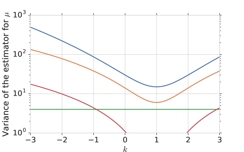
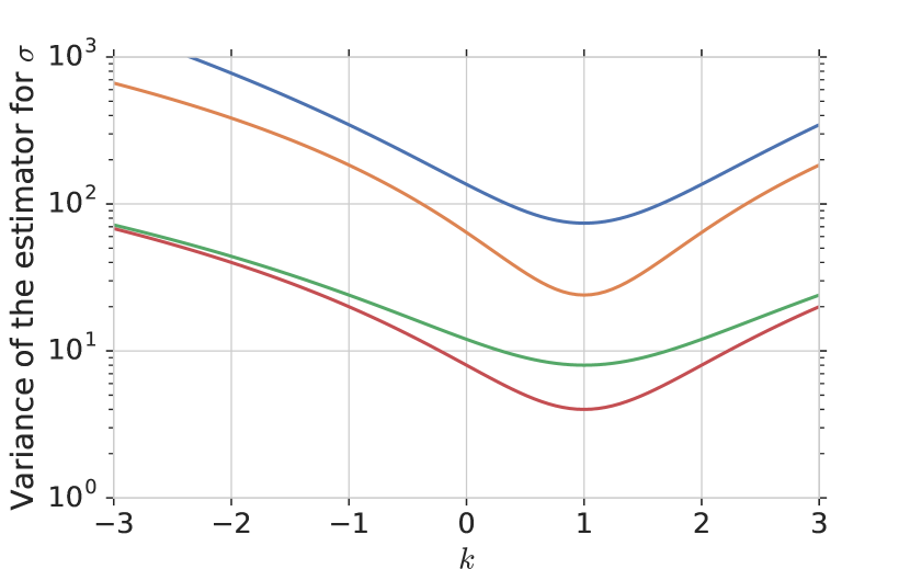
Figure 2 compares the variance of several gradient estimators, for the quadratic function . For this function we see that we could create a rule-of-thumb ranking: the highest variance estimator is the score function, lower variance is obtained by the pathwise derivative, and the lowest variance estimator is the measure-valued derivative. But for the gradient with respect to the mean , we also see that this is not uniformly true, since there are quadratic functions, those with small or large offsets , for which the variance of the pathwise estimator is lower than the measure-valued derivative. This lack of universal ranking is a general property of gradient estimators.
The computational cost of the estimators in Figure 2 is the same for the score-function and pathwise estimators: they can both be computed using a single sample in the Monte Carlo estimator ( in (3)), even for multivariate distributions, making them computationally cheap. The measure-valued derivative estimator will require evaluations of the cost function for dimensional parameters, and for this the reason will typically not be preferred in high-dimensional settings. We will later find that if the cost function is not differentiable, then the pathwise gradient will not be applicable. These are considerations which will have a significant impact on the choice of gradient estimator for any particular problem.








Exponential and Cosine costs.
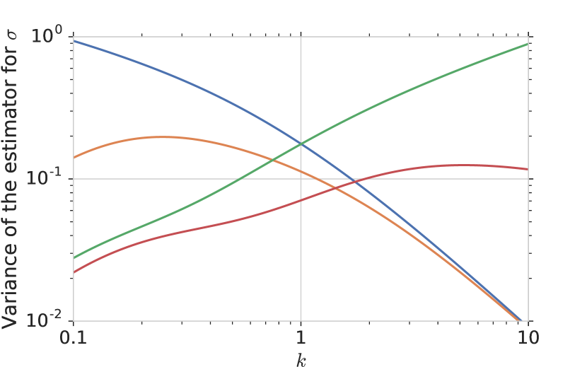
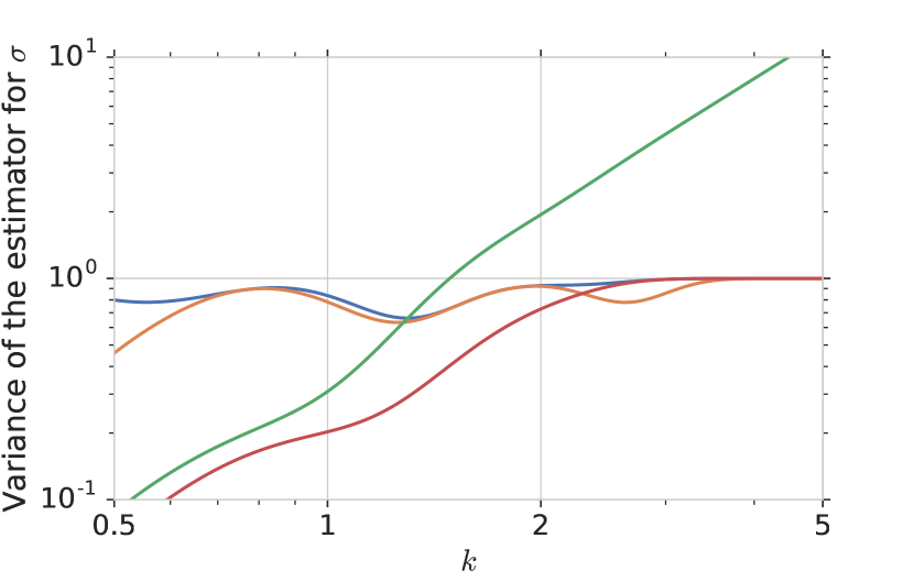
Figure 3 shows the variance behaviour for two other functions, and . As the parameter of these functions varies, the functions can become very sharp and peaked (see the black graphs at the bottom), and this change in the cost function can change the effectiveness of a gradient estimator: from being the lowest-variance estimator in one regime, to being the highest-variance one in another. The green curve in Figure 3 for the pathwise estimator shows its variance increasing as becomes larger. The measure-valued derivative (red curve) has similar behaviour. The blue curve for the score function for the exponential cost shows that its variance can behave in the opposite way, and can be lower for higher values of . We highlight this because, in machine learning applications, we usually learn the cost function (by optimising its structural parameters), and face a setting akin to varying in these graphs. Therefore the process of learning influences the variance behaviour of an estimator differently at different times over the course of learning, which we will need to take steps to control.
Figures 2 and 3 also demonstrate the importance of variance reduction. The score function estimator is commonly used with a control variate, a way to reduce the variance of the gradient that we explore further in Section 7. We see a large decrease in variance by employing this technique. The variance of the measure-valued derivative estimator in these plots is also shown with a form of variance reduction (known as coupling), and for these simple cost functions, there are regimes of the function that allow corrections that drive the variance to zero; we can see this where the kink in the plot for the variance of the mean-gradient for the cosine cost function.
From this initial exploration, we find that there are several criteria to be judged when choosing an unbiased gradient estimator: computational cost, implications on the use of differentiable and non-differentiable cost functions, the change in behaviour as the cost itself changes (e.g., during learning), and the availability of effective variance reduction techniques to achieve low variance. We will revisit these figures again in subsequent sections as we develop the precise description of these methods. We will assess each estimator based on these criteria, working towards building a deeper understanding of them and their implications for theory and practice.
4 Score Function Gradient Estimators
The score function estimator is in the class of derivatives of measure, and is one of the most general types of gradient estimators available to us. Because of its widespread and general-purpose nature, it appears under various names throughout the literature, including the score function estimator (Kleijnen and Rubinstein, 1996; Rubinstein et al., 1996), the likelihood ratio method (Glynn, 1990), and the REINFORCE estimator (Williams, 1992). In this section, we will derive the estimator, expose some of its underlying assumptions and possible generalisations, explore its behaviour in various settings, and briefly review its historical development.
4.1 Score Functions
The score function is the derivative of the log of a probability distribution with respect to its distributional parameters, which can be expanded, using the rule for the derivative of the logarithm, as
| (11) |
This identity is useful since it relates the derivative of a probability to the derivative of a log-probability; for Monte Carlo estimators it will allow us to rewrite integrals of gradients in terms of expectations under the measure . It is the appearance of the score function in the gradient estimator we develop in this section that will explain its name.
The score function is important since, amongst other uses, it is the key quantity in maximum likelihood estimation (Stigler, 2007). One property of the score that will later be useful is that its expectation is zero:
| (12) |
We show this in (12) by first replacing the score using the ratio given by the identity (11), then cancelling terms, interchanging the order of differentiation and integration, and finally recognising that probability distributions must integrate to one, resulting in a derivative of zero. A second important property of the score is that its variance, known as the Fisher information, is an important quantity in establishing the Cramer-Rao lower bound (Lehmann and Casella, 2006).
4.2 Deriving the Estimator
Using knowledge of the score function, we can now derive a general-purpose estimator for the sensitivity analysis problem (2); its derivation is uncomplicated and insightful.
| (13a) | ||||
| (13b) | ||||
| (13c) | ||||
| (13d) | ||||
In the first line (13a), we expanded the definition of the expectation as an integral and then exchanged the order of the integral and the derivative; we discuss the validity of this operation in Section 4.3.1. In (13b), we use the score identity (11) to replace the gradient of the probability by the product of the probability and the gradient of the log-probability. Finally, we obtain an expectation (13c), which is in the form we need—a product of a distribution we can easily sample from and a function we can evaluate—to provide a Monte Carlo estimator of the gradient in (13d).
Equation (13c) is the most basic form in which we can write this gradient. One simple modification replaces the cost function with a shifted version of it
| (14) |
where is a constant that we will call a baseline. For any value of , we still obtain an unbiased estimator because the additional term it introduces has zero expectation due to the property (12) of the score. This baseline-corrected form should be preferred to (13c), because, as we will see in Section 7, it allows for a simple but effective form of variance reduction.
4.3 Estimator Properties and Applicability
By inspecting the form (13c), we can intuitively see that the score-function estimator relates the overall gradient to the gradient of the measure reweighted by the value of the cost function. This intuitiveness is why the score function estimator was one of the first and most widely-used estimators for sensitivity analysis. But there are several properties of the score-function gradient to consider that have a deep impact on its use in practice.
4.3.1 Unbiasedness
When the interchange between differentiation and integration in (13a) is valid, we will obtain an unbiased estimator of the gradient (L’Ecuyer, 1995). Intuitively, since differentiation is a process of limits, the validity of the interchange will relate to the conditions for which it is possible to exchange limits and integrals, in such cases most often relying on the use of the dominated convergence theorem or the Leibniz integral rule (Flanders, 1973; Grimmett and Stirzaker, 2001). The interchange will be valid if the following conditions are satisfied:
-
•
The measure is continuously differentiable in its parameters .
-
•
The product is both integrable and differentiable for all parameters .
-
•
There exists an integrable function such that .
These assumptions usually hold in machine learning applications, since the probability distributions that appear most often in machine learning applications are smooth functions of their parameters. L’Ecuyer (1995) provides an in-depth discussion on the validity of interchanging integration and differentiation, and also develops additional tools to check if they are satisfied.
4.3.2 Absolute Continuity
An important behaviour of the score function estimator is exposed by rewriting it in one other way. Here, we consider a scalar distributional parameter and look at its derivatives using first principles.
| (15a) | ||||
| (15b) | ||||
| (15c) | ||||
| (15d) | ||||
| (15e) | ||||
| (15f) | ||||
In the first line (15a), we again exchange the order of integration and differentiation, which we established is safe in most use-cases. We then expand the derivative in terms of its limit definition in (15b), and swap the order of the limit and the integral in (15c). We introduce an identity term in (15d) to allow us to later rewrite the expression as an expectation with respect to the distribution . Finally, we simplify the expression, separating it in two terms (15e), denoting the importance weight , and rewrite the gradient using the expectation notation (15f). It is this final expression that exposes a hidden requirement of the score function estimator.
The ratio in (15f) is similar to the one that appears in importance sampling (Robert and Casella, 2013). Like importance sampling, the estimator makes an implicit assumption of absolute continuity, where we require for all points where . Not all distributions of interest satisfy this property, and failures of absolute continuity can result in a biased gradient. For example, absolute continuity is violated when the parameter defines the support of the distribution, such as the uniform distribution .
Example (Bounded support). Consider the score-function estimator for a cost and distribution , which is differentiable in when ; the score . This is a popular example also used by Glasserman (2013) and Pflug (1996), amongst others. Comparing the two gradients:
| True gradient: | (16a) | ||||
| Score-function gradient: | (16b) | ||||
In this example, the estimator fails to provide the correct gradient because is not absolutely continuous with respect to at the boundary of the support.
4.3.3 Estimator Variance
From the intuitive analysis in Section 3, where we compared the score function estimator to other gradient estimation techniques (which we explore in the subsequent sections), we see that even in those simple univariate settings the variance of the score-function estimator can vary widely as the cost function varies (blue curves in Figures 2 and 3). Starting from the estimator (13d) and denoting the estimator mean as , we can write the variance of the score function estimator for as
| (17) |
which writes out the definition of the variance. Although this is a scalar expression, it allows us to intuitively see that the parameter dimensionality can play an important role in the estimator’s variance because the score function in (17) has the same dimensionality as the distributional parameters. The alternative form of the gradient we explored in Equation (15f) provides another way to characterise the variance
| (18) |
which, for a fixed , exposes the dependency of the variance on the importance weight . Although we will not explore it further, we find it instructive to connect these variance expressions to the variance bound for the estimator given by the Hammersley-Chapman-Robbins bound (Lehmann and Casella, 2006, ch 2.5)
| (19) |
which is a generalisation of the more widely-known Cramer-Rao bound and describes the minimal variance achievable by the estimator.
Our understanding of the gradient variance can then be built by exploring three sources of variance: contributions from the implicit importance ratio that showed the need for absolute continuity, contributions from the dimensionality of the parameters, and contributions from the variance of the cost function. These are hard to characterise exactly for general cases, but we can develop an intuitive understanding by unpacking specific terms of the gradient variance.
Variance from the importance ratio .
The variance characterisation from either Equation (18) or (19) shows that the importance ratio directly affects the variance. The simplest way to see this effect is to consider the contributions to the variance using the form of the gradient in Equation (15e), for a fixed . The first term in that equation is the quadratic term
| (20) |
where is the importance ratio we identified in Equation (15e). We will obtain finite variance gradients when the integral in (20) is finite, i.e. when the conditions for absolute continuity are satisfied. We saw previously that failures of absolute continuity can lead to biased gradients. In practice, complete failure will be rare and we will instead face near-failures in maintaining absolute continuity, which as the above expression shows, will lead to an increase in the variance of the Monte Carlo estimator of the gradient.
Variance due to input dimensionality.
Assume for simplicity that the distribution factorises over the dimensions of so that , and again consider a scalar parameter . In expectation, the importance weights have the property that for any dimension , The importance weight and its logarithm are given by and , which we can use to study the behaviour of the importance weight as the dimensionality of changes.
If we follow an argument due to Glynn and Iglehart (1989) and Glasserman (2013, p. 259), and assume that the expectation of the log-ratio is bounded, i.e. , then using the strong law of large numbers we can show that this expectation converges to a constant, . Using Jensen’s inequality, we know that , with equality only when , meaning . As a result, the sum of many such terms has a limiting behaviour:
| (21) |
where we reach the limit in the first term since it is a sum of negative terms, and the second expression is obtained by exponentiation. As the dimensionality increases, we find that the importance weights converge to zero, while at the same time their expectation is one for all dimensions. This difference between the instantaneous and average behaviour of means that in high dimensions the importance ratio can become highly skewed, taking large values with small probabilities and leading to high variance as a consequence.
Variance from the cost.
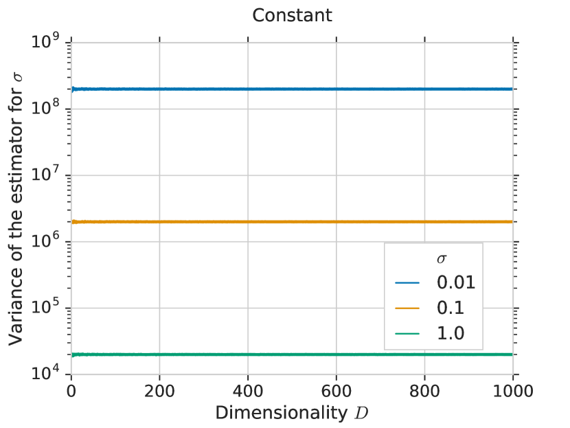
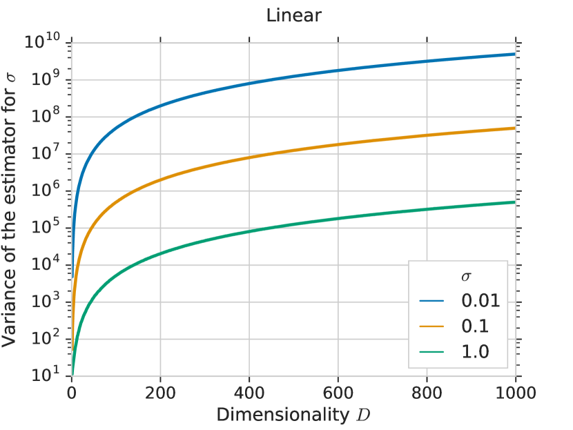
The cost function appears in all forms of the variance we wrote (17)–(19) and is itself a significant contributor to the estimator variance, since it is a multiplicative term in the gradient. For example, if the cost function is a sum of terms, , whose individual variance we assume is bounded, then the variance of the score-function estimator will be of order . Because the cost function is a black-box as far as the estimator is concerned, it will typically contain many elements that do not directly influence the parameters, and hence will not affect the gradient. But every extra term contributes to its variance: ideally, before multiplying the cost with the score function, we would eliminate the parts of it that have no influence on the parameter whose derivative we are computing. Alternatively, we can try to do this automatically by using the gradient of the function itself (but only if it is available) to remove these terms—this approach is explored in the next section.
To support this intuition, we explore the effect of the cost function and measure on the variance properties of the score-function estimator using an example. Figure 4 shows the estimator variance for the gradient , for a constant cost and a linear cost that sums the dimensions of for . For both cost functions, the expected value of the cost under the measure has no dependence on the scale parameter . As we expected, for the linear cost, the variance scales quadratically as the number of terms in the cost increases.
This variance analysis is meant to emphasise the importance of understanding the variance in our estimators. Whether because of the influence of the structure of the cost function, or the dimensionality of the implied importance weights in our gradients, we will need to counterbalance their effects and remove excess variance by some method of variance reduction. The question of variance reduction will apply to every type of Monte Carlo gradient estimator, but the specific solutions that are used will differ due to the different assumptions and properties of the estimator. We will study variance reduction in more detail in Section 7.
4.3.4 Higher-order Gradients
Higher derivatives are conceptually simple to compute using the score function estimator. The score of higher orders is defined as
| (22) |
where represents the th-order gradient operator; unlike the first-order score, higher-order score functions are not defined in terms of higher derivatives of a log-probability. Using this definition, the higher-order score-function gradient estimator is
| (23) |
This simple mathematical shorthand hides the complexity of computing higher-order gradients. Foerster et al. (2018) explore this further, and we expand on this discussion in Section 9 on computational graphs.
4.3.5 Computational Considerations
We can express the score-function gradient estimator (for a single parameter) in one other way, as
| (24) | |||
| (25) |
The first identity shows that the score function gradient can be interpreted as a measure of covariance between the cost function and the score function (and is true because the expectation of the score is zero, which will remove the second term that the covariance would introduce, Pflug (1996) pp. 234). The second identity is the Cauchy-Schwartz inequality, which bounds the squared covariance. Computationally, this shows that the variance of the cost function is related to the magnitude and range of the gradient. A highly-variable cost function can result in highly-variable gradients, which is undesirable for optimisation. It is for this reason that we will often constrain the values of the cost function by normalising or bounding its value in some way, e.g., by clipping.
The score-function gradient is considered to be general-purpose because it is computed using only the final value of the cost in its computation. It makes no assumptions about the internal structure of the cost function, and can therefore be used with any function whose outcome we can simulate; many functions are then open to us for use: known differentiable functions, discrete functions, dynamical systems, or black-box simulators of physical/complex systems or graphics engines. Overall the computational cost of the score function estimator is low; it is of the order for -dimensional distributional parameters , where is the cost of evaluating the cost function, and is the number of samples used in the estimator.
Taking into account the exposition of this section, points for consideration when using the score function estimator are:
-
•
Any type of cost function can be used, allowing for the use of simulators and other black-box systems, as long as we are able to evaluate them easily.
-
•
The measure must be differentiable with respect to its parameters, an assumption we make throughout this paper.
-
•
We must be able to easily sample from the measure, since the gradient estimator is computed using samples from it.
-
•
It is applicable to both discrete and continuous distributions, which adds to its generality.
-
•
The estimator can be implemented using only a single sample if needed, i.e. using . Single-sample estimation is applicable in both univariate and multivariate cases, making the estimator computationally efficient, since we can deliberately control the number of times that the cost function is evaluated.
-
•
Because there are many factors that affect the variance of the gradient estimator, it will be important to use some form of variance reduction to obtain competitive performance.
4.4 Research in Score Function Gradient Estimation
We are the lucky inheritors of a rich body of work specifically devoted to the score function gradient estimator. Given its simplicity and generality, this estimator has found its way to many parts of computational science, especially within operations research, computational finance, and machine learning. We describe a subset of this existing work, focusing on the papers that provide deeper theoretical insight and further context on the score-function estimator’s use in practice.
Development of the estimator.
The score function estimator is one of the first types of estimators to be derived, initially by several different groups in the 1960s, including Miller (1967) in the design of stable nuclear reactors, and Rubinstein (1969) in the early development of Monte Carlo optimisation. Later the estimator was derived and applied by Rubinstein and Kreimer (1983) for discrete-event systems in operations research, where they began to refer to the estimator as the score function method, the name we use in this paper. The estimator was again developed by Glynn (1987, 1990) and by Reiman and Weiss (1989), where they referred to it as the likelihood ratio method, and part of the study of queueing systems and regenerative stochastic processes. Concise descriptions are available in several books, such as those by Rubinstein and Shapiro (1993) and Fu and Hu (2012), as well as in two books we especially recommend by Pflug (1996, sect. 4.2.1) and Glasserman (2013, sect 7.3).
Interchange of integration and differentiation.
The two basic questions for the application of the score-function estimator are differentiability of the stochastic system that is being studied, and subsequently, the validity of the interchange of integration and differentiation. For many simple systems, differentiability can be safely assumed, but in discrete-event systems that are often studied in operations research, some effort is needed to establish differentiability, e.g., like that of the stochastic recursions by Glynn and L’Ecuyer (1995). The validity of the interchange of differentiation and integration for score function estimators is discussed by Kleijnen and Rubinstein (1996) and specifically in the note by L’Ecuyer (1995).
In machine learning.
In reinforcement learning, the score-function gradient estimator was developed as the REINFORCE algorithm by Williams (1992). In such settings, the gradient is the fundamental quantity needed for policy search methods and is the basis of the policy gradient theorem and the subsequent development of actor-critic reinforcement learning methods (Sutton et al., 2000). Approximate Bayesian inference methods based on variational inference deployed the score function gradient estimator to enable a more general-purpose, black-box variational inference; one that did not require tedious manual derivations, but that could instead be more easily combined with automatic differentiation tools. The appeal and success of this approach has been shown by several authors, including Paisley et al. (2012), Wingate and Weber (2013), Ranganath et al. (2014), and Mnih and Gregor (2014). Variance reduction is essential for effective use of this estimator, and has been explored in several areas, by Greensmith et al. (2004) in reinforcement learning, Titsias and Lázaro-Gredilla (2015) in variational inference, Capriotti (2008) in computational finance, and more recently by Walder et al. (2019). We describe variance reduction techniques in more detail in Section 7. Finally, as machine learning has sought to automate the computation of these gradients, the implementation of the score function estimator within wider stochastic computational graphs has been explored for the standard estimator (Schulman et al., 2015) and its higher-order counterparts (Foerster et al., 2018); we will provide more discussion on computational graphs in Section 9.
5 Pathwise Gradient Estimators
We can develop a very different type of gradient estimator if, instead of relying on the knowledge of the score function, we take advantage of the structural characteristics of the problem (2). One such structural property is the specific sequence of transformations and operations that are applied to the sources of randomness as they pass through the measure and into the cost function, to affect the overall objective. Using this sampling path will lead us to a second estimator, the pathwise gradient estimator, which as its name implies, is in the class of derivatives of paths. Because we need information about the path underlying a probabilistic objective, this class of gradient estimator will be less general-purpose than the score-function estimator, but in losing this generality, we will gain several advantages, especially in terms of lower variance and ease of implementation.
The pathwise derivative is as fundamental to sensitivity analysis and stochastic optimisation as the score function estimator is, and hence also appears under several names, including: the process derivative (Pflug, 1996), as the general area of perturbation analysis and specifically infinitesimal perturbation analysis (Ho and Cao, 2012; Glasserman and Ho, 1991), the pathwise derivative (Glasserman, 2013), and more recently as the reparameterisation trick and stochastic backpropagation (Rezende et al., 2014; Kingma and Welling, 2014b; Titsias and Lázaro-Gredilla, 2014). Another way to view the pathwise approach is as a process of pushing the parameters of interest, which are part of the measure, into the cost function, and then differentiating the newly-modified cost function. For this reason, the pathwise estimator is also called the ‘push-in’ gradient method (Rubinstein, 1992).
5.1 Sampling Paths
Continuous distributions have a simulation property that allows both a direct and an indirect way of drawing samples from them, making the following sampling processes equivalent:
| (26) |
and states that an alternative way to generate samples from the distribution is to sample first from a simpler base distribution , which is independent of the parameters , and to then transform this variate through a deterministic path ; we can refer to this procedure as either a sampling path or sampling process. For invertible paths, this transformation is described by the rule for the change of variables for probability
| (27) |
There are several classes of transformation methods available (Devroye, 2006):
-
•
Inversion methods. For univariate distributions, we will always be able to find an equivalent base distribution and sampling path by using the uniform distribution and inverse cumulative distribution function (CDF), respectively. This method can often be difficult to use directly, however, since computing the inverse of the CDF and its derivative can be computationally difficult, restricting this approach to univariate settings. We will return to this method later, but instead explore methods that allow us to use the CDF instead of its inverse.
-
•
Polar transformations. It is sometimes possible, and more efficient, to generate a pair of random variates from the target distribution . We can map this pair to a representation in polar form , which exposes other mechanisms for sampling, e.g., the famous Box-Muller transform for sampling Gaussian variates is derived in this way.
-
•
One-liners. In many cases there are simple functions that transform a base distribution into a richer form. One widely-known example is sampling from the multivariate Gaussian , by first sampling from the standard Gaussian , and then applying the location-scale transformation , with . Many such transformations exist for common distributions, including the Dirichlet, Gamma, and Exponential. Devroye (1996) refers to these types of transformations as one-liners because they can often be implemented in one line of code.
With knowledge of these transformation methods, we can invoke the Law of the Unconscious Statistician (LOTUS) (Grimmett and Stirzaker, 2001)
| (28) |
which states that we can compute the expectation of a function of a random variable without knowing its distribution, if we know its corresponding sampling path and base distribution. LOTUS tells us that in probabilistic objectives, we can replace expectations over any random variables wherever they appear, by the transformation and expectations over the base distribution . This is a way to reparameterise a probabilistic system; it is often used in Monte Carlo methods, where it is referred to as the non-centred parameterisation (Papaspiliopoulos et al., 2007) or as the reparameterisation trick (Kingma and Welling, 2014b).
5.2 Deriving the Estimator
Equipped with the pathwise simulation property of continuous distributions and LOTUS, we can derive an alternative estimator for the sensitivity analysis problem (2) that exploits this additional knowledge of continuous distributions. Assume that we have a distribution with known differentiable sampling path and base distribution . The sensitivity analysis problem (2) can then be reformulated as
| (29a) | ||||
| (29b) | ||||
| (29c) | ||||
| (29d) | ||||
In Equation (29a) we first expand the definition of the expectation. Then, using the law of the unconscious statistician, and knowledge of the sampling path and the base distribution for , we reparameterise this integral (29b) as one over the variable . The parameters have now been pushed into the function making the expectation free of the parameters. This allows us to, without concern, interchange the derivative and the integral (29c), resulting in the pathwise gradient estimator (29d).
5.3 Estimator Properties and Applicability
The gradient (29c) shows that we can compute gradients of expectations by first pushing the parameters into the cost function and then using standard differentiation, applying the chain rule. This is a natural way to think about these gradients, since it aligns with our usual understanding of how deterministic gradients are computed, and is the reason this approach is so popular. Since the sampling path need not always be invertible, the applicability of the estimator goes beyond the change of variable formula for probabilities (27). Its simplicity, however, belies several distinct properties that impact its use in practice.
5.3.1 Decoupling Sampling and Gradient Computation
The pathwise estimator (29c), as we derived it, is limited to those distributions for which we simultaneously have a differentiable path, and use this same path to generate samples. We could not compute gradients with respect to parameters of a Gamma distribution in this way, because sampling from a Gamma distribution involves rejection sampling which does not provide a differentiable path. The process of sampling from a distribution and the process of computing gradients with respect to its parameters are coupled in the estimator (29c); we can expand the applicability of the pathwise gradient by decoupling these two processes.
The pathwise estimator can be rewritten in a more general form:
| (30a) | ||||
| (30b) | ||||
In the first line (30a), we recall the gradient that was formed as a result of applying the law of the unconscious statistician in Equation (29c), and then apply the chain rule to write the gradient w.r.t. . Using the LOTUS (28) again, this time for the expectation of and in the reverse direction, we obtain (30b). This derivation shows that sampling and gradient estimation can be decoupled: we can generate samples using any sampler for the original distribution (e.g., using a sampling path, rejection sampling, or Markov chain Monte Carlo), and compute the gradient using the chain rule on the function by finding some way to compute the term .
One way to compute is to use as we did for (29c). In practice, this form is not always convenient. For example, if the sampling path is an inverse cumulative density function (inverse CDF), which is often computed with root-finding methods, then evaluating its derivative may require numerically unstable finite difference methods. Instead, we can find another way of writing that makes use of the inverse of the path . We can think of as the ‘standardisation path’ of the random variable—that is the transformation that removes the dependence of the sample on the distribution parameters, standardising it to a zero mean unit variance-like form. In the univariate case, instead of using the inverse CDF, we can use the standardisation path given by the CDF. Consider the equation as an implicit function for . Evaluating the total derivative (TD) on both sides—using implicit differentiation—and expanding we find that
| (31a) | |||
| (31b) | |||
| (31c) | |||
Equation (31c) gives us the expression needed to fully evaluate (30b). Equation (31c) is the form in which Ho and Cao (1983) initially introduced the estimator, and it corresponds to the strategy of differentiating both sides of the transformation noted by Glasserman (2013). Figurnov et al. (2018) refer to this approach to as an implicit reparameterisation gradient, because of its use of implicit differentiation. In this form, we are now able to apply pathwise gradient estimation to a far wider set of distributions and paths, such as for the Beta, Gamma, and Dirichlet distributions. In Section 8 we look at this decoupling in other settings, and in the discussion (Section 9.4) look at optimal transport as another way of computing .
Example (Univariate Gaussian). For univariate Gaussian distributions , with , the location-scale transform is the natural choice of the path: for . The inverse path is then . The standard pathwise derivatives are and . Equation (31c) is then
| (32) |
We see that the two approaches provide the same gradient.
Example (Univariate distributions). As we discussed, for univariate distributions we can use the sampling path given by the inverse CDF: , where . Computing the derivative is often complicated and expensive. We can obtain an alternative expression for by considering the inverse path, which is given by the CDF . From Equation (31c) we have
| (33) |
In the final step, we used the fact that the derivative of the CDF w.r.t. is the density function. This expression allows efficient computation of pathwise gradients for a wide range of continuous univariate distributions, including Gamma, Beta, von Mises, Student’s , as well as univariate mixtures (Figurnov et al., 2018; Jankowiak and Obermeyer, 2018).
5.3.2 Bias and Variance Properties
In deriving the pathwise estimator (29d) we again exploited an interchange of differentiation and integration. If this interchange is valid, then the resulting application of the chain rule to compute the gradient will be valid as well, and the resulting estimator will be unbiased. We can always ensure that this interchange applies by ensuring that the cost functions we use are differentiable. The implication of this is that we will be unable to use the pathwise gradient estimator for discontinuous cost functions. We can be more rigorous about the conditions for unbiasedness, and we defer to Glasserman (2013, sect. 7.2.2) for this more in-depth discussion.
The variance of the pathwise estimator can be shown to be bounded by the squared Lipschitz constant of the cost function (Glasserman, 2013, sect. 7.2.2). This result is also shown by Fan et al. (2015, sect. 10) for the case of gradients (2) with Gaussian measures, instead using the properties of sub-Gaussian random variables, deriving a dimension-free bound for the variance in terms of the squared Lipschitz constant. This insight has two important implications for the use of the pathwise gradient. Firstly, the variance bounds that exist are independent of the dimensionality of the parameter space, meaning that we can expect to get low-variance gradient estimates, even in high-dimensional settings. Because we are able to differentiate through the cost function itself, only the specific path through which any individual parameter influences the cost function is included in the gradient (automatic provenance tracking); unlike the score-function estimator, the gradient does not sum over terms for which the parameter has no effect, allowing the estimator variance to be much lower. Secondly, as Figures 2 and 3 show, as the cost function becomes highly-variable, i.e. its Lipschitz constant increases, we enter regimes where, even with the elementary functions we considered, the variance of the pathwise estimator can be higher than that of the score-function method. The pathwise gradient, when it is applicable, will not always have lower variance when compared to other methods since its variance is directly bounded by the cost function’s Lipschitz constant. In such situations, variance reduction will again be a powerful accompaniment to the pathwise estimator. Since most of the functions we will work with will not be Lipschitz continuous, Xu et al. (2018) use a different set of simplifying assumptions to develop an understanding of the variance of the pathwise estimator that reinforces the general intuition built here.
5.3.3 Higher-order Gradients
Computation of higher-order gradients using the pathwise method is also possible and directly involves higher-order differentiation of the function, requiring cost functions that are differentiable at higher-orders. This approach has been explored by Fu and Hu (1993) and Fan et al. (2015). Another common strategy for computing higher-order gradients is to compute the first-order gradient using the pathwise methods, and the higher-order gradients using the score-function method.
5.3.4 Computational Considerations
The pathwise gradient estimator is restricted to differentiable cost functions. While this is a large class of functions, this limitation makes the pathwise estimator less broadly applicable than the score-function estimator. For some types of discontinuous functions it is possible to smooth the function over the discontinuity and maintain the correctness of the gradient; this approach is often referred to as smoothed perturbation analysis in the existing literature (Glasserman and Ho, 1991).
Often there are several competing approaches for computing the gradient. The choice between them will need to be made considering the associated computational costs and ease of implementation. The case of the univariate Gaussian measure highlights this. This distribution has two equivalent sampling paths: one given by the location-scale transform: and another given by the inverse CDF transform: . While there is no theoretical difference between the two paths, the first path is preferred in practice due to the simplicity of implementation.
The same analysis we pointed to relating to the variance of the Gaussian gradient earlier, also provides a tail bound with which to understand the convergence of the Monte Carlo estimator (Fan et al., 2015). Rapid convergence can be obtained even when using only a single sample to compute the gradient, as is often done in practice. There is a trade-off between the number of samples used and the Lipschitz constant of the cost function, and may require more samples to be used for functions with higher Lipschitz constants. This consideration is why we will find that regularisation that promotes smoothness of the functions we learn is important for successful applications. Overall, the computational cost of the pathwise estimator is the same as the score function estimator and is low, of the order , where is the dimensionality of the distributional parameters , is the cost of evaluating the cost function and its gradient, and is the number of samples used in the estimator.
Taking into account the exposition of this section, points for consideration when using the pathwise derivative estimator are:
-
•
Only cost functions that are differentiable can be used.
-
•
When using the pathwise estimator (29c), we do not need to know the measure explicitly. Instead we must know its corresponding deterministic and differentiable sampling path and a base distribution that is easy to sample from.
-
•
If using the implicit form of the estimator, we require a method of sampling from the original distribution as well as a way of computing the derivative of the inverse (standardisation) path.
-
•
The estimator can be implemented using only a single sample if needed, i.e. using . Single-sample estimation is applicable in both univariate and multivariate cases, making the estimator computationally efficient, since we can deliberately control the number of times that the cost function is evaluated.
-
•
We might need to control the smoothness of the function during learning to avoid large variance, and may need to employ variance reduction.
5.4 Research in Pathwise Derivative Estimation
Basic development.
This pathwise estimator was initially developed by Ho and Cao (1983) under the name of infinitesimal perturbation analysis (IPA), by which it is still commonly known. Its convergence properties were analysed by Heidelberger et al. (1988). Other variations of perturbation analysis expand its applicability, see Suri and Zazanis (1988) and the books by Glasserman and Ho (1991) and Ho and Cao (2012). The view as a push-in technique was expanded on by Rubinstein (1992). Again, the books by Glasserman (2013, sect. 7.2) and Pflug (1996, sect. 4.2.3) provide a patient exploration of this method using the names of the pathwise derivative and process derivative estimation, respectively.
Appearance in machine learning.
The pathwise approach to gradient estimation has seen wide application in machine learning, driven by work in variational inference. An early instance of gradients of Gaussian expectations in machine learning was developed by Opper and Archambeau (2009). Rezende et al. (2014) called their use of the pathwise estimator stochastic backpropagation, since the gradient reduced to the standard gradient computation by backpropagation averaged over an independent source of noise. As we mentioned in Section 2.2, Titsias and Lázaro-Gredilla (2014) used the pathwise estimator under the umbrella of doubly stochastic optimisation, to recognise that there are two distinct sources of stochasticity that enter when using the pathwise estimator with mini-batch optimisation. The substitution of the random variable by the path in the estimator (29d) led Kingma and Welling (2014a, b) to refer to their use of the substitution as the reparameterisation trick, and by which it is commonly referred to at present in machine learning.
Use in generative models and reinforcement learning.
Recognising that the pathwise gradients do not require knowledge of the final density, but only a sampling path and base distribution, Rezende and Mohamed (2015) developed normalising flows for variational inference, which allows learning of complex probability distributions that exploit this property of the pathwise estimator. Since the pathwise estimator does not require invertible sampling paths, it is very suited for uses with very expressive but not invertible function approximators, such as deep neural networks. This has been used to optimise model parameters in implicit generative models, such those in generative adversarial networks (Goodfellow et al., 2014; Mohamed and Lakshminarayanan, 2016). To learn behaviour policies in continuous action spaces, the pathwise estimator has also found numerous uses in reinforcement learning for continuous control. Williams (1992, sect. 7.2) invoked this approach as an alternative to the score function when using Gaussian distributions, and has also been used for learning value gradients by Heess et al. (2015) and Lillicrap et al. (2016). We find that the pathwise derivative is now a key tool for computing information-theoretic quantities like the mutual information (Alemi et al., 2017), in Bayesian optimisation (Wilson et al., 2018) and in probabilistic programming (Ritchie et al., 2016).
Derivative generalisations.
Gong and Ho (1987) introduced smoothed perturbation analysis as one variant of the pathwise derivative to address cases where the interchange of differentiation and integration is not applicable, such as when there are discontinuities in the cost function; and several other extensions of the estimator appear in the perturbation analysis literature (Glasserman and Ho, 1991). In the variational inference setting, Lee et al. (2018) also look at the non-differentiable case by splitting regions into differentiable and non-differentiable components. The implicit reparameterisation gradients for univariate distributions were developed by Salimans and Knowles (2013). Hoffman and Blei (2015) used the implicit gradients to perform backpropagation through the Gamma distribution using a finite difference approximation of the CDF derivative. Graves (2016) derived the implicit reparameterisation gradients for multivariate distributions with analytically tractable CDFs, such as mixtures. The form of implicit reparameterisation that we described here was developed by Figurnov et al. (2018) and clarifies the connections to existing work and provides further practical insight. Other generalisations like that of Ruiz et al. (2016), Naesseth et al. (2017), and Parmas et al. (2018), combine the score function method with the pathwise methods; we come back to these hybrid methods in Section 8.
6 Measure-valued Gradients
A third class of gradient estimators, which falls within the class of derivatives of measure, is known simply as the measure-valued gradient estimators, and has received little attention in machine learning. By exploiting the underlying measure-theoretic properties of the probabilities in the sensitivity analysis problem (2)—the properties of signed-measures in particular—we will obtain a class of unbiased and general-purpose gradient estimators with favourable variance properties. This approach is referred to interchangeably as either the weak derivative method (Pflug, 1996) or as the measure-valued derivative (Heidergott and Vázquez-Abad, 2000).
6.1 Weak Derivatives
Consider the derivative of a density with respect to a single parameter , with the index on the set of distributional parameters. The derivative is itself not a density, since it may have negative values and does not integrate to one. However, using the properties of signed measures, we can always decompose this derivative into a difference of two densities, each multiplied by a constant (Pflug, 1989):
| (34) |
where are densities, referred to as the positive and negative components of , respectively. By integrating both sides of (34), we can see that :
Therefore, we can simply use one constant that we denote , and the decomposition becomes
| (35) |
The triple is referred to as the (th) weak derivative of . We restrict our definition here to the univariate parameter case; the multivariate parameter case extends this definition to form a vector of triples, with one triple for each dimension. We list the weak derivatives for several widely-used distributions in Table 1, and defer to Heidergott et al. (2003) for their derivations.
| Distribution | Constant | Positive part | Negative part |
|---|---|---|---|
| Bernoulli() | 1 | ||
| Poisson() | 1 | ||
| Normal() | |||
| Normal() | |||
| Exponential() | |||
| Gamma() | |||
| Weibull() |
The derivative is weak because we do not require the density to be differentiable on its domain, but rather require that integrals of the decomposition against sets of test functions converge. For example, the decomposition of mass functions of discrete distributions results in positive and negative components that are delta functions, which are integrable against continuous functions. The weak derivative is not unique, but always exists and can be obtained using the Hahn-Jordan decomposition of a signed measure into two measures that have complementary support (Billingsley, 2008). Like the score function and the sampling path, the weak derivative is a tool we will use to study the sensitivity analysis problem (2), although it has uses in other settings. The connections between the weak derivative and functional analysis, as well as a general calculus for weak differentiability is described by Heidergott and Leahu (2010).
6.2 Deriving the Estimator
Using our knowledge of weak derivatives of probability measures, we can now derive a third estimator for the gradient problem (2). This will lead us to an unbiased gradient estimator, which intuitively computes the gradient using a weighted difference of two expectations. For -dimensional parameters , we can rewrite the gradient for the th parameter as
| (36a) | ||||
| (36b) | ||||
| (36c) | ||||
| (36d) | ||||
In the first line (36a) we expanded the expectation as an integral and then interchanged the order of differentiation and integration. In the second line (36b), we substituted the density-derivative with its weak derivative representation (35). We use the symbols to remind ourselves that the positive and negative components may be different depending on which parameter of the measure the derivative is taken with respect to, and to indicate that the constant will also change depending on the parameter being differentiated. We write the gradient using the expectation operators we have used throughout the paper (36c), and finally obtain an estimator in Equation (36d).
The triple is the measure-valued gradient of (2) (Pflug, 1989; Heidergott et al., 2003). We now have a third unbiased estimator of the gradient that applies to any type of cost functions , differentiable or not, since no knowledge of the function is used other than our ability to evaluate it for different inputs.
Example (Bernoulli measure-valued gradient). We can illustrate the generality of the measure-valued derivatives by considering the case where is the Bernoulli distribution.
| (37) |
The weak derivative is given by the triple , where denotes the Dirac measure at . This example is also interesting, since in this case, the measure-valued estimator is the same as the estimator that would be derived using the score-function approach.
Example (Gaussian measure-valued gradient). We now derive the measure-valued derivative for the probabilistic objective (1) w.r.t. the mean parameter of a Gaussian measure; we will do this from first principles, rather than relying on the result in Table 1. We will make use of the change of variables , with differentials in this derivation.
| (38a) | ||||
| (38b) | ||||
| (38c) | ||||
| (38d) | ||||
| (38e) | ||||
| (38f) | ||||
In the first line we exchange the order of integration and differentiation, and in the second line (38b) differentiate the Gaussian density with respect to its mean . The derivative is written in a form that decomposes the integral around the mean , and in this way introduces the minus sign needed for the form of the weak derivative. In the third line, we split the integral over the domains implied by the decomposition. The fourth line changes the limits of the second integral to the domain of , which is used in the next line (38e) along with the change of variables to rewrite the integral more compactly in terms of . In the final line (38f) we recognise the Weibull distribution with zero-shift as the new measure under which the integral is evaluated and write the expression using the expectation notation we use throughout the paper. We give the form of the Weibull and other distributions in Appendix A.
Equation (38f) gives the measure-valued derivative as the difference of two expectations under the Weibull distribution weighted by a constant, and can be described by the triple and estimator
| (39) |
In Equation (39) the samples used for positive and negative parts are independent. A simple variance reduction is possible by coupling the two Weibull distributions with a set of common random numbers; we explore variance reduction by coupling in more detail later.
While we have restricted ourselves to scalar quantities in these derivations, the same properties extend to the vector case, where the measure-valued derivative is a vector of triples; as Pflug (1996) says, ‘the vector case is more complicated in notation, but not in concept’. In Equation (36a), if the measure is a factorised distribution then the positive and negative components of the weak derivative will itself factorise across dimensions. For the positive component, this decomposition will be , which is the product of the original density for all dimensions except the th dimension, and the positive density decomposition; the same holds for the negative component. For the derivative with respect to the mean when the measure is a diagonal Gaussian in (38a), this decomposition is the product of a Weibull distribution for the th component, and a Gaussian distribution for all other dimensions, which are easy to sample from when forming the estimator. Full-covariance Gaussian measures will follow a similar decomposition, sampling from the multivariate Gaussian and replacing the th component with a Weibull variate.
6.3 Estimator Properties and Applicability
6.3.1 Domination
The two derivatives-of-measure—the score function and the measure-valued derivative—differ in the ways that they establish the correctness of the interchange of differentiation and integration. For the score function estimator, we achieved this in Section 4.3 by invoking the dominated convergence theorem and assuming the gradient estimator is dominated (bounded) by a constant. We explored one example where we were unable to ensure domination (using the example of bounded support in Section 4.3), because no bounding constant applies at the boundaries of the domain. For the weak derivative, the correctness of the interchange of differentiation and integration is guaranteed by its definition: the fundamental property of weak derivatives states that if the triple is a weak derivative of the probability measure , then for every bounded continuous function (Pflug, 1996; Heidergott and Vázquez-Abad, 2000)
| (40) |
We should therefore expect the pathology in the example on bounded support not to appear.
Example (Bounded support revisited). We revisit our earlier example from Section 4.3.2 in which we compute the gradient of the objective (2) using the cost function and distribution , which is differentiable in when . The measure-valued derivative is
| (41a) | ||||
| (41b) | ||||
In the first line, we fixed the limits of integration using the support of the uniform distribution and then applied the product rule for differentiation to obtain the two terms. In the second line (41b), we rewrite the terms to reflect the triple form with which we have been communicating the weak derivative. The measure-valued derivative is given by the triple ; the positive part is a discrete measure whereas the negative part is continuous in the range . Using this result for our specific gradient problem, we find:
| True gradient: | (42a) | ||||
| Measure-valued gradient: | (42b) | ||||
By not requiring domination, the measure-valued derivative achieves the correct value.
6.3.2 Bias and Variance Properties
By using the fundamental property of weak derivatives, which requires bounded and continuous cost functions , we can show that the measure-valued gradient (38f) provides an unbiased estimator of the gradient. Unbiasedness can also be shown for other types of cost functions, such as those that are unbounded, or those with sets of discontinuities that have measure zero under the positive and negative components (Pflug, 1996, sect 4.2).
The variance of the measure-valued derivative estimator is
| (43) |
From this, we see that the variance of the gradient estimator depends on the choice of decomposition of the weak derivative into its positive and negative components. An orthogonal decomposition using the Hahn-Jordan decomposition is suggested to give low variance in general (Pflug, 1989). Furthermore, we see that if the random variables can be ‘coupled’ in some way, where they share the same underlying source of randomness, this can reduce gradient variance by increasing the covariance term in (43). The most common coupling scheme is to sample the variables and using common random numbers—this is what we used in Figures 2 and 3. From the figures, we see that the measure-valued derivative estimator with coupling often provides lower variance than the alternative estimators. Pflug (1996, example 4.21) discusses variance reduction for measure-valued derivatives and approaches for coupling in detail, and we expand on this in Section 7.2.
To examine the effect of the number of measure parameters, data dimensionality, and cost function on the variance of the coupled measure valued gradient estimator, Figure 5 shows the estimator variance for the gradient , for a linear cost for as well as the forth-order cost . We observe that the measure valued estimator is not sensitive to the dimensionality of the measure parameters, unlike the score function estimator (see Figure 4). It is however sensitive to the magnitude of the function, and the variance of the measure, which is reflected in the higher variance for the positive and negative components.
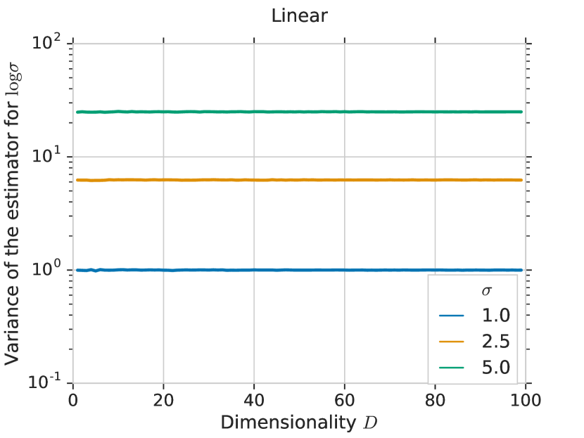
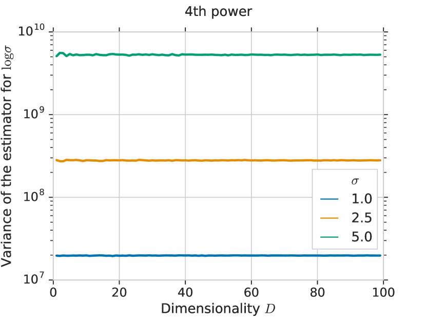
6.3.3 Higher-order Derivatives
The problem of computing higher-order derivatives involves computing . The second derivative is also a signed measure, which means that it too has a weak derivative representation. For higher-order derivatives we will again be able to compute the gradient using a weighted difference of expectations, using the weak-derivative triple , where and are the positive and negative components of the decomposition for the th order density-derivative .
6.3.4 Computational Considerations
Measure-valued gradients are much more computationally expensive than the score-function or pathwise gradients. This is because the gradient we computed in (36d) is the gradient for a single parameter: for every parameter we require two evaluations of the cost function to compute its gradient. It is this structure of adapting the underlying sampling distributions for each parameter that leads to the low variance of the estimator but at the same time makes its application to high-dimensional parameter spaces prohibitive. For problems that do not have a large number of parameters, and for which we can evaluate the cost frequently, e.g., being in the form of a simulator rather than a costly interactive system, this gradient may prove beneficial. Overall the computational cost is , for samples drawn from each of the positive and negative components of the weak derivative, -dimensional parameters , and a cost of evaluating the cost function.
Taking into account the exposition of this section, points for consideration when using the measure-valued derivatives are:
-
•
The measure-valued derivative can be used with any type of cost function, differentiable or not, as long as we can evaluate it repeatedly for different inputs.
-
•
It is applicable to both discrete and continuous distributions, which adds to its generality.
-
•
The estimator is computationally expensive in high-dimensional parameter spaces since it requires two cost function evaluations for every parameter.
-
•
We will need methods to sample from the positive and negative measures, e.g., the double-sided Maxwell distribution for the gradient of the Gaussian variance.
-
•
Using the weak derivative requires manual derivation of the decomposition at first, although for many common distributions the weak-derivative decompositions are known.
6.4 Research in Measure-valued Derivatives
The weak derivative was initially introduced by Pflug (1989), with much subsequent work to establish its key properties, including behaviour under convex combinations, convolution, transformation, restriction, and the use of differentiability of the gradient problem as a sufficient condition for unbiasedness. In most papers, the details of how to derive the weak derivative were omitted; this important exposition was provided for many common distributions by Heidergott et al. (2003). The connections between perturbation analysis (pathwise estimation) and measure-valued differentiation are explored by Heidergott et al. (2003), with specific exploration of Markov processes and queuing theory applications. Heidergott et al. (2008) also provide a detailed exposition for derivatives with Gaussian measures, which is one of the most commonly encountered cases. In machine learning, Buesing et al. (2016) discuss the connection between weak derivatives, finite differences, and other Monte Carlo gradient estimation methods, and Rosca et al. (2019) provide an empirical comparison for problems in approximate Bayesian inference.
7 Variance Reduction Techniques
From the outset, we listed low variance as one of the crucial properties of Monte Carlo estimators. The three classes of gradient estimators we explored each have different underlying conditions and properties that lead to their specific variance properties. But in all cases the estimator variance is something we should control, and ideally reduce, since it will be one of the principal sources of performance issues. As we search for the lowest variance gradient estimators, it is important to recognise a key tension that will develop, between a demand for computationally-efficient and effective variance reduction versus low-effort, generic, or black-box variance reduction tools. We focus on four common methods in this section—large-samples, coupling, conditioning, and control variates. These methods will be described separately, but they can also be combined and used in concert to further reduce the variance of an estimator. Variance reduction is one of the largest areas of study in Monte Carlo methods, with important expositions on this topic provided by Robert and Casella (2013, ch. 4), Owen (2013, ch. 8-10) and Glasserman (2013, ch. 4).
7.1 Using More Samples
The simplest and easiest way to reduce the variance of a Monte Carlo estimator is to increase the number of samples used to compute the estimator (3). The variance of such estimators shrinks as , since the samples are independent, while the computational cost grows linearly in . For a more complex variance reduction method to be appealing, it should compare favourably to this reference method in terms of efficiency of variance reduction. If evaluating the cost function involves only a computational system or simulator, then using more samples can be appealing, since the computational cost can be substantially reduced by parallelising the computation. For some problems, however, increasing the number of Monte Carlo samples will not be an option, typically in problems where evaluating the cost function involves a real-world experiment or interaction. We restricted our discussion to the standard Monte Carlo method, which evaluates the average (3) using independent sets of random variates, but other approaches can provide opportunities for improved estimation. Quasi Monte Carlo methods generate a set of samples that form a minimum discrepancy sequence, which are both more efficient in the use of the samples and can lead to reduced variance, with more to explore in this area (Glasserman (2013, chp. 5), Leobacher and Pillichshammer (2014), Buchholz et al. (2018)).
7.2 Coupling and Common Random Numbers
We will often encounter problems that take the form of a difference between two expectations of a function under different but closely-related distributions and :
| (44) |
We saw this type of estimation problem in the derivation of the measure-valued gradient estimator (36d). The direct approach to computing the difference would be to estimate each expectation separately using independent samples and to then take their difference:
| (45) |
where and are i.i.d. samples from and , respectively. We can achieve a simple form of variance reduction by coupling and in Equation (45), so that each pair is sampled from some joint distribution with marginals and . The variance of the resulting coupled estimator for is
| (46) |
Therefore, to reduce variance we need to choose a coupling such that and are positively correlated. In general, finding an optimal coupling can be difficult, even in the univariate case since it involves the inverse CDFs of and (see e.g. Pflug (1996, p. 225)). The use of common random numbers is one simple and popular coupling technique that can be used when and are close or in a related family of distributions. Common random numbers involve sharing, in some way, the underlying random numbers used in generating the random variates and . For example, in the univariate case, we can do this by sampling and applying the inverse CDF transformations: and .
Example (Maxwell-Gaussian Coupling). Consider Gaussian measures in the setting of Equation (2) and the task of computing the gradient with respect to the standard deviation . The measure-valued gradient, using Table 1, is given by the triple , where is the double-sided Maxwell distribution with location and scale , and is the Gaussian distribution with mean and variance ; see Appendix A for the densities for these distributions. We can couple the Gaussian and the Maxwell distribution by exploiting their corresponding sampling paths with a common random number: if we can generate samples then, by first sampling from the Uniform distribution and reusing the Maxwell samples, we can generate distributed samples via . Then, we can perform a location-scale transform to obtain the desired Maxwell and Normal samples: . The distributions are coupled because they use the same underlying Maxwell-distributed variates (Heidergott et al., 2008). The variance reduction effect of Maxwell-Gaussian coupling for the measure valued gradient estimator can be seen in Figure 6.
Example (Weibull-Weibull Coupling). Consider Gaussian measures in the setting of Equation (2) and the task of computing the gradient with respect to the mean . The measure-valued gradient, using Table 1, is given by the triple where is the Weibull distribution; see Appendix A for its density function. We can apply coupling by reusing the Weibull samples when computing the positive and negative terms of the estimator. Figure 7 shows that using Weibull-Weibull coupling does not always reduce the variance of the measure valued estimator; depending on the cost function, coupling can increase variance.
The main drawback of using coupling is that implementing it can require non-trivial changes to the code performing sampling, which can make it less appealing than variance reduction methods that do not require any such changes.

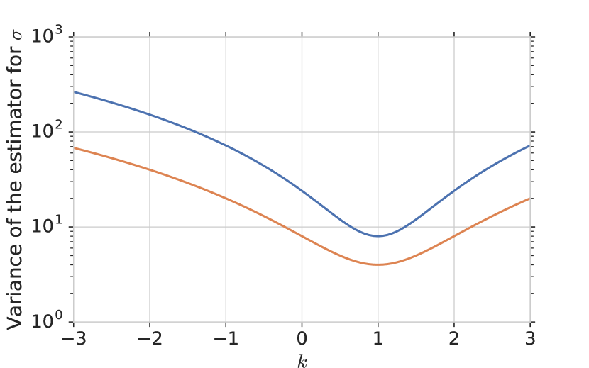

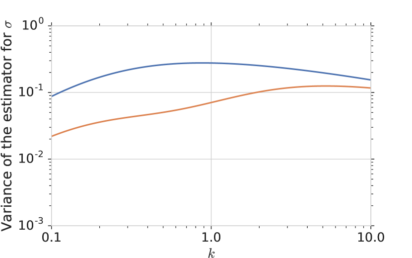


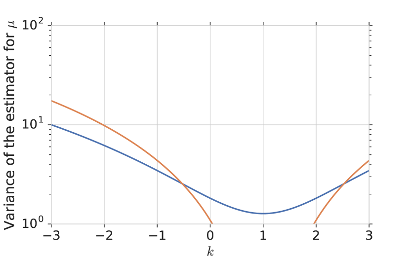

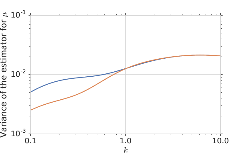

7.3 Variance Reduction by Conditioning
Probabilistically conditioning our estimators on a subset of dimensions and integrating out the remaining dimensions analytically is a powerful form of variance reduction in Monte Carlo estimators, sometimes referred to as Rao-Blackwellisation. Assume that the dimensions of are partitioned into a set and its complement with the expectation being analytically computable for all values of . We can then estimate by performing Monte Carlo integration over a smaller space of :
| (47) |
We can show that this conditional estimator has lower variance than its unconditional counterpart. Following Owen (2013), by the law of total variance, we have
| (48) | ||||
| (49) | ||||
| (50) |
which shows that the conditional system has lower variance than than the unconditional system . Thus the conditional estimator is guaranteed to have lower variance than unconditional one :
| (51) |
Conditioning is the basis of several variance reduction schemes: smoothed perturbation analysis for the pathwise derivative (Gong and Ho, 1987); the use of leave-one-out estimation and Rao-Blackwellisation in hierarchical models by Ranganath (2017); and the local-expectation gradients developed by Titsias and Lázaro-Gredilla (2015) to improve on the variance properties of score-function and pathwise estimators in variational inference.
This technique is useful in practice only if we can compute the conditional expectations involved efficiently, whether analytically or with numerical integration. If evaluating these expectations is costly, then simply increasing the number of samples in the Monte Carlo estimator over the original space may prove easier and at least as effective.
7.4 Control Variates
We now consider a general-purpose technique for reducing the variance of any Monte Carlo method, again looking at the general problem (1), which we can do since all the gradient estimators we developed in the preceding sections were eventually of this form. The strategy we will take is to replace the function in the expectation (1) by a substitute function whose expectation is the same, but whose variance is lower. If we have a function with a known expectation , we can easily construct such a substitute function along with the corresponding estimator as follows:
| (52) | |||
| (53) |
where and we use the shorthand and denote the sample averages. We refer to the function as a control variate, and the estimator (53) a control variate estimator. Control variates allow us to exploit information about quantities with known expectations, to reduce the variance of an estimate of an unknown expectation. The observed error serves as a control in estimating , and is a coefficient that affects the strength of the control variate. We expand on the specific choice of in Section 7.4.3. Glynn and Szechtman (2002) describe the connections between control variates and other variance reduction approaches such as antithetic and stratified sampling, conditional Monte Carlo, and non-parametric maximum likelihood.
7.4.1 Bias, Consistency and Variance
We can show that if the variance of is finite, both the unbiasedness and consistency of the estimator (53) are maintained:
| (54) | |||
| (55) |
Importantly, we can characterise the variance of the estimator (for ) as
| (56) |
By minimising (56) we can find that the optimal value of the coefficient is
| (57) |
where we expressed the optimal coefficient in terms of the variance of and , as well as in terms of the correlation coefficient . The effectiveness of the control variate can be characterised by the ratio of the variance of the control variate estimator to that of the original estimator: we can say our efforts have been effective if the ratio is substantially less than 1. Using the optimal control coefficient in (56), we find that the potential variance reduction is
| (58) |
Therefore, as long as and are not uncorrelated, we can always obtain a reduction in variance using control variates. However, for variance reduction to be substantial, we need control variates that are strongly correlated with the functions whose variance we wish to reduce. The sign of the correlation does not matter since it is absorbed into , and the stronger the correlation, the larger the reduction in variance.
In practice, the optimal will not be known and so we will usually need to estimate it empirically. Estimating using the same samples used to estimate will introduce a bias because and will no longer be independent. In practice, this bias is often small (Owen, 2013; Glasserman, 2013), and can be controlled since it decreases quickly as the number of samples is increased. This bias can also be eliminated by using a family of ‘splitting techniques’, as described by Avramidis and Wilson (1993). We refer to the discussion by Nelson (1990) for additional analysis on this topic.
7.4.2 Multiple and Non-linear Controls
The control variates in (52) are linear control variates, and this form should be used as a default. A first generalisation of this is in allowing for multiple controls, where we use a set of controls rather than one, using
| (59) |
where is now a -dimensional vector of coefficients, with usually kept low; the bias and variance analysis follows the single-control case above closely. The use of multiple controls is best suited to cases when the evaluation of the function is expensive and can be approximated by a linear combination of inexpensive control variates.
We can also consider non-linear ways of introducing control variates. Three alternative (multiplicative) forms are
| (60) |
These multiplicative controls lead to consistent but biased estimates. The non-linear controls also do not require a coefficient since this is implicitly determined by the relationship between and . When we use a large number of samples in the estimator, non-linear controls are no better than linear controls, since asymptotically it is the linear terms that matter (Glynn and Whitt, 1989, sect. 8). In most contemporary applications, we do not use large samples—often we use a single sample in the estimator—and it is in this small sample regime that non-linear controls may have applicability. The practical guidance though, remains to use linear controls as the default.
7.4.3 Designing Control Variates
The primary requirements for a control variate are that it must have a tractable expectation and, ideally, be strongly correlated with the target. While control variates are a very general technique that can be applied to any Monte Carlo estimator, designing effective control variates is an art, and the best control variates exploit the knowledge of the problem at hand. We can identify some general strategies for designing controls:
- Baselines.
-
One simple and general way to reduce the variance of a score-function gradient estimator is to use the score function itself as a control variate, since its expectation under the measure is zero (Equation (12)). This simplifies to subtracting the coefficient from the cost in the score function estimator in (13d), giving the modified estimator
(61) In reinforcement learning, is called a baseline (Williams, 1992) and has historically been estimated with a running average of the cost. While this approach is easier to implement than optimising to minimise variance, it is not optimal and does not guarantee lower variance compared to the vanilla score-function estimator (Weaver and Tao, 2001). Baselines are among the most popular variance reduction methods because they are easy to implement, computationally cheap, and require minimal knowledge about the problem being solved. We explore the baseline approach in an empirical analysis in Section 8.3.
- Bounds.
-
We can use bounds on the cost function as ways of specifying the form of the control variate . This is intuitive because it maintains a correlation between and , and if chosen well, may be easily integrable against the measure and available in closed form. This approach requires more knowledge of the cost function, since we will need to characterise the cost analytically in some way to bound it. Several bounding methods, such as Böhning and Jaakkola’s bounds (Khan et al., 2010), and piecewise bounds (Marlin et al., 2011), have been developed in local variational inference. Paisley et al. (2012) show specific use of bounds as control variates. In general, unless the bounds used are tight, they will not be effective as control variates, since the gap between the bound and the true function is not controllable and will not necessarily give the information needed for variance reduction.
- Delta Methods.
-
We can create control variates by approximating the cost function using a Taylor expansion. This requires a cost function that is differentiable so that we can compute the second-order Taylor expansion, but can be an effective and very general approach for variance reduction that allows easy implementation (Paisley et al., 2012; Owen, 2013). We will develop a specific example in Section 8.1.
- Learning Controls.
-
If we estimate the gradients repeatedly as a part of an optimisation process, we can create a parameterised control variate function and learn it as part of the overall optimisation algorithm. This allows us to create a control variate that dynamically adapts over the course of optimisation to help better match the changing nature of the cost function. Furthermore, this approach makes it easy to condition on any additional information that is relevant, e.g., by using a neural network to map the additional information to the parameters of the control variate. This strategy has been used by Mnih and Gregor (2014) to reduce the score-function gradient variance substantially in the context of variational inference, by defining the baseline as the output of a neural network that takes the observed data point as its input. This approach is general, since it does not make assumptions about the nature of the cost function, but introducing a new set of parameters for the control function can make the optimisation process more expensive.
Even in the simpler case of estimating the gradient only once, we can still learn a control variate that results in non-trivial variance reduction as long as we generate sufficiently many samples to train it and use a sample-efficient learning algorithm. Oates et al. (2017) demonstrated the feasibility of this approach using kernel-based non-parametric control variates.
8 Case Studies in Gradient Estimation
We now bring together the different approaches for gradient estimation in a set of case studies to explore how these ideas have been combined in practice. Because these gradients are so fundamental, they appear in all the major sub-areas of machine learning—in supervised, unsupervised, and reinforcement learning. Not all combinations that we can now think of using what we have reviewed have been explored, and the gaps we might find point to interesting topics for future work.
8.1 Delta Method Control Variates
This case study makes use of the delta method (Bickel and Doksum, 2015), which is a method for describing the asymptotic variance of a function of a random variable. By making use of Taylor expansions, the delta method allows us to design lower variance gradient estimators by using the differentiability, if available, of the cost function. It can be used for variance reduction in both the score-function estimator (Paisley et al., 2012) and the pathwise estimator (Miller et al., 2017), and shows us concretely one approach for designing control variates that was listed in Section 7.4.3.
We denote the gradient and Hessian of the cost function as and , respectively. The second-order Taylor expansion of a cost function expanded around point and its derivative are
| (62) | ||||
| (63) |
We can use this expansion directly as a control variate for the score-function estimator, following the approach we took to obtain Equation (52):
| (64a) | ||||
| (64b) | ||||
In the first line, we again wrote the control-variate form for a Monte Carlo gradient, and in the second line we wrote out the gradient using the score-function approach. This is the control variate that is proposed by Paisley et al. (2012, eq. (12)) for Monte Carlo gradient estimation in variational inference problems. In the Gaussian mean-field variational inference that Paisley et al. (2012) consider, the second term is known in closed-form and hence does not require Monte Carlo approximation. Like in Equation (59), is a multivariate control coefficient and is estimated separately.
With the increased popularity of the pathwise gradient estimator in machine learning, Miller et al. (2017) showed how delta method control variates can be used with pathwise estimation in the context of variational inference. The approach is not fundamentally different from that of Paisley et al. (2012), and we show here that they can be derived from each other. If we begin with Equation (64a) and instead apply the pathwise estimation approach, using a sampling path , we will obtain the gradient
| (65a) | ||||
| (65b) | ||||
| (65c) | ||||
The first line recalls the linear control variate definition (52) and expands it. In the second line, we use the LOTUS to reparameterise the expectation in terms of the sampling path and the base distribution , but again assume that the final term is known in closed-form and does not require stochastic approximation. In the final line (65c) we exchanged the order of integration and differentiation, and applied the chain rule to obtain the form of the gradient described by Miller et al. (2017), though from a different starting point.
As both Paisley et al. (2012) and Miller et al. (2017) demonstrate, we can achieve an appreciable variance reduction using the delta method, if we are able to exploit the generic differentiability of the cost function. Due to the widespread use of automatic differentiation, methods like these can be easily implemented and allow for a type of automatic control variate, since no manual derivation and implementation is needed.
8.2 Hybrids of Pathwise and Score Function Estimators
Decoupling of gradient estimation and sampling was an aspect of the pathwise estimator that we expanded upon in Section 5.3.1. This decoupling can be achieved in other ways than with implicit differentiation that we used previously, and we explore two other options in this section.
Up to this point, we have always required that the sampling path consists of a transformation and a corresponding base distribution that is independent of the parameters . In some cases, we might only be able to find a weaker sampling path that consists of a transformation and a parameter-dependent base distributions . In this setting, we will obtain a gradient estimator that is a hybrid of the pathwise and score-function estimators:
| (66a) | ||||
| (66b) | ||||
| (66c) | ||||
In the first line, we expanded the definition of the gradient-expectation under the new parameter-dependent base distribution and the path . In the second line, we applied the chain rule for differentiation, which results in two terms involving the gradient of the function and the gradient of the distribution. In the final line (66c), we apply the identity for score functions (11) to replace the gradient of the probability with the gradient of the log-probability, which leaves us with two terms that we recognise as the two major gradient estimators we have explored in this paper. We note that estimators for both terms in (66c) can incorporate variance reduction techniques such as control variates. We now explore two approaches that fit within this hybrid estimator framework.
8.2.1 Weak Reparameterisation
Sampling paths of the type we just described, which have parameter-dependent base distributions , are referred to by Ruiz et al. (2016) as weak reparameterisations.
Example (Gamma Weak Reparameterisation). The Gamma distribution with shape parameter and rate can be represented using the weak reparameterisation (Ruiz et al., 2016)
| (67a) | |||
| (67b) |
where is the digamma function, and is its derivative. The final density (67b) can be derived by using change of variable formula (27), and shows what is meant by weak dependency, since it depends on shape parameter but not on the rate parameter .
Using knowledge of the existence of a weak reparameterisation for the measure we can rewrite (66c). We use two shorthands: for the gradient of the weak-path with respect to the parameters, and for the gradient of the logarithm of the Jacobian-determinant. The pathwise term in (66c) becomes
| (68a) | ||||
| (68b) | ||||
| (68c) | ||||
where we first applied the rule for the change of variables to rewrite the integrals in terms of the variable . Introducing the infinitesimals for cancels the determinant terms, after which we apply the chain rule and finally rewrite it in the more familiar expectation form in the final line. Similarly, the score function term in (66c) can be written as
| (69a) | |||
| (69b) | |||
| (69c) | |||
where we again use the rule for the change of variables in the second line wherever appears. On the next line we enumerate the two ways in which depends on when computing the gradient w.r.t. . We obtain the final line by expressing the integral as an expectation w.r.t. , keeping in mind that .
8.2.2 Gradients with Rejection Sampling
Rejection sampling offers another way of exploring the decoupling of sampling from gradient estimation in pathwise estimation. Naesseth et al. (2017) developed the use of rejection sampling in the setting of the hybrid gradient (66c), which we will now present.
Using rejection sampling, we can always generate samples from a distribution using a proposal distribution for which for a finite constant . If we also know a parameterisation of the proposal distribution in terms of a sampling path and a base distribution , we can generate samples using a simple procedure: we repeat the three steps of drawing a sample , evaluating , and drawing a uniform variate , until , at which point we accept the corresponding as a sample from .
This algorithmic process of rejection sampling induces an effective base distribution
| (70) |
which intuitively reweights the original base distribution by the ratio of the measure and the proposal ; see Naesseth et al. (2017) for a detailed derivation. We can now reparameterise in our objective (1) using the proposal’s sampling path and the effective distribution (70):
| (71) |
The gradient (66c) can be rewritten using the effective distribution instead, giving another approach for gradient estimation:
| (72a) | |||
| (72b) | |||
To minimise the magnitude of the score-function term, the proposal distribution should be chosen so that it yield a high acceptance probability.
8.3 Empirical Comparisons
Logistic regression remains one of the most widely-used statistical models, and we use it here as a test case to explore the empirical performance of gradient estimators and to comment on their implementation and interactions with the optimisation procedure. Bayesian logistic regression defines a probabilistic model for a target given features (or covariates) for data points , using a set of parameters . We denote the collection of all data points as . Using a Gaussian prior on the parameters and a Bernoulli likelihood, the probabilistic model is
| (73) |
where is the logistic function, and is a constant. We use variational Bayesian logistic regression, an approximate Bayesian inference procedure, to determine the parameter posterior distribution (Jaakkola and Jordan, 1997; Murphy, 2012). Variational inference was one of the five research areas that we reviewed in Section 2 to which gradient estimation is of central importance, allows us to specify a bound on the integrated likelihood of the logistic regression model, maximising which requires gradients of the form of (2). Variational inference introduces a variational distribution , with variational parameters that are optimised using a variational lower bound objective (Jaakkola and Jordan, 1997)
| (74) |
The first expectation is a problem of the form we have studied throughout this paper, which is the expectation of a cost function, given by a log-likelihood under a Gaussian measure; and we are interested in Monte Carlo gradients of the variational parameters . The second term is the Kullback-Leibler (KL) divergence between the variational posterior and the prior distribution , which is known in closed-form for Gaussian distributions; in other models, the KL will not be known in closed-form, but its gradients can still be computed using the estimators we discuss in this paper. We optimise the variational bound using stochastic gradient descent, and compare learning of the variational parameters using both the score-function and pathwise estimator. The objective function we use is a Monte Carlo estimator of Equation (74):
| (75) | ||||
| (76) |
where is the data batch size, is the size of the full data set, is the number of samples taken from the posterior distribution to evaluate the Monte Carlo gradient, and the posterior covariance is a diagonal matrix . We use stochastic gradient descent for optimisation, with cosine learning rate decay (Loshchilov and Hutter, 2017) unless stated otherwise. We use the UCI Women’s Breast Cancer data set (Dua and Graff, 2017), which has data points and features. For evaluation, we always use the entire data set and posterior samples. Using this setup, we tie together the considerations raised in the previous sections, comparing gradient estimators when used in the same problem setting, looking at the interaction between the Monte Carlo estimation of the gradient and the mini-batch optimisation, and reporting on the variance of estimators under different variance reduction schemes. Generalised regression using the pathwise and score function estimators have been explored in several papers including Paisley et al. (2012); Kucukelbir et al. (2017); Salimans and Knowles (2013); Wang et al. (2013); Miller et al. (2017).
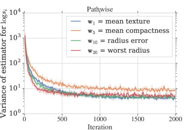
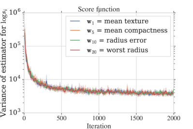
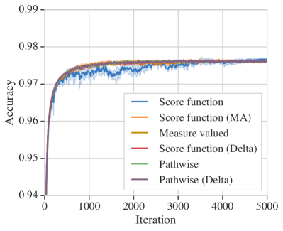
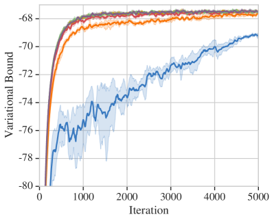
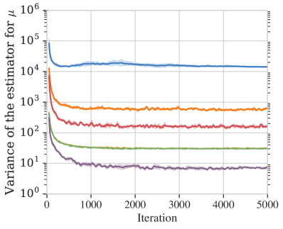
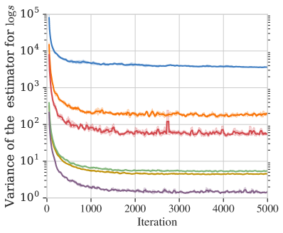
Decreasing variance over training.
Figure 8 shows the variance of the two estimators for the gradient with respect to the log of the standard deviation for four input features. These plots establish the basic behaviour of the optimisation: different dimensions have different gradient-variance levels; this variance decreases over the course of the optimisation as the parameters get closer to an optimum. The same behaviour is shown by both estimators, but the magnitude of the variance is very different between them, with the pathwise estimator having much lower variance compared to the score-function.
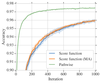
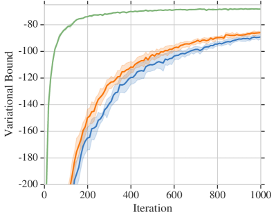
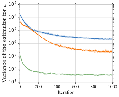
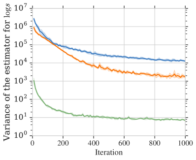
Performance with fixed hyperparameters.
We compare the score-function and pathwise estimators by now fixing the hyperparameters of the optimisation algorithm, using a batch size of data points, a learning rate of and estimating the gradient using samples from the measure. Figure 9 shows the variational lower bound and the accuracy that is attained in this setting. These graphs also show the control-variate forms of the gradient estimators. As control variates, we use the delta method (Section 8.1) and the moving average (MA) baseline (Section 7.4.3). For the delta method control variate, we always use 25 samples from the measure to estimate the control variate coefficient using Equation (57).
Comparing the different estimators in Figure 9, the pathwise estimator has lower variance and faster convergence than the score-function estimator. The score-function estimator greatly benefits from the use of control variates, with both the moving average baseline and the delta method reducing the variance. The delta method control variate leads to greater variance reduction than a moving average baseline, and reduces variance both for the score-function and pathwise estimators. We already have a sense from these plots that where the pathwise estimator is applicable, it forms a good default estimator since it achieves the same performance level but with lower variance and faster convergence.
Using fewer samples.
Figure 10 shows a similar setup to Figure 9, with a fixed batch size , but using fewer samples from the measure, . Using fewer samples affects the speed of convergence. The score-function estimator converges slower than the pathwise estimator, since it requires smaller learning rates. And like in the previous figure, this instability at higher learning rates can be addressed using more samples in the estimator, or more advanced variance reduction like the delta method.
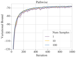
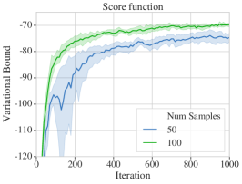
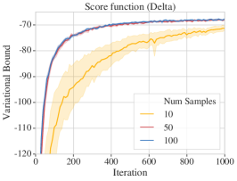
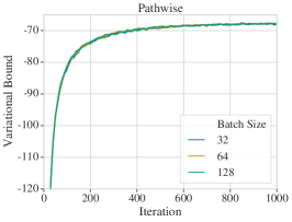
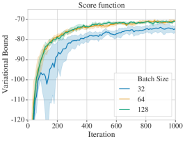
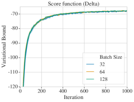
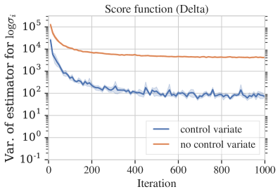
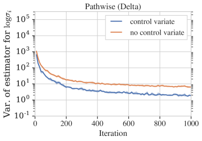
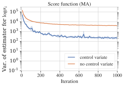
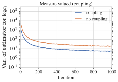
Effect of batch size and samples.
We now vary the number of samples from the measure that is used in computing the gradient estimator, and the batch size, and show the comparative performance in Figures 11 and 12. In Figure 11 there is a small change in the rate of the convergence of the pathwise estimator as the number of samples is increased. In contrast, the score-function estimator benefits much more from increasing the number of samples used. As the batch size is increased in Figure 12, we again see a limited gain for the pathwise estimator and more benefit for the score-function estimator.
When control variates are used with these estimators, the score-function estimator benefits less from an increase in the number posterior samples or an increase in batch size compared to the vanilla score-function estimator. The performance of the vanilla score-function estimator can match that of the score function estimator with a delta control variate, by increasing the number of posterior samples: using the score-function estimator matches the variational lower bound obtained by the score-function estimator with a delta control variate when . This exposes a trade-off between implementation complexity and sample efficiency.
Same number of function evaluations.
Figure 9 shows that the measure-valued estimator achieves the same variance as the pathwise estimator without making use of the gradient of the cost function. The measure-valued estimator outperforms the score-function estimator, even when a moving average baseline is used for variance reduction. This comes at a cost: the measure-valued estimator uses more function evaluations. To control for the cost, we also perform a comparison in which both methods use the same number of function evaluations by using more samples for the score-function estimator and show results in Figure 14. In this scenario, the vanilla score function still exhibits higher variance than the measure-valued estimator, but when augmented with a moving average baseline, which is a simple and computationally efficient variance reduction method, the score-function estimator performs best.
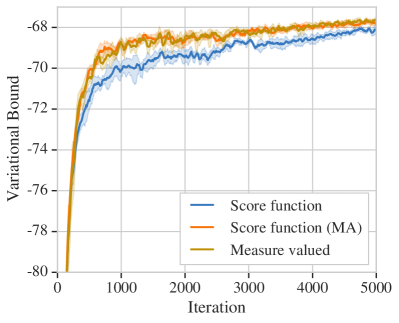
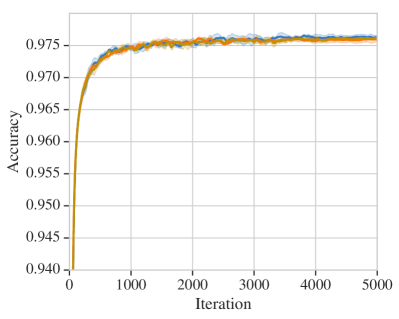
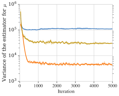
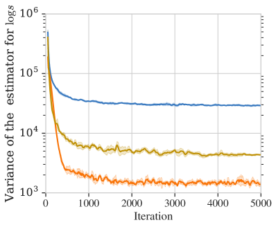
Controlling comparisons.
When working with control variates, we found it useful to record for each iteration what the gradient variance would have been for the current update had the control variate not been used, in order to check that variance reduction is working. We show the results in this regime for both pathwise and score-function estimators in Figure 13.
9 Discussion and Extensions
9.1 Testing Gradient Implementations
Implementing Monte Carlo gradient estimators can be an error-prone process, so it is important to verify the correctness of the implemented estimator. We consider unbiased gradient estimators, so a good check is to compare the Monte Carlo estimate using a large number of samples to the exact gradient in a test problem for which the analytic solution is known. As basic tests: if the mean of the measure is known, we can use ; if the covariance matrix of the measure is also known, we can pick . As an example, for the Gamma distribution , its mean is and the exact gradient . Then, we approximate the left hand side using Monte Carlo samples of a stochastic gradient estimator and compare the result to 1 with some tolerance, choosing samples is a good starting point.
It is also useful to check that, in expectation over a large number of samples, different unbiased estimators produce the same gradients for a variety of functions. With this approach, we can also use functions for which we do not know the exact gradient of the expectation. For methods that use control variates for variance reduction, it is useful to check that the stochastic estimates of the expectation of the control variate and its gradients are close to their analytically computed values. To assess the variance reduction effects of the control variate, it is useful to also track the variance for the gradient estimator without the control variate, like we do in Figure 13. These simple tests allow for a robust set of unit tests in code, to which more sophisticated testing methods can be added, e.g. the tests described by Geweke (2004). For all the tests accompanying our implementation of the stochastic gradient estimators described in this work, see the note on the code in the introduction.
9.2 Stochastic Computational Graphs and Probabilistic Programming.
Computational graphs (Bauer, 1974) are now the standard formalism with which we represent complex mathematical systems in practical systems, providing a modular tool with which to reason about the sequence of computations that transform a problem’s input variables into its outputs. A computational graph defines a directed acyclic graph that describes a sequence of computations, from inputs and parameters to final outputs and costs. This is the framework in which automatic differentiation systems operate. Computational graphs allow us to automatically track dependencies between individual steps within our computations and then, using this dependency structure, enable the sensitivity analysis of any parameters by backwards traversal of the graph (Griewank et al., 1989; Baydin et al., 2018). In standard computational graphs, all operations are represented by nodes that are deterministic, but in the problems that we have studied, some of these nodes will be random, giving rise to stochastic computational graphs.
Stochastic computational graphs provide a framework for implementing systems with both deterministic and stochastic components, and efficiently and automatically computing gradients using the types of estimators that we reviewed in this paper (Schulman et al., 2015; Kucukelbir et al., 2017). With such a framework it is easy to create complex probabilistic objects that mix differentiable and non-differentiable cost functions, and that use variables with complex dependencies. Simpler approaches for rich computational graphs of this type first approximate all intractable integrals using the Laplace approximation and apply automatic differentiation to the resulting approximation (Fournier et al., 2012). Stochastic variational message passing (Winn and Bishop, 2005; Paquet and Koenigstein, 2013) uses mean-field approximations, bounding methods, and natural parameterisations of the distributions involved, to create another type of stochastic computational graph that uses more detailed information about the structural properties of the cost and the measure. Seeking greater automation, Schulman et al. (2015) exploit the score-function and pathwise derivative estimators to automatically provide gradient estimates for non-differentiable and differentiable components of the graph, respectively.
The framework of Schulman et al. (2015), Kucukelbir et al. (2017), Fournier et al. (2012), Parmas (2018) and others, shows that it is easy to combine the score-function and pathwise estimators and automatically deploy them in situations where they are naturally applicable. This framework has been further expanded by incorporating methods that include variance reductions within the computational graph, and allowing higher-order gradients to be computed more easily and with lower variance (Weber et al., 2019; Foerster et al., 2018; Mao et al., 2018; Parmas et al., 2018). There are as yet no automated computational frameworks that include the measure-valued gradients. But as Pflug (1996) mentions, since the weak derivative—and also the sampling mechanism for the positive and negative density components—is known for most of distributions in common use (c.f. Table 1), it is possible to create a computational framework with sets of nodes that have knowledge of their corresponding weak derivatives to enable gradient computation. The score-function estimator is implemented in stochastic computational graphs using surrogate nodes and loss functions (c.f. Schulman et al. (2015)), and the measure-valued gradients could be realised through similar representations.
The framework of a stochastic computational graph enables us to more easily explore complex probabilistic systems, since we are freed from creating customised implementations for gradient estimation and optimisation. They also make it easier to develop probabilistic programming languages, that is programming languages in which we specify generative and probabilistic descriptions of systems and data, and then rely on automated methods for probabilistic inference. Many of the approaches for automated inference in probabilistic programs, like variational inference, rely on the automated computation of Monte Carlo gradient estimates (Wingate et al., 2011; Ritchie et al., 2016; Kucukelbir et al., 2017).
9.3 Gaussian Gradients
The case of Gaussian measures is a widely-encountered special case for gradient estimation. If we know we will be using a Gaussian then we can derive estimators that exploit its specific properties. Consider the multivariate Gaussian with mean and variance that are functions of parameters whose gradients we are interested in. The most common approach for gradient computation is by pathwise estimation using the location-scale transform for the Gaussian, with the decomposition :
where .
Alternatively, since we are dealing specifically with Gaussian measures, we can use the Bonnet’s theorem (Bonnet, 1964) and the Price’s theorem (Price, 1958; Rezende et al., 2014) to directly compute the gradient with respect to the Gaussian mean and covariance, respectively:
| (77) | |||
| (78) | |||
| (79) |
where and are the gradient and Hessian of the cost function . Using the Price’s theorem is computationally more expensive, since it requires evaluating the Hessian, which incurs a cubic computational cost, and will not be scalable in high-dimensional problems. By comparison, the location-scale path has linear cost in the number of parameters, but at the expense of higher variance.
We can also extend the Price’s theorem (78) to the second order (Fan et al., 2015):
| (80) |
where are indices on the dimensionality of the parameters space; is the th element of the covariance matrix and is the th element of the vector . This shows that while we can compute gradients in a form suitable for higher-order gradients, for Gaussian measures, this comes at the cost of needing up to 4th-order differentiability of the cost function.
9.4 Gradients Estimators using Optimal Transport
An interesting connection to the pathwise gradient estimators was identified by Jankowiak and Obermeyer (2018) using the tools of optimal transport. Because probabilities are themselves conserved quantities, we will find that the probabilities we use, as we vary their parameters, must satisfy the continuity equation (Santambrogio, 2015, sect. 4.1.2)
| (81) |
where is the divergence operator with respect to variables , and is a velocity field for the parameter ; there is a different velocity field for each parameter for . In univariate cases, the velocity field can be obtained by solving the continuity equation to obtain , where is the cumulative distribution function of ; also see Equation (33). Using this definition, the gradient (2) for the th parameter can be computed as
| (82) |
which can be derived by first interchanging the order of differentiation and integration, substituting the density derivative with the expression for the vector field given by the continuity equation and then simplifying the expression using the product rule for divergences. One immediate connection we see is that the solution for the velocity field is exactly the solution for the quantity that we identified in Equation (31c), when we use the cumulative distribution function as the inverse transformation (). The form of the gradient that is identified here was also derived in a very different way by Cong et al. (2019). In the multivariate case we can obtain a continuous set of solutions of the continuity equation and then select the one with the lowest variance (Jankowiak and Obermeyer, 2018; Jankowiak and Karaletsos, 2019). This set of solutions can be equivalently viewed as a set of control variates for the pathwise gradient. A deeper exploration of these connections, and the set of tools that they make available from other areas of mathematics, stands to provide us with many other approaches for gradient estimation.
9.5 Harmonic Gradient Estimators
We can add an additional class of gradient estimators to the set we considered by decomposing the stochastic gradient problem (2) in terms of a Fourier series, resulting in the frequency domain or harmonic gradient estimators (Vázquez-Abad and Jacobson, 1994; Jacobson and Schruben, 1999; Jacobson et al., 1986). The intuition for this estimator is that by oscillating the parameters of the input measures sinusoidally, we can, at different frequencies, observe the sensitivity (gradient) of the cost with respect to the parameters of interest.
The harmonic approach turns out to be an efficient way of implementing a weighted finite-difference method with sinusoidally varying step-sizes (Jacobson, 1994; Vázquez-Abad and Jacobson, 1994). This also connects us to many other weighted finite difference schemes that might be applicable for the problem of gradient estimation, e.g., (Fu et al., 2018). In the context of Monte Carlo gradient estimation, the difficulty in choosing the hyperparameters of the estimator (the so-called index, driving frequencies and oscillation amplitudes, Fu 1994) makes this the least generic of the estimators we have considered; it also has high computational complexity requiring many evaluations of the cost function e.g. (Fu et al., 2018). Despite the drawbacks of this construction, the general use of Fourier decompositions remains an interesting additional tool with which to exploit knowledge in our estimation problems.
9.6 Generalised Pathwise Gradients and Stein-type Estimators
In many statistical problems, the gradient of the entropy of a probabilistic model is an often required informational quantity:
| (83) |
where we first expanded the definition of the entropy, and then applied the chain rule. Here, the log probability takes the role of the cost function in our exposition. Equation (83) is an expression in the more familiar form that we encountered in the application of the pathwise estimator, particularly in the decoupling of sampling from gradient computation, whether using implicit differentiation (30b) or the continuity equation (82).
To apply the pathwise estimator, we must be able to differentiate the log-probability, which implies that it must be known. This will not always be the case, and one common setting where this is encountered in machine learning is when using likelihood-free or implicit probabilistic models (Mohamed and Lakshminarayanan, 2016). With implicit models, we can simulate data from a distribution, but do not know its log-probability. In such cases, the general strategy we take is to use a substitute function that fills the role of the unknown cost function, like the unknown log-probability, and that gives the gradient information we need, e.g. like the use of a classifier in generative adversarial networks (Goodfellow et al., 2014) or a moment network in the method of moments (Ravuri et al., 2018). In this way, we can create a more general pathwise estimator that can be used when the gradient of the cost function is unknown, but that will reduce to the familiar pathwise estimator from Section 5 when it is. Stein’s identity gives us a general tool with which to do this.
Stein’s identity (Gorham and Mackey, 2015; Liu et al., 2016) tells us that if a distribution is continuously differentiable then the gradient of its log-probability with respect to the random variable can be related to the gradient of a test function by the integral
| (84) |
We assume that test function has dimension , the random variable has dimension , and that is in the Stein class of defined by Gorham and Mackey (2015). By inverting this expression, we can find a general method for evaluating the gradient of a log probability. This expression is applicable to both normalised and unnormalised distributions, making it very general, i.e. we can use Stein’s identity to provide the unknown component . By expanding Stein’s identity as a Monte Carlo estimator and using several samples, Li and Turner (2017) use kernel substitution to develop a kernelised method for gradient estimation in implicit probabilistic models. They also provide the connections to other methods for estimating gradients of log-probabilities, such as score-matching and denoising auto-encoders. An alternative Stein-type gradient estimator using the spectral decomposition of kernels was developed by Shi et al. (2018), and Stein’s identity was also used in variational inference by Ranganath et al. (2016).
9.7 Generalised Score Functions and Malliavin-weighted Estimators
Stein’s identity gave us a tool with which to develop generalised pathwise estimators, and in a similar vein we can create a generalised score-function estimator. There are many problems where the explicit form of the density needed to compute the score is not known, such as when the density is defined by a continuous-time system or an implicit probabilistic model. In such cases, a generalised form of the score-function estimator (13c) is , i.e. the expected value of the cost function multiplied by a weighting function . When the weighting function is the score function, we will recover the score-function gradient, and in other cases, it gives us the information needed about the unknown score.
One approach for developing generalised score-function estimators that is widely used for continuous-time systems in computational finance is through Malliavin calculus, which is the calculus of variations for stochastic processes (Nualart, 2006). Computational finance provides one example of a setting where we do not know the density explicitly, because the random variables are instead specified as a diffusion process. The generalised gradient method based on weighting functions, called Malliavin weights, allows gradients to be computed in such settings, where the score function is replaced by a Skorokhod integral (Chen and Glasserman, 2007). There are equivalent concepts of differentiation (Malliavin derivative) and integration (Skorokhod integration) that allow for the interchange of differentiation and integration and the development of unbiased estimators in such settings. We defer to the papers by Fournié et al. (1999) and Benhamou (2003) in computational finance, and, closer to machine learning, the papers by Gobet and Munos (2005) and Munos (2006) in optimal control and reinforcement learning for further exploration of these ideas.
9.8 Discrete Distributions
We purposefully limited the scope of this paper to measures that are continuous distributions in their domain. There are many problems, such as those with discrete latent variables and in combinatorial optimisation, where the measure will instead be a discrete distribution, such as the Bernoulli or Categorical. This is a large area of research in itself, but does have some overlap with our coverage in this paper. While the Bernoulli or Categorical are discrete distributions over their domain, they are continuous with respect to their parameters, which means that both the score-function estimator and the measure-valued derivative are applicable to such estimation problems. Coverage of this discrete distribution setting makes for an interesting review paper in itself, and existing work includes Tucker et al. (2017); Maddison et al. (2016); Mnih and Gregor (2014); Gu et al. (2016); Glasserman and Ho (1991).
10 Conclusion
We have been through a journey of more than fifty years of research in one of the fundamental problems of the computational sciences: computing the gradient of an expectation of a function. We found that this problem lies at the core of many applications with real-world impact, and a broad swathe of research areas; in applied statistics, queueing theory, machine learning, computational finance, experimental design, optimal transport, continuous-time stochastic processes, variational inference, reinforcement learning, Fourier analysis, causal inference, and representation learning, amongst many others subjects. The gradients in all these areas fall into one of two classes, gradients-of-measure or gradients-of-paths. We derived the score-function estimator and the measure-valued gradient estimator as instances of gradients of measure, both of which exploit the measure in the stochastic objective to derive the gradient. And we derived the pathwise estimator that uses knowledge of the sampling path to obtain the gradient. All these methods benefit from variance reduction techniques and we reviewed approaches for variance reduction we might consider in practice. We further explored the use of these estimators through a set of case studies, and explored some of the other tools for gradient estimation that exist beyond the three principal estimators.
10.1 Guidance in Choosing Gradient Estimators
With so many competing approaches, we offer our rules of thumb in choosing an estimator, which follow the intuition we developed throughout the paper:
-
•
If our estimation problem involves continuous functions and measures that are continuous in the domain, then using the pathwise estimator is a good default. It is relatively easy to implement and its default implementation, without additional variance reduction, will typically have variance that is low enough so as not to interfere with the optimisation.
-
•
If the cost function is not differentiable or is a black-box function then the score-function or the measure-valued gradients are available. If the number of parameters is low, then the measure-valued gradient will typically have lower variance and would be preferred. But if we have a high-dimensional parameter set, then the score-function estimator should be used.
-
•
If we have no control over the number of times we can evaluate a black-box cost function, effectively only allowing a single evaluation of it, then the score function is the only estimator of the three we reviewed that is applicable.
-
•
The score-function estimator should, by default, always be implemented with at least some basic variance reduction. The simplest option is to use a baseline control variate estimated with a running average of the cost value.
-
•
When using the score-function estimator, some attention should be paid to the dynamic range of the cost function and its variance, and ways found to keep its value bounded within a reasonable range, e.g. by transforming the cost so that it is zero mean, or using a baseline.
-
•
For all estimators, track the variance of the gradients if possible and address high variance by using a larger number of samples from the measure, decreasing the learning rate, or clipping the gradient values. It may also be useful to restrict the range of some parameters to avoid extreme values, e.g. by clipping them to a desired interval.
-
•
The measure-valued gradient should be used with some coupling method for variance reduction. Coupling strategies that exploit relationships between the positive and negative components of the density decomposition, and which have shared sampling paths, are known for the commonly-used distributions.
-
•
If we have several unbiased gradient estimators, a convex combination of them might have lower variance than any of the individual estimators.
-
•
If the measure is discrete on its domain then the score-function or measure-valued gradient are available. The choice will again depend on the dimensionality of the parameter space.
-
•
In all cases, we strongly recommend having a broad set of tests to verify the unbiasedness of the gradient estimator when implemented.
10.2 Future Work
With all the progress in gradient estimation that we have covered, there still remain many more directions for future work, and there is still the need for new types of gradient estimators. Gradient estimators for situations where we know the measure explicitly, or only implicitly though a diffusion, are needed. New tools for variance reduction are needed, especially in more complex systems like Markov processes. The connections between the score function and importance sampling remains to be more directly related, especially with variance reduction in mind. Coupling was a tool for variance reduction that we listed, and further exploration of its uses will prove fruitful. And there remain opportunities to combine our existing estimators to obtain more accurate and lower variance gradients. The measure-valued derivatives have not been applied in machine learning, and it will be valuable to understand the settings in which they might prove beneficial. Gradient estimators for continuous-time settings like the Malliavin-weighted versions, multivariate estimators derived using optimal transport, the use of non-linear control covariates, the use of higher-order gradients, variants using the natural gradient and information geometry, and the utility of Fourier series are among many of the other questions that remain open.
Good gradients lead to ever-more interesting applications; ultimately, there remains much more to do in advancing the principles and practice of Monte Carlo gradient estimation.
Acknowledgements
We thank the action editor and our anonymous reviewers for their feedback. We are also grateful to many of our colleagues for their invaluable feedback during the preparation of this paper. In particular, we would like to thank Michalis Titsias, Cyprien de Masson d’Autume, Csaba Cspesvari, Fabio Viola, Suman Ravuri, Arnaud Doucet, Nando de Freitas, Ulrich Paquet, Danilo Rezende, Theophane Weber, Dan Horgan, Jonas Degrave, Marc Deisenroth, and Louise Deason. Finally, we thank many from the wider machine learning community who sent us points of improvement and requests for clarifications that strengthened this paper greatly.
A Common Distributions
The following table provides the definitions of the distributions that were mentioned within the paper.
| Name | Domain | Notation | Probability Density/Mass Function |
|---|---|---|---|
| Gaussian | |||
| Double-sided Maxwell | |||
| Weibull | |||
| Poisson | |||
| Erlang | |||
| Gamma | |||
| Exponential |
References
- Alemi et al. (2017) A. A. Alemi, I. Fischer, J. V. Dillon, and K. Murphy. Deep variational information bottleneck. In International Conference on Learning Representations, 2017.
- Avramidis and Wilson (1993) A. N. Avramidis and J. R. Wilson. A splitting scheme for control variates. Operations Research Letters, 14(4):187–198, 1993.
- Bauer (1974) F. L. Bauer. Computational graphs and rounding error. SIAM Journal on Numerical Analysis, 11(1):87–96, 1974.
- Baydin et al. (2018) A. G. Baydin, B. A. Pearlmutter, A. A. Radul, and J. M. Siskind. Automatic differentiation in machine learning: A survey. Journal of Machine Learning Research, 18:1–43, 2018.
- Bengio et al. (2014) Y. Bengio, E. Laufer, G. Alain, and J. Yosinski. Deep generative stochastic networks trainable by backprop. In International Conference on Machine Learning, 2014.
- Benhamou (2003) E. Benhamou. Optimal Malliavin weighting function for the computation of the Greeks. Mathematical Finance: An International Journal of Mathematics, Statistics and Financial Economics, 13(1):37–53, 2003.
- Bickel and Doksum (2015) P. J. Bickel and K. A. Doksum. Mathematical Statistics: Basic Ideas and Selected Topics, Volume I. CRC Press, 2015.
- Billingsley (2008) P. Billingsley. Probability and Measure. John Wiley & Sons, 2008.
- Blei et al. (2017) D. M. Blei, A. Kucukelbir, and J. D. McAuliffe. Variational inference: A review for statisticians. Journal of the American Statistical Association, 112(518):859–877, 2017.
- Bonnet (1964) G. Bonnet. Transformations des signaux aléatoires a travers les systemes non linéaires sans mémoire. Annales des Télécommunications, 19:203–220, 1964.
- Buchholz et al. (2018) A. Buchholz, F. Wenzel, and S. Mandt. Quasi-Monte Carlo variational inference. In International Conference on Machine Learning, 2018.
- Buesing et al. (2016) L. Buesing, T. Weber, and S. Mohamed. Stochastic gradient estimation with finite differences. In NeurIPS Workshop on Advances in Approximate Inference, 2016.
- Capriotti (2008) L. Capriotti. Reducing the variance of likelihood ratio Greeks in Monte Carlo. In Winter Simulation Conference, 2008.
- Cassandras and Lafortune (2009) C. G. Cassandras and S. Lafortune. Introduction to Discrete Event Systems. Springer Science & Business Media, 2009.
- Chaloner and Verdinelli (1995) K. Chaloner and I. Verdinelli. Bayesian experimental design: A review. Statistical Science, 10:273–304, 1995.
- Chen and Glasserman (2007) N. Chen and P. Glasserman. Malliavin Greeks without Malliavin calculus. Stochastic Processes and their Applications, 117(11):1689–1723, 2007.
- Chriss (1996) N. Chriss. Black Scholes and Beyond: Option Pricing Models. McGraw-Hill, 1996.
- Cong et al. (2019) Y. Cong, M. Zhao, K. Bai, and L. Carin. GO gradient for expectation-based objectives. In International Conference on Learning Representations, 2019.
- Deisenroth et al. (2013) M. P. Deisenroth, G. Neumann, and J. Peters. A Survey on Policy Search for Robotics, volume 2. Now Publishers, Inc., 2013.
- Devroye (1996) L. Devroye. Random variate generation in one line of code. In Winter simulation Conference, 1996.
- Devroye (2006) L. Devroye. Nonuniform random variate generation. Elsevier, 2006.
- Dua and Graff (2017) D. Dua and C. Graff. UCI machine learning repository, 2017. URL http://archive.ics.uci.edu/ml.
- Eslami et al. (2018) S. A. Eslami, D. J. Rezende, F. Besse, F. Viola, A. S. Morcos, M. Garnelo, A. Ruderman, A. A. Rusu, I. Danihelka, K. Gregor, et al. Neural scene representation and rendering. Science, 360(6394):1204–1210, 2018.
- Fan et al. (2015) K. Fan, Z. Wang, J. Beck, J. Kwok, and K. A. Heller. Fast second order stochastic backpropagation for variational inference. In Advances in Neural Information Processing Systems, 2015.
- Figurnov et al. (2018) M. Figurnov, S. Mohamed, and A. Mnih. Implicit reparameterization gradients. In Advances in Neural Information Processing Systems, 2018.
- Flanders (1973) H. Flanders. Differentiation under the integral sign. The American Mathematical Monthly, 80(6):615–627, 1973.
- Foerster et al. (2018) J. Foerster, G. Farquhar, M. Al-Shedivat, T. Rocktäschel, E. P. Xing, and S. Whiteson. DiCE: The infinitely differentiable Monte Carlo estimator. In International Conference on Machine Learning, 2018.
- Fournié et al. (1999) E. Fournié, J.-M. Lasry, J. Lebuchoux, P.-L. Lions, and N. Touzi. Applications of Malliavin calculus to Monte Carlo methods in finance. Finance and Stochastics, 3(4):391–412, 1999.
- Fournier et al. (2012) D. A. Fournier, H. J. Skaug, J. Ancheta, J. Ianelli, A. Magnusson, M. N. Maunder, A. Nielsen, and J. Sibert. AD model builder: Using automatic differentiation for statistical inference of highly parameterized complex nonlinear models. Optimization Methods & Software, 27(2):233–249, 2012.
- Fu (1994) M. C. Fu. Optimization via simulation: A review. Annals of Operations Research, 53(1):199–247, 1994.
- Fu and Hu (1993) M. C. Fu and J.-Q. Hu. Second derivative sample path estimators for the GI/G/M queue. Management Science, 39(3):359–383, 1993.
- Fu and Hu (2012) M. C. Fu and J.-Q. Hu. Conditional Monte Carlo: Gradient estimation and optimization applications. Springer Science & Business Media, 2012.
- Fu et al. (2018) M. C. Fu, B. Heidergott, H. Leahu, and F. Vazquez-Abad. Differentiation via logarithmic expansions. Asia-Pacific Journal of Operational Research, 2018.
- Geweke (2004) J. Geweke. Getting it right: Joint distribution tests of posterior simulators. Journal of the American Statistical Association, 99(467):799–804, 2004.
- Glasserman (2013) P. Glasserman. Monte Carlo Methods in Financial Engineering. Springer Science & Business Media, 2013.
- Glasserman and Ho (1991) P. Glasserman and Y. C. Ho. Gradient estimation via Perturbation Analysis. Springer Science & Business Media, 1991.
- Glynn (1987) P. W. Glynn. Likelilood ratio gradient estimation: An overview. In Winter simulation Conference, 1987.
- Glynn (1990) P. W. Glynn. Likelihood ratio gradient estimation for stochastic systems. Communications of the ACM, 33(10):75–84, 1990.
- Glynn and Iglehart (1989) P. W. Glynn and D. L. Iglehart. Importance sampling for stochastic simulations. Management Science, 35(11):1367–1392, 1989.
- Glynn and L’Ecuyer (1995) P. W. Glynn and P. L’Ecuyer. Likelihood ratio gradient estimation for stochastic recursions. Advances in applied probability, 27(4):1019–1053, 1995.
- Glynn and Szechtman (2002) P. W. Glynn and R. Szechtman. Some new perspectives on the method of control variates. In Monte Carlo and Quasi-Monte Carlo Methods 2000, pages 27–49. Springer, 2002.
- Glynn and Whitt (1989) P. W. Glynn and W. Whitt. Indirect estimation via . Operations Research, 37(1):82–103, 1989.
- Gobet and Munos (2005) E. Gobet and R. Munos. Sensitivity analysis using Itô–Malliavin calculus and martingales, and application to stochastic optimal control. SIAM Journal on Control and Optimization, 43(5):1676–1713, 2005.
- Gong and Ho (1987) W.-B. Gong and Y. C. Ho. Smoothed (conditional) perturbation analysis of discrete event dynamical systems. IEEE Transactions on Automatic Control, 32(10):858–866, 1987.
- Goodfellow et al. (2014) I. Goodfellow, J. Pouget-Abadie, M. Mirza, B. Xu, D. Warde-Farley, S. Ozair, A. Courville, and Y. Bengio. Generative adversarial nets. In Advances in Neural Information Processing Systems, 2014.
- Gorham and Mackey (2015) J. Gorham and L. Mackey. Measuring sample quality with Stein’s method. In Advances in Neural Information Processing Systems, pages 226–234, 2015.
- Gouriéroux and Monfort (1996) C. Gouriéroux and A. Monfort. Simulation-based Econometric Methods. Oxford University Press, 1996.
- Graves (2016) A. Graves. Stochastic backpropagation through mixture density distributions. arXiv:1607.05690, 2016.
- Greensmith et al. (2004) E. Greensmith, P. L. Bartlett, and J. Baxter. Variance reduction techniques for gradient estimates in reinforcement learning. Journal of Machine Learning Research, 5:1471–1530, 2004.
- Griewank et al. (1989) A. Griewank et al. On automatic differentiation. Mathematical Programming: Recent Developments and Applications, 6(6):83–107, 1989.
- Grimmett and Stirzaker (2001) G. Grimmett and D. Stirzaker. Probability and Random Processes. Oxford University Press, 2001.
- Gu et al. (2016) S. Gu, S. Levine, I. Sutskever, and A. Mnih. MuProp: Unbiased backpropagation for stochastic neural networks. In International Conference on Learning Representations, 2016.
- Hartford et al. (2016) J. Hartford, G. Lewis, K. Leyton-Brown, and M. Taddy. Counterfactual prediction with deep instrumental variables networks. In International Conference on Machine Learning, 2016.
- Heess et al. (2015) N. Heess, G. Wayne, D. Silver, T. Lillicrap, T. Erez, and Y. Tassa. Learning continuous control policies by stochastic value gradients. In Advances in Neural Information Processing Systems, 2015.
- Heidelberger et al. (1988) P. Heidelberger, X.-R. Cao, M. A. Zazanis, and R. Suri. Convergence properties of infinitesimal perturbation analysis estimates. Management Science, 34(11):1281–1302, 1988.
- Heidergott and Leahu (2010) B. Heidergott and H. Leahu. Weak differentiability of product measures. Mathematics of Operations Research, 35(1):27–51, 2010.
- Heidergott and Vázquez-Abad (2000) B. Heidergott and F. Vázquez-Abad. Measure-valued differentiation for stochastic processes: The finite horizon case. In EURANDOM report 2000-033, 2000.
- Heidergott et al. (2003) B. Heidergott, G. Pflug, and F. Vázquez-Abad. Measure-valued differentiation for stochastic systems: From simple distributions to Markov chains. 2003.
- Heidergott et al. (2008) B. Heidergott, F. J. Vázquez-Abad, and W. Volk-Makarewicz. Sensitivity estimation for Gaussian systems. European Journal of Operational Research, 187(1):193–207, 2008.
- Higgins et al. (2017) I. Higgins, L. Matthey, A. Pal, C. Burgess, X. Glorot, M. Botvinick, S. Mohamed, and A. Lerchner. Beta-VAE: Learning basic visual concepts with a constrained variational framework. In International Conference on Learning Representations, 2017.
- Ho and Cao (1983) Y. Ho and X. Cao. Optimization and perturbation analysis of queueing networks. Journal of Optimization Theory and Applications, 40(4):559–582, 1983.
- Ho and Cao (2012) Y. C. L. Ho and X. R. Cao. Perturbation analysis of discrete event dynamic systems, volume 145. Springer Science & Business Media, 2012.
- Hoffman and Blei (2015) M. Hoffman and D. Blei. Stochastic structured variational inference. In International Conference on Artificial Intelligence and Statistics, 2015.
- Honkela and Valpola (2004) A. Honkela and H. Valpola. Variational learning and bits-back coding: An information-theoretic view to Bayesian learning. IEEE Transactions on Neural Networks, 15(4):800–810, 2004.
- Hu et al. (2016) X. Hu, L. Prashanth, A. György, and C. Szepesvári. (Bandit) Convex optimization with biased noisy gradient oracles. In International Conference on Artificial Intelligence and Statistics, 2016.
- Jaakkola and Jordan (1997) T. Jaakkola and M. Jordan. A variational approach to Bayesian logistic regression models and their extensions. In International Conference on Artificial Intelligence and Statistics, 1997.
- Jacobson et al. (1986) S. Jacobson, A. Buss, and L. Schruben. Driving frequency selection for frequency domain simulation experiments. Technical report, Cornell University Operations Research and Industrial Engineering, 1986.
- Jacobson (1994) S. H. Jacobson. Optimal mean squared error analysis of the harmonic gradient estimators. Journal of Optimization Theory and Applications, 80(3):573–590, 1994.
- Jacobson and Schruben (1999) S. H. Jacobson and L. Schruben. A harmonic analysis approach to simulation sensitivity analysis. IIE Transactions, 31(3):231–243, 1999.
- Jankowiak and Karaletsos (2019) M. Jankowiak and T. Karaletsos. Pathwise derivatives for multivariate distributions. In International Conference on Artificial Intelligence and Statistics, 2019.
- Jankowiak and Obermeyer (2018) M. Jankowiak and F. Obermeyer. Pathwise derivatives beyond the reparameterization trick. In International Conference on Machine Learning, 2018.
- Jordan et al. (1999) M. I. Jordan, Z. Ghahramani, T. S. Jaakkola, and L. K. Saul. An introduction to variational methods for graphical models. Machine learning, 37(2):183–233, 1999.
- Kapuscinski and Tayur (1999) R. Kapuscinski and S. Tayur. Optimal policies and simulation-based optimization for capacitated production inventory systems. In Quantitative Models for Supply Chain Management, pages 7–40. Springer, 1999.
- Khan et al. (2010) M. E. Khan, G. Bouchard, K. P. Murphy, and B. M. Marlin. Variational bounds for mixed-data factor analysis. In Advances in Neural Information Processing Systems, 2010.
- Kingma and Welling (2014a) D. Kingma and M. Welling. Efficient gradient-based inference through transformations between Bayes nets and neural nets. In International Conference on Machine Learning, 2014a.
- Kingma and Welling (2014b) D. P. Kingma and M. Welling. Auto-encoding variational Bayes. In International Conference on Learning Representations, 2014b.
- Kleijnen and Rubinstein (1996) J. P. Kleijnen and R. Y. Rubinstein. Optimization and sensitivity analysis of computer simulation models by the score function method. European Journal of Operational Research, 88(3):413–427, 1996.
- Kucukelbir et al. (2017) A. Kucukelbir, D. Tran, R. Ranganath, A. Gelman, and D. M. Blei. Automatic differentiation variational inference. Journal of Machine Learning Research, 18(1):430–474, 2017.
- Kushner and Yin (2003) H. Kushner and G. G. Yin. Stochastic Approximation and Recursive Algorithms and Applications, volume 35. Springer Science & Business Media, 2003.
- Kusner et al. (2017) M. J. Kusner, B. Paige, and J. M. Hernández-Lobato. Grammar variational autoencoder. In International Conference on Machine Learning, 2017.
- L’Ecuyer (1995) P. L’Ecuyer. Note: On the interchange of derivative and expectation for likelihood ratio derivative estimators. Management Science, 41(4):738–747, 1995.
- Lee et al. (2018) W. Lee, H. Yu, and H. Yang. Reparameterization gradient for non-differentiable models. In Advances in Neural Information Processing Systems, 2018.
- Lehmann and Casella (2006) E. L. Lehmann and G. Casella. Theory of Point Estimation. Springer Science & Business Media, 2006.
- Leobacher and Pillichshammer (2014) G. Leobacher and F. Pillichshammer. Introduction to Quasi-Monte Carlo Integration and Applications. Springer, 2014.
- Li and Turner (2017) Y. Li and R. E. Turner. Gradient estimators for implicit models. In International Conference on Learning Representations, 2017.
- Lillicrap et al. (2016) T. P. Lillicrap, J. J. Hunt, A. Pritzel, N. Heess, T. Erez, Y. Tassa, D. Silver, and D. Wierstra. Continuous control with deep reinforcement learning. In International Conference on Learning Representations, 2016.
- Liu et al. (2016) Q. Liu, J. Lee, and M. Jordan. A kernelized Stein discrepancy for goodness-of-fit tests. In International Conference on Machine Learning, 2016.
- Loshchilov and Hutter (2017) I. Loshchilov and F. Hutter. SGDR: Stochastic gradient descent with warm restarts. In International Conference on Learning Representations, 2017.
- Maddison et al. (2016) C. J. Maddison, A. Mnih, and Y. W. Teh. The Concrete distribution: A continuous relaxation of discrete random variables. In International Conference on Learning Representations, 2016.
- Mao et al. (2018) J. Mao, J. Foerster, T. Rocktäschel, M. Al-Shedivat, G. Farquhar, and S. Whiteson. A baseline for any order gradient estimation in stochastic computation graphs. In International Conference on Machine Learning, 2018.
- Mark and Baram (2001) Z. Mark and Y. Baram. The bias-variance dilemma of the Monte Carlo method. In International Conference on Artificial Neural Networks, 2001.
- Marlin et al. (2011) B. M. Marlin, M. E. Khan, and K. P. Murphy. Piecewise bounds for estimating Bernoulli-logistic latent Gaussian models. In International Conference on Machine Learning, 2011.
- Metropolis and Ulam (1949) N. Metropolis and S. Ulam. The Monte Carlo method. Journal of the American Statistical Association, 44(247):335–341, 1949.
- Miller et al. (2017) A. Miller, N. Foti, A. D’Amour, and R. P. Adams. Reducing reparameterization gradient variance. In Advances in Neural Information Processing Systems, 2017.
- Miller (1967) L. B. Miller. Monte Carlo analysis of reactivity coefficients in fast reactors general theory and applications. Technical report, Argonne National Laboratory, 1967.
- Mnih and Gregor (2014) A. Mnih and K. Gregor. Neural variational inference and learning in belief networks. In Advances in Neural Information Processing Systems, 2014.
- Mohamed and Lakshminarayanan (2016) S. Mohamed and B. Lakshminarayanan. Learning in implicit generative models. arXiv:1610.03483, 2016.
- Munos (2006) R. Munos. Policy gradient in continuous time. Journal of Machine Learning Research, 7:771–791, 2006.
- Murphy (2012) K. P. Murphy. Machine Learning: A Probabilistic Perspective. MIT Press, 2012.
- Naesseth et al. (2017) C. Naesseth, F. Ruiz, S. Linderman, and D. Blei. Reparameterization gradients through acceptance-rejection sampling algorithms. In International Conference on Artificial Intelligence and Statistics, 2017.
- Nelson (1990) B. L. Nelson. Control variate remedies. Operations Research, 38(6):974–992, 1990.
- Newell (2013) C. Newell. Applications of Queueing Theory. Springer Science & Business Media, 2013.
- Nualart (2006) D. Nualart. The Malliavin Calculus and Related Topics. Springer, 2006.
- Oates et al. (2017) C. J. Oates, M. Girolami, and N. Chopin. Control functionals for Monte Carlo integration. Journal of the Royal Statistical Society: Series B (Statistical Methodology), 79(3):695–718, 2017.
- Opper and Archambeau (2009) M. Opper and C. Archambeau. The variational Gaussian approximation revisited. Neural Computation, 21(3):786–792, 2009.
- Owen (2013) A. B. Owen. Monte Carlo theory, methods and examples. 2013.
- Paisley et al. (2012) J. Paisley, D. Blei, and M. Jordan. Variational Bayesian inference with stochastic search. International Conference in Machine Learning, 2012.
- Papaspiliopoulos et al. (2007) O. Papaspiliopoulos, G. O. Roberts, and M. Sköld. A general framework for the parametrization of hierarchical models. Statistical Science, 22(1):59–73, 2007.
- Paquet and Koenigstein (2013) U. Paquet and N. Koenigstein. One-class collaborative filtering with random graphs. In International Conference on World Wide Web, 2013.
- Parmas (2018) P. Parmas. Total stochastic gradient algorithms and applications in reinforcement learning. In Advances in Neural Information Processing Systems, 2018.
- Parmas et al. (2018) P. Parmas, C. E. Rasmussen, J. Peters, and K. Doya. PIPPS: Flexible model-based policy search robust to the curse of chaos. In International Conference on Machine Learning, 2018.
- Pflug (1989) G. C. Pflug. Sampling derivatives of probabilities. Computing, 42(4):315–328, 1989.
- Pflug (1996) G. C. Pflug. Optimization of Stochastic Models: The Interface between Simulation and Optimization. Springer Science & Business Media, 1996.
- Price (1958) R. Price. A useful theorem for nonlinear devices having Gaussian inputs. IRE Transactions on Information Theory, 4(2):69–72, 1958.
- Ranganath (2017) R. Ranganath. Black Box Variational Inference: Scalable, Generic Bayesian Computation and its Applications. PhD thesis, Princeton University, 2017.
- Ranganath et al. (2014) R. Ranganath, S. Gerrish, and D. Blei. Black box variational inference. In International Conference on Artificial Intelligence and Statistics, 2014.
- Ranganath et al. (2016) R. Ranganath, D. Tran, J. Altosaar, and D. Blei. Operator variational inference. In Advances in Neural Information Processing Systems, 2016.
- Ravuri et al. (2018) S. Ravuri, S. Mohamed, M. Rosca, and O. Vinyals. Learning implicit generative models with the method of learned moments. In International Conference on Machine Learning, 2018.
- Reiman and Weiss (1989) M. I. Reiman and A. Weiss. Sensitivity analysis for simulations via likelihood ratios. Operations Research, 37(5):830–844, 1989.
- Rezende and Mohamed (2015) D. Rezende and S. Mohamed. Variational inference with normalizing flows. In International Conference on Machine Learning, 2015.
- Rezende et al. (2014) D. J. Rezende, S. Mohamed, and D. Wierstra. Stochastic backpropagation and approximate inference in deep generative models. In International Conference on Machine Learning, 2014.
- Ritchie et al. (2016) D. Ritchie, P. Horsfall, and N. D. Goodman. Deep amortized inference for probabilistic programs. arXiv:1610.05735, 2016.
- Robbins and Monro (1951) H. Robbins and S. Monro. A stochastic approximation method. The Annals of Mathematical Statistics, 22:400–407, 1951.
- Robert and Casella (2013) C. Robert and G. Casella. Monte Carlo Statistical Methods. Springer Science & Business Media, 2013.
- Rosca et al. (2019) M. Rosca, M. Figurnov, S. Mohamed, and A. Mnih. Measure-valued derivatives for approximate Bayesian inference. In NeurIPS Workshop on Approximate Bayesian Inference, 2019.
- Rubinstein (1969) R. Y. Rubinstein. Some Problems in Monte Carlo Optimization. PhD thesis, University of Riga, Latvia., 1969.
- Rubinstein (1986) R. Y. Rubinstein. Monte Carlo Optimization, Simulation and Sensitivity of Queueing Networks. John Wiley & Sons, 1986.
- Rubinstein (1992) R. Y. Rubinstein. Sensitivity analysis of discrete event systems by the “push out” method. Annals of Operations Research, 39(1):229–250, 1992.
- Rubinstein and Kreimer (1983) R. Y. Rubinstein and J. Kreimer. About one Monte Carlo method for solving linear equations. Mathematics and Computers in Simulation, 25(4):321–334, 1983.
- Rubinstein and Shapiro (1993) R. Y. Rubinstein and A. Shapiro. Discrete Event Systems: Sensitivity analysis and stochastic optimization by the score function method. John Wiley & Sons Inc, 1993.
- Rubinstein et al. (1996) R. Y. Rubinstein, A. Shapiro, and S. Uryasév. The score function method. Encyclopedia of Management Sciences, 1996.
- Ruiz et al. (2016) F. R. Ruiz, M. Titsias, and D. Blei. The generalized reparameterization gradient. In Advances in Neural Information Processing Systems, 2016.
- Salimans and Knowles (2013) T. Salimans and D. A. Knowles. Fixed-form variational posterior approximation through stochastic linear regression. Bayesian Analysis, 8(4):837–882, 2013.
- Santambrogio (2015) F. Santambrogio. Optimal Transport for Applied Mathematicians. Springer, 2015.
- Schulman et al. (2015) J. Schulman, N. Heess, T. Weber, and P. Abbeel. Gradient estimation using stochastic computation graphs. In Advances in Neural Information Processing Systems, 2015.
- Shahriari et al. (2016) B. Shahriari, K. Swersky, Z. Wang, R. P. Adams, and N. De Freitas. Taking the human out of the loop: A review of Bayesian optimization. Proceedings of the IEEE, 104(1):148–175, 2016.
- Shi et al. (2018) J. Shi, S. Sun, and J. Zhu. A spectral approach to gradient estimation for implicit distributions. In International Conference on Machine Learning, 2018.
- Siekman (2000) P. Siekman. New victories in the supply-chain revolution still looking for ways to tighten shipping, inventory, and even manufacturing costs at your company? Here’s how four masters of supply-chain efficiency are doing it. Fortune Magazine, 2000. URL https://money.cnn.com/magazines/fortune/fortune_archive/2000/10/30/290626/index.htm.
- Silver et al. (2016) D. Silver, A. Huang, C. J. Maddison, A. Guez, L. Sifre, G. Van Den Driessche, J. Schrittwieser, I. Antonoglou, V. Panneershelvam, M. Lanctot, et al. Mastering the game of Go with deep neural networks and tree search. Nature, 529(7587):484, 2016.
- Stigler (2007) S. M. Stigler. The epic story of maximum likelihood. Statistical Science, 22(4):598–620, 2007.
- Suri and Zazanis (1988) R. Suri and M. A. Zazanis. Perturbation analysis gives strongly consistent sensitivity estimates for the M/G/1 queue. Management Science, 34(1):39–64, 1988.
- Sutton and Barto (1998) R. S. Sutton and A. Barto. Reinforcement Learning: An Introduction. MIT Press, 1998.
- Sutton et al. (2000) R. S. Sutton, D. A. McAllester, S. P. Singh, and Y. Mansour. Policy gradient methods for reinforcement learning with function approximation. In Advances in Neural Information Processing Systems, 2000.
- Titsias and Lázaro-Gredilla (2014) M. Titsias and M. Lázaro-Gredilla. Doubly stochastic variational Bayes for non-conjugate inference. In International Conference on Machine Learning, 2014.
- Titsias and Lázaro-Gredilla (2015) M. Titsias and M. Lázaro-Gredilla. Local expectation gradients for black box variational inference. In Advances in Neural Information Processing Systems, 2015.
- Tucker et al. (2017) G. Tucker, A. Mnih, C. J. Maddison, J. Lawson, and J. Sohl-Dickstein. REBAR: Low-variance, unbiased gradient estimates for discrete latent variable models. In Advances in Neural Information Processing Systems, 2017.
- Vázquez-Abad (2000) F. J. Vázquez-Abad. A course on sensitivity analysis for gradient estimation of DES performance measures. In Discrete Event Systems, pages 3–28. Springer, 2000.
- Vázquez-Abad and Jacobson (1994) F. J. Vázquez-Abad and S. H. Jacobson. Application of RPA and the harmonic gradient estimators to a priority queueing system. In Winter Simulation Conference, 1994.
- Walder et al. (2019) C. J. Walder, P. Rousse, R. Nock, C. S. Ong, and M. Sugiyama. New tricks for estimating gradients of expectations. arXiv:1901.11311, 2019.
- Wang et al. (2013) C. Wang, X. Chen, A. J. Smola, and E. P. Xing. Variance reduction for stochastic gradient optimization. In Advances in Neural Information Processing Systems, 2013.
- Weaver and Tao (2001) L. Weaver and N. Tao. The optimal reward baseline for gradient-based reinforcement learning. In Uncertainty in Artificial Intelligence, 2001.
- Weber et al. (2019) T. Weber, N. Heess, L. Buesing, and D. Silver. Credit assignment techniques in stochastic computation graphs. In International Conference on Artificial Intelligence and Statistics, 2019.
- Williams (1992) R. J. Williams. Simple statistical gradient-following algorithms for connectionist reinforcement learning. Machine Learning, 8:5–32, 1992.
- Wilson et al. (2018) J. T. Wilson, F. Hutter, and M. P. Deisenroth. Maximizing acquisition functions for Bayesian optimization. In Advances in Neural Information Processing Systems, 2018.
- Wingate and Weber (2013) D. Wingate and T. Weber. Automated variational inference in probabilistic programming. arXiv:1301.1299, 2013.
- Wingate et al. (2011) D. Wingate, N. Goodman, A. Stuhlmüller, and J. M. Siskind. Nonstandard interpretations of probabilistic programs for efficient inference. In Advances in Neural Information Processing Systems, 2011.
- Winn and Bishop (2005) J. Winn and C. M. Bishop. Variational message passing. Journal of Machine Learning Research, 6:661–694, 2005.
- Xu et al. (2018) M. Xu, M. Quiroz, R. Kohn, and S. A. Sisson. Variance reduction properties of the reparameterization trick. In International Conference on Artificial Intelligence and Statistics, 2018.