Knowledge Amalgamation from Heterogeneous Networks
by Common Feature Learning

Abstract

An increasing number of well-trained deep networks have been released online by researchers and developers, enabling the community to reuse them in a plug-and-play way without accessing the training annotations. However, due to the large number of network variants, such public-available trained models are often of different architectures, each of which being tailored for a specific task or dataset. In this paper, we study a deep-model reusing task, where we are given as input pre-trained networks of heterogeneous architectures specializing in distinct tasks, as teacher models. We aim to learn a multitalented and light-weight student model that is able to grasp the integrated knowledge from all such heterogeneous-structure teachers, again without accessing any human annotation. To this end, we propose a common feature learning scheme, in which the features of all teachers are transformed into a common space and the student is enforced to imitate them all so as to amalgamate the intact knowledge. We test the proposed approach on a list of benchmarks and demonstrate that the learned student is able to achieve very promising performance, superior to those of the teachers in their specialized tasks.

1 Introduction

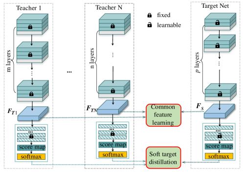
Figure 1: Illustration of the proposed heterogeneous knowledge amalgamation approach. The student and the teachers may have different network architectures. The student learns the transformed features of the teachers in a common feature space, as depicted by the common feature learning block, and meanwhile imitates the soft target predicted by the teachers, as depicted by the soft target distillation block.

In recent years, deep neural networks (DNNs) have achieved impressive success in many artificial intelligence tasks like computer vision and natural language processing. Despite the exceptional results achieved, DNNs are known to be data hungry, meaning that very large number of annotations, sometimes confidential and unavailable to the public, are required to train the models.

To alleviate the reproducing effort, many researchers have released their well-trained models online, so that the users may download and use them immediately in a plug-and-play manner. Such publicly-available trained models are, however, often of different architectures, due to rapid development of deep learning and the consequent huge number of network variants, each of which optimized for its own specific tasks or datasets.

In this paper, we investigate an ambitious deep-model reusing task, whose goal is to train a light-weight and multitalented student model, using multiple heterogeneous-architecture teacher models that specialize in different tasks. We assume we have no access to any human annotation but only well-trained teacher models, and focus on how the student model is able to amalgamate knowledge from the heterogeneous teachers.

As we impose no assumption on the teachers’ architecture being the same, it is infeasible to conduct a layer-wise knowledge amalgamation. We thus resort to an alternative approach. We project the final heterogeneous features of the teachers into a shared feature space, which is learned, and then enforce the student to imitate the transformed features of the teachers. The student model, learned in this way without accessing human annotations, amalgamates the integrated knowledge from the heterogeneous teachers and is capable of tackling all the teachers’ tasks.

The proposed approach is therefore different from and more generic than the conventional knowledge distillation (KD) Hinton et al. (2015) setup, as a student is supposed to amalgamate knowledge from multiple heterogeneous teachers in the former case yet inherit knowledge from a single teacher in the latter. It also differs from Taskonomy Zamir et al. (2018), which aims to solve multiple tasks in one system with fewer annotated data by finding transfer learning dependencies.

Specifically, we focus on knowledge amalgamation on the classification task, and test the proposed approach on a list of benchmarks of different themes. Results show that the learned student, which comes in a compact size, not only handles the complete set of tasks from all the teachers but also achieves results superior to those of the teachers in their own specialities.

Our contribution is thus a knowledge amalgamation approach tailored for training a student model, without human annotations, using heterogeneous-architecture teacher models that specialize in different tasks. This is achieved by learning a common feature space, wherein the student model imitates the transformed features of the teachers to aggregate their knowledge. Experimental results on a list of classification datasets demonstrate the learned student outperforms the teachers in their corresponding specialities.

2 Related Work

Model ensemble.

The ensemble approach combines predictions from a collection of models by weighted averaging or voting Hansen and Peter (1990); Dietterich (2000); Wang et al. (2011). It has been long observed that ensembles of multiple networks are generally much more robust and accurate than a single network. Essentially, “implicit” model ensemble usually has high efficiency during both training and testing. The typical ensemble methods include: Dropout Srivastava et al. (2014), Drop Connection Wan et al. (2013), Stochastic Depth  Huang et al. (2016), Swapout Singh et al. (2016), etc. These methods generally create an exponential number of networks with shared weights during training and then implicitly ensemble them at test time. Unlike model ensemble, our task here aims to train a single student model that performs the whole collection of tasks handled by all teachers, with no human annotations.

Knowledge distillation.

The concept of knowledge distillation is originally proposed by Hinton et al Hinton et al. (2015) for model compression Yu et al. (2017). It uses the soft targets generated by a bigger and deeper network to train a smaller and shallower network and achieves similar performance as the deeper network. Some researches Romero et al. (2015); Wang et al. (2018) extended Hinton’s work Hinton et al. (2015) by using not only the outputs but also the intermediate representations learned by the teacher as hints to train the student network. Most knowledge distillation methods Hinton et al. (2015); Romero et al. (2015); Wang et al. (2018) fall into single-teacher single-student manner, where the task of the teacher and the student is the same. Recently, Shen et al Shen et al. (2019) proposes to reuse multiple pre-trained classifiers, which focus on different classification problems, to learn a student model that handles the comprehensive task. Despite the superior effectiveness of their N-to-1 amalgamation method, they impose a strong assumption that the network architectures of the teacher are identical. The work of Ye et al Ye et al. (2019), similarly, imposes the same assumption on the network architectures. Our method, by contrast, has no such constraints and is capable of resolving the amalgamation of heterogeneous teachers.

Domain adaption.

Domain adaptation Ben-David et al. (2010); Gong et al. (2016), which belongs to transfer learning, aims at improving the testing performance on an unlabeled target domain while the model is trained on a related yet different source domain. Since there is no label available on the target domain, the core of domain adaptation is to measure and reduce the discrepancy between the distributions of these two domains. In the literature, Maximum Mean Discrepancy (MMD) Gretton et al. (2012) is a widely used criterion for measure the mismatch in different domains, which compares distributions in the Reproducing Kernel Hilbert Space (RKHS). We extend MMD to match the distribution of the common transferred features of the teachers and the student in this paper such that our method can be more robust to amalgamation of heterogeneous teachers which may be trained on datasets across domains.

3 Overview

We assume we are given $N$ teacher networks, each of which denoted by $Ti$. Our goal is to learn a single student model $S$ that amalgamates the knowledge of the teachers and masters the tasks of them, with no annotated training data. The architectures of the teacher models can be identical or different, with no specific constraints.

The overall framework of the proposed method is shown in Fig. 1. We extract the final features from the heterogeneous teachers and then project them into a learned common feature space, in which the student is expected to imitate the teachers’ features, as depicted by the common feature learning block. We also encourage the student to produce the same prediction as the teachers do, depicted by the soft target distillation block. In next section, we give more details on these blocks and our complete model.

4 Knowledge Amalgamation by Common Feature Learning

In this section, we give details of the proposed knowledge amalgamation approach. As shown in Fig. 1, the amalgamation consists of two parts: feature learning in the common space, represented by the common feature learning block, and classification score learning, represented by the soft target distillations block. In what follows, we discuss the two blocks and then give our final loss function.

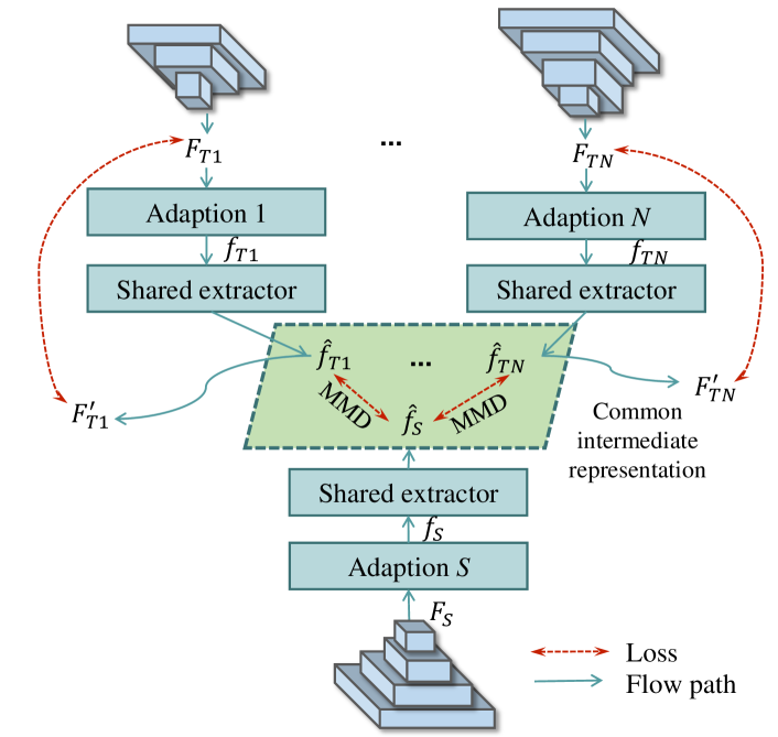
Figure 2: Illustration of the common feature learning block. Two types of losses are imposed: the first on the distances between the transformed features of the student (target net) and those of the teachers in the common space, and second on the reconstruction errors of the teachers’ features mapping back to the original space.

4.1 Common Feature Learning

The structure of the common feature learning block is shown in Fig. 2. The features of the teachers and those to be learned of the students are transformed to a common features space, via an adaption layer and a shared extractor, for which both the parameters are learned. Two loss terms are imposed: the feature ensemble loss $\mathcal{L}_{M}$ and the reconstruction loss $\mathcal{L}_{R}$. The former one encourages the features of the student to approximate those of the teachers in the common space, while the latter one ensures the transformed features can be mapped back to the original space with minimal possible errors.

4.1.1 Adaption Layer

The adaption layer is used to align the output feature dimensions of the teachers and that of the student to be the same. Thus, the teachers and the student have their individually-parameterized adaption layers. The layers are formed by convolutions with 1$\times$1 kernel Szegedy et al. (2015) that generate a predefined length of output with different input sizes. We use $F_{S}$ and $F_{Ti}$ to denote respectively the features of the student and teacher $Ti$ before being fed to the adaption layer, and use $f_{S}$ and $f_{Ti}$ to denote respectively their aligned features after passing through the adaption layer. The channel number of $f_{S}$ and $f_{Ti}$ is 256 in our implementation.

4.1.2 Shared Extractor

Once the aligned output features are derived, a straightforward approach would be to directly average the features of the teachers $f_{Ti}$ as that of the student $f_{S}$. However, due to domain discrepancy of the training data and architectural difference of the teacher networks, the roughly aligned features may still remain heterogeneous.

To this end, we introduce a small and learnable sub-network, of which the parameters are shared among the teachers and the student as shown in Fig. 2, to convert all features to a common and interactable space, which we call the common feature space. This sub-network, termed shared extractor, is a small convolution network formed by three residual block of 1$\times$1 stride. It converts $f_{Ti}$ and $f_{s}$ to the transformed features $\hat{f}_{Ti}$ and $\hat{f}_{S}$ in the common space, of which the channel number is taken to be 128 in our implementation.

4.1.3 Knowledge Amalgamation

To amalgamate knowledge from the heterogeneous teachers, we enforce the features of the student to imitate those of the teachers in the shared feature space. Specially, we adopt the Maximum Mean Discrepancy (MMD) Gretton et al. (2012), traditionally used to measure the domain mismatch in domain adaption task, in aim to align the student and teacher domains via estimated posteriors. MMD can be regarded as a distance metric for probability distributions Gretton et al. (2012). In our case, we measure the discrepancy between the output features of the student and those of the teachers.

We first focus on the discrepancy between the student and one teacher. We use $\mathcal{X}=\{\hat{f}_{T}^{i}\}_{i=0}^{C_{T}}$ to denote the set of all features of the teacher, where ${C_{T}}$ is the total number of the teacher’s features. Similar, we use $\mathcal{Y}=\{\hat{f}_{S}^{i}\}_{i=0}^{C_{S}}$ to denote all features of the student, where ${C_{S}}$ is the total number of the student’s features. An empirical approximation to the MMD distance of $\hat{f}_{T}$ and $\hat{f}_{S}$ is computed as follows:

$$\mathcal{MMD}=\|\frac{1}{C_{T}}\sum_{i=1}^{C_{T}}\phi(f_{T}^{i})-\frac{1}{C_{S}}\sum_{j=1}^{C_{S}}\phi(f_{S}^{j})\|^{2}_{2},$$ (1)

where $\phi$ is an explicit mapping function. By further expanding it using the kernel function , the MMD loss is given as:

$$\ell_{m}(\hat{f}_{T},\hat{f}_{S})= \sum_{i=1}^{C_{T}}\sum_{j=1}^{C_{T}}{\frac{\mathcal{K}(\hat{f}_{T}^{i},\hat{f}_{T}^{j})}{C_{T}^{2}}}-\sum_{i=1}^{C_{T}}\sum_{j=1}^{C_{S}}{\frac{2\mathcal{K}(\hat{f}_{T}^{i},\hat{f}_{S}^{j})}{C_{S}C_{T}}}+$$

$$+\sum_{i=1}^{C_{S}}\sum_{j=1}^{C_{S}}{\frac{\mathcal{K}(\hat{f}_{S}^{i},\hat{f}_{S}^{j})}{C_{S}^{2}}},$$ (2)

where $\mathcal{K}(\cdot,\cdot)$ is a kernel function that projects sample vectors into a higher dimensional feature space. We note that we calculated $\ell_{m}$ with normalized $\hat{f}_{T}^{j}$ and $\hat{f}_{S}^{j}$.

We then aggregate all such pairwise MMD losses between each teacher and the student, as shown in Fig. 2, and write the overall discrepancy $\mathcal{L}_{M}$ in the common space as

$$\mathcal{L}_{M}=\sum_{i=1}^{N}{\ell_{m}(\hat{f}_{Ti},\hat{f}_{S})},$$ (3)

where $N$ is the number of teachers.

To further make the learning of common feature space more robust, we add a auxiliary reconstruction loss to make sure that the transferred feature can be “mapped back”. Specially, we reconstruct the original output feature of the teacher using the transferred ones. Let $F_{Ti}^{\prime}$ denote the reconstructed feature of teacher $Ti$, the reconstruction loss $\mathcal{L}_{R}$ is defined as

$$\mathcal{L}_{R}=\sum_{i=1}^{N}\|F_{Ti}^{\prime}-F_{Ti}\|_{2},$$ (4)

4.2 Soft Target Distillation

Apart from learning the teachers’ features, the student is also expected to produce identical or similar predictions, in our case classification scores, as the teachers do. We thus also take the predictions of the teachers, by feeding unlabelled input samples, and as supervisions for training the student.

For disjoint teacher models that handle non-overlapping classes, we directly stack their score vectors, and use the concatenated score vector as the target for the student. The same strategy can in fact also be used for teachers with overlapping classes: at training time, we treat the multiple entries of the overlapping categories as different classes, yet during testing, take them to be the same category.

Let $c_{i}$ denote the function of teachers that maps the last-conv feature to the score map and $c_{s}$ denote the corresponding function of the student. The soft-target loss term $L_{C}$, which makes the response scores of the student network to approximate the predictions of the teacher, is taken as:

$$\mathcal{L}_{C}=\|c_{s}\circ F_{s}-[c_{1}\circ F_{T1},\dots,c_{N}\circ F_{TN}]\|_{2}.$$ (5)

4.3 Final Loss

We incorporate the loss terms in Eqs. (3), (4) and  (5) into our final loss function. The whole framework is trained end-to-end by optimizing the following objective:

$$\mathcal{L}=\alpha\mathcal{L}_{C}+(1-\alpha)(\mathcal{L}_{M}+\mathcal{L}_{R}),\alpha\in[0,1]$$ (6)

where $\alpha$ is a hyper-parameter to balance the three terms of the loss function. By optimizing this loss function, the student network is trained from the amalgamation of its teacher without annotations.

5 Experiment

We demonstrate the effectiveness of the proposed method on a list of benchmark, and provide implementation details, comparative results and discussions, as follows.

Classification Dataset	Categories	Images	Train/Test
Stanford Dog	120	25,580	Train/Test
Stanford Car	195	16,185	Train/Test
CUB200-2011	200	11,788	Train/Test
FGVC-Aircraft	102	10,200	Train/Test
Catech 101	101	9,146	Train/Test
Face Dataset	Identities	Images	Train/Test
CASIA	10,575	494,414	Train
MS-Celeb-1M	100K	10M	Train
CFP-FP	500	7000	Test
LFW	1,680	13,000	Test
AgeDB-30	568	16,488	Test

Table 1: Datasets for training and testing. Train/Test: usage for training or testing

5.1 Networks

In this paper, we utilize the widely used $alexnet$, $vgg$-16, and the $resnet$ He et al. (2016) family including $resnet$-18, $resnet$-34, and $resnet$-50, as our model samples. Also, we use the baseline Arcface Deng et al. (2018) network with basic cross entropy loss for the face recognition task.

5.2 Dataset and Training Details

We test the proposed method on a list of classification datasets summarized in Tab. 1.

Given a dataset, we pre-trained the teacher network against the one-hot image-level labels in advance over the dataset using the cross-entropy loss. We randomly split the categories into non-overlapping parts of equal size to train the heterogeneous-architecture teachers. The student network $S$ is trained over non-annotated training data with the score vector and prediction of the teacher networks. Once the teacher network is trained, we freeze its parameters when training the student network.

In face recognition case, we employ CASIA webface Yi et al. (2014) or MS-Celeb-1M as the training data, 1,000 identities from its overall 10K ones are used for training the teacher model. During training, we explore face verification datasets including LFW Huang et al. (2008), CFP-FP Sengupta et al. (2016), and AgeDB-30 Moschoglou et al. (2017) as the validation set.

5.3 Implement Details

We implement our method using PyTorch He et al. (2016) on a Quadro P5000 16G GPU. An Adam Kingma and Ba (2014) optimizer is utilized to train the student network. The learning rate is $e^{-4}$, while the batch size is 128 on classification datasets and 64 on face recognition ones.

5.4 Results and Analysis

We perform various experiments on different dataset to validate the proposed method. Their results and some brief analysis are presented in this subsection.

Model	Dog (%)	Catech 101(%)
T1 ($resnet$-18)	45.09	71.69
T2 ($resnet$-34)	50.65	75.36
ensemble	37.90	65.99
$resnet$-34 with GT	53.03	72.53
KD ($resnet$-34)	48.31	73.15
Ours ($resnet$-34)	53.80	73.69

Table 2: Comparison of proposed knowledge amalgamation method against others on Stanford dog and Catech 101 dataset, in terms of classification accuracy. Given two teachers trained on two class-exclusive splits of the dataset from scratch, our method outperforms not only the two teachers on their own specialized domains, but also model ensemble, the baseline KD, and even training a $resnet$-34 using ground truth data.

5.4.1 Comparison with Other Training Strategy

• Model ensemble. The score vectors of the teachers are concatenated and the input sample is classified to the class with the highest score in the concatenated vector.

• Training with GT. We train the student network from scratch with ground-truth annotations. This result is used as an reference of our unsupervised method.

• KD baseline. We apply the knowledge distillation method Hinton et al. (2015) to heterogeneous teachers extension. The score maps of the teachers are stacked and used to learn the target network.

• Homogeneous Knowledge Amalgamation. We also compare our results to the state-of-the-art homogeneous knowledge amalgamation method of Shen’s Shen et al. (2019), when applicable, since this method works only when the teachers share the same network architecture.

Model	LFW (%)	Agedb30 (%)	CFP-FP (%)
$T1$	97.43	84.72	86.20
$T2$	97.80	85.87	87.27
KD	97.15	84.97	86.87
Ours	98.10	86.93	87.73

Table 3: Comparison of the proposed knowledge amalgamation method against the teachers and KD on face recognition task. Each teacher is trained with a 3000-classes split from CASIA.

We compare the performances of the first three methods and ours in Tab. 2 and Tab. 3, since we focus here on heterogeneous teachers and thus cannot apply Shen’s method. As can be seen, the proposed methods, denoted by ours, achieves the highest accuracies. The trained student outperforms not only the two teachers, but also the $resnet$ model that trains with ground truth. The encouraging results indicate that the student indeed amalgamates the knowledge of the teachers in different domains, which potentially complement each other and eventually benefit the student’s classification.

To have a fair comparison with Shen’s method that can only handle homogeneous teachers, we adopt the same network architecture, $alexnet$, as done in Shen et al. (2019). The results are demonstrated in Tab. 4. It can be observed that our method yields an overall similar yet sometimes much better results (e.g. the case of car).

Model	Dog	CUB	Car	Aircraft
ensemble	43.5	41.4	37.8	47.1
KD	10.4	30.0	17.0	39.9
Shen et al. (2019)	45.3	42.6	40.6	49.4
Ours	44.4	43.6	45.3	47.5

Table 4: Comparing our results with homogeneous amalgamation methods on several classification datasets. Note that Dog stands for Stanford Dog, CUB for CUB200-2011, Car for Stanford Car, and Aircraft for FGVC-Aircraft.

5.4.2 More Results on Heterogeneous Teacher Architectures

As our model allows for teachers with different architectures, we test more combinations of architectures and show our results Tab. 5, where we also report the corresponding performances of KD. We test combinations of teachers with different $resnet$ and $vgg$ architectures. As can be seen, the proposed method consistently outperforms KD under all the settings. Besides, we observe that the student with more complex network architecture (deeper and wider) trends to gain significantly better performance.

Teachers	Method	Target Net (acc.%)
		$res$-18	$res$-34	$res$-50	$vgg$-16
T1 ($vgg$-16)	KD	66.4	68.6	70.5	65.6
T2 ($res$-18)	Ours	66.7	69.1	71.6	66.3
T1 ($vgg$-16)	KD	64.6	68.7	70.5	65.8
T2 ($res$-34)	Ours	66.4	69.3	71.2	66.0
T1 ($res$-18)	KD	76.2	80.2	82.0	79.2
T2 ($res$-34)	Ours	77.9	81.3	82.3	79.3
T1 ($res$-50)	KD	77.6	80.4	82.5	80.2
T2 ($res$-34)	Ours	78.5	81.6	83.8	80.8

Table 5: Comparing the results of ours and KD, using teachers of heterogeneous architectures. Results are obtained on Stanford Dog, where all the classes are split into two non-overlapping parts, each of which is used for training one teacher. Here the teachers are trained with pre-trained models on ImageNet.

5.4.3 Amalgamation with Multiple Teachers

We also test the performance of our method in multiple-teachers case. We use a target network of the $resnet$-50 backbone to amalgamate knowledge from two to four teachers, each specializes in a different classification task on different datasets. Our results are shown in Tab. 6. Again, the student is able to achieves results that are in most cases superior to those of the teachers.

Teachers	Datasets (acc. %)
	Dog	CUB	Aircraft	Car
$Ti$ arch	$resnet$-50	$resnet$-18	$resnet$-18	$resnet$-34
$Ti$ acc	87.1	75.6	73.2	82.9
2 teachers	84.3	78.9	-	-
3 teachers	83.1	77.7	79.0	-
4 teachers	82.5	77.5	78.3	84.2

Table 6: Comparative results of the teachers and the student trained with varying number of teachers. The teachers are trained for different classification tasks on distinct datasets.

5.4.4 Supervision Robustness

Here, we train the target network on two different types of data: 1) the same set of training images as the those of the teachers, which we call soft unlabeled data; 2) the totally unlabeled data that are different yet similar with the teacher’s training data, which we call hard unlabeled data. The target network is trained with the score maps and the predictions of its teachers as soft targets on both types of training data.

Specifically, given two teacher models trained on different splits of CASIA dataset, one student is trained using CASIA and therefore counted as soft unlabeled data, and the other student is trained using a totally different source of data, MS-Celeb-1M, and thus counted hard unlabeled data.

We show the results of the student trained with both the types of data in Tab. 7. As expected, the results using soft unlabeled data are better than those using hard unlabeled, but only very slightly. In fact, even using hard unlabeled data, our method outperforms KD, confirming the robustness of the proposed knowledge amalgamation.

Model	CFP-FP(%)	LFW(%)	Agedb30(%)
KD	86.87	97.15	86.87
soft unlabeled	87.73	98.12	87.73
hard unlabeled	86.36	98.12	87.00

Table 7: Comparative results of our student when trained with different types of non-annotated data, under the supervision of teachers on face recognition datasets.

5.4.5 Ablation Studies

We conduct ablation studies to investigate the contribution of the shared extractor and that of MMD described in Sec. 4.1. For shared extractor, we compare the performances by turning it on and off. For MMD, on the other hand, we replace the module with an autoencoder, which concatenates the extracted features of the teachers and encodes its channels to its half size as the target feature for the student network. We summarize the comparative results in Tab. 8, where we observe that the combination with shared extractor turned on and MMD yields the overall best performance.

Shared Ext.	AE	MMD	Dog (%)	CUB (%)
KD			80.22	75.49
	$\surd$		79.18	75.44
		$\surd$	78.75	74.25
$\surd$	$\surd$		78.92	74.44
$\surd$		$\surd$	81.34	76.34

Table 8: Results of the proposed method with 1) shared extractor turned on and off, and 2) the MMD loss replaced by an autoencoder (AE). The best result is achieved when shared extractor is turned on and MMD loss is utilized.

5.5 Visualization of the Learned Features

We also visualize in Fig. 3 the features of the teachers and those learned by the student in the common feature space. The plot is obtained by t-SNE with $\hat{f}_{Ti}$ and $\hat{f}_{S}$ of 128 dimensions. We randomly select samples of 20 classes on the two-teacher amalgamation case on Stanford dog and CUB200-2011 dataset. We zoom in three local regions for better visualization, where the first one illustrates one single class while last two illustrate multiple cluttered classes and thus are more challenging. As we can observe, the learned features of the student, in most cases of the three zoomed regions, gather around the centers of the teachers’ features, indicating the proposed approach is indeed able to amalgamate knowledge from heterogeneous teachers.

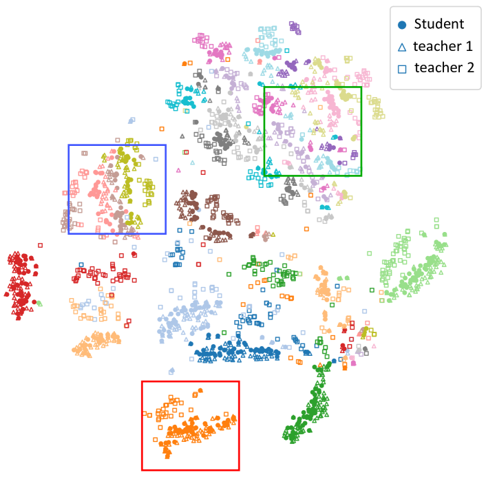
(a) t-SNE of $\hat{f}_{Ti}$ and $\hat{f}_{s}$.

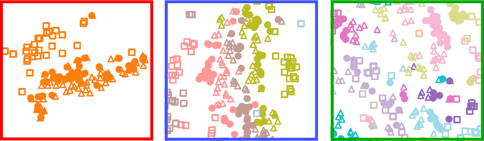
(b) Three zoomed-in regions.

Figure 3: Visualization of the features of the teachers and those learned by the student in the common feature space. The teachers are trained on Stanford dog and CUB200-2011. We randomly choose test samples of 20 classes to generate this t-SNE plot, where each color denotes a category.

6 Conclusion

We present a knowledge amalgamation approach for training a student that masters the complete set of expertise of multiple teachers, without human annotations.These teachers handle distinct tasks and are not restricted to share the same network architecture. The knowledge amalgamation is achieved by learning a common feature space, in which the student is encouraged to imitate the teachers’ features. We apply the proposed approach on several classification benchmarks, and observe that the derived student model, with a moderately compact size, achieves performance even superior to the ones of the teachers on their own task domain.

References

- Ben-David et al. [2010] Shai Ben-David, John Blitzer, Koby Crammer, Alex Kulesza, Fernando Pereira, and Jennifer Wortman Vaughan. A theory of learning from different domains. Machine learning, 79(1-2):151–175, 2010.
- Deng et al. [2018] Jiankang Deng, Jia Guo, Xue Niannan, and Stefanos Zafeiriou. Arcface: Additive angular margin loss for deep face recognition. arXiv:1801.07698, 2018.
- Dietterich [2000] Thomas G. Dietterich. Ensemble methods in machine learning. In Multiple Classifier Systems, pages 1–15, Berlin, Heidelberg, 2000. Springer.
- Gong et al. [2016] Mingming Gong, Kun Zhang, Tongliang Liu, Dacheng Tao, Clark Glymour, and Bernhard Schölkopf. Domain adaptation with conditional transferable components. In IEEE Conference on Machine Learning, 2016.
- Gretton et al. [2012] Arthur Gretton, Karsten M Borgwardt, Malte J Rasch, Bernhard Schölkopf, and Alexander Smola. A kernel two-sample test. Journal of Machine Learning Research, 13(Mar):723–773, 2012.
- Hansen and Peter [1990] Lars Kai Hansen and Salamon Peter. Neural network ensembles. IEEE Transactions on Pattern Analysis and Machine Intelligence, 12(10):993–1001, October 1990.
- He et al. [2016] Kaiming He, Xiangyu Zhang, Shaoqing Ren, and Jian Sun. Deep residual learning for image recognition. In IEEE Conference on Computer Vision and Pattern Recognition, pages 770–778, 2016.
- Hinton et al. [2015] Geoffrey Hinton, Oriol Vinyals, and Jeff Dean. Distilling the knowledge in a neural network. arXiv preprint arXiv:1503.02531, 2015.
- Huang et al. [2008] Gary B. Huang, Marwan Mattar, Tamara Berg, and Eric Learned-Miller. Labeled faces in the wild: A database forstudying face recognition in unconstrained environments. In Workshop on Faces in ’Real-Life’ Images: Detection, Alignment, and Recognition, October 2008.
- Huang et al. [2016] Gao Huang, Yu Sun, Zhuang Liu, Daniel Sedra, and Kilian Q. Weinberger. Deep networks with stochastic depth. In Proceedings of the 14th European conference on computer vision, pages 646–661, 2016.
- Kingma and Ba [2014] Diederik Kingma and Jimmy Ba. Adam: A method for stochastic optimization. arXiv preprint arXiv:1412.6980, 2014.
- Moschoglou et al. [2017] Stylianos Moschoglou, Athanasios Papaioannou, Christos Sagonas, Jiankang Deng, and Stefanos Zafeiriou. Agedb: The first manually collected, in-the-wild age database. In IEEE Conference on Computer Vision and Pattern Recognition Workshops, 2017.
- Romero et al. [2015] Adriana Romero, Nicolas Ballas, Samira Ebrahimi Kahou, Antoine Chassang, Carlo Gatta, and Yoshua Bengio. Fitnets: Hints for thin deep nets. In The International Conference on Learning Representations, 2015.
- Sengupta et al. [2016] Soumyadip Sengupta, Jun-Cheng. Chen, Carlos Castillo, Vishal M. Patel, Rama Chellappa, and David. W. Jacobs. Frontal to profile face verification in the wild. In IEEE Winter Conference on Applications of Computer Vision, pages 1–9, March 2016.
- Shen et al. [2019] Chengchao Shen, Xinchao Wang, Jie Song, Li Sun, and Mingli Song. Amalgamating knowledge towards comprehensive classification. In Proceedings of the 33th AAAI Conference on Artificial Intelligence, 2019.
- Singh et al. [2016] Saurabh Singh, Derek Hoiem, and David Forsyth. Swapout: Learning an ensemble of deep architectures. In Proceedings of the 29th Advances in Neural Information Processing Systems, pages 28–36. 2016.
- Srivastava et al. [2014] Nitish Srivastava, Geoffrey E. Hinton, Alex Krizhevsky, Ilya Sutskever, and Ruslan Salakhutdinov. Dropout: a simple way to prevent neural networks from overfitting. Journal of Machine Learning Research, 15:1929–1958, 2014.
- Szegedy et al. [2015] Christian Szegedy, Wei Liu, Yangqing Jia, Pierre Sermanet, Scott Reed, Dragomir Anguelov, Dumitru Erhan, Vincent Vanhoucke, and Andrew Rabinovich. Going deeper with convolutions. In IEEE Conference on computer vision and pattern recognition, pages 1–9, 2015.
- Wan et al. [2013] Li Wan, Matthew Zeiler, Sixin Zhang, Yann Le Cun, and Rob Fergus. Regularization of neural networks using dropconnect. In Proceedings of the 30th International Conference on Machine Learning, volume 28, pages 1058–1066, 2013.
- Wang et al. [2011] Xinchao Wang, Zhu Li, and Dacheng Tao. Subspaces indexing model on Grassmann manifold for image search. IEEE Transactions on Image Processing, 20(9):2627–2635, 2011.
- Wang et al. [2018] Hui Wang, Hanbin Zhao, Xi Li, and Xu Tan. Progressive blockwise knowledge distillation for neural network acceleration. In Proceedings of the 27th International Joint Conference on Artifical Intelligence, pages 2769–2775, 2018.
- Ye et al. [2019] Jingwen Ye, Yixin Ji, Xinchao Wang, Kairi Ou, Dapeng Tao, and Mingli Song. Student becoming the master: Knowledge amalgamation for joint scene parsing, depth estimation, and more. In IEEE Conference on Computer Vision and Pattern Recognition, 2019.
- Yi et al. [2014] Dong Yi, Zhen Lei, Shengcai Liao, and Stan Z. Li. Learning face representation from scratch. arXiv:1411.7923, 2014.
- Yu et al. [2017] Xiyu Yu, Tongliang Liu, Xinchao Wang, and Dacheng Tao. On compressing deep models by low rank and sparse decomposition. In IEEE Conference on Computer Vision and Pattern Recognition, pages 67–76, 2017.
- Zamir et al. [2018] Amir Zamir, Alexander Sax, William Shen, Leonidas Guibas, Jitendra Malik, and Silvio Savarese. Taskonomy: Disentangling task transfer learning. In IEEE Conference on Computer Vision and Pattern Recognition, pages 3712–3722, June 2018.