$l$-path vertex cover is easier than $l$-hitting set for small $l$

Abstract

In the $l$-path vertex cover problem the input is an undirected graph $G$ and an integer $k$. The goal is to decide whether there is a set of vertices $S$ of size at most $k$ such that $G-S$ does not contain a path with $l$ vertices. In this paper we give parameterized algorithms for $l$-path vertex cover for $l=5,6,7$, whose time complexities are $O^{*}(3.945^{k})$, $O^{*}(4.947^{k})$, and $O^{*}(5.951^{k})$, respectively.

Keywords

graph algorithms, parameterized complexity.

1 Introduction

For an undirected graph $G$, an $l$-path is a path in $G$ with $l$ vertices. An $l$-path vertex cover is a set of vertices $S$ such that $G-S$ does not contain an $l$-path. In the $l$-path vertex cover problem, the input is an undirected graph $G$ and an integer $k$. The goal is to decide whether there is an $l$-path vertex cover of $G$ with size at most $k$. The problem for $l=2$ is the famous vertex cover problem. For every fixed $l$, there is a simple reduction from vertex cover to $l$-path vertex cover. Therefore, $l$-path vertex cover is NP-hard for every constant $l\geq 2$.

For every fixed $l$, the $l$-path vertex cover problem is a special case of the $l$-hitting set problem. Therefore, there is a simple algorithm for $l$-path vertex cover with running time $O^{*}(l^{k})$. Better time complexities can be achieved by using the best known algorithms for $l$-hitting set. For $l=3,4,5,6$, the best algorithms for $l$-hitting set have running times of $O^{*}(2.076^{k})$, $O^{*}(3.076^{k})$, $O^{*}(4.076^{k})$, and $O^{*}(5.065^{k})$, respectively [12, 5, 4].

For specific values of $l$, it is possible to obtain algorithms for $l$-path vertex cover that are faster than the best known algorithms for $l$-hitting set. Algorithms for 3-path vertex cover were given in [10, 13, 6, 3, 14, 7], algorithms for 4-path vertex cover were given in [11, 8], and an algorithm for 5-path vertex cover was given in [2].

In this paper we give algorithms for $l$-path vertex cover for $l=5,6,7$. The time complexities of our algorithms are $O^{*}(3.945^{k})$, $O^{*}(4.947^{k})$, and $O^{*}(5.951^{k})$, respectively. See Table 1 for a comparison between our results and previous results. We note that our algorithm for $5$-path vertex cover is both faster than the algorithm of Červenỳ and Ondřej [2] and significantly simpler.

$l$	3	4	5	6	7
Old	$O^{*}(1.713^{k})$ [7]	$O^{*}(2.619^{k})$ [8]	$O^{*}(4^{k})$ [2]	$O^{*}(5.065^{k})$ [4]	$O^{*}(6.044^{k})$ [4]
New			$O^{*}(3.945^{k})$	$O^{*}(4.947^{k})$	$O^{*}(5.951^{k})$

Table 1: Comparison of old and new results for the $l$-path vertex cover problem. The old results for $l=6$ and $l=7$ are due to algorithms for $l$-hitting set.

2 The algorithm

In this section we present an algorithm for solving $l$-path vertex cover. While our algorithm is similar to the algorithm of Boral et al. [1] for the cluster vertex deletion problem, there are several important differences. In particular, the method used for computing a $v,k$-family (to be defined below) is completely different in our algorithm. For the rest of this section we consider the $l$-path vertex cover for some fixed $l$.

We first give several definitions. For set of vertices $S$ in a graph $G$, $G[S]$ is the subgraph of $G$ induced by $S$ (namely, $G[S]=(S,E\cap(S\times S))$). We also define $G-S=G[V\setminus S]$. For a path $P$ in $G$, $V(P)$ is the set of the vertices of $P$.

For a vertex $v$ in $G$, $C_{v}$ is the connected component of $G$ that contains $v$, and $G_{v}=G[C_{v}]$. A $v$-path is an $l$-path that contains $v$. A $v$-hitting set is a set of vertices $X\subseteq C_{v}\setminus\{v\}$ such that $X\cap V(P)\neq\emptyset$ for every $v$-path $P$. Denote by $\beta(G,v)$ the minimum size of a $v$-hitting set in $G$. Two $v$-paths $P,P^{\prime}$ are called intersecting if $V(P)\neq V(P^{\prime})$ and $V(P)\cap V(P^{\prime})$ contains at least one vertex other than $v$.

A $v,k$-family of a graph $G$ is a family $\mathcal{F}$ of $v$-hitting sets such that (1) Every set in $\mathcal{F}$ has size at most $k$, and (2) If $(G,k)$ is a yes instance of $l$-path vertex cover, there is a $l$-path vertex cover $S$ of $G$ of size at most $k$ such that either $v\in S$ or $A\subseteq S$ for some set $A\in\mathcal{F}$.

The following lemma will be used below to prove the correctness of the algorithm.

Lemma 1.

Let $X$ be a $v$-hitting set. There is a minimum size $l$-path vertex cover $S$ such that either $v\notin S$ or $|X\setminus S|\geq 2$.

Proof.

Let $S$ be a minimum size $l$-path vertex cover of $G$. Assume that $v\in S$ and $|X\setminus S|\leq 1$ otherwise we are done. Let $S^{\prime}=(S\setminus\{v\})\cup X$. Note that $S^{\prime}$ is also an $l$-path vertex cover of $G$ (Suppose conversely that there is an $l$-path $P$ in $G-S^{\prime}$. Since $G-S$ does not contain an $l$-path, we have that $P$ contains $v$. Namely, $P$ is a $v$-path. By definition, $X\cap V(P)\neq\emptyset$ and therefore $S^{\prime}\cap V(P)\neq\emptyset$, a contradiction). Additionally, $|S^{\prime}|\leq|S|$. Thus, $S^{\prime}$ is a minimum size $l$-path vertex cover of $G$ and $v\notin S^{\prime}$. ∎

Corollary 2.

If $\beta(G,v)=1$ then there is a minimum size $l$-path vertex cover $S$ such that $v\notin S$.

We now describe the main algorithm, which is called $\mathrm{LPVCalg}$. Algorithm $\mathrm{LPVCalg}$ is a branching algorithm. Given an instance $(G,k)$ the algorithm applies the first applicable rule from the rules below. The reduction rules of the algorithm are as follows.

R1  If $k<0$, return ‘no’.

R2  If $G$ is an empty graph, return ‘yes’.

R3  If there is a vertex $v$ such that there are no $v$-paths, return $\mathrm{LPVCalg}(G-v,k)$.

R4  If there is a vertex $v$ such that $G_{v}-v$ does not contain an $l$-path, return $\mathrm{LPVCalg}(G-C,k-1)$.

If the reduction rules above cannot be applied, the algorithm chooses an arbitrary vertex $v$. Additionally, the algorithm decides whether $\beta(G,v)$ is 1, 2, or at least 3 (this can be done in $n^{O(1)}$ time). If $\beta(G,v)=2$, the algorithm constructs a $v$-hitting set $X=\{w_{1},w_{2}\}$ of size 2. Denote by $C_{i}$ the connected component of $G_{v}-v$ that contains $w_{i}$ (note that $C_{1}$ can be equal to $C_{2}$).

Lemma 3.

If reduction rule R2 cannot be applied, $\beta(G,v)=2$, and the graphs $G[C_{1}]$ and $G[C_{2}]$ do not contain $l$-paths, then there is exactly one connected component $C_{0}$ of $G_{v}-v$ that contains an $l$-path.

Proof.

Since reduction rule R2 cannot be applied, there is at least one connected component $C_{0}$ of $G_{v}-v$ that contains an $l$-path. Suppose conversely that there is a connected component $C^{\prime}_{0}\neq C_{0}$ of $G_{v}-v$ that contains an $l$-path. Let $y_{1},\ldots,y_{l}$ be an $l$-path in $G[C_{0}]$. Let $v,x_{1},\ldots,x_{s},y_{i}$ be a shortest path in $G$ between $v$ and some vertex from $y_{1},\ldots,y_{l}$. We assume without loss of generality that $i\leq\lceil l/2\rceil$. We have that $x_{1},\ldots,x_{s},y_{i},\ldots,y_{l}$ is a path in $G[C_{0}]$ with at least $l/2$ vertices whose first vertex is adjacent to $v$. Similarly, there is a path in $G[C^{\prime}_{0}]$ with at least $l/2$ vertices whose first vertex is adjacent to $v$. Therefore, there is a $v$-path $P$ such that $V(P)\subseteq\{v\}\cup C_{0}\cup C^{\prime}_{0}$. Since $G[C_{1}]$ and $G[C_{2}]$ do not contain $l$-paths, it follows that $V(P)\cap X=\emptyset$, contradicting the fact that $X$ is a $v$-hitting set. ∎

The algorithm now tries to apply the following reduction rules.

R5  If $\beta(G,v)=2$, the graphs $G[C_{1}]$ and $G[C_{2}]$ do not contain $l$-paths, and there is a $v$-path that does not contain a vertex from $C_{0}$, return $\mathrm{LPVCalg}(G-v,k-1)$.

Rule R3 is safe since there is a minimum size $l$-path vertex cover that contains $v$: If $S$ is a minimum size $l$-path vertex cover that does not contain $v$, then $S$ must contain a vertex $x\in V(P)\setminus\{v\}$, where $P$ is a $v$-path that does not contain a vertex from $C_{0}$. By Lemma 3, the connected component of $G_{v}-v$ that contains $x$ does not contain an $l$-path. Therefore, the set $S^{\prime}=(S\setminus\{x\})\cup\{v\}$ is an $l$-path vertex cover of $G$. Since $|S^{\prime}|=|S|$, we obtain that $S^{\prime}$ is a minimum size $l$-path vertex cover that contain $v$.

R6  If $\beta(G,v)=2$ and the graphs $G[C_{1}]$ and $G[C_{2}]$ do not contain $l$-paths, return $\mathrm{LPVCalg}(G^{\prime},k)$ where the graph $G$ is obtained from $G$ as follows. Let $r$ be the maximum length of a path that starts at $v$ in $G_{v}-C_{0}$. Delete the vertices of $C_{v}\setminus(C_{0}\cup\{v\})$ from $G$, add $r$ new vertices to the graph, construct an $r$-path on the new vertices, and add an edge between the $v$ and the first vertex in the $r$-path.

The safeness of Rule R3 also follows from Lemma 3. When the reduction rules above cannot be applied, the algorithm computes a $v,k$-family $\mathcal{F}_{v,k}$ (we will describe below how to compute $\mathcal{F}_{v,k}$). It then applies one of the following branching rules, depending on $\beta(G,v)$.

B1  If $\beta(G,v)=1$, branch on every set in $\mathcal{F}_{v,k}$.

The safeness of Rule 3 follows from Corollary 2.

B2  If $\beta(G,v)=2$, let $i$ be an index such that $G[C_{i}]$ contains an $l$-path. Construct a $(w_{i},k-1)$-family $\mathcal{F}_{w_{i},k-1}^{G-v}$ for the graph $G-v$. Branch on every set in $\mathcal{F}_{v,k}$ and on $\{v\}\cup S$ for every $S\in\mathcal{F}_{w_{i},k-1}^{G-v}$.

Note that since Rule R3 cannot be applied, the index $i$ exists. By Lemma 1 there is a minimum size $l$-path vertex cover $S$ such that either $v\notin S$ or $w_{i}\notin S$. Therefore Rule B3 is safe.

B3  If $\beta(G,v)\geq 3$ branch on $\{v\}$ and on every set in $\mathcal{F}_{v,k}$.

We now describe an algorithm, called $\mathrm{Falg}$, for constructing a $v,k$-family for $G$. We will show in Section 4 that if there are no two intersecting $v$-paths then $G$ has a simple structure and thus finding a $v,k$-family for $G$ can be done in polynomial time. Moreover, the $v,k$-family in this case consists of a single set.

Algorithm $\mathrm{Falg}$ consists of the following reduction and branching rules.

FR1  If $k<0$, return $\emptyset$.

FR2  If there are no $v$-paths in $G$, return $\{\emptyset\}$.

FR3  If there are no intersecting $v$-paths, compute a $v,k$-family for $G$ and return it.

FB1  Otherwise, let $P$ and $P^{\prime}$ be intersecting $v$-paths. Perform the following steps. $L\leftarrow\emptyset$.
$a\in(V(P)\cap V(P^{\prime}))\setminus\{v\}$ $X\in\mathrm{Falg}(G-a,k-1)$ Add $X\cup\{a\}$ to $L$.
$a\in V(P)\setminus(V(P^{\prime})\cup\{v\})$ and $a^{\prime}\in V(P^{\prime})\setminus(V(P)\cup\{v\})$ $X\in\mathrm{Falg}(G-\{a,a^{\prime}\},k-2)$ Add $X\cup\{a,a^{\prime}\}$ to $L$.
$L$.

3 Analysis

In this section we analyze the running time of algorithm $\mathrm{LPVCalg}$. The analysis is similar to the analysis of the algorithm of Boral et al. [1] (see also [9]).

Let $A$ be some parameterize algorithm on graphs. The run of algorithm $A$ on an input $(G,k)$ can be represented by a recursion tree, denoted $T_{A}(G,k)$, as follows. The root $r$ of the tree corresponds to the call $A(G,k)$. If the algorithm terminates in this call, the root $r$ is a leaf. Otherwise, suppose that the algorithm is called recursively on the instances $(G_{1},k-a_{1}),\ldots,(G_{t},k-a_{t})$. In this case, the root $r$ has $t$ children. The $i$-th child of $r$ is the root of the tree $T_{A}(G_{i},k-a_{i})$. The edge between $r$ and its $i$-th child is labeled by $a_{i}$. See Figure 1(a) for an example.

We define the weighted depth of a node $x$ in $T_{A}(G,k)$ to be the sum of the labels of the edges on the path from the root to $x$. For an internal node $x$ in $T_{A}(G,k)$ define the branching vector of $x$ to be a vector containing the labels of the edges between $x$ and its children. The branching number of a vector $(a_{1},\ldots,a_{t})$ (where $t\geq 2$) is the largest root of $P(x)=1-\sum_{i=1}^{t}x^{-a_{i}}$. The branching number of a node $x$ in $T_{A}(G,k)$ is the branching number of the branching vector of $x$. The running time of algorithm $A$ can be bounded by bounding the number of leaves in $T_{A}(G,k)$. The number of leaves in $T_{A}(G,k)$ is $O(c^{k})$, where $c$ is the maximum branching number of a node in the tree.

From the previous paragraph, we can bound the number of leaves in $T_{A}(G,k)$ by giving an upper bound on the branching number of a node in $T_{A}(G,k)$. In some cases, there may be few nodes in $T_{A}(G,k)$ with large branching numbers. One can handle this case by modifying the tree $T_{A}(G,k)$ by contracting some of its edges. If $x$ is a node in $T_{A}(G,k)$ and $y$ is a child of $x$ which is an internal node, contracting the edge $(x,y)$ means deleting the node $y$ and replacing every edge $(y,z)$ between $y$ and a child $z$ of $y$ with an edge $(x,z)$. The label of $(x,z)$ is equal to the label of $(x,y)$ plus the label of $(y,z)$. See Figure 1(b). Note that after edge contractions, the number of leaves in the contracted tree is equal to the number of leaves in $T_{A}(G,k)$. However, the maximum branching number of a node in the contracted tree may be smaller than the maximum branching number of a node in $T_{A}(G,k)$.

For an integer $\alpha$, we define the top recursion tree $T^{\alpha}_{A}(G,k)$ to be the tree obtained by taking the subtree of $T_{A}(G,k)$ induced by the nodes with weighted depth less than $\alpha$ and their children. See Figure 1(c) for an example.

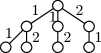
(a) $T_{A}(G,k)$

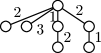
(b) Contraction

(c) $T^{2}_{A}(G,k)$

Figure 1: Figure (a) shows a recursion tree $T_{A}(G,k)$. In this example, the call $A(G,k)$ makes three recursive calls: $A(G_{1},k-1)$, $A(G_{2},k-1)$, and $A(G_{3},k-2)$. Figure (b) shows the tree $T_{A}(G,k)$ after contracting the edge between the root and its leftmost child. The top recursion tree $T^{2}_{A}(G,k)$ is shown in Figure (c).

When we consider the recursion tree $T_{\mathrm{Falg}}(G,k)$ of algorithm $\mathrm{Falg}$, we assume that if in the recursive call on an instance $(G^{\prime},k^{\prime})$ the algorithm applies Rule FR3 then the node $x$ in $T_{\mathrm{Falg}}(G,k)$ that corresponds to this call has a single child $x^{\prime}$ (which is a leaf) and the label of the edge $(x,x^{\prime})$ is the cardinality of the single set in the computed family.

To analyze the algorithm we define a tree $T(G,k)$ that represents the recursive calls to both $\mathrm{LPVCalg}$ and $\mathrm{Falg}$. Consider a node $x$ in $T_{\mathrm{LPVCalg}}(G,k)$, corresponding to a recursive call $\mathrm{LPVCalg}(G^{\prime},k^{\prime})$. Suppose that in the recursive call $\mathrm{LPVCalg}(G^{\prime},k^{\prime})$, the algorithm applies Rule B3. Recall that in this case, the algorithm branches on $\{v\}$ and on every set in $\mathcal{F}_{v,k^{\prime}}$. Denote $\mathcal{F}_{v,k^{\prime}}=\{X_{1},\ldots,X_{t}\}$. In the tree $T_{\mathrm{LPVCalg}}(G,k)$, $x$ has $t+1$ children $y,x_{1},\ldots,x_{t}$ (the child $y$ corresponds to the recursive call on $(G^{\prime}-v,k^{\prime}-1)$, and a child $x_{i}$ corresponds to the recursive call on $(G^{\prime}-X_{i},k^{\prime}-|X_{i}|)$). The label of the edge $(x,y)$ is $1$, and the label of an edge $(x,x_{i})$ is $|X_{i}|$. The tree $T(G,k)$ also contains the nodes $x,y,x_{1},\ldots,x_{t}$. In $T(G,k)$, $x$ has two children $y$ and $x^{\prime}$, where $x^{\prime}$ is a new node. The labels of the edges $(x,y)$ and $(x,x^{\prime})$ are $1$ and $0$, respectively. The node $x^{\prime}$ is the root of a copy of the tree $T_{\mathrm{Falg}}(G^{\prime},k^{\prime})$ and the nodes $x_{1},\ldots,x_{t}$ are the leaves of this tree. Note that the label of an edge $(x,x_{i})$ in the tree $T_{\mathrm{LPVCalg}}(G,k)$ is equal to the sum of the labels of the edges on the path from $x$ to $x_{i}$ in the tree $T(G,k)$.

Similarly, if in the recursive call $\mathrm{LPVCalg}(G^{\prime},k^{\prime})$ that corresponds to $x$ the algorithm applies Rule B3, then the algorithm branches on every set in $\mathcal{F}_{v,k^{\prime}}$ and on $\{v\}\cup S$ for every $S\in\mathcal{F}_{w_{i},k^{\prime}-1}^{G-v}$. Denote $\mathcal{F}_{v,k^{\prime}}=\{X_{1},\ldots,X_{t}\}$ and $\mathcal{F}_{w_{i},k^{\prime}-1}^{G-v}=\{Y_{1},\ldots,Y_{s}\}$. In the tree $T_{\mathrm{LPVCalg}}(G,k)$, $x$ has $s+t$ children $y_{1},\ldots,y_{s},x_{1},\ldots,x_{t}$. The label of an edge $(x,x_{i})$ is $|X_{i}|$, and the label of an edge $(x,y_{i})$ is $1+|Y_{i}|$. In the tree $T(G,k)$, $x$ has two children $y^{\prime}$ and $x^{\prime}$. The labels of the edges $(x,y^{\prime})$ and $(x,x^{\prime})$ are $1$ and $0$, respectively. The node $x^{\prime}$ is the root of a copy of the tree $T_{\mathrm{Falg}}(G^{\prime},k^{\prime})$, and $x_{1},\ldots,x_{t}$ are the leaves of this tree. The node $y^{\prime}$ is the root of a copy of the tree $T_{\mathrm{Falg}}(G^{\prime}-v,k^{\prime}-1)$, and $y_{1},\ldots,y_{s}$ are the leaves of this tree.

Finally, suppose that in the recursive call $\mathrm{LPVCalg}(G^{\prime},k^{\prime})$ that corresponds to $x$, the algorithm applies Rule B3. In this case, the algorithm branches on every set in $\mathcal{F}_{v,k^{\prime}}$. In the tree $T_{\mathrm{LPVCalg}}(G,k)$, $x$ has $t=|\mathcal{F}_{v,k^{\prime}}|$ children $x_{1},\ldots,x_{t}$. In $T(G,k)$, the node $x$ is the root of a copy of the tree $T_{\mathrm{Falg}}(H^{\prime},k^{\prime})$, and $x_{1},\ldots,x_{t}$ are the leaves of this tree.

Our goal is to analyze the number of leaves in $T(G,k)$. For this purpose, we perform edge contractions on $T(G,k)$ to obtain a tree $T_{\mathrm{C}}(G,k)$. Consider a node $x$ in $T(G,k)$ that corresponds to a recursive call $\mathrm{LPVCalg}(G^{\prime},k^{\prime})$. Suppose that in the recursive call $\mathrm{LPVCalg}(G^{\prime},k^{\prime})$, the algorithm applies Rule B3. Using the same notations as in the paragraphs above, we contract the following edges:

1. The edge $(x,x^{\prime})$.

2. The edges of the copy of $T_{\mathrm{Falg}}(G^{\prime},k^{\prime})$ whose endpoints correspond to internal nodes in the tree $T^{3}_{\mathrm{Falg}}(G^{\prime},k^{\prime})$. In other words, the two endpoints of such edges have weighted depths less than $3$ in the copy of $T_{\mathrm{Falg}}(G^{\prime},k^{\prime})$.

If in the recursive call $\mathrm{LPVCalg}(G^{\prime},k^{\prime})$ the algorithm applies Rule B3, we contract the following edges.

1. The edges $(x,y^{\prime})$ and $(x,x^{\prime})$.

2. The edges of the copy of $T_{\mathrm{Falg}}(G^{\prime},k^{\prime})$ whose endpoints correspond to internal nodes in the tree $T^{2}_{\mathrm{Falg}}(G^{\prime},k^{\prime})$.

If in the recursive call $\mathrm{LPVCalg}(G^{\prime},k^{\prime})$ the algorithm applies Rule B3, we do not contract edges.

The nodes in $T(G,k)$ and $T_{\mathrm{C}}(G,k)$ that correspond to nodes in $T_{\mathrm{LPVCalg}}(G,k)$ are called primary nodes, and the remaining nodes are secondary nodes.

If $x$ is a secondary node of $T(G,k)$ with more than one child, the branching vector of $x$ is of the form $V_{s}=(1,\ldots,1,2,\ldots,2)$, where the value 1 appears $s$ times for some $s\leq l-2$ and the value 2 appears $(l-1-s)^{2}$ times. The vector among $V_{1},\ldots,V_{l-2}$ with largest branching number is $V_{1}$. For $l=4$, for example, $V_{1}=(1,2,2,2,2)$ and the branching number of $V_{1}$ is less than 2.562. Therefore the branching number of all the secondary nodes in $T_{\mathrm{C}}(G,k)$ and all the primary nodes that correspond to recursive calls in which Rule B3 is applied have branching numbers less than 2.562.

We now bound the branching numbers of the remaining primary nodes of $T_{\mathrm{C}}(G,k)$. Let $x$ be a primary node and suppose that in the corresponding recursive call $\mathrm{LPVCalg}(G^{\prime},k^{\prime})$ the algorithm applies Rule B3. Using the same notations as in the paragraphs above, the branching vector of $x$ is $(1,c_{1},\ldots,c_{t})$, where $(c_{1},\ldots,c_{t})$ are the weighted depths of the leaves of the top recursion tree $T^{3}_{\mathrm{Falg}}(G^{\prime},k^{\prime})$. The top recursion tree that gives the worst branching number is the tree in which every internal node has branching vector $V_{1}$. See Figure 2. For $l=4$, the branching vector of $x$ in this case is

$$(1,3,4,4,4,4,3,3,3,3,3,4,4,4,4,3,4,4,4,4,3,4,4,4,4,3,4,4,4,4)$$

and the branching number is less than 2.897.

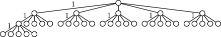
Figure 2: The worst top recursion tree for $l=4$. The branching vector of every internal node is $(1,2,2,2,2)$. Edges whose labels are not shown have label 2.

If in the recursive call $\mathrm{LPVCalg}(G^{\prime},k^{\prime})$ the algorithm applies Rule B3 then the branching vector of $x$ has the form $(1+a,c_{1},\ldots,c_{t})$ for $a\geq 1$, or the form $(2,\ldots,2,3,\ldots,3,c_{1},\ldots,c_{t})$, where where $(c_{1},\ldots,c_{t})$ are the weighted depths of the leaves of the top recursion tree $T^{2}_{\mathrm{Falg}}(G^{\prime},k^{\prime})$, and in the second form the value 2 appears $s$ times for some $s\leq l-2$ and the value 3 appears $(l-1-s)^{2}$ times. The worst case is when the branching vector is of the form $(2,3,\ldots,3,c_{1},\ldots,c_{t})$, where the value 3 appears $(l-2)^{2}$ times. Additionally, the top recursion tree that gives the worst branching number is the tree in which every internal node has branching vector $V_{1}$. For $l=4$, the branching vector of $x$ in this case is

$$(2,3,3,3,3,2,3,3,3,3,2,2,2,2)$$

and the branching number is less than 2.952.

It follows that for $l=4$, all nodes of $T_{\mathrm{C}}(G,k)$ have branching numbers less than 2.952. Therefore, the time complexity of the algorithm for $l=4$ is $O^{*}(2.952^{k})$. Similarly, for $l=5,6,7$, the time complexities of the algorithm are $O^{*}(3.945^{k})$, $O^{*}(4.947^{k})$, and $O^{*}(5.951^{k})$, respectively.

4 Graphs with no intersecting $v$-paths

In this section we show how to compute a $v,k$-family in a graph $G$ that does not contain two intersecting $v$-paths. We will show that when $l\leq 7$ the graph $G$ has a simple structure, and we will use this fact to obtain an algorithm for computing a $v,k$-family.

A $v$-path $P=x^{\prime}_{1},\ldots,x^{\prime}_{p},v,\allowbreak x_{1},\ldots,x_{l-1-p}$ (where $p$ can be 0) is called canonical if $p\leq\lfloor(l-1)/2\rfloor$ and there is no path $P^{\prime}=y^{\prime}_{1},\ldots,y^{\prime}_{q},v,y_{1},\ldots,y_{l-1-q}$ such that $V(P^{\prime})=V(P)$ and $q<p$.

Lemma 4.

Let $G$ be a graph that does not contain two intersecting $v$-paths. Then, all $v$-paths in $G$ have the same vertex set.

Proof.

Suppose conversely that $P$ and $P^{\prime}$ are canonical $v$-paths such that $V(P)\neq V(P^{\prime})$. Since $P$ and $P^{\prime}$ do not intersect, $V(P)\cap V(P^{\prime})=\{v\}$. Denote $P=x^{\prime}_{1},\ldots,x^{\prime}_{p},v,\allowbreak x_{1},\ldots,x_{l-1-p}$ and $P^{\prime}=y^{\prime}_{1},\ldots,y^{\prime}_{q},v,y_{1},\ldots,y_{l-1-q}$. The path $P^{\prime\prime}=x_{l-1-p},\ldots,x_{1},v,y_{1},\ldots,y_{l-1-q}$ is a path with at least $l$ vertices. Thus, the first $l$ vertices of $P^{\prime\prime}$ is a $v$-path that intersects $P$, a contradiction. ∎

For the rest of this section, assume that $G$ is a graph that does not contain two intersecting $v$-paths. We also assume that $P=x^{\prime}_{1},\ldots,x^{\prime}_{p},v,x_{1},\ldots,x_{l-1-p}$ is a cannonical $v$-path in $G$.

4.1 $l\leq 6$

We now consider the case $l\leq 6$. We will discuss the case $l=7$ in the next subsection.

Lemma 5.

If $l\leq 6$, for every connected component $C$ of $G_{v}-V(P)$ there is exactly one vertex in $V(P)$ that has neighbors in $C$.

Proof.

Denote $x_{0}=v$. Note that $l\geq 6$ implies that $p\leq 2$. Therefore, a vertex $x^{\prime}_{i}$ does not have neighbors in $V(G)\setminus V(P)$ (otherwise, if $x^{\prime}_{i}$ is adjacent to $y\in V(G)\setminus V(P)$, the path $y,x^{\prime}_{i},\ldots,x^{\prime}_{p},v,x_{1},\ldots,x_{l-1-p}$ is a path with at least $l$ vertices, and therefore there is a $v$-path that intersects $P$, a contradiction).

Suppose conversely that there is a connected component $C$ of $G_{v}-V(P)$ such that there are at least two vertices in $V(P)$ that have neighbors in $C$. By the above, these vertices are from $\{x_{0},\ldots,x_{l-1-p}\}$. Suppose that $x_{i}$ and $x_{j}$ have neighbors in $C$, where $i<j$. Since $C$ is a connected component of $G_{v}-V(P)$, there is a path $x_{i},y_{1},\ldots,y_{s},x_{j}$ in $G$ such that $y_{1},\ldots,y_{s}\in C$. If $s>j-i-2$ then the path $x^{\prime}_{1},\ldots,x^{\prime}_{p},v,x_{1},\ldots,x_{i},y_{1},\ldots,y_{s},x_{j},\ldots,x_{l-1-p}$ has $l-(j-i-1)+s\geq l$ vertices, and therefore there is a $v$-path that intersects $P$, a contradiction. Therefore, $s\leq j-i-2$. If either $i>0$ or $p>0$, the path $x^{\prime}_{1},\ldots,x^{\prime}_{p},v,x_{1},\ldots,x_{i},y_{1},\ldots,y_{s},x_{j},\ldots,x_{i+1}$ has $p+1+j+s\geq p+1+(s+i+2)+s\geq p+i+5\geq 6\geq l$ vertices, and therefore there is a $v$-path that intersects $P$, a contradiction. The remaining case is when $i=0$ and $p=0$. In this case, $y_{1},v,x_{1},\ldots,x_{l-2}$ is a $v$-path that intersects $P$, a contradiction. ∎

Lemma 6.

If $l\leq 6$ and $C$ is a connected component of $G_{v}-V(P)$ that contains an $l$-path then the unique vertex in $V(P)$ that has neighbors in $C$ is $x_{l-1-p}$.

Proof.

Let $x$ be the unique vertex in $V(P)$ that has neighbors in $C$. Let $P^{\prime}=y_{1},\ldots,y_{l}$ be an $l$-path in $C$. Let $y_{q}$ be the vertex in $V(P^{\prime})$ that is closest to $x$, and suppose without loss of generality that $q\leq\lceil l/2\rceil$. Let $x,z_{1},\ldots,z_{s},y_{q}$ be the shortest path from $x$ to $y_{q}$ ($s$ can be 0).

We now show that if $i<l-1-p$ then $x\neq x_{i}$. Suppose conversely that $x=x_{i}$. The path $v,x_{1},\ldots,x_{i},z_{1},\ldots,z_{s},y_{q},\ldots,y_{l}$ has at least $2+\lceil(l+1)/2\rceil\geq l$ vertices (since $l\leq 6$), and therefore there is a $v$-path that intersects $P$, a contradiction. Therefore, $x\neq x_{i}$ for every $i<l-1-p$. Similarly, $x\notin\{x^{\prime}_{1},\ldots,x^{\prime}_{p},v\}$. ∎

For a $v$-hitting set $X$, let $\alpha(x)$ be the maximum integer $q$ such that there is a $q$-path in $G-X$ whose first vertex is $x_{l-1-p}$ and its second vertex is $x_{l-2-p}$. If $x_{l-1-p}\in X$ then define $\alpha(X)=0$ and if $x_{l-1-p}\notin X$ and $x_{l-2-p}\in X$ then define $\alpha(X)=1$. A minimum size $v$-hitting set $X$ is called optimal if $\alpha(X)\leq\alpha(Y)$ for every minimum size $v$-hitting set $Y$.

Lemma 7.

If $l\leq 6$, $X$ is an optimal $v$-hitting set, and $|X|\leq k$ then $\mathcal{F}=\{X\}$ is a $v,k$-family.

Proof.

Suppose that $S$ is an $l$-path vertex cover of $G$ of size at most $k$. If $v\in S$ we are done. Suppose that $v\notin S$. Let $S_{0}$ be the set of all vertices in $S$ that are contained in $v$-paths of $G$. Since $X$ is a minimum size $v$-hitting set, $|S_{0}|\geq|X|$. By Lemma 6 and the optimality of $X$, if $|S_{0}|=|X|$ then $(S\setminus S_{0})\cup X$ is an $l$-path vertex cover of $G$ of size at most $k$. Otherwise we have $|S_{0}|>|X|$ and therefore $(S\setminus S_{0})\cup X\cup\{x_{l-1-p}\}$ is an $l$-path vertex cover of $G$ of size at most $k$. ∎

Lemma 8.

If $l\leq 6$, there is an optimal $v$-hitting set $X$ such that $X\subseteq V(P)$.

Proof.

Let $X$ be an optimal $v$-hitting set $X$. If there is a vertex $x\in X\setminus V(P)$, let $C$ be the connected component of $G_{v}-V(P)$ containing $x$ (note that $x\in C_{v}$ due to the minimality of $X$). Let $y$ be the unique vertex in $V(P)$ that has neighbors in $C$. The set $X^{\prime}=(X\setminus\{x\})\cup\{y\}$ is also a $v$-hitting set. Additionally, $|X^{\prime}|=|X|$ and $\alpha(X^{\prime})\leq\alpha(X)$. By repeating this process we obtain an optimal $v$-hitting set that is contained in $V(P)$. ∎

We now describe how to construct a $v,k$-family of a graph $G$ that does not contain intersecting $v$-sets (assuming that $l\leq 6$). By enumerating all subsets of $V(P)$, we can find an optimal $v$-hitting set $X\subseteq V(P)$. By Lemma 7, the family $\mathcal{F}=\{X\}$ is a $v,k$-family of $G$.

4.2 $l=7$

We now describe the differences between the case $l=7$ and the case $l\leq 6$.

First, in contrast to Lemma 6, it is possible that there is connected component $C$ of $G-V(P)$ such that $C$ contains an $l$-path and there is a vertex $x\in V(P)\setminus\{x_{l-1-p}\}$ that is adjacent to a vertex in $C$. It can be shown that in this case, $x=x_{1}$. Additionally, $x_{1}$ is adjacent to a single vertex $y$ in $C$, and every $l$-path in $C$ must contain $y$. It follows that if $S$ is an $l$-path vertex cover of $G$ and $y\notin S$ then $(S\setminus C)\cup\{y\}$ is also an $l$-path vertex cover of $G$.

In contrast to Lemma 5, it is possible that there is a connected component $C$ of $G_{v}-V(P)$ such that there are two vertices in $V(P)$ that have neighbors in $C$. It is easy to show that in this case the vertices in $V(P)$ that have neighbors in $C$ are $x_{1}$ and $x_{4}$. Additionally, $|C|=1$ (otherwise there is a $v$-path $v,x_{1},\ldots,x_{4},y,y^{\prime}$, where $y,y^{\prime}\in C$, and this $v$-path intersects $P$, a contradiction). We call such a connected component an $x_{1}/x_{4}$-component. Note that there can be several $x_{1}/x_{4}$-components.

We now claim that Lemma 8 is also true when $l=7$. To show that we need to consider the case when there are $x_{1}/x_{4}$-components. Suppose that $C=\{y\}$ is an $x_{1}/x_{4}$-component. We claim that every 7-path that contains $y$ also contains $x_{4}$. Suppose conversely that $P^{\prime}$ is a 7-path that contains $y$ and does not contain $x_{4}$. Then $P^{\prime}$ must be of the form $y,x_{1},\ldots,x_{i},y_{1},\ldots,y_{6-i}$ where $i\leq 3$ and $y_{1},\ldots,y_{6-i}$ are vertices in some connected component of $G_{v}-V(P)$. The path $v,x_{1},\ldots,x_{i},y_{1},\ldots,y_{6-i}$ is a $v$-path that intersects $v$, a contradiction. Therefore, the claim is true. From the claim we have that if $X$ is an optimal $v$-hitting set then $X^{\prime}=(S\setminus\{y\})\cup\{x_{4}\}$ is also an optimal $v$-hitting set. Therefore, Lemma 8 is also true when $l=7$.

From the above discussion, we can construct a $v,k$-family of $G$ using the same algorithm described above for the case $l\leq 6$.

5 Concluding remarks

We have shown algorithms for $l$-path vertex cover for $l=5,6,7$ that are faster than previous algorithms. It may be possible to use our approach for $l=8$ or other small values of $l$ by giving a more involved case analysis of graphs that do not have intersecting $v$-paths. An interesting open question is whether $l$-path vertex cover can be solved in $O^{*}((l-1-\epsilon)^{k})$ time for every value of $l$.

References

- [1] Anudhyan Boral, Marek Cygan, Tomasz Kociumaka, and Marcin Pilipczuk. A fast branching algorithm for cluster vertex deletion. Theory of Computing Systems, 58(2):357–376, 2016.
- [2] Radovan Červenỳ and Ondřej Suchỳ. Faster FPT algorithm for 5-path vertex cover. In Proc. 44th Symposium on Mathematical Foundations of Computer Science (MFCS), 2019.
- [3] Maw-Shang Chang, Li-Hsuan Chen, Ling-Ju Hung, Peter Rossmanith, and Ping-Chen Su. Fixed-parameter algorithms for vertex cover . Discrete Optimization, 19:12–22, 2016.
- [4] Henning Fernau. Parameterized algorithms for hitting set: The weighted case. In Italian Conference on Algorithms and Complexity (CIAC), pages 332–343, 2006.
- [5] Fedor V Fomin, Serge Gaspers, Dieter Kratsch, Mathieu Liedloff, and Saket Saurabh. Iterative compression and exact algorithms. Theoretical Computer Science, 411(7-9):1045–1053, 2010.
- [6] Ján Katrenič. A faster FPT algorithm for 3-path vertex cover. Information Processing Letters, 116(4):273–278, 2016.
- [7] D. Tsur. Parameterized algorithm for 3-path vertex cover. Theoretical Computer Science, 783:1–8, 2019.
- [8] D. Tsur. An algorithm for 4-path vertex cover. arXiv preprint arXiv:1811.03592, 2018.
- [9] D. Tsur. Faster parameterized algorithm for cluster vertex deletion. arXiv preprint arXiv:1901.07609, 2019.
- [10] Jianhua Tu. A fixed-parameter algorithm for the vertex cover problem. Information Processing Letters, 115(2):96–99, 2015.
- [11] Jianhua Tu and Zemin Jin. An FPT algorithm for the vertex cover problem. Discrete Applied Mathematics, 200:186–190, 2016.
- [12] Magnus Wahlström. Algorithms, measures and upper bounds for satisfiability and related problems. PhD thesis, Department of Computer and Information Science, Linköpings universitet, 2007.
- [13] Bang Ye Wu. A measure and conquer approach for the parameterized bounded degree-one vertex deletion. In Proc. 21st International Computing and Combinatorics Conference (COCOON), pages 469–480, 2015.
- [14] Mingyu Xiao and Shaowei Kou. Kernelization and parameterized algorithms for 3-path vertex cover. In Proc. 14th International Conference on Theory and Applications of Models of Computation (TAMC), pages 654–668, 2017.