Keep soft robots soft - a data-driven based trade-off between feed-forward and feedback control

Abstract

Tracking control for soft robots is challenging due to uncertainties in the system model and environment. Using high feedback gains to overcome this issue results in an increasing stiffness that clearly destroys the inherent safety property of soft robots. However, accurate models for feed-forward control are often difficult to obtain. In this article, we employ Gaussian Process regression to obtain a data-driven model that is used for the feed-forward compensation of unknown dynamics. The model fidelity is used to adapt the feed-forward and feedback part allowing low feedback gains in regions of high model confidence.

I Introduction

Soft robots represent one significant evolution of robotic systems, since they are designed to embody safe and natural behaviors [5]. The control of the robots is often challenging due to complex physical structures based on the soft materials. A common approach is to derive a simple, dynamic model from first order physics and increase the feedback gains to compensate the uncertainties until a desired tracking performance is achieved [15]. However, high gain control is undesirable since this results in an increased stiffness that destroys the inherent safety properties [5]; deriving a more accurate model of the system is often difficult if not impossible [1].
To overcome this issue, data-driven techniques deliver promising results in modeling and control of soft robot dynamics [14, 10, 4]. The accurate model based on data-driven techniques allows a more precise feed-forward control such that high feedback gains are needless. However, it is often difficult to decide if the quality of the model is good enough to rely on feed-forward control only or if feedback control is required to ensure the tracking performance.
Gaussian Process regression (GPR) is a supervised learning technique which provides not only a mean function but also a predicted variance, and therefore a measure of the model fidelity based on the distance to the training data. It requires only a minimum of prior knowledge, generalizes well even for small training data sets and has a precise trade-off between fitting the data and smoothing [13].
In this article, we present a GPR based control law for soft robots with automatic trade-off between feed-forward and feedback control. For this purpose, a GP learns the unknown system dynamics from training data. The proposed control law uses the mean of the GPR to compensate the unknown dynamics in a feed-forward manner and the model fidelity to adapt the influence of the feedback control part. As result, the the robot is softer in regions with training data.

II Methodology

We focus on the class of pneumatic- or tendon-actuated, worm-like robots. For the modeling, the robot is virtually separated into $n_{s}\gg 1$ rigid sections with constant curvature, see e.g. [12]. Each section consists of $n_{a}$ actuators, e.g. the number of muscles. Falkenhahn et al. [7], Della Santina et al. [6] develop for such class of robots an approximated dynamical model given by

$${\boldsymbol{\tau}}({\boldsymbol{q}},{\boldsymbol{p}})=M({\boldsymbol{q}})\ddot{{\boldsymbol{q}}}+C(\dot{{\boldsymbol{q}}},{\boldsymbol{q}})\dot{{\boldsymbol{q}}}+N(\dot{{\boldsymbol{q}}},{\boldsymbol{q}}),\,{\boldsymbol{y}}={\boldsymbol{g}}({\boldsymbol{q}}),$$ (1)

where ${\boldsymbol{q}}\in\mathbb{R}^{n},n=n_{s}n_{a}$ is the generalized vector of positions and ${\boldsymbol{y}}\in\mathbb{R}^{m}$ the output of the system defined by the sensors used, e.g. a vision based system [8]. In addition, there are the positive definite mass matrix $M({\boldsymbol{q}})\in\mathbb{R}^{n\times n}$, the Coriolis matrix $C(\dot{{\boldsymbol{q}}},{\boldsymbol{q}})\in\mathbb{R}^{n\times n}$ and the force vector $N(\dot{{\boldsymbol{q}}},{\boldsymbol{q}})\in\mathbb{R}^{n}$. The passive forces of gravity and the force resulting from the nominal position of the robot are included in $N$. The actuator force vector ${\boldsymbol{\tau}}({\boldsymbol{q}},{\boldsymbol{p}})\in\mathbb{R}^{n}$ depends on the applied force ${\boldsymbol{p}}$ along the generalized coordinates and the muscle lengths ${\boldsymbol{q}}$.

II-A Learning

To achieve a controller with a good feed-forward compensation, the system 1 must be identified. Since partial a priori knowledge of the system is often available, we use a gray-box model which combines an estimated and a data-driven model, see [14]. A Gaussian Process learns the difference between the actual and the estimated output given by $\hat{\boldsymbol{p}}={\boldsymbol{h}}(\tilde{{\boldsymbol{y}}})$, where $\tilde{{\boldsymbol{y}}}=[\ddot{{\boldsymbol{y}}}^{\top},\dot{{\boldsymbol{y}}}^{\top},{\boldsymbol{y}}^{\top}]^{\top},\hat{\boldsymbol{p}}\in\mathbb{R}^{n}$ is the estimated force for the output $\tilde{{\boldsymbol{y}}}$. For this purpose, a set $\mathcal{D}=\{Y,P\}$ consisting of $n_{d}$ data points $Y=[\tilde{{\boldsymbol{y}}}^{\{1\}},\ldots,\tilde{{\boldsymbol{y}}}^{\{n_{d}\}}]\in\mathbb{R}^{3m\times n_{d}}$ and $Y=[(\hat{\boldsymbol{p}}-{\boldsymbol{p}})^{\{1\}},\ldots,(\hat{\boldsymbol{p}}-{\boldsymbol{p}})^{\{n_{d}\}}]\mkern-2.0mu\raise 5.38193pt\hbox{$\scriptscriptstyle\top\hskip 1.42262pt$}\mkern-3.5mu\in\mathbb{R}^{n\times n_{d}}$ is recorded, as visualized in Fig. 1. The function ${\boldsymbol{h}}\colon\times\mathbb{R}^{3m}\to\mathbb{R}^{n}$ of the estimated model can be determined by system identification or first order principles.

Figure 1: Generation of the training data set for the GP.

If no a priori knowledge is available, the function ${\boldsymbol{h}}$ is set to zero. A force generator produce the desired profiles to collect at least a finite number of training points. After the data collecting step, the generated data is used to train a GP model.

II-B Control

The control of the soft robot consists of a feed-forward and a feedback part. For the desired output $\tilde{{\boldsymbol{y}}}_{d}=[\ddot{{\boldsymbol{y}}}_{d}^{\top},\dot{{\boldsymbol{y}}}_{d}^{\top},{\boldsymbol{y}}_{d}^{\top}]^{\top}$, the predicted mean of the Gaussian process

$$\operatorname{\mu}(p_{i}|\tilde{{\boldsymbol{y}}}_{d},\mathcal{D}) ={\boldsymbol{k}}({\boldsymbol{y}}_{d},Y)\mkern-2.0mu\raise 5.38193pt\hbox{$\scriptscriptstyle\top\hskip 1.42262pt$}\mkern-3.5mu(K+I\sigma^{2}_{i})^{-1}P_{:,i}$$

combined with the estimated model are used to estimate the necessary force ${\boldsymbol{p}}$ that is used as feed-forward control. The prediction of each component of ${\boldsymbol{p}}$ for a $\tilde{{\boldsymbol{y}}}_{d}$ is derived from a Gaussian joint distribution with the covariance function $k\colon\mathbb{R}^{n}\times\mathbb{R}^{n}\to\mathbb{R}$ as a measure of the correlation of two points $(\tilde{{\boldsymbol{y}}},\tilde{{\boldsymbol{y}}}^{\prime})$, see [13]. Alternatively, a vector-valued GP regression could also consider the spatial correlations among the input values [11]. The matrix function $K\colon\mathbb{R}^{n\times n_{d}}\times\mathbb{R}^{n\times n_{d}}\to\mathbb{R}^{n_{d}\times n_{d}}$ is called the covariance matrix $K_{j,l}=k(Y_{:,l},Y_{:,j})$ where each element of the matrix represents the covariance between two elements of the training data $Y$. The vector-valued covariance function ${\boldsymbol{k}}\colon\mathbb{R}^{n}\times\mathbb{R}^{n\times n_{d}}\to\mathbb{R}^{n_{d}}$ calculates the covariance between $\tilde{{\boldsymbol{y}}}_{d}$ and the training data $Y$, i.e. $k_{j}=k(\tilde{{\boldsymbol{y}}}_{d},Y_{:,j})$ for all $j$. These functions depend on a set of hyperparameters that parametrize the covariance function. The variance $\sigma_{i}$ of the output noise can be determined based on the output data $P$. A comparison of the characteristics of the different covariance functions and tuning algorithms for the hyperparameters can be found in [3].
A feedback controller ${\boldsymbol{p}}={\boldsymbol{u}}({\boldsymbol{y}})$ with ${\boldsymbol{u}}\colon\mathbb{R}^{m}\to\mathbb{R}^{n}$, e.g. a PID-controller, should eliminate the remaining control error due to model uncertainties. The feed-forward control allows to keep the robot soft, see [5]. Therefore, the feedback control part should only be used if the feed-forward generated force is not accurate enough. To monitor the quality of the estimated force, we use the predicted variance

$$\operatorname{var}(p_{i}|\tilde{{\boldsymbol{y}}}_{d},\mathcal{D})\!=\!k(\tilde{{\boldsymbol{y}}}_{d},\tilde{{\boldsymbol{y}}}_{d})\!-\!{\boldsymbol{k}}(\tilde{{\boldsymbol{y}}}_{d},Y)\mkern-2.0mu\raise 5.38193pt\hbox{$\scriptscriptstyle\top\hskip 1.42262pt$}\mkern-3.5mu(K+I\sigma^{2}_{i})^{-1}{\boldsymbol{k}}(\tilde{{\boldsymbol{y}}}_{d},Y)$$

of the Gaussian Process. Based on this variance, the weight of the feedback and feed-forward part is adapted by a function $\alpha\colon\mathbb{R}^{n}\to[0,1]$. Thus, the control law is given by

$$\begin{split}{\boldsymbol{p}}&=\Big{(}1-\alpha\big{(}\operatorname{\Sigma}(\hat{\boldsymbol{p}}\|\tilde{{\boldsymbol{y}}}_{d},\mathcal{D})\big{)}\Big{)}\big{(}\underbrace{\operatorname{{\boldsymbol{\mu}}}(\hat{\boldsymbol{p}}\|\tilde{{\boldsymbol{y}}}_{d},\mathcal{D})+{\boldsymbol{h}}(\tilde{{\boldsymbol{y}}}_{d})}_{\text{Feed-forward}}\big{)}\\ &+\alpha\big{(}\operatorname{\Sigma}(\hat{\boldsymbol{p}}\|\tilde{{\boldsymbol{y}}}_{d},\mathcal{D})\big{)}\underbrace{{\boldsymbol{u}}({\boldsymbol{y}}_{d}-{\boldsymbol{y}})}_{\text{Feedback}},\end{split}$$

where ${\boldsymbol{\operatorname{\mu}}}({\boldsymbol{p}}|\tilde{{\boldsymbol{y}}}_{d},\mathcal{D})=[\operatorname{\mu}(p_{1}|\tilde{{\boldsymbol{y}}}_{d},\mathcal{D}),\ldots,\operatorname{\mu}(p_{n}|\tilde{{\boldsymbol{y}}}_{d},\mathcal{D})]\mkern-2.0mu\raise 5.38193pt\hbox{$\scriptscriptstyle\top\hskip 1.42262pt$}\mkern-3.5mu$ and $\operatorname{\Sigma}({\boldsymbol{p}}|\tilde{{\boldsymbol{y}}}_{d},\mathcal{D})=\operatorname{diag}(\operatorname{var}(p_{1}|\tilde{{\boldsymbol{y}}}_{d},\mathcal{D}),\ldots,\operatorname{var}(p_{n}|\tilde{{\boldsymbol{y}}}_{d},\mathcal{D}))$. A possible function for $\alpha$ is, e.g. the sigmoid function

$$\alpha(\operatorname{\Sigma})=\operatorname{sig}\big{(}c_{1}\operatorname{\Sigma}(\hat{\boldsymbol{p}}\|\tilde{{\boldsymbol{y}}}_{d},\mathcal{D})+c_{2}\big{)},\quad c_{1},c_{2}\in\mathbb{R}.$$ (2)

Thus, in regions with high model fidelity, the feedback is reduced whereas an uncertain force prediction increase the weight of the feedback to keep the control error low. As result, the robot remains softer while keeping the tracking error low. A similar control law for Euler-Langrange systems with guaranteed stability is presented in [2].

III Simulation

A simulation with the proposed control law is implemented in Matlab/Simulink and the soft robot framework SOFA [9]. A worm-like robot is modeled with one artificial muscles on each side. The output $y$ of the robot is the angle of the tip with respect to the base. 250 data points consisting of the tip position and the force are collected in the upper half plane of the work space are used to train a GP with squared exponential kernel. The hyperparameters are optimized based on the likelihood function. The estimated model is set to zero and the feedback part is realized with a discrete PI-controller.
Depending on the predicted variance of the GP, a sigmoid function as 2 is used to weight between feed-forward and feedback control. Although the undisturbed system’s tracking error is small inside and outside the training area Fig. 2, there is a significant difference regarding the stiffness Fig. 3.

Figure 2: Small tracking error inside and outside the training data set. The gray area indicates a high $\alpha$-value and thus, feedback control.

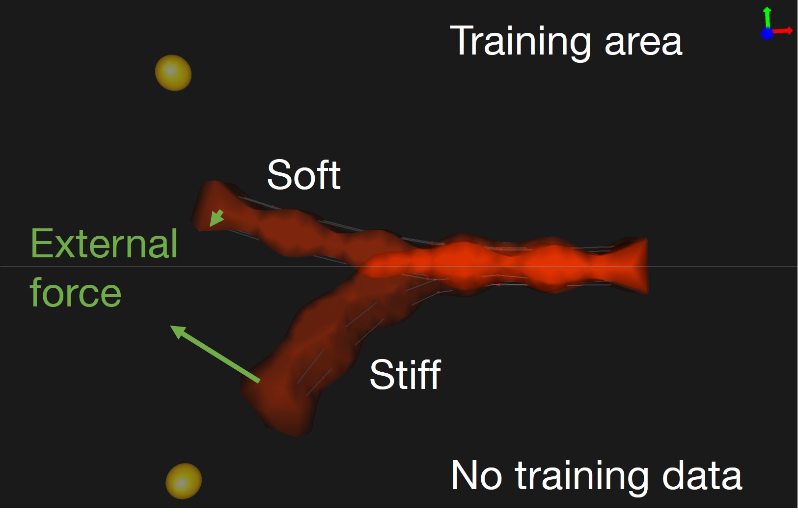
Figure 3: The robot remains soft in regions of high model confidence because of GP based feed-forward control. Video: https://youtu.be/vArJZukAzDA

Inside the training area, the robot is soft which is shown by a large deflection due to a small force (green arrow). In contrast, outside the training area, the stiffness is increasing due to the feedback control to keep the tracking error low.

IV Conclusion

We present a Gaussian Process based control law that keeps the robot soft without losing the tracking performance. For this purpose, an automatic weighting between feed-forward and feedback control based on the predicted variance of the GP is proposed. If the the robot operates inside an area of the workspace where training data was collected, the predicted mean of a GP is used as feed-forward control. Outside this area, the feedback part is getting more dominant that keeps the tracking error low but also increase the stiffness.

References

- Amiri Moghadam and Torabi [2016] A.A. Amiri Moghadam and K. et al. Torabi. Control-oriented modeling of a polymeric soft robot. Soft Robotics, 3(2), 2016. URL https://doi.org/10.1089/soro.2016.0002.
- Beckers et al. [2019] T. Beckers, D. Kulic, and S. Hirche. Stable Gaussian process based tracking control of Euler-Lagrange systems. Automatica, 103:390–397, 2019. URL https://doi.org/10.1016/j.automatica.2019.01.023.
- Bishop et al. [2006] Christopher M Bishop et al. Pattern recognition and machine learning, volume 4. Springer New York, 2006. URL https://www.springer.com/de/book/9780387310732.
- Bruder et al. [2019] Daniel Bruder, Brent Gillespie, C David Remy, and Ram Vasudevan. Modeling and control of soft robots using the koopman operator and model predictive control. arXiv preprint arXiv:1902.02827, 2019. URL https://arxiv.org/abs/1902.02827.
- Della Santina et al. [2017] Cosimo Della Santina, Matteo Bianchi, Giorgio Grioli, Franco Angelini, Manuel Catalano, Manolo Garabini, and Antonio Bicchi. Controlling soft robots: balancing feedback and feedforward elements. IEEE Robotics & Automation Magazine, 24(3):75–83, 2017. URL https://doi.org/10.1109/MRA.2016.2636360.
- Della Santina et al. [2018] Cosimo Della Santina, Robert K Katzschmann, Antonio Biechi, and Daniela Rus. Dynamic control of soft robots interacting with the environment. In 2018 IEEE International Conference on Soft Robotics (RoboSoft), pages 46–53. IEEE, 2018. URL https://doi.org/10.1109/ROBOSOFT.2018.8404895.
- Falkenhahn et al. [2015] Valentin Falkenhahn, Tobias Mahl, Alexander Hildebrandt, Rüdiger Neumann, and Oliver Sawodny. Dynamic modeling of bellows-actuated continuum robots using the euler–lagrange formalism. IEEE Transactions on Robotics, 31(6):1483–1496, 2015. URL https://doi.org/10.1109/TRO.2015.2496826.
- Fang et al. [2019] Ge Fang, Xiaomei Wang, Kui Wang, Kit-Hang Lee, Justin DL Ho, Hing-Choi Fu, Denny Kin Chung Fu, and Ka-Wai Kwok. Vision-based online learning kinematic control for soft robots using local gaussian process regression. IEEE Robotics and Automation Letters, 4(2):1194–1201, 2019. URL https://doi.org/10.1109/LRA.2019.2893691.
- Faure et al. [2012] François Faure, Christian Duriez, Hervé Delingette, Jérémie Allard, Benjamin Gilles, Stéphanie Marchesseau, Hugo Talbot, Hadrien Courtecuisse, Guillaume Bousquet, Igor Peterlik, and Stéphane Cotin. SOFA: A Multi-Model Framework for Interactive Physical Simulation, pages 283–321. Springer Berlin Heidelberg, 2012. URL https://doi.org/10.1007/8415_2012_125.
- Gillespie et al. [2018] Morgan T Gillespie, Charles M Best, Eric C Townsend, David Wingate, and Marc D Killpack. Learning nonlinear dynamic models of soft robots for model predictive control with neural networks. In 2018 IEEE International Conference on Soft Robotics (RoboSoft), pages 39–45. IEEE, 2018. URL https://doi.org/10.1109/ROBOSOFT.2018.8404894.
- Liu et al. [2018] Haitao Liu, Jianfei Cai, and Yew-Soon Ong. Remarks on multi-output gaussian process regression. Knowledge-Based Systems, 144:102–121, 2018. URL https://doi.org/10.1016/j.knosys.2017.12.034.
- Olguín-Díaz et al. [2018] Ernesto Olguín-Díaz, Christian A Trejo-Ramos, Vicente Parra-Vega, and David Navarro-Alarcón. On the modelling of soft-robots as quasi-continuum lagrangian dynamical systems with well-posed input matrix. arXiv preprint arXiv:1812.02738, 2018. URL https://arxiv.org/abs/1812.02738.
- Rasmussen and Williams [2006] Carl Edward Rasmussen and Christopher KI Williams. Gaussian processes for machine learning, volume 1. MIT press Cambridge, 2006. URL http://www.gaussianprocess.org/gpml/chapters/.
- Reinhart et al. [2017] René Reinhart, Zeeshan Shareef, and Jochen Steil. Hybrid analytical and data-driven modeling for feed-forward robot control. Sensors, 17(2):311, 2017. URL https://doi.org/10.3390/s17020311.
- Spong et al. [2006] Mark W Spong, Seth Hutchinson, and Mathukumalli Vidyasagar. Robot modeling and control, volume 3. wiley New York, 2006. URL https://www.wiley.com/en-us/Robot+Modeling+and+Control-p-9780471649908.