Renormalisation of pair correlations and their
Fourier transforms for primitive block substitutions

Abstract.

For point sets and tilings that can be constructed with the projection method, one has a good understanding of the correlation structure, and also of the corresponding spectra, both in the dynamical and in the diffraction sense. For systems defined by substitution or inflation rules, the situation is less favourable, in particular beyond the much-studied class of Pisot substitutions. In this contribution, the geometric inflation rule is employed to access the pair correlation measures of self-similar and self-affine inflation tilings and their Fourier transforms by means of exact renormalisation relations. In particular, we look into sufficient criteria for the absence of absolutely continuous spectral contributions, and illustrate this with examples from the class of block substitutions. We also discuss the Frank–Robinson tiling, as a planar example with infinite local complexity and singular continuous spectrum.

1. Introduction

The theory of model sets via the projection method, see [8, 56] and references therein for background, has led to a reasonably good understanding of mathematical models for perfect quasicrystals. This is particularly true of systems with pure point spectrum, and applies to spectra both in the diffraction and in the dynamical sense; see [8, 38, 40, 14, 13] and references therein for more, in particular on equivalence results for the different types of spectra.

Another intensely-studied approach starts from a substitution on a finite alphabet, or considers an inflation rule for a finite set of prototiles; see [8, 29, 55] and ¡ references therein for more. If the inflation multiplier happens to be a Pisot–Vijayaraghavan (PV) number, one meets an interesting overlap with the projection method via systems that can both be described by inflation and as a regular model set; see [8, Ch. 7] for some classic examples. However, the still open Pisot substitution conjecture, compare [1, 51], shows that important parts of the picture are still missing.

Considerably less is known for more general substitution or inflation schemes, be it beyond the PV case, in higher dimensions, or both. In particular, the study of non-PV substitutions is only at its beginning. Some recent progress [4, 6] in one dimension was possible by realising that such systems admit an exact renormalisation approach to their pair correlation measures; see [18, 19] for related results on the spectral measures for these systems.

The purpose of this contribution is to show how to extend such an exact renormalisation approach to higher dimensions, and also beyond the case of inflation tilings of finite local complexity (FLC). To be able to discuss some interesting classes of examples, we will build on several results from [6]. One of our goals is to formulate an effective sufficient criterion for the absence of absolutely continuous (ac) diffraction, which then implies that the diffraction measure is a singular measure, with the analogous result on the spectral measure of maximal type where possible at present. This clearly is expected to be the typical situation for inflation systems with vanishing topological entropy, but no general classification is known so far.

To formulate a criterion for the absence of ac components, it will be instrumental to identify a natural cocycle attached to the inflation rule together with an appropriate Lyapunov exponent. Implicitly, this amounts to an asymptotic analysis of infinite matrix products of Riesz product type. They have shown up in various ways in the spectral theory of inflation systems [48, 18, 4, 10, 19]. It should not be surprising to meet them again, in a slightly different fashion. In fact, they provide perhaps the most natural point of entry for a renormalisation type analysis of inflation systems.

This contribution is both a summary of known results, including those from [5, 44, 6, 3], and their extension to some new territory, in particular in higher dimensions (as announced in [45] and discussed in [6]). For the latter purpose, we proceed in an example-oriented manner via the class of block substitutions (not necessarily of constant size), which is still sufficiently simple to see the underlying ideas, yet rich enough to illustrate some new phenomena. In particular, in view of recent general interest [31, 32, 28, 33, 41, 55], we include some examples of infinite local complexity as well. Various general results that we employ are discussed and proved in [6], for which we only give a brief account here.

The material presented below is organised as follows. In Section 2, we set the scene by recalling some basic material, including some proofs for convenience, in particular where we are not aware of a good reference. Section 3 continues this account, covering some important aspects of uniform distribution and averages, which will be instrumental in most of our later calculations. Then, in Section 4, we discuss inflation systems in one dimension, from the viewpoint of exact renormalisation of the pair correlation measures and their Fourier transforms, with one concrete example of recent interest being discussed in Section 5. For further fully worked-out examples, we refer to [44, 5, 4, 10].

Starting with Section 6, we develop the entire theory for higher-dimensional inflation tilings with finitely many prototiles up to translations, which is then applied to various examples. In particular, we treat binary block substitutions of constant size (Section 7) and a rather versatile family of block substitutions with squares (Section 8), which comprises tilings with infinite local complexity. This is also a feature of the Frank–Robinson tiling (Section 9), which is shown to have singular continuous diffraction beyond the trivial Bragg peak at the origin. Some concluding remarks and open problems follow in Section 10.

2. Preliminaries

Our general references for concepts, notation and background are [8, 9]. Here, we collect further methods and results, where we begin with a simple property of Hermitian matrices.

Fact 2.1.

Let $H=(h_{ij})^{\phantom{a}}_{1\leqslant i,j\leqslant d}\in\operatorname{Mat}(d,\mathbb{C})$ be Hermitian and positive semi-definite, with rank $m$. Then, all diagonal elements of $H$ are non-negative. If $h_{ii}=0$ for some $i$, one has $h_{ij}=h_{ji}=0$ for all $1\leqslant j\leqslant d$. In particular, $H=0$ iff $m=0$.

Whenever $H\neq 0$, there are $m$ Hermitian, positive semi-definite matrices $H_{1},\ldots,H_{m}$ of rank $1$ such that $H=\sum_{r=1}^{m}H_{r}$ together with $H_{r}\hskip 0.5ptH_{s}=0$ for $r\neq s$.

Proof.

By Sylvester’s criterion, $H$ positive semi-definite means that all principal minors are non-negative, hence in particular all diagonal elements of $H$. Assume $h_{ii}=0$ for some $i$, and select any $j\in\{1,\ldots,d\}$. By semi-definiteness in conjunction with Hermiticity, one finds

$$0\,=\,h_{ii}\hskip 0.5pth_{jj}\,\geqslant\,h_{ij}\hskip 0.5pth_{ji}\,=\,\lvert h_{ij}\rvert^{2}\,\geqslant\,0\hskip 0.5pt,$$

which implies the second claim. The equivalence of $H=0$ with $m=0$ is clear.

Employing Dirac’s notation, the spectral theorem for Hermitian matrices asserts that one has $H=\sum_{i=1}^{d}|v_{i}\rangle\hskip 0.5pt\lambda_{i}\hskip 0.5pt\langle v_{i}|$, where the eigenvectors $|v_{i}\rangle$ can be chosen to form an orthonormal basis (so $\langle v_{i}|v_{j}\rangle=\delta_{i,j}$ and $|v_{i}\rangle\langle v_{i}|$ is a projector of rank $1$), while all eigenvalues are non-negative due to positive semi-definiteness. The rank of $H$ is the number of positive eigenvalues, counted with multiplicities. Ordering the eigenvalues decreasingly as $\lambda^{\phantom{a}}_{1}\geqslant\lambda^{\phantom{a}}_{2}\geqslant\cdots\geqslant\lambda^{\phantom{a}}_{d}\geqslant 0$, one can choose $H_{r}=|v_{r}\rangle\hskip 0.5pt\lambda_{r}\hskip 0.5pt\langle v_{r}|$ for $1\leqslant r\leqslant m$, and the claim is obvious. ∎

2.1. Logarithmic integrals and Mahler measures

The logarithmic Mahler measure of a polynomial $p\in\mathbb{C}[x]$ is defined as

(1) $$\mathfrak{m}\hskip 0.5pt(p)\,:=\int_{0}^{1}\log\big{|}p\bigl{(}\mathrm{e}^{2\pi\hskip 0.5pt\mathrm{i}\hskip 0.5ptt}\bigr{)}\big{|}\,\mathrm{d}t\hskip 0.5pt.$$

It was originally introduced by Mahler as a measure of the complexity of $p$; compare [25]. If $p(x)=a\prod_{i=1}^{s}(x-\alpha_{i})$, it follows from Jensen’s formula [49, Prop. 16.1] that

(2) $$\mathfrak{m}\hskip 0.5pt(p)\,=\,\log\hskip 0.5pt\lvert a\rvert\,+\sum_{i=1}^{s}\log\bigl{(}\max\{1,\lvert\alpha_{i}\rvert\}\bigr{)}.$$

This has the following immediate consequence.

Fact 2.2.

If $p$ is a monic polynomial that has no roots outside the unit disk, one has $\mathfrak{m}\hskip 0.5pt(p)=0$. In particular, this holds if $p$ is a cyclotomic polynomial, or a product of such a polynomial with a monomial. ∎

Clearly, for polynomials $p$ and $q$, one has $\mathfrak{m}\hskip 0.5pt(p\hskip 0.5ptq)=\mathfrak{m}\hskip 0.5pt(p)+\mathfrak{m}\hskip 0.5pt(q)$. If $p\in\mathbb{Z}\hskip 0.5pt[x]$, one can say more about the possible values of $\mathfrak{m}\hskip 0.5pt(p)$. They are of interest both in number theory and in dynamical systems; see [25, 3] and references therein.

Mahler measures of multivariate (or multi-variable) polynomials are defined by an integration over the corresponding torus. Concretely, for $p\in\mathbb{C}\bigl{[}x^{\phantom{a}}_{1},\ldots,x^{\phantom{a}}_{d}\bigr{]}$, one has

(3) $$\mathfrak{m}\hskip 0.5pt(p)\,:=\int_{\mathbb{T}^{d}}\log\big{|}p\bigl{(}\mathrm{e}^{2\pi\hskip 0.5pt\mathrm{i}\hskip 0.5ptt_{1}},\ldots,\mathrm{e}^{2\pi\hskip 0.5pt\mathrm{i}\hskip 0.5ptt_{d}}\bigr{)}\big{|}\,\mathrm{d}t^{\phantom{a}}_{1}\cdots\,\mathrm{d}t^{\phantom{a}}_{d}\hskip 0.5pt,$$

where $\mathbb{T}^{d}=\mathbb{R}^{d}/\mathbb{Z}\hskip 0.5pt^{d}$ denotes the $d$-torus. Unfortunately, in contrast to the one-dimensional situation, there is no simple general way to calculate such integrals. If we need to single out a variable, we do so by a subscript. For instance, $\mathfrak{m}\hskip 0.5pt_{x}(1+x+xy)$ denotes the logarithmic Mahler measure of $1+x+xy$, viewed as a polynomial in $x$, with $y$ being a coefficient. We refer to [25] for general background and examples.

2.2. Radon measures

Let $\mu$ denote a (generally complex) Radon measure on $\mathbb{R}^{d}$, which we primarily view as a linear functional over the space $C_{\mathsf{c}}(\mathbb{R}^{d})$ of compactly supported continuous functions. The ‘flipped-over’ version $\widetilde{\mu}$ is defined by $\widetilde{\mu}(g)=\overline{\mu(\widetilde{g}\hskip 0.5pt)}$, where $\widetilde{g}(x):=\overline{g(-x)}$. A measure $\mu$ is called positive when $\mu(g)\geqslant 0$ for all $g\geqslant 0$, and positive definite when $\mu(g*\widetilde{g}\hskip 0.5pt)\geqslant 0$ for all $g\in C_{\mathsf{c}}(\mathbb{R}^{d})$. Here, $g*h$ refers to the convolution of two integrable functions, as defined by $\bigl{(}g*h\bigr{)}(x)=\int_{\mathbb{R}^{d}}g(x-y)\hskip 0.5pth(y)\,\mathrm{d}y$. By $\lvert\mu\rvert$, we denote the total variation measure of $\mu$. If $\lvert\mu\rvert(\mathbb{R}^{d})<\infty$, the measure is bounded or finite, while we call it translation-bounded when $\sup_{t\in\mathbb{R}^{d}}\lvert\mu\rvert(t+K)<\infty$ holds for some compact set $K\subset\mathbb{R}^{d}$ with non-empty interior.

If $f\!:\,\mathbb{R}^{d}\xrightarrow{\quad}\mathbb{R}^{d}$ is an invertible mapping, we define the pushforward $f\!.\mu$ of a measure $\mu$ by $\bigl{(}f\!.\mu\bigr{)}(g)=\mu(g\circ\!f)$, where $g$ is an arbitrary test function. Viewing $\mu$ as a regular Borel measure via the general Riesz–Markov representation theorem, compare [50], the matching relation for a bounded Borel set $\mathcal{E}$ is

$$\bigl{(}f\!.\mu\bigr{)}(\mathcal{E})\,=\,\bigl{(}f\!.\mu\bigr{)}(1^{\phantom{a}}_{\mathcal{E}})\,=\,\mu(1^{\phantom{a}}_{\mathcal{E}}\circ f)\,=\,\mu\bigl{(}1^{\phantom{a}}_{f^{-1}(\mathcal{E})}\bigr{)}\,=\,\mu\bigl{(}f^{-1}(\mathcal{E})\bigr{)}.$$

Of particular importance is the Dirac measure at $x$, denoted by $\delta_{x}$, which is defined by $\delta_{x}(g)=g(x)$ for test functions. For Borel sets, the matching relation is

$$\delta^{\phantom{a}}_{x}(\mathcal{E})\,=\,\begin{cases}1,&\text{if $x\in\mathcal{E}$},\\ 0,&\text{otherwise},\end{cases}$$

which is often used in the form $\delta^{\phantom{a}}_{x}(\mathcal{E})=\delta^{\phantom{a}}_{x}\bigl{(}1^{\phantom{a}}_{\mathcal{E}}\bigr{)}$. For a point set $S\subset\mathbb{R}^{d}$, which is at most countable in our setting [8], one defines the corresponding Dirac comb as $\delta^{\phantom{a}}_{S}=\sum_{x\in S}\delta^{\phantom{a}}_{x}$.

When $\nu$ is absolutely continuous relative to $\mu$, denoted by $\nu\ll\mu$, with Radon–Nikodym density $h$, we write $\nu=h\hskip 0.5pt\mu$, so that $\bigl{(}h\hskip 0.5pt\mu\bigr{)}(g)=\mu(h\hskip 0.5ptg)$. For the pushforward, this leads to

(4) $$f\!.(h\hskip 0.5pt\mu)\,=\,\bigl{(}h\circ f^{-1}\bigr{)}\cdot(f\!.\mu)\hskip 0.5pt,$$

as follows from a simple calculation with a test function. When $f(x)=Ax$ with $A\in\mathrm{GL}(d,\mathbb{R})$ and $\mu$ is Lebesgue measure, it is sometimes more convenient to rewrite this relation as

(5) $$A.h\,:=\,f\!.h\,=\,\frac{h\circ f^{-1}}{\lvert\det(A)\rvert}\,=\,\frac{h\circ A^{-1}}{\lvert\det(A)\rvert}\hskip 0.5pt,$$

to be understood as a relation between absolutely continuous measures. The convolution $\mu*\nu$ of two finite measures is defined by

$$\bigl{(}\mu*\nu\bigr{)}(g)\,=\int_{\mathbb{R}^{d}}\int_{\mathbb{R}^{d}}g(x+y)\,\mathrm{d}\mu(x)\,\mathrm{d}\nu(y)\hskip 0.5pt,$$

which can be extended in various ways, in particular to the case where one measure is finite and the other is translation bounded [16, Prop. 1.13].

Lemma 2.3.

If $\mu$ and $\nu$ are convolvable measures on $\mathbb{R}^{d}$ and if $f\!:\,\mathbb{R}^{d}\xrightarrow{\quad}\mathbb{R}^{d}$ is invertible and linear, the pushforward operation satisfies $\,f\!.(\mu*\nu)=(f\!.\mu)*(f\!.\hskip 0.5pt\nu)$.

Proof.

Let $g$ be a general test function and define $g^{\phantom{a}}_{a}$ by $g^{\phantom{a}}_{a}(x)=g(a+x)$. Then, one has

$$\begin{split}\bigl{(}f\!.(\mu*\nu)\bigr{)}(g)\,&=\,\int_{\mathbb{R}^{d}}\int_{\mathbb{R}^{d}}g\bigl{(}f(x+y)\bigr{)}\,\mathrm{d}\mu(x)\,\mathrm{d}\nu(y)\,=\,\int_{\mathbb{R}^{d}}\int_{\mathbb{R}^{d}}g\bigl{(}f(x)+f(y)\bigr{)}\,\mathrm{d}\mu(x)\,\mathrm{d}\nu(y)\\[5.69054pt] &=\int_{\mathbb{R}^{d}}\mu\bigl{(}g^{\phantom{a}}_{f(y)}\circ f\bigr{)}\,\mathrm{d}\nu(y)\,=\int_{\mathbb{R}^{d}}(f\!.\mu)\bigl{(}g^{\phantom{a}}_{f(y)}\bigr{)}\,\mathrm{d}\nu(y)\\[5.69054pt] &=\int_{\mathbb{R}^{d}}\int_{\mathbb{R}^{d}}g\bigl{(}x+f(y)\bigr{)}\,\mathrm{d}\bigl{(}f\!.\mu\bigr{)}(x)\,\mathrm{d}\nu(y)\,=\int_{\mathbb{R}^{d}}\int_{\mathbb{R}^{d}}g^{\phantom{a}}_{x}\bigl{(}f(y)\bigr{)}\,\mathrm{d}\nu(y)\,\mathrm{d}\bigl{(}f\!.\mu\bigr{)}(x)\\[5.69054pt] &=\int_{\mathbb{R}^{d}}\nu(g^{\phantom{a}}_{x}\circ f)\,\mathrm{d}\bigl{(}f\!.\mu\bigr{)}(x)\,=\int_{\mathbb{R}^{d}}\bigl{(}f\!.\hskip 0.5pt\nu\bigr{)}(g^{\phantom{a}}_{x})\,\mathrm{d}\bigl{(}f\!.\mu\bigr{)}(x)\\[5.69054pt] &=\int_{\mathbb{R}^{d}}\int_{\mathbb{R}^{d}}g(x+y)\,\mathrm{d}\bigl{(}f\!.\hskip 0.5pt\nu\bigr{)}(y)\,\mathrm{d}\bigl{(}f\!.\mu\bigr{)}(x)\,=\,\bigl{(}(f\!.\hskip 0.5pt\nu)*(f\!.\mu)\bigr{)}(g)\\[8.53581pt] &=\,\bigl{(}(f\!.\mu)*(f\!.\hskip 0.5pt\nu)\bigr{)}(g)\hskip 0.5pt,\end{split}$$

where the second step in the third line, and the last step, rely on Fubini’s theorem. ∎

A linear map $f$ on $\mathbb{R}^{d}$ is expansive if there is a constant $\alpha>1$ such that $\|f(x)\|\geqslant\alpha\|x\|$ for all $x\in\mathbb{R}^{d}$. This implies that all eigenvalues satisfy $\lvert\lambda\rvert\geqslant\alpha$ and that $f$ is invertible.

Lemma 2.4.

Let $\mu$ be a Radon measure on $\mathbb{R}^{d}$ such that $\mu|^{\phantom{a}}_{U}=\mu(\{0\})\,\delta^{\phantom{a}}_{0}$ holds for some open neighbourhood $U$ of $0$. Then, if $f$ is an expansive linear map on $\mathbb{R}^{d}$, one has

$$\lim_{n\to\infty}f^{n}\!.\hskip 0.5pt\mu\,=\,\mu(\{0\})\,\delta^{\phantom{a}}_{0}\hskip 0.5pt.$$

Proof.

Let $\mathcal{E}\subset\mathbb{R}^{d}$ be a fixed, bounded Borel set. Viewing $\mu$ as a regular Borel measure, one has $\bigl{(}f^{n}\!.\mu\bigr{)}(\mathcal{E})=\mu\bigl{(}f^{-n}(\mathcal{E})\bigr{)}$. Since $f$ is expansive, with expansion constant $\alpha>1$, it is invertible, and $f^{-1}$ is contractive, with $\|f^{-1}(x)\|\leqslant\frac{1}{\alpha}\|x\|$ for all $x\in\mathbb{R}^{d}$. Consequently, $f^{-n}(\mathcal{E})\subset U$ for $n$ sufficiently large.

Now, the set $\mathcal{E}$ contains $0$ if and only if $f^{-n}(\mathcal{E})$ does, so $\bigl{(}f^{n}\!.\mu\bigr{)}(\mathcal{E})=\mu(\{0\})\,\delta^{\phantom{a}}_{0}(\mathcal{E})$ for $n$ large enough. Since $\mathcal{E}$ was bounded but otherwise arbitrary, our claim follows. ∎

The Fourier transform of measures will play an important role in many of our arguments. We follow the classical approach as outlined in [16, Ch. 1], see also [8, Ch. 8] as well as [46], where the Fourier transform of an integrable function $f$ is given by

$$\widehat{f}(k)\,=\int_{\mathbb{R}^{d}}\mathrm{e}^{-2\pi\hskip 0.5pt\mathrm{i}\hskip 0.5pt\langle k|x\rangle}f(x)\,\mathrm{d}x$$

as usual, where $\langle\cdot|\cdot\rangle$ denotes the standard inner product of $\mathbb{R}^{d}$. If $\mu$ is a finite measure, its Fourier transform is a continuous function, written as

$$\widehat{\mu}(k)\,=\int_{\mathbb{R}^{d}}\mathrm{e}^{-2\pi\hskip 0.5pt\mathrm{i}\hskip 0.5pt\langle k|x\rangle}\,\mathrm{d}\mu(x)\hskip 0.5pt.$$

For translation-bounded measures, we shall also employ standard notions and techniques from the theory of tempered distributions; compare [50, Sec. 6.2].

Below, we will make frequent use of a relation that tracks the consequence of an invertible linear map under Fourier transform.

Lemma 2.5.

Let $\mu$ be a Fourier-transformable measure on $\mathbb{R}^{d}$, and $A\in\mathrm{GL}(d,\mathbb{R})$. Then, with $A^{*}:=(A^{T})^{-1}$ denoting the dual matrix, one has

$$\widehat{A.\mu}\,=\,\frac{A^{*}\!.\hskip 0.5pt\widehat{\mu}}{\lvert\det(A)\rvert}\hskip 0.5pt.$$

Moreover, when $\widehat{\mu}$ is absolutely continuous relative to Lebesgue measure, hence represented by a locally integrable function, the relation simplifies to

$$\widehat{A.\mu}\,=\,\widehat{\mu}\hskip 0.5pt\circ A^{T}\,=\,A^{T}\!.\hskip 0.5pt\widehat{\mu}\hskip 0.5pt.$$

Proof.

If $g$ is an arbitrary test function, one has

$$\widehat{A.\mu}\,(g)\,=\,\bigl{(}A.\mu\bigr{)}(\hskip 0.5pt\widehat{g}\hskip 0.5pt)\,=\,\mu(\hskip 0.5pt\widehat{g}\circ A)\,=\int_{\mathbb{R}^{d}}\int_{\mathbb{R}^{d}}\mathrm{e}^{-2\pi\hskip 0.5pt\mathrm{i}\hskip 0.5pt\langle x|At\rangle}g(x)\,\mathrm{d}x\,\mathrm{d}\mu(t)\hskip 0.5pt.$$

Observing $\langle x|A\hskip 0.5ptt\rangle=\langle t|A^{T}x\rangle$ and setting $x=A^{*}y$, hence $\,\mathrm{d}x=\lvert\det(A^{*})\rvert\,\mathrm{d}y$, one finds

$$\begin{split}\widehat{A.\mu}\,(g)\,&=\int_{\mathbb{R}^{d}}\int_{\mathbb{R}^{d}}\mathrm{e}^{-2\pi\hskip 0.5pt\mathrm{i}\hskip 0.5pt\langle t|y\rangle}g(A^{*}y)\,\frac{\,\mathrm{d}y\,\mathrm{d}\mu(t)}{\lvert\det(A)\rvert}\,=\int_{\mathbb{R}^{d}}\bigl{(}\widehat{g\circ A^{*}}\bigr{)}(t)\frac{\,\mathrm{d}\mu(t)}{\lvert\det(A)\rvert}\\[5.69054pt] &=\,\frac{\mu\bigl{(}\widehat{g\circ A^{*}}\bigr{)}}{\lvert\det(A)\rvert}\,=\,\frac{\widehat{\mu}\bigl{(}g\circ A^{*}\bigr{)}}{\lvert\det(A)\rvert}\,=\,\frac{\bigl{(}A^{*}\!.\hskip 0.5pt\widehat{\mu}\bigr{)}(g)}{\lvert\det(A)\rvert}\hskip 0.5pt,\end{split}$$

which implies the first claim. The second is now a consequence of Eq. (5). ∎

2.3. Riesz products

Of particular interest in the context of singular measures are measures that have a representation as infinite Riesz products. Let us recall one paradigmatic example of pure point type, and then generalise it. Here, an expression of the form $\prod_{m\geqslant 0}f_{m}(k)$ with continuous functions $f_{m}$ is a short-hand for the measure that is defined as the vague limit of a sequence of absolutely continuous measures, the latter being given by the Radon–Nikodym densities $\prod_{m=0}^{n}f_{m}(k)$ with $n\geqslant 0$.

Lemma 2.6.

As a relation between translation-bounded measures on $\mathbb{R}$, one has

$$\prod_{m\geqslant 0}\bigl{(}1+\cos(2\pi\hskip 0.5pt2^{m}k)\bigr{)}\,=\,\delta^{\phantom{a}}_{\mathbb{Z}\hskip 0.5pt}\hskip 0.5pt,$$

where $k\in\mathbb{R}$ and convergence is in the vague topology.

Proof.

We employ a method that is well known from the theory of Bernoulli convolutions; compare [47]. Define $\mu=\delta^{\phantom{a}}_{0}+\delta^{\phantom{a}}_{1}$ and consider $\nu=\frac{1}{2}\,\mu*\widetilde{\mu}=\delta^{\phantom{a}}_{0}+\frac{1}{2}(\delta^{\phantom{a}}_{1}+\delta^{\phantom{a}}_{-1})$, so

$$\widehat{\nu}(k)\,=\,1+\cos(2\pi k)\hskip 0.5pt.$$

With $f(x)=2x$, one has $f\!.\hskip 0.5pt\nu=\frac{1}{2}\,(f\!.\mu)*(f\!.\widetilde{\mu}\hskip 0.5pt)$ by Lemma 2.3, where $f\!.\widetilde{\mu}=\widetilde{f\!.\mu\,}$. Moreover, one has $\mu*(f\!.\mu)*\ldots*(f^{n-1}\!.\mu)=\sum_{\ell=0}^{2^{n}-1}\delta^{\phantom{a}}_{\ell}$. Now, for $n\geqslant 1$, a simple convolution calculation gives

$$\operatorname*{\text{\Huge\raisebox{-3.5pt}{$\ast$}}}_{m=0}^{n-1}f^{m}\!.\hskip 0.5pt\nu\,=\sum_{\ell=1-2^{n}}^{2^{n}-1}\!\frac{\raisebox{-2.0pt}{$2^{n}-\lvert\ell\rvert$}}{\raisebox{0.5pt}{$2^{n}$}}\,\delta^{\phantom{a}}_{\ell}\;\xrightarrow{\,n\to\infty\,}\;\delta^{\phantom{a}}_{\mathbb{Z}\hskip 0.5pt}\hskip 0.5pt,$$

with convergence in the vague topology.

With $\widehat{f^{m}_{\vphantom{I}}\!.\hskip 0.5pt\nu}=\widehat{\nu}\circ f^{m}$, which follows from Lemma 2.5, an application of the convolution theorem in conjunction with the continuity of the Fourier transform leads to

(6) $$\widehat{\operatorname*{\text{\Huge\raisebox{-3.5pt}{$\ast$}}}_{m=0}^{n-1}f^{m}\!.\hskip 0.5pt\nu}\,=\prod_{m=0}^{n-1}(\widehat{\nu}\circ f^{m})\;\xrightarrow{\,n\to\infty\,}\;\widehat{\hskip 0.5pt\delta^{\phantom{a}}_{\mathbb{Z}\hskip 0.5pt}\hskip 0.5pt}\,=\,\delta^{\phantom{a}}_{\mathbb{Z}\hskip 0.5pt}\hskip 0.5pt,$$

where the last step is the Poisson summation formula (PSF); compare [8, Prop. 9.4]. Our claim now follows via the observation that $\bigl{(}\widehat{\nu}\circ f^{m}\bigr{)}(k)=1+\cos(2\pi\hskip 0.5pt2^{m}k)$. ∎

More generally, let $2\leqslant M\in\mathbb{N}$ be fixed and consider

$$\mu\,=\sum_{\ell=0}^{M-1}\delta^{\phantom{a}}_{\ell}\quad\text{and}\quad\nu\,=\,\frac{\mu*\widetilde{\mu}}{M}\,=\,\delta^{\phantom{a}}_{0}\,+\sum_{\ell=1}^{M-1}\frac{\raisebox{-2.0pt}{$M-\ell$}}{\raisebox{0.5pt}{$M$}}\bigl{(}\delta^{\phantom{a}}_{\ell}+\delta^{\phantom{a}}_{-\ell}\bigr{)}.$$

With $f(x)=Mx$, one has $\mu*(f\!.\mu)*\ldots*(f^{n-1}\!.\mu)=\sum_{\ell=0}^{M^{n}-1}\delta^{\phantom{a}}_{\ell}$ and

$$\operatorname*{\text{\Huge\raisebox{-3.5pt}{$\ast$}}}_{m=0}^{n-1}f^{m}\!.\nu\,=\sum_{\ell=1-M^{n}}^{M^{n}-1}\!\frac{\raisebox{-2.0pt}{$M^{n}-\lvert\ell\rvert$}}{\raisebox{0.5pt}{$M^{n}$}}\,\delta^{\phantom{a}}_{\ell}\;\xrightarrow{\,n\to\infty\,}\;\delta^{\phantom{a}}_{\mathbb{Z}\hskip 0.5pt}$$

in the vague topology, so that Eq. (6) holds here as well. Observe that

$$\widehat{\nu}(k)\,=\,1+2\sum_{\ell=1}^{M-1}\frac{\raisebox{-2.0pt}{$M-\ell$}}{\raisebox{0.5pt}{$M$}}\,\cos(2\pi\ell k)\hskip 0.5pt,$$

which satisfies $\widehat{\nu}(k)\geqslant 0$ and $\int_{0}^{1}\widehat{\nu}(k)\,\mathrm{d}k=1$. Moreover, $\prod_{m=0}^{n-1}\bigl{(}\widehat{\nu}\circ f^{m}\bigr{)}$ defines a probability density on $[0,1]$ for each $n\in\mathbb{N}$. Now, the generalisation of Lemma 2.6 reads as follows.

Proposition 2.7.

For any $2\leqslant M\in\mathbb{N}$, one has

$$\prod_{m\geqslant 0}\Bigl{(}1+\hskip 0.5pt2\sum_{\ell=1}^{M-1}\frac{\raisebox{-2.0pt}{$M-\ell$}}{\raisebox{0.5pt}{$M$}}\,\cos(2\pi\ell M^{m}k)\Bigr{)}\,=\,\delta^{\phantom{a}}_{\mathbb{Z}\hskip 0.5pt}\hskip 0.5pt,$$

where $k\in\mathbb{R}$ and convergence is in the vague topology. ∎

It is clear how to extend this to more than one dimension, the details of which are left to the interested reader.

3. Uniform distribution and averages

While uniform distribution results are usually stated for one dimension, many of them have natural, though less well-known, generalisations to higher dimensions. We shall need some of them to calculate limits of various Birkhoff sums in our examples. To formulate the results, we represent $\mathbb{T}^{d}=\mathbb{R}^{d}/\mathbb{Z}\hskip 0.5pt^{d}$ as the half-open unit cube $[0,1)^{d}$ with (coordinate -wise) addition modulo $1$. As before, we use $\langle x\hskip 0.5pt|\hskip 0.5pty\rangle=\sum_{i=1}^{d}x_{i}\hskip 0.5pty_{i}$ for the standard inner product in $\mathbb{R}^{d}$. Let us recall some useful properties of non-singular linear forms.

Fact 3.1.

Consider a non-singular linear form $f\!:\,\mathbb{R}^{d}\xrightarrow{\quad}\mathbb{R}$, which can thus be written as $f(x)=\langle a\hskip 0.5pt|\hskip 0.5ptx\rangle$ with $0\neq a\in\mathbb{R}^{d}$. Then, if $\mathcal{E}$ is a Lebesgue null set in $\mathbb{R}$, its preimage $f^{-1}(\mathcal{E})$ is a Lebesgue null set in $\mathbb{R}^{d}$.

Proof.

Let $\mu^{\phantom{a}}_{\mathrm{L}}$ and $\nu^{\phantom{a}}_{\mathrm{L}}$ denote Lebesgue measure in $\mathbb{R}^{d}$ and $\mathbb{R}$, respectively. Clearly, the linear mapping $f$ is differentiable, with $\nabla f(x)=a\neq 0$ for all $x\in\mathbb{R}^{d}$, hence certainly measurable and surjective. Now, the pushforward $f\!.\mu^{\phantom{a}}_{\mathrm{L}}$ defines a regular Borel measure on $\mathbb{R}$, with $\bigl{(}f\!.\mu^{\phantom{a}}_{\mathrm{L}}\bigr{)}(\mathcal{E})=\mu^{\phantom{a}}_{\mathrm{L}}\bigl{(}f^{-1}(\mathcal{E})\bigr{)}$ for any Borel set $\mathcal{E}\subseteq\mathbb{R}$; compare [36, Thm. 39.C]. Due to the linearity of $f$, for any $t\in\mathbb{R}$, we have $f^{-1}(t+\mathcal{E})=z^{\phantom{a}}_{t}+f^{-1}(\mathcal{E})$ for some $z^{\phantom{a}}_{t}\in\mathbb{R}^{d}$ with $f(z^{\phantom{a}}_{t})=t$, which covers the empty set via the standard convention $x+\varnothing=\varnothing$.

This property implies $\bigl{(}f\!.\mu^{\phantom{a}}_{\mathrm{L}}\bigr{)}(t+\mathcal{E})=\bigl{(}f\!.\mu^{\phantom{a}}_{\mathrm{L}}\bigr{)}(\mathcal{E})$ for all $t\in\mathbb{R}$ and all Borel sets $\mathcal{E}$, which means that $f\!.\mu^{\phantom{a}}_{\mathrm{L}}$ is translation invariant and thus a multiple of Haar measure on $\mathbb{R}$. Consequently, we have $f\!.\mu^{\phantom{a}}_{\mathrm{L}}=c\hskip 0.5pt\hskip 0.5pt\nu^{\phantom{a}}_{\mathrm{L}}$, where $c>0$ follows from $a\neq 0$. This means that $f\!.\mu^{\phantom{a}}_{\mathrm{L}}$ and $\nu^{\phantom{a}}_{\mathrm{L}}$ are equivalent as measures, and our claim on the Lebesgue null sets follows. ∎

Fact 3.2.

Let $\alpha\in\mathbb{R}$ with $\lvert\alpha\rvert>1$ be given and let $f$ be the linear form from Fact 3.1. Then, for Lebesgue-a.e. $x\in\mathbb{R}^{d}$, the sequence $\bigl{(}f(\alpha^{n}x)\bigr{)}_{n\in\mathbb{N}}$ is uniformly distributed modulo $1$.

Proof.

One has $f(\alpha^{n}x)=\alpha^{n}\hskip 0.5ptt$ with $t=\langle a\hskip 0.5pt|\hskip 0.5ptx\rangle$ and $a\neq 0$. Clearly, $(\alpha^{n}\hskip 0.5ptt)^{\phantom{a}}_{n\in\mathbb{N}}$ is uniformly distributed modulo $1$ for a.e. $t\in\mathbb{R}$ by standard results from uniform distribution theory; compare [39, Thm. 4.3 and Exc. 4.3]. If $\mathcal{E}$ is the corresponding null set of exceptional points, uniform distribution modulo $1$ of $\bigl{(}f(\alpha^{n}x)\bigr{)}_{n\in\mathbb{N}}$ fails precisely for all $x\in f^{-1}(\mathcal{E})\subset\mathbb{R}^{d}$. By Fact 3.1, $f^{-1}(\mathcal{E})$ is a null set in $\mathbb{R}^{d}$, which implies the claim. ∎

Lemma 3.3.

Let $\alpha\in\mathbb{R}$ with $\lvert\alpha\rvert>1$ be fixed. Then, for Lebesgue-a.e. $x\in\mathbb{R}^{d}$, the sequence $(\alpha^{n}x)^{\phantom{a}}_{n\in\mathbb{N}}$ taken modulo $1$ is uniformly distributed in $\mathbb{T}^{d}$.

Proof.

For $d=1$, this is a well-known result from metric equidistribution theory [39, Ch. 4], as mentioned earlier. For $d>1$ and any given $x\in\mathbb{R}^{d}$, it is convenient to employ Weyl’s criterion [39, Thm. 6.2] and consider the convergence behaviour of character sums. In fact, this implies that uniform distribution of $(\alpha^{n}x)^{\phantom{a}}_{n\in\mathbb{N}}$ modulo $1$ is equivalent to uniform distribution modulo $1$ of the sequences $(\alpha^{n}\langle k\hskip 0.5pt|\hskip 0.5ptx\rangle)^{\phantom{a}}_{n\in\mathbb{N}}$ for all $k\in\mathbb{Z}\hskip 0.5pt^{d}\setminus\{0\}$; compare [39, Thm. 6.3]. For each such $k$, let $\mathcal{E}_{k}$ be the exceptional set of points $x\in\mathbb{R}^{d}$ where uniform distribution fails, which is a null set by Fact 3.2. Since $\mathbb{Z}\hskip 0.5pt^{d}\setminus\{0\}$ is countable, the set $\bigcup_{k\in\mathbb{Z}\hskip 0.5pt^{d}\setminus\{0\}}\mathcal{E}_{k}$ is still a null set in $\mathbb{R}^{d}$, and the claim follows. ∎

Next, we need to understand averages of various types of periodic and almost periodic functions, in particular along exponential sequences of the above type.

Lemma 3.4.

Let $\alpha\in\mathbb{R}$ with $\lvert\alpha\rvert>1$ be fixed. For any $a\in\mathbb{R}^{d}$ and then a.e. $x\in\mathbb{R}^{d}$, one has

$$\lim_{N\to\infty}\frac{\raisebox{-2.0pt}{$1$}}{\raisebox{0.5pt}{$N$}}\sum_{n=0}^{N-1}\mathrm{e}^{2\pi\hskip 0.5pt\mathrm{i}\hskip 0.5pt\hskip 0.5pt\alpha^{n}\langle a\hskip 0.5pt|\hskip 0.5ptx\rangle}\,=\,\delta^{\phantom{a}}_{a,0}\hskip 0.5pt.$$

Proof.

When $a=0$, the limit is $1$ for all $x\in\mathbb{R}^{d}$, so let $a\neq 0$. Then, by Fact 3.2, $(\alpha^{n}\langle a\hskip 0.5pt|\hskip 0.5ptx\rangle)^{\phantom{a}}_{n\in\mathbb{N}}$ is uniformly distributed modulo $1$ for a.e. $x\in\mathbb{R}^{d}$, where the null set $\mathcal{E}_{a}$ of exceptions depends on $a$. So, for any given $a$ and then every $x\in\mathbb{R}^{d}\setminus\mathcal{E}_{a}$, we get

$$\lim_{N\to\infty}\frac{\raisebox{-2.0pt}{$1$}}{\raisebox{0.5pt}{$N$}}\sum_{n=0}^{N-1}\mathrm{e}^{2\pi\hskip 0.5pt\mathrm{i}\hskip 0.5pt\hskip 0.5pt\alpha^{n}\langle a\hskip 0.5pt|\hskip 0.5ptx\rangle}\,=\int_{0}^{1}\mathrm{e}^{2\pi\hskip 0.5pt\mathrm{i}\hskip 0.5ptt}\,\mathrm{d}t\,=\,0$$

by Weyl’s lemma. ∎

The next step is an extension to (complex) trigonometric polynomials, as given by

$$P_{m}(x)\,=\,c^{\phantom{a}}_{\hskip 0.5pt0}\,+\sum_{\ell=1}^{m}c^{\phantom{a}}_{\ell}\,\mathrm{e}^{2\pi\hskip 0.5pt\mathrm{i}\hskip 0.5pt\hskip 0.5pt\langle k_{\ell}\hskip 0.5pt|\hskip 0.5ptx\rangle}$$

with $m\in\mathbb{N}_{0}$ and coefficients $c^{\phantom{a}}_{\ell}\in\mathbb{C}$. When $m\geqslant 1$, the frequency vectors $k^{\phantom{a}}_{1},\ldots,k^{\phantom{a}}_{m}$ are assumed to be non-zero and distinct. Clearly, under the conditions of Lemma 3.4, one obtains

(7) $$\lim_{N\to\infty}\frac{\raisebox{-2.0pt}{$1$}}{\raisebox{0.5pt}{$N$}}\sum_{n=0}^{N-1}P_{m}(\alpha^{n}x)\,=\,c^{\phantom{a}}_{\hskip 0.5pt0}\,=\,\mathbb{M}(P_{m})$$

for a.e. $x\in\mathbb{R}^{d}$. Here, $\mathbb{M}(f)$ is the mean of a bounded function,

(8) $$\mathbb{M}(f)\,:=\,\lim_{n\to\infty}\frac{\raisebox{-2.0pt}{$1$}}{\raisebox{0.5pt}{$\operatorname{vol}(A_{n})$}}\int_{A_{n}}f(x)\,\mathrm{d}x\hskip 0.5pt,$$

where $\mathcal{A}=(A_{n})^{\phantom{a}}_{n\in\mathbb{N}}$ is a fixed sequence of growing sets for the averaging process. The sets $A_{n}$ are supposed to be sufficiently ‘nice’, which means that one assumes a property of Følner or van Hove type. To be concrete, we can think of $A_{n}$ as the closed cube of sidelength $n$ centred at $0$. It is clear that the limit in (8) exists for trigonometric polynomials. More generally, it exists for all functions that are uniformly almost periodic, which are often also called Bohr almost periodic. They are the continuous functions that can uniformly be approximated by trigonometric polynomials. In other words, the space of uniformly almost periodic functions is the $\|.\|^{\phantom{a}}_{\infty}$-closure of the space of trigonometric polynomials; see [23] for general results.

Proposition 3.5.

Let $f\!:\,\mathbb{R}^{d}\xrightarrow{\quad}\mathbb{C}$ be a uniformly $($or Bohr$\,)$ almost periodic function, and let $\alpha\in\mathbb{R}$ with $\lvert\alpha\rvert>1$ be given. Then, for a.e. $x\in\mathbb{R}^{d}$, one has

$$\lim_{N\to\infty}\frac{\raisebox{-2.0pt}{$1$}}{\raisebox{0.5pt}{$N$}}\sum_{n=0}^{N-1}f(\alpha^{n}x)\,=\,\mathbb{M}(f)\hskip 0.5pt.$$

In particular, this applies to functions of the form $f=\log(g)$ with $g$ a non-negative, uniformly almost periodic function that is bounded away from $0$.

Proof.

The first claim for $d=1$ is [11, Thm. 6.4.4]. A close inspection of its proof reveals that the same chain of arguments also applies to the case $d>1$, which is all we need here.

The second claim follows from the first because $g(x)\geqslant\delta>0$ for all $x\in\mathbb{R}^{d}$ implies that $\log(g)$ is again a uniformly almost periodic function [4, Fact 6.14]. ∎

In the attempt to generalise Proposition 3.5 beyond uniformly almost periodic functions, one difficulty emerges when $f$ is no longer locally Riemann-integrable. Let us first look at periodic functions, where we begin by recalling a classic result.

Fact 3.6 ([11, Lemma 6.3.3]).

Let $q\in\mathbb{Z}\hskip 0.5pt$ with $\lvert q\rvert\geqslant 2$ be fixed, and consider a function $f\in L^{1}_{\mathrm{loc}}(\mathbb{R})$ that is $1$-periodic. Then,

$$\frac{\raisebox{-2.0pt}{$1$}}{\raisebox{0.5pt}{$N$}}\sum_{n=0}^{N-1}f(q^{n}x)\,\xrightarrow{\,N\to\infty\,}\int_{0}^{1}\!f(y)\,\mathrm{d}y\,=\,\mathbb{M}(f)$$

holds for a.e. $x\in\mathbb{R}$. ∎

The key ingredient to Fact 3.6 is the ergodicity of Lebesgue measure on $\mathbb{T}$ for the dynamical system defined by $x\mapsto qx$ modulo $1$, which permits to use Birkhoff’s ergodic theorem instead of Weyl’s lemma and uniform distribution of $(q^{n}x)^{\phantom{a}}_{n\in\mathbb{N}}$ for a.e. $x\in\mathbb{R}$. The natural counterpart on $\mathbb{T}^{d}$ can be stated as follows.

Lemma 3.7.

Let $Q$ be a non-singular endomorphism of $\mathbb{T}^{d}$ such that no eigenvalue is a root of unity, and consider a $\mathbb{Z}\hskip 0.5pt^{d}$-periodic function $f\in L^{1}_{\mathrm{loc}}(\mathbb{R}^{d})$. Then, for a.e. $x\in\mathbb{R}^{d}$, one has

$$\frac{\raisebox{-2.0pt}{$1$}}{\raisebox{0.5pt}{$N$}}\sum_{n=0}^{N-1}f(Q^{n}x)\,\xrightarrow{\,N\to\infty\,}\int_{\mathbb{T}^{d}}f(y)\,\mathrm{d}y\,=\,\mathbb{M}(f)\hskip 0.5pt.$$

In particular, this result applies to every toral endomorphism that is expansive.

Proof.

Under our assumptions, Lebesgue measure is an invariant and ergodic measure for the dynamical system defined by $Q$ on $\mathbb{T}^{d}$; see [24, Cor. 2.20]. The main statement now follows from Birkhoff’s ergodic theorem. Since all eigenvalues of an expansive $Q\in\mathrm{End}(\mathbb{T}^{d})$ satisfy $\lvert\lambda\rvert>1$, the last claim is clear. ∎

Beyond Fact 3.6 and Lemma 3.7, we will need the following result, which can be viewed as a variant of Sobol’s theorem [52]; see also [37, 11].

Lemma 3.8.

Let $p\geqslant 0$ be a trigonometric polynomial in $d$ variables, and let $\alpha\in\mathbb{R}$ with $\lvert\alpha\rvert>1$ be fixed. Let us further assume that, for some sufficiently small $\delta>0$, the critical points of $p$ with value in $[0,\delta]$ are isolated. Then, for Lebesgue-a.e. $x\in\mathbb{R}^{d}$, one has

$$\lim_{N\to\infty}\frac{\raisebox{-2.0pt}{$1$}}{\raisebox{0.5pt}{$N$}}\sum_{n=0}^{N-1}\log\bigl{(}p(\alpha^{n}x)\bigr{)}\,=\,\mathbb{M}\bigl{(}\log(p)\bigr{)}.$$

Sketch of proof.

Since the case $p(k)\geqslant\delta>0$ for all $k\in\mathbb{R}^{d}$ is covered by Proposition 3.5, we assume $\inf_{k\in\mathbb{R}^{d}}p(k)=0$ and thus $\inf_{k\in\mathbb{R}^{d}}\log(p(k))=-\infty$, which is the origin of the complication. Note, however, that all singularities of $\log({p})$ are of logarithmic type and hence locally integrable, so $\log(p)$ is no longer uniformly, but still Stepanov almost periodic; compare [11, pp. 356–359] as well as [23, Sec. VI.4].

Now, we have to deal with the small local minima of $p$. By assumption, there is a $\delta>0$ such that the points $k$ with $\nabla p(k)=0$ and $p(k)\in[0,\delta]$ are isolated. As $p$ is a quasiperiodic function, the set of critical points of this type, $Z$ say, must then be uniformly discrete.

Now, with a Borel–Cantelli argument, compare [11, Thm. 6.3.5] and [10, Prop. 5.1], one can derive that, for a.e. $x\in\mathbb{R}^{d}$, the sequence $(\alpha^{n}x)^{\phantom{a}}_{n\in\mathbb{N}_{0}}$ stays sufficiently far away from $Z$ so that the average via the Birkhoff sum ultimately is not distorted by the singularities or almost singularities of $\log(p)$, and Sobol’s theorem can be applied. This gives

$$\lim_{N\to\infty}\frac{\raisebox{-2.0pt}{$1$}}{\raisebox{0.5pt}{$N$}}\sum_{n=0}^{N-1}\log\bigl{(}{p}(\alpha^{n}x)\bigr{)}\,=\,\mathbb{M}\bigl{(}\log(p)\bigr{)}$$

for a.e. $x\in\mathbb{R}^{d}$ as claimed. ∎

At this point, we are set to start the spectral analysis of inflation systems via their pair correlations, where we begin with the theory in one dimension.

4. Results in one dimension

Let us recall the situation in one dimension from [5, 6]. Consider a primitive substitution $\varrho$ on an $L$-letter alphabet $\mathcal{A}=\{a^{\phantom{a}}_{1},\dots,a^{\phantom{a}}_{L}\}$. It defines a unique symbolic hull $\mathbb{X}_{\varrho}$, which is compact and consists of a single local indistinguishability (LI) class. This hull can be constructed as the closure of the shift orbit of a two-sided fixed point of a suitable power of $\varrho$. This shift space gives rise to a uniquely (in fact, strictly) ergodic dynamical system under the $\mathbb{Z}\hskip 0.5pt$-action of the shift, denoted as $(\mathbb{X}_{\varrho},\mathbb{Z}\hskip 0.5pt)$.

The corresponding substitution matrix $M$ is the primitive non-negative $L\!\times\!L$-matrix with elements $M_{ij}=\operatorname{card}_{a^{\phantom{a}}_{i}}\bigl{(}\varrho(a^{\phantom{a}}_{j})\bigr{)}$ and Perron–Frobenius (PF) eigenvalue $\lambda>1$. The matching (properly normalised) right eigenvector of $M$ encodes the letter frequencies, while the left eigenvector determines the ratios of natural tile lengths for a consistent geometric inflation rule. The latter acts on $L$ intervals (which are our prototiles), one for each letter, of lengths corresponding to the entries of the left eigenvector. If the $L$ intervals do not have distinct lengths, we distinguish congruent ones by labels (or colours). The inflation map induced by $\varrho$ then consists of a scaling of the intervals by the inflation multiplier $\lambda$ and their subsequent dissection into original prototiles, according to the order determined by the substitution rule $\varrho$. In this setting, the inflation again defines a strictly ergodic dynamical system, now (in general) under the continuous translation action of $\mathbb{R}$, denoted as $(\mathbb{Y},\mathbb{R})$, with $\mathbb{Y}$ the new tiling hull.

To capture the geometric information, let us collect the relative positions of the tiles in the inflation map in a set-valued displacement matrix $T$. Each element $T_{ij}$ thus is a set, viewed as a list of length $M_{ij}$ that contains the relative positions of the interval (or tile) of type $i$ in the inflated interval (or supertile) of type $j$ (and is the empty set if $M_{ij}=0$). To define the distance between tiles, we assign a reference point to each tile, which we usually choose to be the left endpoint of the interval. Clearly, since the reference point determines the tile and its position, the set of (labelled or coloured) reference points is mutually locally derivable (MLD) with the tiling by intervals. For a given tiling, define $\varLambda_{i}$ as the set of all reference points of tiles of type $i$, and $\varLambda=\dot{\bigcup}_{i=1}^{L}\varLambda_{i}$ as the set of all such reference points.

Let $\nu^{\phantom{a}}_{ij}(z)$ with $z\geqslant 0$ be the relative frequency of the occurrence of a tile of type $i$ (left) and one of type $j$ (right) at distance $z$, with the understanding that $\nu^{\phantom{a}}_{ij}(-z)=\nu^{\phantom{a}}_{ji}(z)$. These are the pair correlation coefficients of the inflation rule, which exist for all elements of the hull and are independent of the choice of the element. Given $\varLambda$, decomposed as $\varLambda=\dot{\bigcup}_{i}\varLambda_{i}$, one can represent each coefficient as a limit,

$$\nu^{\phantom{a}}_{ij}(z)\,=\lim_{r\to\infty}\frac{\operatorname{card}\bigl{(}B_{r}(0)\cap\varLambda_{i}\cap(\varLambda_{j}-z)\bigr{)}}{\operatorname{card}(B_{r}(0)\cap\varLambda)}\,=\,\frac{\operatorname{dens}\bigl{(}\varLambda_{i}\cap(\varLambda_{j}-z)\bigr{)}}{\operatorname{dens}(\varLambda)}\,\geqslant\,0\hskip 0.5pt.$$

Due to the strict ergodicity, one has $\nu^{\phantom{a}}_{ij}(z)>0$ if and only if $z\in S_{ij}:=\varLambda_{j}-\varLambda_{i}$, where the sets $S_{ij}$ are independent of the choice of $\varLambda$ from the hull, because the latter is minimal and thus consists of a single LI class [8].

Let us now recall the general renormalisation relations for the $\nu^{\phantom{a}}_{ij}$ from [5, 4, 10], which are proved in full generality in [6], also for higher dimensions; see Eq. (18) below.

Lemma 4.1.

Let $\nu^{\phantom{a}}_{ij}$ be the pair correlation coefficients of the geometric inflation rule induced by the primitive $L$-letter substitution $\varrho$ with inflation multiplier $\lambda$, and let $T$ be the corresponding set-valued displacement matrix. Then, they satisfy the identities

$$\nu^{\phantom{a}}_{ij}(z)\,=\,\frac{\raisebox{-2.0pt}{$1$}}{\raisebox{0.5pt}{$\lambda$}}\sum_{m,n=1}^{L}\,\sum_{r\in T_{im}}\,\sum_{s\in T_{jn}}\nu^{\phantom{a}}_{mn}\left(\frac{\raisebox{-2.0pt}{$z+r-s$}}{\raisebox{0.5pt}{$\lambda$}}\right)$$

for arbitrary $z\in\mathbb{R}$. ∎

Remark 4.2.

The identities of Lemma 4.1 have a special structure, which we call an exact renormalisation for the following reason. First, there is a finite subset of identities that close, and give what is known as the self-consistency part of the identities. Then, all remaining relations are purely recursive, which also implies that the solution space of the renormalisation identities is finite-dimensional. This is further discussed and explored in [5, 6]. $\Diamond$

Now, define $\varUpsilon^{\phantom{a}}_{ij}=\sum_{z\in S_{ij}}\nu^{\phantom{a}}_{ij}(z)\,\delta^{\phantom{a}}_{z}$, which is a pure point measure for each $1\leqslant i,j\leqslant L$. For the measure vector $\varUpsilon=(\varUpsilon^{\phantom{a}}_{11},\varUpsilon^{\phantom{a}}_{12},\ldots,\varUpsilon^{\phantom{a}}_{LL})$, we use $f.\varUpsilon$ for the componentwise pushforward, where $f(x)=\lambda x$ as before. With this, Lemma 4.1 implies the matching relation for the pair correlation measures to be

$$\varUpsilon\,=\,\frac{\raisebox{-2.0pt}{$1$}}{\raisebox{0.5pt}{$\lambda$}}\bigl{(}\hskip 0.5pt\widetilde{\delta^{\phantom{a}}_{T}}\overset{*}{\otimes}\delta^{\phantom{a}}_{T}\bigr{)}*(f.\varUpsilon)\hskip 0.5pt,$$

where $\delta^{\phantom{a}}_{T}$ is the measure-valued matrix with elements $\delta^{\phantom{a}}_{T_{ij}}$ and $\overset{*}{\otimes}$ denotes the Kronecker product of two measure-valued matrices with convolution as multiplication.

All elements of $\varUpsilon$ are Fourier-transformable as measures, which follows from [5, Lemma 1]. Thus, we define the Fourier matrix of our inflation system as

$$B(k)\,:=\,\overline{\widehat{\delta^{\phantom{a}}_{T}}}(k)\,=\,\widehat{\delta^{\phantom{a}}_{T}}(-k)\hskip 0.5pt,$$

which is an $L\!\times\!L$ matrix function with trigonometric polynomials as entries, and thus analytic in $k$. Now, by Fourier transform in conjunction with the convolution theorem, one finds

(9) $$\widehat{\varUpsilon}\,=\,\frac{\raisebox{-2.0pt}{$1$}}{\raisebox{0.5pt}{$\lambda^{2}$}}\left(B(.)\otimes\overline{B(.)}\,\right)\bigl{(}f^{-1}\!.\hskip 0.5pt\widehat{\varUpsilon}\hskip 0.5pt\bigr{)},$$

to be read as a relation between measure vectors. The main advantage of this formulation is that we now actually obtain three equations from (9) as follows.

Each $\widehat{\varUpsilon}_{ij}$ is a measure that has a unique decomposition into a pure point (pp) and a continuous part, with a countable supporting set for the pure point part. Taking the union of the latter over all $i,j$ allows us to define the decomposition

$$\widehat{\varUpsilon}\,=\,\widehat{\varUpsilon}_{\mathsf{pp}}+\widehat{\varUpsilon}_{\mathsf{cont}}$$

with a matching decomposition $\mathbb{R}=\mathcal{E}_{\mathsf{pp}}\,\dot{\cup}\,\mathcal{E}_{\mathsf{cont}}$. Here, $\mathcal{E}_{\mathsf{pp}}$ is a countable set, and we may assume without loss of generality that it is also invariant under $f$ and $f^{-1}$, for instance by replacing $\mathcal{E}_{\mathsf{pp}}$ with $\bigcup_{n\in\mathbb{Z}\hskip 0.5pt}f^{n}(\mathcal{E}_{\mathsf{pp}})$, which is still countable. The complement then still is a valid supporting set for the continuous part, and also invariant under $f$ and $f^{-1}$.

Repeating this type of argument, we can further split $\widehat{\varUpsilon}_{\mathsf{cont}}$ into its singular continuous (sc) and absolutely continuous (ac) component, which goes along with a decomposition $\mathbb{R}=\mathcal{E}_{\mathsf{pp}}\,\dot{\cup}\,\mathcal{E}_{\mathsf{sc}}\,\dot{\cup}\,\mathcal{E}_{\mathsf{ac}}$, where each supporting set is invariant under $f$ and $f^{-1}$; see [6] for a more detailed discussion of this point. This decomposition leads to the following result.

Lemma 4.3.

The measure vector $\widehat{\varUpsilon}$ satisfies the three separate equations

$$\widehat{\varUpsilon}_{\alpha}\,=\,\frac{\raisebox{-2.0pt}{$1$}}{\raisebox{0.5pt}{$\lambda^{2}$}}\left(B(.)\otimes\overline{B(.)}\,\right)\bigl{(}f^{-1}\!.\hskip 0.5pt\widehat{\varUpsilon}_{\alpha}\bigr{)},$$

for $\alpha\in\{\mathsf{pp},\mathsf{sc},\mathsf{ac}\}$.

Proof.

This is a consequence of the fact that $B(k)\otimes\overline{B(k)}$ is analytic in $k$, hence cannot change the spectral type, together with $\bigl{(}f^{-1}\!.\hskip 0.5pt\widehat{\varUpsilon}\hskip 0.5pt\bigr{)}_{\alpha}=f^{-1}\!.\widehat{\varUpsilon}_{\alpha}$ due to $f$ being a simple dilation, which cannot change the spectral type either. The claim now follows from restricting Eq. (9) to the supporting sets $\mathcal{E}_{\alpha}$ constructed above. ∎

All three equations have interesting implications, as discussed in [5, 4, 6]. Here, we concentrate on the ac part. To get some insight into the latter, we denote the Radon–Nikodym density vector of $\widehat{\varUpsilon}_{\mathsf{ac}}$ by $h$. Then, Lemma 4.3 results in the relation

$$h(k)\,=\,\frac{\raisebox{-2.0pt}{$1$}}{\raisebox{0.5pt}{$\lambda$}}\,\bigl{(}B(k)\otimes\overline{B(k)}\hskip 0.5pt\bigr{)}h(\lambda k)\hskip 0.5pt,$$

which has to hold for a.e. $k\in\mathbb{R}$ and can be iterated. Note that the different power of $\lambda$ in the denominator in comparison to Lemma 4.3 results from a change of variable transformation. For values of $k$ with $\det(B(k))\neq 0$, it can also be inverted to get an iteration in the opposite direction. It is a crucial observation from [4, 10, 6] that the asymptotic behaviour can be analysed from the simpler iterations

(10) $$v(k)\,=\,\frac{\raisebox{-2.0pt}{$1$}}{\raisebox{0.5pt}{$\mbox{\small$\sqrt{\lambda}$}\hskip 0.5pt$}}\,B(k)\hskip 0.5ptv(\lambda k)\quad\text{and}\quad v(\lambda k)\,=\mbox{\small$\sqrt{\lambda}$}\,B^{-1}(k)\hskip 0.5ptv(k)\hskip 0.5pt,$$

where the components of $v(k)$ are locally square integrable functions. Using Fact 2.1, this emerges from a decomposition of $\bigl{(}h_{ij}(k)\bigr{)}$, viewed as a positive semi-definite Hermitian matrix, as a sum of rank-$1$ matrices of the form $v_{i}(k)\,{v^{\dagger}_{j}(k)}$ and the observation that the overall growth rate is dictated by the maximal growth rate of these summands; see [4, 6] for details.

To capture the asymptotic behaviour, one defines the Lyapunov exponents, compare [57], for the iterations that emerge from Eq. (10), which is possible when $B(k)$ is invertible for a.e. $k\in\mathbb{R}$. It turns out that the required values can all be related to the extremal Lyapunov exponents of the matrix cocycle defined by

(11) $$B^{(n)}(k)\,:=\,B(k)\hskip 0.5ptB(\lambda k)\cdots B(\lambda^{n-1}k)\hskip 0.5pt,$$

which happens to be the Fourier matrix of $\varrho^{n}$. The quantities of interest to us here are controlled by the maximal Lyapunov exponent of this cocycle, defined as

(12) $$\chi^{B}(k)\,:=\,\limsup_{n\to\infty}\frac{\raisebox{-2.0pt}{$1$}}{\raisebox{0.5pt}{$n$}}\log\big{\|}B^{(n)}(k)\big{\|},$$

where $\|.\|$ refers to any sub-multiplicative matrix norm, such as the spectral norm or the Frobenius norm. In favourable cases, $\chi^{B}(k)$ will exist as a limit for a.e. $k\in\mathbb{R}$, as we shall see later in several examples. The main criterion can now be formulated as follows.

Theorem 4.4.

Let $\varrho$ be a primitive substitution on a finite alphabet, and consider the corresponding inflation rule with inflation multiplier $\lambda=\lambda^{\phantom{a}}_{\mathrm{PF}}$ for intervals of natural length. Let $\chi^{B}(k)$ be the maximal Lyapunov exponent of the Fourier matrix cocycle (11), and assume that $\det\bigl{(}B(k)\bigr{)}\neq 0$ for at least one $k\in\mathbb{R}$.

If there is some $\varepsilon>0$ such that $\chi^{B}(k)\leqslant\frac{1}{2}\log(\lambda)-\varepsilon$ holds for Lebesgue-a.e. $k\in\mathbb{R}$, one has $\widehat{\varUpsilon}_{\mathsf{ac}}=0$, and the diffraction measure of the system is singular.

Sketch of proof.

Under our assumptions, for a.e. $k\in\mathbb{R}$ with $k\neq 0$, the sequence $\bigl{(}h(\lambda^{n}k)\bigr{)}_{n\in\mathbb{N}}$ of Radon–Nikodym density vectors, as $n\to\infty$, displays an exponential growth of order $\mathrm{e}^{2(D-\delta)n}$, where $D=\frac{1}{2}\log(\lambda)-\chi^{B}(k)\geqslant\varepsilon>0$ and $\delta>0$ can be chosen such that $D-\delta>0$. The implied constant will depend on $k$ and $\delta$. Such a behaviour is incompatible with the translation-boundedness of the components of $\widehat{\varUpsilon}_{\mathsf{ac}}$, which is a contradiction unless $h(k)=0$ for a.e. $k\in\mathbb{R}$, hence $\widehat{\varUpsilon}_{\mathsf{ac}}=0$. For further details, we refer to [4, Sec. 6.7 and App. B] as well as to the general treatment in [6]. ∎

Remark 4.5.

The statement of Theorem 4.4 can be strengthened and extended in various ways. First of all, one can show that $\chi^{B}(k)\leqslant\log\sqrt{\lambda}$ holds for a.e. $k\in\mathbb{R}$. As a consequence, a non-trivial ac diffraction component is only possible when $\chi^{B}(k)=\log\sqrt{\lambda}$ is true for $k$ in a subset of positive measure in every interval of the form $[-\lambda a,-a]$ or $[a,\lambda a]$ with $a>0$. When $\lambda$ is a PV number without any further restriction, which thus also covers all primitive inflation rules of constant length as well as those with integer inflation factor, the relation must even hold for Lebesgue-a.e. $k\in\mathbb{R}$; see [6] for details. This poses severe restrictions on the existence of ac diffraction in inflation systems beyond the necessary criterion of Berlinkov and Solomyak [17]. $\Diamond$

5. Consequences and an application

For the Fibonacci inflation, the exact renormalisation for the pair correlation functions was used to establish a spectral purity result and then pure point spectrum [5], thus confirming a known property in an independent way. The same line of thought works for all noble means inflations in complete analogy.

It is tempting to expect a similar result for all irreducible PV inflations, but one quickly realises that spectral purity is essentially equivalent to almost everywhere injectivity of the factor map onto the maximal equicontinuous factor (MEF). While the existence of non-trivial point spectrum in one-dimensional inflation tilings requires $\lambda$ to be a PV number [54], it is the exclusion of any continuous spectral component that would settle the (still open) Pisot substitution conjecture.

A less ambitious task thus is to establish the mere absence of absolutely continuous diffraction or spectral measures. It has long been ‘known’ (without mathematical proof) that the presence of ac diffraction requires a particular scaling property of the diffraction measure as a function of the system size. This stems from the heuristic expectation that a structure has an ac diffraction spectrum if its fluctuations are somewhat similar to those of a disordered random structure, so fluctuations growing as $\sqrt{N}$ for a chain of length $N$, in line with the law of large numbers. This behaviour corresponds to a wandering exponent equal to $\frac{1}{2}$; see [2, 35, 43] for an application to aperiodic structures.

In the case of constant-length substitutions, this effectively corresponds to a condition on the spectrum of the substitution matrix $M$. Namely, if $\lambda$ is its PF eigenvalue, $M$ must also have an eigenvalue $\sqrt{\lambda}$ or one of that modulus. The necessity of an eigenvalue of modulus $\sqrt{\lambda}$ for the existence of an ac spectral measure was recently proved in [17]. That this criterion is necessary, but not sufficient, can be shown by an example, for instance using the constant-length substitution

(13) $$a\mapsto ab\,,\quad b\mapsto ca\,,\quad c\mapsto bd\,,\quad d\mapsto dc$$

on the $4$-letter alphabet $\{a,b,c,d\}$. The substitution matrix reads

$$M\,=\,\begin{pmatrix}1&1&0&0\\ 1&0&1&0\\ 0&1&0&1\\ 0&0&1&1\end{pmatrix}$$

and has spectrum $\{2,\pm\sqrt{2},0\}$, hence clearly satisfies the $\sqrt{\lambda}\,$-criterion. Nevertheless, as was shown in [20] on the basis of Bartlett’s algorithmic classification of spectral types [15], all spectral measures of this substitution are singular.

Let us apply Lyapunov exponents to reach this conclusion in an independent way. It is straight-forward to calculate

$$T\,=\,\begin{pmatrix}\{0\}&\{1\}&\varnothing&\varnothing\\ \{1\}&\varnothing&\{0\}&\varnothing\\ \varnothing&\{0\}&\varnothing&\{1\}\\ \varnothing&\varnothing&\{1\}&\{0\}\end{pmatrix}\quad\text{and}\quad B(k)\,=\,\begin{pmatrix}1&z&0&0\\ z&0&1&0\\ 0&1&0&z\\ 0&0&z&1\end{pmatrix}$$

where $z=\mathrm{e}^{2\pi\hskip 0.5pt\mathrm{i}\hskip 0.5ptk}$. One has $\det\bigl{(}B(k)\bigr{)}=z^{4}-1$ which vanishes only for $k\in\frac{1}{4}\mathbb{Z}\hskip 0.5pt$, so that $B(k)$ is invertible for a.e. $k\in\mathbb{R}$. Let us now, for $n\in\mathbb{N}$, define the matrices

(14) $$B^{(n)}(k)\,:=\,B(k)\hskip 0.5ptB(2k)\hskip 0.5ptB(4k)\cdots B(2^{n-1}k)\hskip 0.5pt.$$

By definition, $B^{(1)}=B$ is the Fourier matrix of $\varrho$, while $B^{(n)}$ is the Fourier matrix of $\varrho^{n}$, and hence a natural object to study in this context.

Since the substitution is of constant length, $B^{(n)}$ defines a cocycle over the compact dynamical system defined by $k\mapsto 2k$ modulo $1$ on $\mathbb{T}$. We thus have Oseledec’s multiplicative ergodic theorem [57] at our disposal, which implies that the Lyapunov exponents exist for a.e. $k\in\mathbb{R}$ and satisfy forward Lyapunov regularity, hence in particular sum to

$$\lim_{n\to\infty}\frac{\raisebox{-2.0pt}{$1$}}{\raisebox{0.5pt}{$n$}}\sum_{\ell=0}^{n-1}\log\hskip 0.5pt\bigl{|}\det\bigl{(}B(2^{\ell}k)\bigr{)}\bigr{|}\,=\,\mathbb{M}\bigl{(}\log\hskip 0.5pt\bigl{|}\det\bigl{(}B(.)\bigr{)}\bigr{|}\bigr{)}\,=\,\mathfrak{m}\hskip 0.5pt(z^{4}-1)\,=\,0\hskip 0.5pt,$$

where the first equality is a consequence of Birkhoff’s ergodic theorem, as detailed in Fact 3.6, while the last step follows directly from Fact 2.2.

To continue, it is helpful to observe that $B(k)$ admits a $k$-independent splitting of $\mathbb{C}^{4}$ into a two-dimensional and two one-dimensional subspaces. Concretely, one finds

$$UB(k)\hskip 0.5ptU^{-1}\,=\,\begin{pmatrix}1\!+\!z&0&0&0\\ 0&1\!-\!z&0&0\\ 0&0&-z&1\\ 0&0&1&z\end{pmatrix}\quad\text{with}\quad U\,=\,\frac{\raisebox{-2.0pt}{$1$}}{\raisebox{0.5pt}{$2$}}\begin{pmatrix}1&1&1&1\\ 1&-1&-1&1\\ 1&-1&1&-1\\ 1&1&-1&-1\end{pmatrix},$$

where the unitary matrix $U$ is an involution, so $U^{-1}=U$. By standard arguments, it is now clear that two of the four exponents are given by $\mathfrak{m}\hskip 0.5pt(1+z)=0$ and $\mathfrak{m}\hskip 0.5pt(1-z)=0$, which derives from the invariant one-dimensional subspaces. The remaining two exponents must still sum to $0$, and can be determined from the induced cocycle $\tilde{B}^{(n)}(k)=\tilde{B}(k)\hskip 0.5pt\tilde{B}(2k)\cdots\tilde{B}(2^{n-1}k)$ with $\tilde{B}(k)=\left(\begin{smallmatrix}-z&1\\ 1&z\end{smallmatrix}\right)$. With $p^{\phantom{a}}_{N}(k):=\|\tilde{B}^{(N)}(k)\|^{2}_{\mathrm{F}}$, which is a trigonometric polynomial due to the use of the Frobenius norm, we know that

(15) $$\chi^{B}(k)\,=\,\chi^{\tilde{B}}(k)\,\leqslant\,\frac{\raisebox{-2.0pt}{$1$}}{\raisebox{0.5pt}{$N$}}\hskip 0.5pt\hskip 0.5pt\mathbb{M}\bigl{(}\log\|\tilde{B}^{(N)}(k)\|^{\phantom{a}}_{\mathrm{F}}\bigr{)}\,=\,\frac{\raisebox{-2.0pt}{$\mathfrak{m}\hskip 0.5pt(p^{\phantom{a}}_{N})$}}{\raisebox{0.5pt}{$2N$}}\,=:\,m^{\phantom{a}}_{N}$$

holds for a.e. $k\in\mathbb{R}$ and every $N\in\mathbb{N}$. Then, one also has $\chi^{B}(k)\leqslant\liminf_{N\to\infty}m^{\phantom{a}}_{N}$.

Table 1. Some values of the means $m^{\phantom{a}}_{N}$ from Eq. (15), calculated via Eq. (2). The numerical error is always less than $10^{-3}$.

$N$	1	2	3	4	5	6	7	8	9	10	11	12
$m^{\phantom{a}}_{N}$	0.693	0.478	0.379	0.334	0.302	0.274	0.252	0.235	0.220	0.208	0.198	0.189

Now, employing Jensen’s formula again, the numbers $m^{\phantom{a}}_{N}$ can easily be calculated numerically with high precision, and are given in Table 1 for $N\leqslant 12$. These values clearly show that $\chi^{B}(k)\leqslant\frac{1}{5}<\log\sqrt{2}\approx 0.346{\hskip 0.5pt}574$, which implies the absence of ac diffraction.

Since we are in the constant-length case, this result translates into one on the spectral measures via the general results of [48, Prop. 7.2] on the maximal spectral type of a constant-length substitution; see also [15, Thm. 3.4]. The crucial point to observe here is that we do not need to consider the spectral measures of all functions that are square-integrable over the hull, but only those of the (possibly weighted) lookup functions for the type of level-$m$ supertile at $0$, for all $m\in\mathbb{N}_{0}$.

Our diffraction measure provides the result for the spectral measure of the lookup functions of the prototiles themselves, compare [14], while we can repeat our analysis for any supertile in noting that this will simply lead to a rescaling, as a result of Lemma 2.5. Concretely, the spectral measures will then be Riesz products of the same type in the sense that only finitely many initial factors are missing. Since they clearly have the same Lyapunov exponents and growth rates, our result translates to their spectral measures as well. In line with [20], but by a completely different method, we have thus arrived at the following result.

Corollary 5.1.

Consider the dynamical system $(\mathbb{X}_{\varrho},\mathbb{Z}\hskip 0.5pt)$ defined by the primitive constant-length substitution $\varrho$ from (13), which has inflation multiplier $2$. Although its substitution matrix also has an eigenvalue $\sqrt{2}$, and thus satisfies the necessary criterion for the presence of an absolutely continuous spectral measure, no such measure exists, and all spectral measures are singular. ∎

It follows from the full analysis in [20] that the extremal spectral measures are either pure point or singular continuous, and that both possibilities occur here. Let us briefly mention that [6] presents a method to construct infinitely many other examples of this kind, which demonstrates that the $\sqrt{\lambda}\,$-criterion alone is far from sufficient for the emergence of ac spectral components.

6. Results in higher dimensions

One advantage of the geometric language with tilings is its generalisability to higher dimensions. Here, a tile in $\mathbb{R}^{d}$ is a compact set $\mathfrak{t}$ that is the closure of its interior, and we will only consider cases where $\mathfrak{t}$ is simply connected, though this is not required for the general theory. A prototile is a representative of a tile and all its translates under the action of $\mathbb{R}^{d}$.

Given a finite set $\mathcal{T}=\{\mathfrak{t}^{\phantom{a}}_{1},\ldots,\mathfrak{t}^{\phantom{a}}_{L}\}$ of $L$ prototiles and an expansive linear map $Q$, one speaks of a stone inflation relative to $Q$ (otherwise often called a self-affine inflation) if there is a rule how to exactly subdivide each level-$1$ supertile $Q(\mathfrak{t}_{i})$ into translated copies of the original tiles. Iterating such an inflation rule, called $\varrho$ as before, leads to tilings that cover $\mathbb{R}^{d}$, and via the orbit closure in the standard local rubber topology also to a compact hull $\mathbb{Y}$. If the inflation is primitive, see [8, 12, 34] for details, this hull is minimal and consists of a single LI class, which is to say that any two elements of the hull are LI. It is an interesting and important fact that this property is not restricted to the FLC situation, but still holds for more general inflation tilings [30], with the properly adjusted notions of indistinguishability and repetitivity; see also [41].

To keep track of the relative positions of the tiles under the inflation procedure, we need to equip each $\mathfrak{t}_{i}$ with a reference or control point. While there are usually many ways to do so, some will be more ‘natural’ than others. What really counts is that the tiling and the point set contain the same information. So, it is imperative to choose the control points such that they are MLD with the tiling. When congruent tiles exist, the control points are coloured to distinguish them according to the tile type. This means that the space of (coloured) control point sets and the tiling hull are topologically conjugate as dynamical systems under the translation action of $\mathbb{R}^{d}$ in a local way. For this reason, we usually identify the two pictures, and speak of tilings or point sets interchangeably, always using $\mathbb{Y}$ to denote the hull.

Now, we can define the displacement sets $T_{ij}$ essentially as before, so

(16) $$T_{ij}\,=\,\{\text{all relative positions of }\mathfrak{t}_{i}\text{ in }Q(\mathfrak{t}_{j})\}\hskip 0.5pt,$$

where the relative positions are defined via the control points. Note that all quantities are defined in complete analogy to the one-dimensional case. In particular, the corresponding Fourier matrix is once again given by

(17) $$B(k)\,=\,\overline{\widehat{\delta^{\phantom{a}}_{T}}}(k)\hskip 0.5pt.$$

Note that $k\in\mathbb{R}^{d}$ reflects the dimension of the Euclidean space the tiling lives in, while $B(k)\in\operatorname{Mat}(L,\mathbb{C})$ covers the combinatorial structure of the inflation rule. As before,

$$M\,=\,B(0)$$

is the inflation or incidence matrix, with leading eigenvalue $\lambda=\det(Q)$ by construction of the stone inflation. Many explicit examples are discussed in [8, Ch. 6] as well as in [26, 29, 33]; see also the Tilings Encyclopedia. Quite frequently, $Q$ will be a homothety, simply meaning $Q(x)=\lambda x$ and thus referring to the case of a self-similar inflation, but it can also contain a rotation (as in Gähler’s shield tiling; see [8, Sec. 6.3.2]) or scale differently in different directions (as in general block substitutions; see Figure 1 below for an example). The crucial point here is that space and combinatorial information are properly separated for the renormalisation approach.

The renormalisation equations for the pair correlation coefficients are derived [6] by the same arguments used in Lemma 4.1 above, where the local recognisability in the aperiodic case follows from [53]. The result reads

(18) $$\nu^{\phantom{a}}_{ij}(z)\,=\,\frac{\raisebox{-2.0pt}{$1$}}{\raisebox{0.5pt}{$\lvert\det(Q)\rvert$}}\sum_{m,n=1}^{L}\,\sum_{r\in T_{im}}\,\sum_{s\in T_{jn}}\nu^{\phantom{a}}_{mn}\bigl{(}Q^{-1}(z+r-s)\bigr{)},$$

which, in terms of the corresponding pair correlation measures, becomes

$$\varUpsilon\,=\,\frac{\raisebox{-2.0pt}{$1$}}{\raisebox{0.5pt}{$\lvert\det(Q)\rvert$}}\bigl{(}\hskip 0.5pt\widetilde{\delta^{\phantom{a}}_{T}}\overset{*}{\otimes}\delta^{\phantom{a}}_{T}\bigr{)}*(Q.\varUpsilon)\hskip 0.5pt.$$

Note that these relations also apply to periodic inflation tilings, as shown in [6]. Taking Fourier transforms, with the dual map $Q^{*}:=(Q^{T})^{-1}$, we obtain the relations

(19) $$\widehat{\varUpsilon}\,=\,\frac{\raisebox{-2.0pt}{$1$}}{\raisebox{0.5pt}{$\lvert\det(Q)\rvert^{2}$}}\left(B(.)\otimes\overline{B(.)}\,\right)\bigl{(}Q^{*}\!.\hskip 0.5pt\widehat{\varUpsilon}\hskip 0.5pt\bigr{)}$$

by Lemma 2.5. Once again, they have to hold separately for the pure point, singular continuous and absolutely continuous components, respectively, as in Lemma 4.3.

Due to the appearance of $Q^{*}$, one defines the Fourier matrix cocycle as

(20) $$B^{(n)}(k)\,=\,B(k)\hskip 0.5ptB(Q^{T}k)\hskip 0.5pt\cdots B((Q^{T})^{n-1}k)\hskip 0.5pt,$$

where the transpose can also be seen as a consequence of Eqs. (16) and (17) via a simple calculation with the Fourier transform. Now, as in the one-dimensional case, one has the following result [6].

Fact 6.1.

If $B(k)$ is the Fourier matrix of the primitive stone inflation rule $\varrho$, the Fourier matrix of $\varrho^{n}$ is given by $B^{(n)}(k)$ from Eq. (20). ∎

With $\chi^{B}$ as defined in Eq. (12), and in complete analogy to the one-dimensional case, one can now derive [6, Thm. 5.7] the following criterion for the absence of ac diffraction components.

Theorem 6.2.

Consider a finite set $\mathcal{T}$ of prototiles in $\mathbb{R}^{d}$ and a primitive stone inflation for $\mathcal{T}$, with expansive linear map $Q$, and suppose that this defines an FLC tiling system. Assume further that each prototile is equipped with a control point, possibly coloured, such that the tilings and the corresponding control point sets are MLD. Define Fourier matrix and Lyapunov exponents as explained above.

Suppose that $B(k)$ is invertible for a.e. $k\in\mathbb{R}^{d}$ and that there is some $\varepsilon>0$ such that $\chi^{B}(k)\leqslant\frac{1}{2}\log\hskip 0.5pt\lvert\det(Q)\rvert-\varepsilon$ holds for a.e. $k\in\mathbb{R}^{d}$. Then, one has $\widehat{\varUpsilon}_{\mathsf{ac}}=0$ and the diffraction measure of the tiling system is singular. ∎

Remark 6.3.

A closer inspection of the proof in [6] reveals that the FLC condition is actually not necessary. Indeed, if one starts form a stone inflation with finitely many prototiles up to translations, the criterion from Theorem 6.2 works without further modifications. We shall see several examples later on. $\Diamond$

Let us note in passing that the comments of Remark 4.5, with the obvious adjustments, apply to this higher-dimensional case as well. In particular, the conditions for the appearance of ac spectral components in higher dimensions are as restrictive as in one dimension.

7. Binary block substitutions of constant size

An interesting class is provided by primitive, binary block substitutions in $d$ dimensions, where we have two types of unit blocks, white ($0$) and black ($1$) say, which are both substituted into a block of equal size and shape. Here, we assume the corresponding linear expansion to be $Q=\operatorname{diag}(n^{\phantom{a}}_{1},\ldots,n^{\phantom{a}}_{d})$ with all $n_{i}\geqslant 2$, so $Q=Q^{T}$ in this case.

Let us now place the inflated white block on top of the inflated black one (in $\mathbb{R}^{d+1}$ that is), so that one can easily identify bijective and coincident positions via the corresponding columns. We cast them into polynomials as follows. Let $p$ be the polynomial in $z=(z^{\phantom{a}}_{1},\ldots,z^{\phantom{a}}_{d})$ for all positions, which means $p(z)=\prod_{j=1}^{d}(1+z^{\phantom{a}}_{j}+\ldots+z^{n_{j}-1}_{j})$. Likewise, $q$ and $r$ are the polynomials for bijective columns of type $\left[\begin{smallmatrix}0\\ 1\end{smallmatrix}\right]$ and $\left[\begin{smallmatrix}1\\ 0\end{smallmatrix}\right]$, while $s^{\phantom{a}}_{0}$ and $s^{\phantom{a}}_{1}$ stand for the polynomials of the coincident columns of type $\left[\begin{smallmatrix}0\\ 0\end{smallmatrix}\right]$ and $\left[\begin{smallmatrix}1\\ 1\end{smallmatrix}\right]$, respectively. Clearly, one has $q+r+s^{\phantom{a}}_{0}+s^{\phantom{a}}_{1}=p$. Then, with $k=(k^{\phantom{a}}_{1},\ldots,k^{\phantom{a}}_{d})\in\mathbb{R}^{d}$, the Fourier matrix has the form

$$B(k)\,=\,\begin{pmatrix}q(z)+s^{\phantom{a}}_{0}(z)&r(z)+s^{\phantom{a}}_{0}(z)\\ r(z)+s^{\phantom{a}}_{1}(z)&q(z)+s^{\phantom{a}}_{1}(z)\end{pmatrix}\quad\text{with}\quad z_{j}=\mathrm{e}^{2\pi\hskip 0.5pt\mathrm{i}\hskip 0.5ptk_{j}}.$$

Since $\det\bigl{(}B(k)\bigr{)}=p(z)\bigl{(}q(z)-r(z)\bigr{)}$, the matrix $B(k)$ is invertible for a.e. $k\in\mathbb{R}^{d}$; see [7] for more on bijective block substitutions and [26] for some general results.

The Fourier matrix cocycle belongs to the compact dynamical system defined by $k\mapsto Qk$ modulo $1$ on $\mathbb{T}^{d}$. In this situation, we may use Oseledec’s multiplicative ergodic theorem [57], which tells us that the two Lyapunov exponents exist for a.e. $k\in\mathbb{R}^{d}$ and add up to

$$\lim_{N\to\infty}\frac{\raisebox{-2.0pt}{$1$}}{\raisebox{0.5pt}{$N$}}\sum_{\ell=0}^{N-1}\log\hskip 0.5pt\bigl{|}\det\bigl{(}B(Q^{\ell}k)\bigr{)}\bigr{|}$$

whenever this limit exists, which is true for a.e. $k\in\mathbb{R}^{d}$ by Lemma 3.7. The limit then is

$$\int_{\mathbb{T}^{d}}\log\hskip 0.5pt\bigl{|}\det\bigl{(}B(k)\bigr{)}\bigr{|}\,\mathrm{d}k\,=\,\mathfrak{m}\hskip 0.5pt(p)+\mathfrak{m}\hskip 0.5pt(q-r)\,=\,\mathfrak{m}\hskip 0.5pt(q-r)\hskip 0.5pt,$$

because $\mathfrak{m}\hskip 0.5pt(p)=0$ by Fact 2.2.

Since $(1,1)$ is a left eigenvector of $B(k)$ for all $k\in\mathbb{R}^{d}$, with eigenvalue $p(z^{\phantom{a}}_{1},\ldots,z^{\phantom{a}}_{d})$ and the $z_{j}$ from above, one obtains

$$\frac{\raisebox{-2.0pt}{$1$}}{\raisebox{0.5pt}{$N$}}\log\hskip 0.5pt\big{\|}(1,1)B^{(N)}(k)\big{\|}\,\xrightarrow{\,N\to\infty\,}\,\mathfrak{m}\hskip 0.5pt(p)\,=\,\sum_{j=1}^{d}\mathfrak{m}\hskip 0.5pt\bigl{(}1+z^{\phantom{a}}_{j}+\ldots+z^{n_{j}-1}_{j}\bigr{)}\,=\,0$$

for a.e. $k\in\mathbb{R}^{d}$. Since we thus know one exponent together with the sum, we get that

$$\chi^{B}(k)\,=\,\chi^{B}_{\max}(k)\,=\,\mathfrak{m}\hskip 0.5pt(q-r)$$

holds for a.e. $k\in\mathbb{R}^{d}$. By standard estimates [44, 10, 6], one now finds

$$\exp\bigl{(}\mathfrak{m}\hskip 0.5pt(q-r)\bigr{)}\,<\,\|q-r\|^{\phantom{a}}_{1}\,\leqslant\,\|q-r\|^{\phantom{a}}_{2}\,=\,\sqrt{\det(Q)-n_{\mathrm{c}}}\,\leqslant\,\sqrt{\det(Q)}\,,$$

where the first step follows from Jensen’s inequality; see [42] for a suitable formulation. Moreover, with $n_{\mathrm{c}}$ denoting the total number of coincident columns, the equality is a result of Parseval’s identity. Together, we get $\mathfrak{m}\hskip 0.5pt(q-r)<\log\sqrt{\det(Q)}$, which gives the required criterion for the absence of absolutely continuous components in $\widehat{\varUpsilon}$.

Clearly, the corresponding property also holds in higher dimensions, and we have the following general result; see also [6].

Theorem 7.1.

The diffraction measure of a primitive binary block substitution of constant size in dimension $d\geqslant 2$ is always singular. ∎

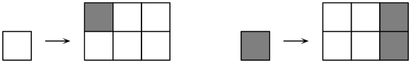
Figure 1. A simple example of a primitive binary block substitution in the plane. It is a stone inflation for the linear map $Q=\operatorname{diag}(3,2)$. The lower left corners of all blocks are used as control points (not shown), which are coloured according to the block type.

Example 7.2.

For the block substitution of Figure 1, the linear expansion is $Q=\operatorname{diag}(3,2)$. With $(z^{\phantom{a}}_{1},z^{\phantom{a}}_{2})=(x,y)$, the polynomials are $p(x,y)=(1+x+x^{2})(1+y)$ together with $q(x,y)=x^{2}(1+y)$, $r(x,y)=y$, $s^{\phantom{a}}_{0}(x,y)=1+x(1+y)$ and $s^{\phantom{a}}_{1}(x,y)=0$. This gives

$$B(k)\,=\,\begin{pmatrix}1+(x+x^{2})(1+y)&(1+x)(1+y)\\ y&x^{2}(1+y)\end{pmatrix}\quad\text{with}\quad(x,y)=\bigl{(}\mathrm{e}^{2\pi\hskip 0.5pt\mathrm{i}\hskip 0.5ptk_{1}},\mathrm{e}^{2\pi\hskip 0.5pt\mathrm{i}\hskip 0.5ptk_{2}}\bigr{)}$$

and $\det\bigl{(}B(k)\bigr{)}=p(x,y)(x^{2}+x^{2}y-y)$. The existence of the various limits of Birkhoff sums we need here, for a.e. $k\in\mathbb{R}^{2}$, follows once again from Lemma 3.7.

The non-zero Lyapunov exponent is given by

$$\begin{split}\mathfrak{m}\hskip 0.5pt(x^{2}+x^{2}y-y)\,&=\,\mathfrak{m}\hskip 0.5pt(x^{2}+x^{2}y+y)\,=\,\mathfrak{m}\hskip 0.5pt(1+x^{-2}y+y)\,=\,\mathfrak{m}\hskip 0.5pt(1+x+y)\\ &=\,\frac{\raisebox{-2.0pt}{$3\sqrt{3}$}}{\raisebox{0.5pt}{$4\hskip 0.5pt\pi$}}\,L(2,\chi^{\phantom{a}}_{-3})\,=\,2\int_{0}^{1/3}\!\log\bigl{(}2\cos(\pi t)\bigr{)}\,\mathrm{d}t\,\approx\,0.323{\hskip 0.5pt}066\hskip 0.5pt,\end{split}$$

where $L(z,\chi^{\phantom{a}}_{-3})$ is the $L$-function for the principal Dirichlet character $\chi^{\phantom{a}}_{-3}$ of the imaginary quadratic field $\mathbb{Q}\bigl{(}\sqrt{-3}\hskip 0.5pt\hskip 0.5pt\bigr{)}$. Here, the first equality follows from a change of variable transformation, while the third emerges by a standard formula from [25]. The connection between logarithmic Mahler measures and special values of $L$-functions is a famous result that first appeared in [58] as the groundstate entropy of the anti-ferromagnetic Ising model on the triangular lattice; see [49, 3] and references therein for more. $\Diamond$

Remark 7.3.

The absence of ac diffraction immediately implies that the spectral measure for the ‘one-point lookup function’ must be singular. As in the one-dimensional case, this implies that the spectral measure is also singular for any function that looks up the level-$n$ supertile at the origin; see the discussion before Corollary 5.1. Then, by [15], any spectral measure must be singular, and our system has singular dynamical spectrum. This gives another, independent proof of a result that was previously shown in [26, 7]; see also [29]. $\Diamond$

8. Block substitutions with squares

Here, we are interested in inflation rules with a single prototile of unit area and linear expansion $Q$, but some added complexity from the set $S$ of relative positions of the tiles within the supertile. In particular, this will be our first class of examples where we go beyond the FLC case. The special interest in this class originates from the fact that the Fourier matrix cocycle, $B^{(n)}(k)$, simply is a sequence of multivariate trigonometric polynomials. We thus write $P^{(n)}(k)$ to indicate this. The renormalisation equation becomes an equation directly for the autocorrelation and reads

(21) $$\gamma\,=\,\nu*(f.\gamma)\quad\text{with}\quad\nu\,=\,\frac{\raisebox{-2.0pt}{$\delta^{\phantom{a}}_{S}*{\delta^{\phantom{a}}_{-S}}$}}{\raisebox{0.5pt}{$\lvert\det(Q)\rvert$}}\hskip 0.5pt.$$

Let us begin with a particularly simple case.

Example 8.1.

The staggered block substitution defined by

with arbitrary $a\in\mathbb{R}$ results in a tiling that is lattice-periodic, with lattice $\varGamma=\langle v,e^{\phantom{a}}_{2}\rangle^{\phantom{a}}_{\mathbb{Z}\hskip 0.5pt}$, where $v=e^{\phantom{a}}_{1}+a\hskip 0.5pte^{\phantom{a}}_{2}$. In particular, the resulting tiling is $1$-periodic in $e^{\phantom{a}}_{2}$-direction. Since $\operatorname{dens}(\varGamma)=1$, the autocorrelation is $\gamma=\delta^{\phantom{a}}_{\varGamma}$, where we use a reference point in the lower left corner of every unit square as indicated. The diffraction measure is $\widehat{\gamma}=\delta^{\phantom{a}}_{\varGamma^{*}}$ with the dual lattice $\varGamma^{*}=\langle e^{\phantom{a}}_{1},e^{\phantom{a}}_{2}-a\hskip 0.5pte^{\phantom{a}}_{1}\rangle^{\phantom{a}}_{\mathbb{Z}\hskip 0.5pt}$.

Let us look at this result from the renormalisation point of view, which is also applicable here because the inflation can easily be changed into a stone inflation without changing the control point positions; see Remark 8.2 below. As mentioned above, the approach also works for periodic cases, like the one at hand. By an iteration of the renormalisation equation (21) and an application of Lemma 2.4, the autocorrelation is

$$\gamma\,=\operatorname*{\text{\Huge\raisebox{-3.5pt}{$\ast$}}}_{m\geqslant 0}f^{m}\!.\hskip 0.5pt\nu\quad\text{with}\quad\nu\,=\,\bigl{(}\delta^{\phantom{a}}_{0}+\tfrac{1}{2}(\delta^{\phantom{a}}_{e^{\phantom{a}}_{2}}+\delta^{\phantom{a}}_{-e^{\phantom{a}}_{2}})\bigr{)}*\bigl{(}\delta^{\phantom{a}}_{0}+\tfrac{1}{2}(\delta^{\phantom{a}}_{v}+\delta^{\phantom{a}}_{-v})\bigr{)},$$

where $f(x)=2\hskip 0.5ptx$. Now, Fourier transform leads to the two-dimensional Riesz product

$$\widehat{\gamma}\,=\prod_{m\geqslant 0}\bigl{(}1+\cos(2\pi\hskip 0.5pt2^{m}(k^{\phantom{a}}_{1}+a\hskip 0.5ptk^{\phantom{a}}_{2}))\bigr{)}\bigl{(}1+\cos(2\pi\hskip 0.5pt2^{m}k^{\phantom{a}}_{2})\bigr{)}\,=\sum_{\ell\in\mathbb{Z}\hskip 0.5pt}\widehat{\gamma}^{(1)}_{\ell}\times\delta^{(2)}_{\ell}$$

with $\widehat{\gamma}^{(1)}_{\ell}\!=\prod_{m\geqslant 0}\bigl{(}1+\cos(2\pi\hskip 0.5pt2^{m}(k^{\phantom{a}}_{1}+a\hskip 0.5pt\ell))\bigr{)}$ and $k=(k^{\phantom{a}}_{1},k^{\phantom{a}}_{2})$. Here, we have adopted the standard notation for product distributions or measures, where the upper index refers to the two coordinate directions. Clearly, one has $\widehat{\gamma}^{(1)}_{0}=\delta^{(1)}_{\mathbb{Z}\hskip 0.5pt}$ by Lemma 2.6. Moreover, the distribution $\widehat{\gamma}^{(1)}_{\ell}$ is $1$-periodic for every $\ell\in\mathbb{Z}\hskip 0.5pt$, which means that $\widehat{\gamma}$ is $1$-periodic in $e^{\phantom{a}}_{1}$-direction, independently of $a$.

Whenever $a\in\mathbb{Z}\hskip 0.5pt$, one finds $\widehat{\gamma}^{(1)}_{\ell}\!=\delta^{(1)}_{\mathbb{Z}\hskip 0.5pt}$ by Lemma 2.6, and hence $\widehat{\gamma}=\delta^{\phantom{a}}_{\mathbb{Z}\hskip 0.5pt^{2}}$ as required. More generally, given $k^{\phantom{a}}_{2}=\ell$, the only contribution to $\widehat{\gamma}^{(1)}_{\ell}$ emerges for $k^{\phantom{a}}_{1}+a\hskip 0.5pt\ell=r\in\mathbb{Z}\hskip 0.5pt$, hence for $k=r\hskip 0.5pte^{\phantom{a}}_{1}+\ell(e^{\phantom{a}}_{2}-a\hskip 0.5pte^{\phantom{a}}_{1})\in\varGamma^{*}$, which means that the Riesz product representation also gives $\widehat{\gamma}=\delta^{\phantom{a}}_{\varGamma^{*}}$, as it must.

Looking at this result from the cocycle point of view gives $P(k)=(1+y)(1+x\hskip 0.5pty^{a})$ with $x=\mathrm{e}^{2\pi\hskip 0.5pt\mathrm{i}\hskip 0.5ptk_{1}}$ and $y=\mathrm{e}^{2\pi\hskip 0.5pt\mathrm{i}\hskip 0.5ptk_{2}}$, so that

$$\chi^{P}(k)\,:=\lim_{n\to\infty}\frac{\raisebox{-2.0pt}{$1$}}{\raisebox{0.5pt}{$n$}}\sum_{\ell=0}^{n-1}\log\lvert P(2^{\ell}k)\rvert\,=\,\mathbb{M}\bigl{(}\log\hskip 0.5pt\lvert P\rvert\bigr{)}$$

holds for a.e. $k\in\mathbb{R}^{2}$ by Lemma 3.8, where one observes that $\log\hskip 0.5pt\lvert P\rvert=\frac{1}{2}\log\hskip 0.5pt\lvert P\rvert^{2}$ with $\lvert P\rvert^{2}$ satisfying the required conditions. Now, the mean can be calculated as

$$\mathbb{M}\bigl{(}\log\hskip 0.5pt\lvert P\rvert\bigr{)}\,=\,\mathfrak{m}\hskip 0.5pt^{\phantom{a}}_{y}(1+y)\,+\lim_{T\to\infty}\frac{\raisebox{-2.0pt}{$1$}}{\raisebox{0.5pt}{$T$}}\int_{0}^{T}\!\mathfrak{m}\hskip 0.5pt^{\phantom{a}}_{x}(1+x\hskip 0.5pty^{a})\,\mathrm{d}k^{\phantom{a}}_{2}\,=\,0\hskip 0.5pt,$$

where both Mahler measures are zero because all roots of the polynomials lie on the unit circle. This fits with the explicit calculation of $\widehat{\gamma}$ from above. $\Diamond$

Remark 8.2.

By standard methods, which are explained in [8] and in [33], one can replace the square in Example 8.1 with a new prototile so that the inflation rule is turned into a stone inflation. This has no effect on the position of the control point, wherefore we continue with the simpler formulation as a block stubstitution.

In the same vein, one can see that our approach also works for more general inflation rules, certainly as long as they are MLD with a stone inflation. For examples of such rules and their reduction to stone inflations, we refer to [8, Ch. 5] and [33]. $\Diamond$

Extending this initial example, we may consider a block substitution with $M$ columns of $N$ blocks each, where entire columns can be shifted in vertical direction by an arbitrary amount, as indicated in the next diagram,

(22)

When using the lower left corner as reference point for each square, it is clear that a modification into a stone inflation according to Remark 8.2 does not change the resulting point set. For this reason, we stick to the formulation with squares for simplicity.

Let us now assume that the $i$th column is shifted by $a_{i}\in\mathbb{R}$ in vertical direction, with $i\in\{0,1,\ldots,M-1\}$. Since $a^{\phantom{a}}_{0}$ only results in a global shift of the entire block, we set $a^{\phantom{a}}_{0}=0$ without loss of generality, and consider the remaining $a_{i}$ as shifts relative to column $0$.

As in the previous case, which had the FLC property, we define the hull as the orbit closure of a fixed point tiling, where the closure is now taken with respect to the local rubber topology [13]. This defines a compact tiling space [30], without any change in the FLC case. However, this slight modification takes care of the potential occurrence of a tiling with infinite local complexity. As before, we obtain a dynamical system, under the continuous translation action of $\mathbb{R}^{2}$, which is uniquely ergodic; see also [41]. Each tiling in the hull is $1$-periodic in the $e^{\phantom{a}}_{2}$-direction.

From the set $S$ of relative displacements, one finds

$$P(k)\,=\,\overline{\widehat{\delta^{\phantom{a}}_{S}}}(k)\,=\,(1+y+\ldots+y^{N-1})\bigl{(}1+xy^{a^{\phantom{a}}_{1}}+x^{2}y^{a^{\phantom{a}}_{2}}+\ldots+x^{M-1}y^{a^{\phantom{a}}_{M-1}}\bigr{)}$$

with $x=\mathrm{e}^{2\pi\hskip 0.5pt\mathrm{i}\hskip 0.5ptk_{1}}$ and $y=\mathrm{e}^{2\pi\hskip 0.5pt\mathrm{i}\hskip 0.5ptk_{2}}$. Note that the trigonometric polynomial $P$ is quasiperiodic, but $1$-periodic in $k_{1}$. Now, with $Q=\operatorname{diag}(M,N)$, the cocycle is defined by

$$P^{(n)}(k)\,=\,P(k)\hskip 0.5ptP(Qk)\cdots P(Q^{n-1}k)\hskip 0.5pt,$$

with $P^{(1)}=P$ as usual. Our Lyapunov exponent can be calculated as follows,

$$\chi^{P}(k)\,=\lim_{n\to\infty}\frac{\raisebox{-2.0pt}{$1$}}{\raisebox{0.5pt}{$n$}}\log\big{|}P^{(n)}(k)\big{|}\,=\lim_{n\to\infty}\frac{\raisebox{-2.0pt}{$1$}}{\raisebox{0.5pt}{$n$}}\sum_{\ell=0}^{n-1}\log\big{|}P(Q^{\ell}k)\big{|}.$$

By an obvious variant of Lemma 3.8, where $\alpha$ is replaced by the expansion $Q$, the limit exists for a.e. $k\in\mathbb{R}^{2}$ and is given by

$$\begin{split}\mathbb{M}\bigl{(}\log\hskip 0.5pt\lvert P\rvert\bigr{)}\,&=\lim_{T\to\infty}\frac{\raisebox{-2.0pt}{$1$}}{\raisebox{0.5pt}{$T$}}\int_{0}^{T}\int_{0}^{1}\log\big{|}P(k)\big{|}\,\mathrm{d}k^{\phantom{a}}_{1}\,\mathrm{d}k^{\phantom{a}}_{2}\\ &=\mathfrak{m}\hskip 0.5pt^{\phantom{a}}_{y}\bigl{(}1+y+\ldots+y^{N-1}\bigr{)}\,+\lim_{T\to\infty}\frac{\raisebox{-2.0pt}{$1$}}{\raisebox{0.5pt}{$T$}}\int_{0}^{T}\!\mathfrak{m}\hskip 0.5pt^{\phantom{a}}_{x}\bigl{(}1+xy^{a^{\phantom{a}}_{1}}+\ldots+x^{M-1}y^{a^{\phantom{a}}_{M-1}}\bigr{)}\,\mathrm{d}k^{\phantom{a}}_{2}\hskip 0.5pt.\end{split}$$

As $1+y+\ldots+y^{N-1}$ is cyclotomic, the first term vanishes. The integrand in the second is the logarithmic Mahler measure of a polynomial (in $x$) with all coefficients on the unit circle, which is known as a unimodular polynomial. By an application of Jensen’s inequality in conjunction with Parseval’s equation, one can show that its logarithmic Mahler measure is bounded by $\log\sqrt{M}$ for every $k^{\phantom{a}}_{2}\in\mathbb{R}$. Consequently, we have

$$\mathbb{M}\bigl{(}\log\hskip 0.5pt\lvert P\rvert\bigr{)}\,\leqslant\,\log\sqrt{M}\,<\,\log\sqrt{MN}$$

because $N>1$ by assumption. This implies that we cannot have any absolutely continuous diffraction, and $\widehat{\gamma}$ must be singular.

The remarkable aspect of this simple class of examples is that the tilings are generally not FLC; compare [33] and references therein. One can say a bit more about the explicit structure of the diffraction measure. First of all, it is $1$-periodic in $e^{\phantom{a}}_{1}$-direction, and it consists of parallel arrangements of one-dimensional layers, distinct in general, which have their own Riesz product representation. We leave further details to the interested reader.

Remark 8.3.

The above results can be generalised to $\mathbb{R}^{d+1}$ with $d\geqslant 1$ as follows. Consider a block of $M^{\phantom{a}}_{1}\times\cdots\times M^{\phantom{a}}_{d}\times N$ cubes, with each $M_{i}\geqslant 2$ and $N\geqslant 2$. Now, modify this block as an arrangement of $M^{\phantom{a}}_{1}\times\cdots\times M^{\phantom{a}}_{d}$ columns of $N$ cubes each, where column $(m^{\phantom{a}}_{1},\ldots,m^{\phantom{a}}_{d})$ is shifted by an arbitrary real number $a^{\phantom{a}}_{m^{\phantom{a}}_{1},\ldots,m^{\phantom{a}}_{d}}$ in $e^{\phantom{a}}_{d+1}$-direction. We may set $a^{\phantom{a}}_{0,\ldots,0}=0$ without loss of generality. With $Q=\operatorname{diag}(M^{\phantom{a}}_{1},\ldots,M^{\phantom{a}}_{d},N)$, one can now repeat the above analysis. Here, one obtains tilings of $\mathbb{R}^{d+1}$ that are $1$-periodic in $e^{\phantom{a}}_{d+1}$-direction.

Writing $z=(z^{\phantom{a}}_{1},\ldots,z^{\phantom{a}}_{d},z^{\phantom{a}}_{d+1})=\bigl{(}\mathrm{e}^{2\pi\hskip 0.5pt\mathrm{i}\hskip 0.5ptk_{1}},\ldots,\mathrm{e}^{2\pi\hskip 0.5pt\mathrm{i}\hskip 0.5ptk_{d}},\mathrm{e}^{2\pi\hskip 0.5pt\mathrm{i}\hskip 0.5ptk_{d+1}}\bigr{)}=(x^{\phantom{a}}_{1},\ldots,x^{\phantom{a}}_{d},y)$, one finds

$$\begin{split}P(k)\,&=\,\bigl{(}1+y+\ldots+y^{N-1}\bigr{)}R(k)\quad\text{with}\\[2.84526pt] R(k)\,&=\sum_{m^{\phantom{a}}_{1}=0}^{M_{1}-1}\cdots\sum_{m^{\phantom{a}}_{d}=0}^{M_{d}-1}x^{m_{1}}_{1}\cdots\hskip 0.5ptx^{m_{d}}_{d}\,y^{a^{\phantom{a}}_{m_{1},\ldots,m_{d}}},\end{split}$$

where $R$, and hence also $P$, is $1$-periodic in $e_{i}$-direction for all $1\leqslant i\leqslant d$. The maximal Lyapunov exponent, for a.e. $k\in\mathbb{R}^{d+1}$, is now given by

$$\begin{split}\chi^{B}(k)\,&=\lim_{T\to\infty}\frac{\raisebox{-2.0pt}{$1$}}{\raisebox{0.5pt}{$T$}}\int_{0}^{T}\!\mathfrak{m}\hskip 0.5pt^{\phantom{a}}_{x}(R)\,\mathrm{d}k^{\phantom{a}}_{d+1}\,\leqslant\,\log\sqrt{M_{1}\cdots M_{d}\,}\\[2.84526pt] &=\,\frac{\raisebox{-2.0pt}{$1$}}{\raisebox{0.5pt}{$2$}}\sum_{i=1}^{d}\log(M_{i})\,<\,\frac{\raisebox{-2.0pt}{$1$}}{\raisebox{0.5pt}{$2$}}\log\bigl{(}\det(Q)\bigr{)},\end{split}$$

where the last estimate is a consequence of $N\geqslant 2$, while the intermediate steps work in complete analogy to our above treatment for $d=1$. The conclusion is, once again, the absence of absolutely continuous diffraction. $\Diamond$

Obviously, one can extend this class of examples by colouring blocks. This will lead to higher-dimensional Fourier matrices again, with an uncoloured tiling of the above type as a factor system. We leave further details to the interested reader, and turn to a perhaps more interesting non-FLC example.

9. The Frank–Robinson tiling

Let us take a closer look at the tiling dynamical system defined by the stone inflation

(23)

where the short edge has length $1$ and the long one length $\lambda=\frac{1}{2}\bigl{(}1+\sqrt{13}\,\bigr{)}\approx 2.303$, while the linear expansion is $Q=\lambda\hskip 0.5pt\mathbbm{1}^{\phantom{a}}_{2}$. This inflation defines the Frank–Robinson tiling [30], see also [27], a patch of which is shown in Figure 2. Note that the algebraic integer $\lambda$ is neither a PV number nor a unit. By standard PF theory, the relative prototile frequencies in any Frank–Robinson tiling are given by

(24) $$(\nu^{\phantom{a}}_{1},\ldots,\nu^{\phantom{a}}_{4})\,=\,\frac{\raisebox{-2.0pt}{$1$}}{\raisebox{0.5pt}{$9$}}(4-\lambda,4\lambda-7,4\lambda-7,19-7\lambda)\hskip 0.5pt;$$

see [8, Ex. 5.8] for details. With the chosen edge lengths, the density of the control point set $\varLambda$ induced by Eq. (23) is $\operatorname{dens}(\varLambda)=(3+\lambda)/13\approx 0.408$.

Figure 2. A patch of the Frank–Robinson tiling defined by the stone inflation rule (23), obtained by three inflation steps from a single large square.

If we define the hull as the orbit closure of a fixed point tiling (under the square of the rule (23)) in the local rubber topology, we get a compact tiling space of infinite local complexity; see [30] and [8, Ex. 5.8] for more. As in the FLC case, it is also true here [41, Cor. 5.7 and Ex. 6.3] that the tiling dynamical system does not have any non-trivial eigenfunction. In the diffraction context, this implies that the pp part consists of the trivial Bragg peak at $k=0$ only; see below for its intensity.

By taking the lower-left corner of each prototile as its control point, as indicated in Eq. (23) and Figure 2, we turn each tiling of the hull into a Delone set that is MLD with the tiling. Now, the absence of non-trivial eigenfunctions translates to the diffraction of this Delone set by asserting that the trivial Bragg peak at $k=0$ is the only contribution to the pure point part of the diffraction measure.

The Fourier matrix $B$ is given by

(25) $$B(x,y)\,=\,\begin{pmatrix}x^{2}\hskip 0.5pty^{2}&1&1&1\\ p(x,y)&0&r(y)&0\\ p(y,x)&r(x)&0&0\\ q(x,y)&0&0&0\end{pmatrix},\qquad\text{with }(x,y)=\bigl{(}\mathrm{e}^{2\pi\hskip 0.5pt\mathrm{i}\hskip 0.5ptk_{1}},\mathrm{e}^{2\pi\hskip 0.5pt\mathrm{i}\hskip 0.5ptk_{2}}\bigr{)}$$

and the (trigonometric) polynomials

(26) $$\begin{split}r(x)\,&=\,x^{\lambda}+x^{\lambda+1}+x^{\lambda+2},\\ p(x,y)\,&=\,x^{2}+x^{2}\hskip 0.5pty+y^{\lambda+2},\\ q(x,y)\,&=\,1+x+y+x\hskip 0.5pty+x^{\lambda}y^{\lambda}\bigl{(}x^{2}+y^{2}+x\hskip 0.5pty^{2}+x^{2}y+x^{2}y^{2}\bigr{)}.\end{split}$$

Note that $B(0)$ is the inflation matrix of the tiling, with PF eigenvalue $\lambda^{2}$.

Now, the cocycle is given by $B^{(n)}(k)=B(k)B(\lambda k)\cdots B(\lambda^{n-1}k)$, with maximal Lyapunov exponent

$$\chi^{B}(k)\,=\,\limsup_{n\to\infty}\frac{\raisebox{-2.0pt}{$1$}}{\raisebox{0.5pt}{$n$}}\log\|B^{(n)}(k)\|\hskip 0.5pt,$$

where the choice of the (sub-multiplicative) matrix norm is arbitrary. Absence of absolutely continuous diffraction will be implied if we show that $\chi^{B}(k)\leqslant\log(\lambda)-\varepsilon$ for some $\varepsilon>0$ and a.e. $k\in\mathbb{R}^{2}$. Since it is convenient to work with the square of the Frobenius norm, we prefer to compare $2\hskip 0.5pt\hskip 0.5pt\chi^{B}$ with $\log(\lambda^{2})\approx 1.668$ instead.

By standard subadditive arguments along the lines used for our previous examples, one finds that, for any $N\in\mathbb{N}$ and then a.e. $k\in\mathbb{R}^{2}$,

(27) $$2\hskip 0.5pt\hskip 0.5pt\chi^{B}(k)\,\leqslant\,\frac{\raisebox{-2.0pt}{$1$}}{\raisebox{0.5pt}{$N$}}\,\mathbb{M}\bigl{(}\log\|B^{(N)}(.)\|^{2}_{\mathrm{F}}\bigr{)}\,=:\,\mathfrak{m}\hskip 0.5pt^{\phantom{a}}_{N}\hskip 0.5pt,$$

where $\mathbb{M}$ again denotes the mean. Since $\log\|B^{(N)}(.)\|^{2}_{\mathrm{F}}$ is a quasiperiodic function in two variables, with fundamental frequencies $1$ and $\lambda$, the mean can be expressed as an integral over the $4$-torus, $\mathbb{T}^{4}$. To this end, one introduces new variables $u^{\phantom{a}}_{1},u^{\phantom{a}}_{2}$ and $v^{\phantom{a}}_{1},v^{\phantom{a}}_{2}$ such that

$$B(k)\,=\,\tilde{B}(u^{\phantom{a}}_{1},u^{\phantom{a}}_{2},v^{\phantom{a}}_{1},v^{\phantom{a}}_{2})\big{|}_{u^{\phantom{a}}_{1}=\lambda k^{\phantom{a}}_{1}\hskip 0.5pt,\,u^{\phantom{a}}_{2}=k^{\phantom{a}}_{1}\hskip 0.5pt,\,v^{\phantom{a}}_{1}=\lambda k^{\phantom{a}}_{2}\hskip 0.5pt,\,v^{\phantom{a}}_{2}=k^{\phantom{a}}_{2}}$$

where $\tilde{B}$ is $1$-periodic in each variable. Here, $\tilde{B}$ is defined in complete analogy to (25), with the corresponding modifications on $r$, $p$ and $q$ from Eq. (26); compare [4] for a related one-dimensional case analysed previously. One now finds

(28) $$\mathfrak{m}\hskip 0.5pt^{\phantom{a}}_{N}\,=\,\frac{\raisebox{-2.0pt}{$1$}}{\raisebox{0.5pt}{$N$}}\,\mathbb{M}\bigl{(}\log\|\tilde{B}^{(N)}(.)\|^{2}_{\mathrm{F}}\bigr{)}\,=\,\frac{\raisebox{-2.0pt}{$1$}}{\raisebox{0.5pt}{$N$}}\int_{\mathbb{T}^{4}}\log\|\tilde{B}^{(N)}(u^{\phantom{a}}_{1},u^{\phantom{a}}_{2},v^{\phantom{a}}_{2},v^{\phantom{a}}_{2})\|^{2}_{\mathrm{F}}\,\mathrm{d}u^{\phantom{a}}_{1}\,\mathrm{d}u^{\phantom{a}}_{2}\,\mathrm{d}v^{\phantom{a}}_{1}\,\mathrm{d}v^{\phantom{a}}_{2}\hskip 0.5pt,$$

which can be calculated numerically with good precision. Figure 3 illustrates the result.

Figure 3. Numerical values of the upper bounds $\mathfrak{m}\hskip 0.5pt^{\phantom{a}}_{N}$ of $2\hskip 0.5pt\chi^{B}$ from Eq. (28), for $1\leqslant n\leqslant 10$. The horizontal line is at height $2\log(\lambda)\approx 1.668$. The estimated numerical errors are indicated by vertical bars (the dotted line is for eye guidance only).

Let us summarise this section as follows.

Theorem 9.1.

Let $\varLambda$ be the set of control points of any element of the Frank–Robinson tiling hull. Then, the diffraction measure of the corresponding Dirac comb, $\delta^{\phantom{a}}_{\!\varLambda}$, is of the form $\widehat{\gamma}=\operatorname{dens}(\varLambda)^{2}\,\delta^{\phantom{a}}_{0}+\widehat{\gamma}^{\phantom{a}}_{\mathsf{sc}}$, where the singular continuous part can be expressed in terms of a generalised Riesz product.

More generally, if one assigns general complex weights $u^{\phantom{a}}_{1},\ldots,u^{\phantom{a}}_{4}$ to the four types of control points, not all zero, the corresponding diffraction measure is still singular, where the only point measure is the central peak at $0$ with intensity

$$I_{0}\,=\,\operatorname{dens}(\varLambda)^{2}\,\big{|}\nu^{\phantom{a}}_{1}u^{\phantom{a}}_{1}+\ldots+\nu^{\phantom{a}}_{4}u^{\phantom{a}}_{4}\big{|}^{2},$$

where $\operatorname{dens}(\varLambda)=(3+\lambda)/13$ and the $\nu^{\phantom{a}}_{i}$ are the prototile frequencies from Eq. (24). ∎

The natural next step consists in defining the (integrated) distribution function for $\widehat{\gamma}^{\phantom{a}}_{\mathsf{sc}}$ in the positive quadrant, as

$$F(k^{\phantom{a}}_{1},k^{\phantom{a}}_{2})\,=\,\widehat{\gamma}^{\phantom{a}}_{\mathsf{sc}}\bigl{(}[0,k^{\phantom{a}}_{1}]\!\times\![0,k^{\phantom{a}}_{2}]\bigr{)},$$

with the matching extension to the other quadrants. This leads to a continuous function (which requires an extra argument along the directions of $e^{\phantom{a}}_{1}$ and $e^{\phantom{a}}_{2}$; compare [7, Sec. 5] for a similar analysis) which behaves as $F(k^{\phantom{a}}_{1},k^{\phantom{a}}_{2})\sim\gamma(\{0\})\,k^{\phantom{a}}_{1}k^{\phantom{a}}_{2}$ for large values of $k^{\phantom{a}}_{1}$ and $k^{\phantom{a}}_{2}$. As such, it does not reveal the interesting structure of the sc measure. A better understanding of the latter requires a multi-fractal analysis, which is outside the scope of this survey.

At this point, it is suggestive to assume that also the dynamical spectrum is singular, in particular in the light of [14], but we have no complete answer to this question at present.

10. Closing remarks

As we have illustrated by various examples, Lyapunov exponents lead to useful insight on the spectral nature of inflation tilings in any dimension. They are a powerful tool to exclude absolutely continuous spectral components. So far, our approach is taylored to inflation tiling spaces with finitely many prototiles up to translations, and thus gives no new insight to pinwheel-type systems. Nevertheless, the latter also have a strong renormalisation structure, and further progress seems possible.

To explore the absence of ac diffraction and spectral measures in more generality, one would need a more analytic (rather than numerical) approach to the estimates for upper bounds, or, ideally, exact expressions of Fürstenberg type for the exponents. Also, it would help to establish the almost sure existence of Lyapunov exponents as limits, which does not seem to be an easy task outside the constant-length or the Pisot case.

In this exposition, we have mainly considered the absolutely continuous part of the spectrum. It is not difficult to analyse the pure point part as well, where some results are discussed in [5, 6]. Considerably more involved seems the singular continuous part, which originates from the different scalings one encounters. Various results on the spectral measures in one dimension are derived in [18, 19] via matrix Riesz products, which are not restricted to the self-similar case. It would be interesting to establish a connection with the topological constraints on size and shape changes [21, 22], which should at least be possible in the irreducible Pisot case.

References

- [1] Akiyama S, Barge M, Berthé V, Lee J-Y and Siegel A, On the Pisot substitution conjecture, in [38], pp. 33–72.
- [2] Aubry S, Godrèche C and Luck J M, Scaling properties of a structure intermediate between quasiperiodic and random, J. Stat. Phys. 51 (1988) 1033–1074.
- [3] Baake M, Coons M and Mañibo N, Binary constant-length substitutions and Mahler measures of Borwein polynomials, in From Analysis to Visualization, Bailey D H, Borwein N S, Brent R P, Burachik J H, Osborn J H, Sims B and Zhu Q J (eds.), Springer, Cham (2020), pp. 303–322; arXiv:1711.02492.
- [4] Baake M, Frank N P, Grimm U and Robinson E A, Geometric properties of a binary non-Pisot inflation and absence of absolutely continuous diffraction, Studia Math. 247 (2019) 109–154; arXiv:1706.03976.
- [5] Baake M and Gähler F, Pair correlations of aperiodic inflation rules via renormalisation: Some interesting examples, Topol. & Appl. 205 (2016) 4–27; arXiv:1511.00885.
- [6] Baake M, Gähler F and Mañibo N, Renormalisation of pair correlation measures for primitive inflation rules and absence of absolutely continuous diffraction, Commun. Math. Phys. 370 (2019) 591–635; arXiv:1805.09650.
- [7] Baake M and Grimm U, Squirals and beyond: Substitution tilings with singular continuous spectrum, Ergodic Th. & Dynam. Syst. 34 (2014) 1077–1102; arXiv:1205.1384.
- [8] Baake M and Grimm U, Aperiodic Order. Vol. : A Mathematical Invitation, Cambridge University Press, Cambridge (2013).
- [9] Baake M and Grimm U (eds.), Aperiodic Order. Vol. : Crystallography and Almost Periodicity, Cambridge University Press, Cambridge (2017).
- [10] Baake M, Grimm U and Mañibo N, Spectral analysis of a family of binary inflations rules, Lett. Math. Phys. 108 (2018) 1783–1805; arXiv:1709.09083.
- [11] Baake M, Haynes A and Lenz D, Averaging almost periodic functions along exponential sequences, in [9], pp. 343–362; arXiv:1704.08120.
- [12] Baake M and Lenz D, Dynamical systems on translation bounded measures: Pure point dynamical and diffraction spectra, Ergodic Th. & Dynam. Syst. 24 (2004) 1867–1893; arXiv:math.DS/0302061.
- [13] Baake M and Lenz D, Spectral notions of aperiodic order, Discr. Cont. Dynam. Syst. S 10 (2017) 161–190; arXiv:1601.06629.
- [14] Baake M, Lenz D and van Enter A C D, Dynamical versus diffraction spectrum for structures with finite local complexity, Ergodic Th. & Dynam. Syst. 35 (2015) 2017–2043; arXiv:1307.7518.
- [15] Bartlett A, Spectral theory of substitutions, Ergodic Th. & Dynam. Syst. 38 (2018) 1289–1341; arXiv:1410.8106.
- [16] Berg C and Forst G, Potential Theory on Locally Compact Abelian Groups, Springer, Berlin (1975).
- [17] Berlinkov A and Solomyak B, Singular substitutions of constant length, Ergodic Th. & Dynam. Syst. 39 (2019) 2384–2402; arXiv:1705.00899.
- [18] Bufetov A and Solomyak B, On the modulus of continuity for spectral measures in substitution dynamics, Adv. Math. 260 (2014) 84–129; arXiv:1305.7373.
- [19] Bufetov A and Solomyak B, A spectral cocycle for substitution systems and translation flows, J. Anal. Math. (in press); arXiv:1802.04783.
- [20] Chan L and Grimm U, Spectrum of a Rudin–Shapiro-like sequence, Adv. Appl. Math. 87 (2017) 16–23; arXiv:1611.04446.
- [21] Clark A and Sadun L, When size matters: Subshifts and their related tiling spaces, Ergodic Th. & Dynam. Syst. 23 (2003) 1043–1057; arXiv:math.DE/0201152.
- [22] Clark A and Sadun L, When shape matters: Deformation of tiling spaces, Ergodic Th. & Dynam. Syst. 26 (2006) 69–86; arXiv:math.DE/0306214.
- [23] Corduneanu C, Almost Periodic Functions, 2nd English ed. (Chelsea, New York, 1989).
- [24] Einsiedler M and Ward T, Ergodic Theory — with a View Towards Number Theory, Springer, London (2011).
- [25] Everest G and Ward T, Heights of Polynomials and Entropy in Algebraic Dynamics, Springer, London (1999).
- [26] Frank N P, Multi-dimensional constant-length substitution sequences, Topol. & Appl. 152 (2005) 44–69.
- [27] Frank N P, A primer of substitution tilings of the Euclidean plane, Expo. Math. 26 (2008) 295–326; arXiv:0705.1142.
- [28] Frank N P, Tilings with infinite local complexity, in [38], pp. 223–257; arXiv:1312.4987.
- [29] Frank N P, Introduction to hierarchical tiling dynamical systems, in Tiling and Discrete Geometry (this volume), Akiyama S and Arnoux P (eds.), Springer, Berlin (2020); arXiv:1802.09956.
- [30] Frank N P and Robinson E A, Generalized -expansions, substitution tilings, and local finiteness, Trans. Amer. Math. Soc. 360 (2008) 1163–1177; arXiv:math.DS/0506098.
- [31] Frank N P and Sadun L, Topology of (some) tiling spaces without finite local complexity, Discr. Cont. Dynam. Syst. A 23 (2009) 847–865; arXiv:math.DS/0701424.
- [32] Frank N P and Sadun L, Fusion: A general framework for hierarchical tilings of , Geom. Dedicata 171 (2014) 149–186; arXiv:1101.4930.
- [33] Frettlöh D, More inflation tilings, in [9], pp. 1–37.
- [34] Frettlöh D and Richard C, Dynamical properties of almost repetitive Delone sets, Discr. Cont. Dynam. Syst. A 34 (2014) 531–556; arXiv:1210.2955.
- [35] Godrèche C and Luck J M, Multifractal analysis in reciprocal space and the nature of the Fourier transform of self-similar structures, J. Phys. A: Math. Gen. 23 (1990) 3769–3797.
- [36] Halmos P R, Measure Theory, reprint, Springer, New York (1974).
- [37] Hartinger J, Kainhofer R F and Tichy R F, Quasi-Monte Carlo algorithms for unbounded, weighted integration problems, J. Complexity 20 (2004) 654–668.
- [38] Kellendonk J, Lenz D and Savinien J (eds.), Mathematics of Aperiodic Order, Birkhäuser, Basel (2015).
- [39] Kuipers L and Niederreiter H, Uniform Distribution of Sequences, reprint, Dover, New York (2006).
- [40] Lee J-Y, Moody R V and Solomyak B, Pure point dynamical and diffraction spectra, Ann. H. Poincaré 3 (2002) 1003–1018; arXiv:0910.4809.
- [41] Lee J-Y and Solomyak B, On substitution tilings and Delone sets without finite local complexity, Discr. Cont. Dynam. Syst. A 39 (2019) 3149–3177; arXiv:1804.10235.
- [42] Lieb E H and Loss M, Analysis, 2nd ed., American Mathematical Society, Providence, RI (2001).
- [43] Luck J M, A classification of critical phenomena on quasi-crystals and other aperiodic structures, Europhys. Lett. 24 (1993) 359–364.
- [44] Mañibo N, Lyapunov exponents for binary substitutions of constant length, J. Math. Phys. 58 (2017) 113504 (9 pp); arXiv:1706.00451.
- [45] Mañibo N, Spectral analysis of primitive inflation rules, Oberwolfach Rep. 14 (2017) 2830–2832.
- [46] Moody R V and Strungaru N, Almost periodic measures and their Fourier transforms, in [9], pp. 173–270.
- [47] Peres Y, Schlag W and Solomyak B, Sixty years of Bernoulli convolutions, in Fractal Geometry and Stochastics II, Bandt C, Graf S and Zähle M (eds.), Birkhäuser, Basel (2000), pp. 39–65.
- [48] Queffélec M, Substitution Dynamical Systems — Spectral Analysis, 2nd ed., LNM 1294, Springer, Berlin (2010).
- [49] Schmidt K, Dynamical Systems of Algebraic Origin, Birkhäuser, Basel (1995).
- [50] Simon B, Analysis, Part I: Real Analysis, AMS, Providence, RI (2014).
- [51] Sing B, Pisot Substitutions and Beyond, PhD thesis, Bielefeld University (2007). Available electronically at urn:nbn:de:hbz:361-11555.
- [52] Sobol I M, Calculation of improper integrals using uniformly distributed sequences, Soviet Math. Dokl. 14 (1973) 734–738.
- [53] Solomyak B, Nonperiodicity implies unique composition for self-similar translationally finite tilings, Discr. Comput. Geom. 20 (1989) 265–279.
- [54] Solomyak B, Dynamics of self-similar tilings, Ergodic Th. & Dynam. Syst. 17 (1997) 695–738 and 19 (1999) 1685 (Erratum).
- [55] Solomyak B, Delone sets and dynamical systems, in Tiling and Discrete Geometry (this volume), Akiyama S, Arnoux P (eds.), Springer, Berlin (2020).
- [56] Strungaru N, Almost periodic pure point measures, in [9], pp. 271–342; arXiv:1501.00945.
- [57] Viana M, Lectures on Lyapunov Exponents, Cambridge University Press, Cambridge (2013).
- [58] Wannier G H, Antiferromagnetism. The triangular Ising net, Phys. Rev. 79 (1950) 357–364 and Phys. Rev. B 7 (1973) 5017 (Erratum).