Analysis and synthesis of feature map for kernel-based quantum classifier

Abstract

A method for analyzing the feature map for the kernel-based quantum classifier is developed; that is, we give a general formula for computing a lower bound of the exact training accuracy, which helps us to see whether the selected feature map is suitable for linearly separating the dataset. We show a proof of concept demonstration of this method for a class of 2-qubit classifier, with several 2-dimensional dataset. Also, a synthesis method, that combines different kernels to construct a better-performing feature map in a lager feature space, is presented.

1 Introduction

Over the last 20 years, the unprecedented improvements in the cost-effectiveness ration of computer, together with improved computational techniques, make machine learning widely applicable in every aspect of our lives such as education, healthcare, games, finance, transportation, energy, business, science and engineering HastieTF09 ; Alpaydin16 . Among numerous developed machine learning methods, Support Vector Machine (SVM) is a very established one which has become an overwhelmingly popular choice for data analysis Boser1992 . In SVM method, a nonlinear dataset is transformed via a feature map to another dataset and is separated by a hyperplane in the feature space, which can be effectively performed using the kernel trick. In particular, the Gaussian kernel is often used.

Quantum computing is expected to speed-up the performance of machine learning through exploiting quantum mechanical properties including superposition, interference, and entanglement. As for the quantum classifier, a renaissance began in the past few years, with the quantum SVM method Rebentrost2014 , the quantum circuit learning method Mitarai2018 , and some parallel development by other research groups Neven 2018 ; Zhuang Zhang 2019 ; Wilson2018 . In particular, the kernel method can be exploited as a powerful mean that can be introduced in the quantum SVM as in the classical case Rebentrost2014 ; Chatterjee 2017 ; Bishwas2018 ; LiTongyang2019 ; havlivcek2019 ; Schuld2019 ; Nori 2019 ; Park Rhee 2019 ; Negoro 2019 ; Lloyd2020 ; LaRose2020 ; importantly, the concept of kernel-based quantum classifier has been experimentally demonstrated on a real device havlivcek2019 ; Park Rhee 2019 ; Negoro 2019 . These studies show the possibility that machine learning will get a further boost by using quantum computers in the near future.

For all the developed quantum classification methods, the feature map plays a role to encode the dataset taken from its original low dimensional real space onto a high dimensional quantum state space (i.e., the Hilbert space). A possible advantage of quantum classifier lies in the fact that this high-dimensional feature space is realized on a physical quantum computer even with a medium number of qubits, as well as the fact that the kernel could be computed faster than the classical case. However, in the framework of using gate-based quantum computers, a suitable feature map has to be explicitly specified, which is of course less trivial than specifying a suitable kernel. (Note that a kernel induces a feature map through the reproducing kernel Hilbert space.) Actually, for choosing a suitable feature map, one could prepare many map candidates and try to find a best one by comparing the results of training accuracy attained with all those maps, but this clearly needs numerous times of classification or regression analysis. Hence it is desirable if we have a method for easily having a rough estimate of the training accuracy of every feature map candidate.

This paper gives one such method, based on the minimum accuracy, a lower bound of the exact training accuracy attained by any optimized classifier. The minimum accuracy is determined only from a chosen feature map and the input classical dataset, hence it can be used to screen a library of suitable feature maps. A critical drawback of this method is that it needs calculation of the order of the dimension of the feature space, which is exponential to the number of qubits. Hence, to show the proof of concept, in this paper we study the case where the quantum classifier is composed of only two qubits (see Section 4 for a possible extension of the method). This simple setup gives us an explicit form of the feature map and further a visualization of the encoded input data distribution in the feature space; this eventually enables us to easily calculate the minimum accuracy. Moreover, the visualized feature map candidates might be exploited for combining them to construct a better-performing feature map and accordingly a better kernel. Although the concept of these synthesizing tools is device-independent, in this paper we demonstrate the idea in the framework of havlivcek2019 , with a special type of five encoding functions and four 2-dimensional nonlinear datasets.

2 Methods

2.1 Real-vector representation of the feature map via Pauli decomposition

In the SVM method with quantum kernel estimator, the feature map transforms an input dataset to a set of multi-qubit states, which forms the feature space (i.e., Hilbert space); then the kernel matrix is constructed by calculating all the inner products of quantum states, and it is finally used in the (standard) SVM for classifying the dataset. Surely different feature maps lead to different kernels and accordingly influence on the classification accuracy, meaning that a careful analysis of the feature space is necessary. However, due to the complicated structure of the feature space, such analysis is in general not straightforward. Here, we propose the Pauli-decomposition method for visualizing the feature space, which might be used as a guide to select a suitable feature map.

We begin with a brief summary of the kernel-based quantum SVM method proposed in havlivcek2019 . First, a $\tilde{n}$-dimensional classical data $\bm{x}\in\mathbb{R}^{\tilde{n}}$ is encoded into the unitary operator $\mathcal{U}_{\Phi(\bm{x})}$ through an encoding function ${\Phi(\bm{x})}$, and it is applied to the initial state $\ket{0}^{\otimes n}$ with $\ket{0}$ the qubit ground state. Thus, the feature map is a transformation from the classical data $\bm{x}$ to the quantum state $\ket{\Phi(\bm{x})}=\mathcal{U}_{\Phi(\bm{x})}\ket{0}^{\otimes n}$, and the feature space is $(\mathbb{C}^{2})^{\otimes n}=\mathbb{C}^{2^{n}}$. The kernel is then naturally defined as $K(\bm{x},\bm{z})=|\braket{\Phi(\bm{x})}{\Phi(\bm{z})}|^{2}$; this quantity can be practically calculated as the ratio of zero strings $0^{n}$ in the $Z$-basis measurement result, for the state $\mathcal{U}^{\dagger}_{\Phi(\bm{x})}\mathcal{U}_{\Phi(\bm{z})}\ket{0}^{\otimes n}$. Finally, the constructed kernel is used in the standard manner in SVM; that is, a test data $\bm{x}$ is classified into two categories depending on the sign of

$$\sum_{i=1}^{N}\alpha_{i}y_{i}K(\bm{x}_{i},\bm{x})+b,$$ (1)

where $(\bm{x}_{i},y_{i})~{}(i=1,\ldots,N)$ are the pairs of training data, and $(\alpha_{i},b)$ are the optimized parameters.

Now we introduce the real-vector representation of the feature map. The key idea is simply to use the fact that the kernel can be expressed in terms of the density operator $\rho(x)=\ket{\Phi(\bm{x})}\bra{\Phi(\bm{x})}$ as

$$K(\bm{x},\bm{z})=|\braket{\Phi(\bm{x})}{\Phi(\bm{z})}|^{2}=\mathrm{tr}\left[\rho(\bm{x})\rho(\bm{z})\right],$$ (2)

and the density operator can be always expanded by the set of Pauli operators as

$$\rho(\bm{x})=\sum_{i=1}^{4^{n}}a_{i}(\bm{x})\sigma_{i}$$ (3)

with $a_{i}(\bm{x})\in\mathbb{R}$ and $\sigma_{i}\in P_{n}=\{I,X,Y,Z\}^{\otimes n}$ the multi-qubit Pauli operators. The followings are examples of the elements of $P_{2}$:

$$\begin{split}XI&=\left[\begin{array}[]{rr}0&1\\ 1&0\\ \end{array}\right]\otimes\left[\begin{array}[]{rr}1&0\\ 0&1\\ \end{array}\right],~{}~{}ZY=\left[\begin{array}[]{rr}1&0\\ 0&-1\\ \end{array}\right]\otimes\left[\begin{array}[]{rr}0&-i\\ i&0\\ \end{array}\right],~{}~{}\\ YZ&=\left[\begin{array}[]{rr}0&-i\\ i&0\\ \end{array}\right]\otimes\left[\begin{array}[]{rr}1&0\\ 0&-1\\ \end{array}\right].\end{split}$$

Then, by substituting Eq. (3) into Eq. (2) and using the trace relation $\mathrm{tr}\left(\sigma_{i}\sigma_{j}\right)=2^{n}\delta_{i,j}$, the kernel can be written as

$$K(\bm{x},\bm{z})=2^{n}\sum_{i=1}^{4^{n}}a_{i}(\bm{x})a_{i}(\bm{z}),$$ (4)

meaning that the vector $\bm{a}(\bm{x})=[a_{1}(\bm{x}),\ldots,a_{4^{n}}(\bm{x})]^{\top}$ serves as the feature map corresponding to the kernel $K(\bm{x},\bm{z})$. That is, the input dataset $\{\bm{x}_{i}\}$ are encoded into the set of vectors $\{\bm{a}(\bm{x}_{i})\}$ in a (bigger) real feature space $\mathbb{R}^{4^{n}}$ and will be classified by the SVM with the kernel (4). Note that $\bm{a}(\bm{x})$ is a generalization of the Bloch vector, and thus the corresponding feature space is interpreted as the generalized Bloch sphere.

2.2 Feature map for the 2-qubit classifier

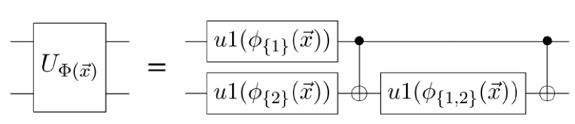
Figure 1: Quantum circuit of $U_{\Phi(\bm{x})}$ with the encoding function $\Phi(\bm{x})=\{\phi_{1}(\bm{x}),\phi_{2}(\bm{x}),\phi_{1,2}(\bm{x})\}$, composed of the three phase-shift gates of the form $u1(\phi)={\rm diag}\{1,e^{-i\phi}\}$ and two Controlled-NOT gates.

In this paper, we study the 2-qubit classifier proposed in havlivcek2019 ; an input data $\bm{x}\in\mathbb{R}^{\tilde{n}}$ is mapped to the unitary operator $\mathcal{U}_{\Phi(\bm{x})}$, which is composed of two layers of Hadamard gate $H^{\otimes 2}$ and the unitary gate $U_{\Phi(x)}$ as follows:

$$\mathcal{U}_{\Phi(\bm{x})}=U_{\Phi(\bm{x})}H^{\otimes 2}U_{\Phi(\bm{x})}H^{\otimes 2},$$ (5)

where

$$U_{\Phi(\bm{x})}=\exp\Big{(}i\phi_{1}(\bm{x})ZI+i\phi_{2}(\bm{x})IZ+i\phi_{1,2}(\bm{x})ZZ\Big{)},$$ (6)

and $\Phi(\bm{x})=\{\phi_{1}(\bm{x}),\phi_{2}(\bm{x}),\phi_{1,2}(\bm{x})\}$ is the set of encoding functions. The quantum circuit representation realizing this unitary gate is shown in Fig. 1. The three user-defined encoding functions $\phi_{1}(\bm{x}),\phi_{2}(\bm{x})$, and $\phi_{1,2}(\bm{x})$ nonlinearly transform the input data $\bm{x}$ into the qubit $\ket{\Phi(\bm{x})}=\mathcal{U}_{\Phi(\bm{x})}\ket{0}^{\otimes 2}$. A lengthy calculation then gives the explicit Pauli decomposed form (3) of the density operator $\rho(\bm{x})=\ket{\Phi(\bm{x})}\bra{\Phi(\bm{x})}$; the coefficients $\{a_{i}(\bm{x})\}$ with $i=II,XI,YI,\ldots,ZZ$ are listed in Table 1. The coefficients are composed of bunch of trigonometric functions, which make the kernel complicated enough to transform the input data highly nonlinearly.

Table 1: Coefficients of the density operator (3) in the setup shown in Section 2.2; that is, $\{a_{i}(\bm{x})\}$ with $i=II,XI,YI,\ldots,ZZ$.

Index $i$	Pauli decomposition coefficients $a_{i}$
II	$1/4$
XI	$\{\sin{\phi_{1}}(\sin{\phi_{2}}\sin{\phi_{1,2}}^{2}+\sin{\phi_{1}}\cos{\phi_{1,2}}^{2}+\cos{\phi_{2}}\cos{\phi_{1}}\sin{\phi_{1,2}})\}/4$
YI	$\{-\sin{\phi_{2}}\cos{\phi_{1}}\sin{\phi_{1,2}}^{2}-\sin{\phi_{1}}\cos{\phi_{1}}\cos{\phi_{1,2}}^{2}+\cos{\phi_{2}}\sin{\phi_{1}}^{2}\sin{\phi_{1,2}}\}/4$
ZI	$\cos{\phi_{1}}\cos{\phi_{1,2}}/4$
IX	$\{\sin{\phi_{2}}(\sin{\phi_{1}}\sin{\phi_{1,2}}^{2}+\sin{\phi_{2}}\cos{\phi_{1,2}}^{2}+\cos{\phi_{1}}\cos{\phi_{2}}\sin{\phi_{1,2}})\}/4$
XX	$\{\sin{\phi_{1}}^{2}\sin{\phi_{2}}^{2}+\sin{\phi_{1,2}}\cos{\phi_{1}}\cos{\phi_{2}}(\sin{\phi_{1}}+\sin{\phi_{2}})\}/4$
YX	$\{-\sin{\phi_{2}}^{2}\sin{\phi_{1}}\cos{\phi_{1}}+\sin{\phi_{1,2}}\cos{\phi_{2}}(\sin{\phi_{1}}\sin{\phi_{2}}-\cos{\phi_{1}}^{2})\}/4$
ZX	$\{\cos{\phi_{1,2}}(-\sin{\phi_{1}}\cos{\phi_{2}}\sin{\phi_{1,2}}+\cos{\phi_{1}}\sin{\phi_{2}}^{2}+\sin{\phi_{2}}\cos{\phi_{2}}\sin{\phi_{1,2}})\}/4$
IY	$\{-\sin{\phi_{1}}\cos{\phi_{2}}\sin{\phi_{1,2}}^{2}-\sin{\phi_{2}}\cos{\phi_{2}}\cos{\phi_{1,2}}^{2}+\cos{\phi_{1}}\sin{\phi_{2}}^{2}\sin{\phi_{1,2}}\}/4$
XY	$\{-\sin{\phi_{1}}^{2}\sin{\phi_{2}}\cos{\phi_{2}}+\sin{\phi_{1,2}}\cos{\phi_{1}}(\sin{\phi_{1}}\sin{\phi_{2}}-\cos{\phi_{2}}^{2})\}/4$
YY	$\{\sin{\phi_{1}}\cos{\phi_{1}}\sin{\phi_{2}}\cos{\phi_{2}}-\sin{\phi_{1,2}}(\cos{\phi_{2}}^{2}\sin{\phi_{1}}+\sin{\phi_{2}}\cos{\phi_{1}}^{2})\}/4$
ZY	$\{\sin{\phi_{2}}(-\sin{\phi_{1}}\sin{\phi_{1,2}}\cos{\phi_{1,2}}-\cos{\phi_{2}}\cos{\phi_{1}}\cos{\phi_{1,2}}+\sin{\phi_{2}}\cos{\phi_{1,2}}\sin{\phi_{1,2}})\}/4$
IZ	$\cos{\phi_{2}}\cos{\phi_{1,2}}/4$
XZ	$\{\cos{\phi_{1,2}}(-\sin{\phi_{2}}\cos{\phi_{1}}\sin{\phi_{1,2}}+\cos{\phi_{2}}\sin{\phi_{1}}^{2}+\sin{\phi_{1}}\cos{\phi_{1}}\sin{\phi_{1,2}})\}/4$
YZ	$\{\sin{\phi_{1}}(-\sin{\phi_{2}}\sin{\phi_{1,2}}\cos{\phi_{1,2}}-\cos{\phi_{1}}\cos{\phi_{2}}\cos{\phi_{1,2}}+\sin{\phi_{1}}\cos{\phi_{1,2}}\sin{\phi_{1,2}})\}/4$
ZZ	$\cos{\phi_{1}}\cos{\phi_{2}}/4$

2.3 Minimum accuracy

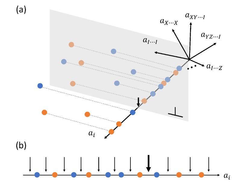
Figure 2: An example for calculating the minimum accuracy in the case of $N=10$ data points $\{\bm{a}(\bm{x}_{k})\}_{k=1,\ldots,10}$. The blue and orange points indicate the values of $y_{k}=-1$ and $y_{k}=+1$, respectively. (a) The data points are projected onto the $a_{i}$-axis in the feature space; then they are classified at a chosen threshold indicated by the arrow, which is equivalent to separating the data with the hyperplane orthogonal to the axis. (b) 1-dimensional view of the data $\{a_{i}(\bm{x}_{k})\}_{k=1,\ldots,10}$. At the same $j=8$th threshold as above, indicated by the solid arrow, we have $N_{-}=4$ and $N_{+}=3$ (the number of blue and orange points in the left side of the arrow, respectively); then the accuracy (7) is $R_{i}^{8}=0.6$. Changing the place of the threshold (i.e., the index $j$), as indicated by thin arrows, we find that the maximum of these values is $R_{i}=\max_{j}R^{j}_{i}=0.7$.

The minimum accuracy is defined as the maximum classification accuracy where the hyperplane used for classifying the training dataset is restricted to being orthogonal to any basis axis in the feature space. The main points of this definition are as follows; due to this restriction, the minimum accuracy is calculated without respect to the actual classifiers; moreover, it gives a lower bound of the accuracy for the training dataset achieved by any optimized classifier, because the optimized hyperplane is not necessarily orthogonal to any basis axis. This means that the minimum accuracy can be used to evaluate the chosen feature map and accordingly the kernel, without designing an actual classifier; in particular, if the minimum accuracy takes a relatively large value, any optimized classifier is guaranteed to achieve an equal or a higher accuracy in that feature space. Note that a similar concept is found in Ref. aronoff 1985 , which is yet defined in a different way.

In this study, the feature map is given by the vector $\bm{a}(\bm{x})=[a_{1}(\bm{x}),\ldots,a_{4^{n}}(\bm{x})]^{\top}$, and the minimum accuracy is calculated as follows, for the training dataset $\{\bm{x}_{k},y_{k}\}_{k=1,\ldots,N}$, for the case $N$ being an even number (if $N$ is an odd number, generate one more training data). In particular, we assume that the output $y_{k}=+1$ has been assigned to $N/2$ data points and $y_{k}=-1$ for the rest $N/2$ data points.

(i)

For a fixed index $i\in\{1,\cdots,4^{n}\}$, consider the dataset $\{a_{i}(\bm{x}_{k})\}_{k=1,\ldots,N}$, which are the projection of all the transformed data onto the $i$-th axis in the feature space, as shown in Fig. 2(a).

(ii)

Choose a hyperplane orthogonal to this $i$-th axis; they intersect at the threshold between a pair of neighboring projected data points, as indicated by the thick arrow in Fig.  2(a) and (b).

(iii)

Calculate the accuracy at the $j$-th threshold as follows. Let $N_{+}$ and $N_{-}$ be the number of data points with output $y_{k}=+1$ and $y_{k}=-1$ in the left side of the threshold, respectively. If $N_{+}>N_{-}$, the desirable classification pattern of the dataset is such that the points with $y_{k}=+1$ are in the left and the points with $y_{k}=-1$ are in the right; now the number of points with $y_{k}=-1$ is $N/2-N_{-}$, meaning that the classification accuracy is $(N_{+}+N/2-N_{-})/N$. (The perfect case is such that $N_{+}=N/2$ and $N_{-}=0$, leading that the accuracy is $1$.) Combining the case $N_{+}<N_{-}$, hence, the accuracy is defined by

$$R^{j}_{i}=\frac{1}{N}\Big{(}{\rm max}\{N_{+},N_{-}\}+\frac{N}{2}-{\rm min}\{N_{+},N_{-}\}\Big{)}.$$ (7)

Recall that this quantity (7) corresponds to the accuracy of classifying the dataset by the hyperplane orthogonal to the $i$-th axis at the threshold.

(iv)

Calculate the accuracy for all the thresholds with indices $j=1,\ldots,N+1$, and then take the maximum: $R_{i}=\max_{j}R^{j}_{i}$.

(v)

The minimum accuracy is defined as $R=\max_{i}R_{i}$, where the index runs from $i=1$ to $i=4^{n}$.

A simple example to demonstrate calculating the minimum accuracy is given in Fig. 2. Note that the above procedure can be readily conducted for the 2-qubit case, using the explicit form of $\{a_{i}(\bm{x})\}$ listed in Table  1.

3 Results and Discussions

3.1 Classification accuracy with different encoding functions

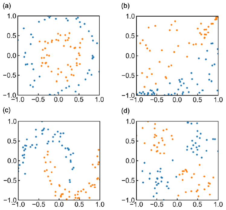
Figure 3: Dataset called (a) Circle, (b) Exp, (c) Moon, and (d) Xor.

Here we apply the quantum SVM method, with several encoding functions, to some benchmark classification problems. We consider the nonlinear 2-dimensional datasets named Circle, Exp, Moon, and Xor, shown in Fig. 3; in each case, $N=100$ data points $(\bm{x}_{k},y_{k})~{}(k=1,\ldots,100)$ are generated and categorized to two groups depending on $y_{k}=+1$ or $y_{k}=-1$ (orange or blue points in the figure). Each dataset is encoded into the 2-qubit quantum state, with the following five encoding functions:

$$\phi_{\,1}(\bm{x}) =x_{1},~{}\phi_{\,2}(\bm{x})=x_{2},~{}\phi_{\,1,2}(\bm{x})=\pi x_{1}x_{2},$$ (8)

$$\phi_{\,1}(\bm{x}) =x_{1},~{}\phi_{\,2}(\bm{x})=x_{2},~{}\phi_{\,1,2}(\bm{x})=\frac{\pi}{2}(1-x_{1})(1-x_{2}),$$ (9)

$$\phi_{\,1}(\bm{x}) =x_{1},~{}\phi_{\,2}(\bm{x})=x_{2},~{}\phi_{\,1,2}(\bm{x})=\exp\left(\frac{|x_{1}-x_{2}|^{2}}{8/\ln(\pi)}\right),$$ (10)

$$\phi_{\,1}(\bm{x}) =x_{1},~{}\phi_{\,2}(\bm{x})=x_{2},~{}\phi_{\,1,2}(\bm{x})=\frac{\pi}{3\cos(x_{1})\cos(x_{2})},$$ (11)

$$\phi_{\,1}(\bm{x}) =x_{1},~{}\phi_{\,2}(\bm{x})=x_{2},~{}\phi_{\,1,2}(\bm{x})=\pi\cos(x_{1})\cos(x_{2}).$$ (12)

The functions $\phi_{\,1,2}(\bm{x})$ are chosen from a set of various nonlinear functions in the range of $2\pi$, i.e. ${\rm max}(\phi)-{\rm min}(\phi)\leq 2\pi$ for $x_{1},x_{2}\in[-1,1]$. In particular, the coefficient of (10) and (11) are determined empirically so that the resulting classifier achieves a high accuracy on the prepared datasets. Also the reason of fixing $\phi_{\,1}(\bm{x})=x_{1}$ and $\phi_{\,2}(\bm{x})=x_{2}$ for all the encoding functions is that here we aim to investigate the dependence of the classification accuracy on $\phi_{\,1,2}(\bm{x})$. In this work, the classification accuracy are evaluated as the average accuracy of the 5-fold cross validation, where one dataset is divided into 5 groups with equal number of datasets (i.e., 20 data-points), for both the training and test dataset. All the calculations are carried out using QASM simulator included in the Qiskit package Qiskit ; to construct each element of the kernel, 10,000 shots (measurements) is performed. Also to perform the optimization procedure of SVM, scikit-learn, a popular machine learning library for Python, was employed; in particular the hyperparameter $C$ is set to $10^{10}$ for realizing the hard-margin SVM, which is the scenario where the notion of minimum accuracy is valid.

The classification accuracy of the four datasets, achieved by the above four encoding functions, are shown in Table 4(a) for the training case and Table 4(b) for the test case. Overall, the function (11) achieves good accuracy, which is larger than 0.95 for the training set and 0.88 for the test set. On the other hand, the function (8) does not always work well for classification; this function achieves the accuracy 1.00 for the training dataset of Circle and Xor, whereas the accuracy for the training Moon dataset is decreased to 0.85. Hence the different encoding functions, which lead to the different feature maps and kernels, may largely influence the resulting classification accuracy.

Table 2: Classification accuracy achieved by the quantum SVM method with the five different encoding functions.

encoding function	Circle	Exp	Moon	Xor
(8)	1.00	0.91	0.85	1.00
(9)	1.00	0.93	0.96	0.97
(10)	1.00	0.97	0.91	0.93
(11)	1.00	0.98	1.00	0.95
(12)	1.00	0.94	0.98	0.93

(a) Training accuracy

encoding function	Circle	Exp	Moon	Xor
(8)	0.97	0.83	0.85	0.99
(9)	0.96	0.89	0.87	0.96
(10)	1.00	0.92	0.86	0.91
(11)	1.00	0.88	0.92	0.89
(12)	1.00	0.92	0.87	0.88

(b) Test accuracy

3.2 Analysis of the feature map

Table 3: The minimum accuracy calculated only with the feature maps and the dataset.

encoding function	Circle	Exp	Moon	Xor
(8)	0.99	0.77	0.83	0.99
(9)	0.99	0.76	0.80	0.91
(10)	0.99	0.86	0.89	0.85
(11)	0.99	0.88	0.89	0.84
(12)	0.99	0.81	0.85	0.78

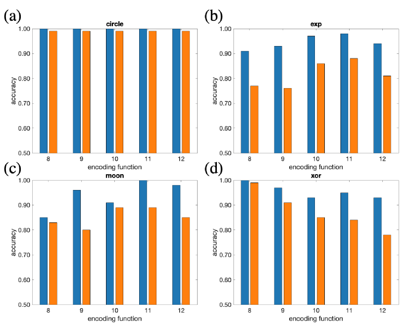
Figure 4: Comparison between the exact training accuracy in Table 4(a) (blue) and the minimum accuracy in Table 3 (orange).

Here we examine, for the classification problem described above, how the feature map $\bm{a}(\bm{x})$ would benefit us to figure out the distribution of dataset in the feature space and whether the minimum accuracy would actually predict a suitable encoding function.

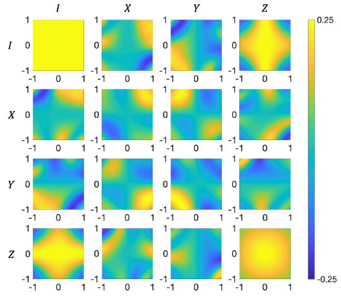
Figure 6: Color map of all the 2-dimensional spaces $a_{i}(\bm{x})$ with the encoding function (8).

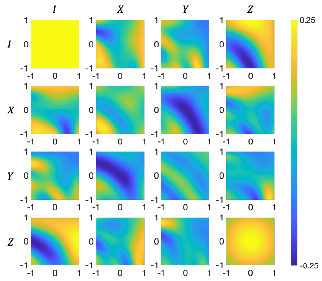
Figure 7: Color map of all the 2-dimensional spaces $a_{i}(\bm{x})$ with the encoding function (9).

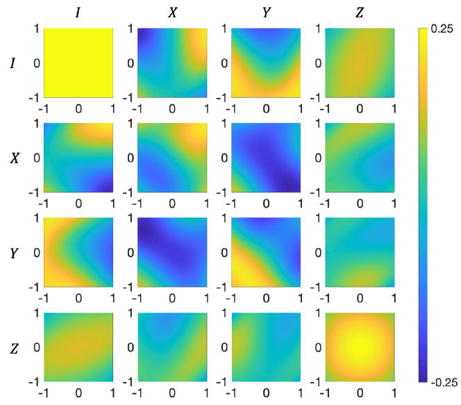
Figure 8: Color map of all the 2-dimensional spaces $a_{i}(\bm{x})$ with the encoding function (10).

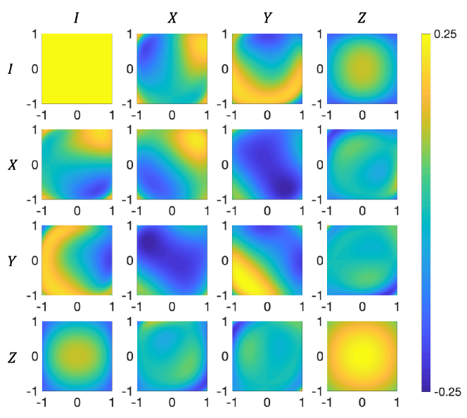
Figure 9: Color map of all the 2-dimensional spaces $a_{i}(\bm{x})$ with the encoding function (11).

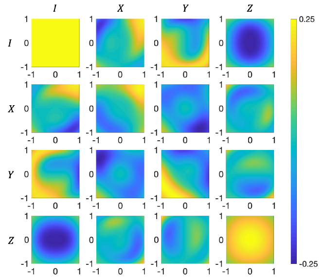
Figure 10: Color map of all the 2-dimensional spaces $a_{i}(\bm{x})$ with the encoding function (12).

First, Figs. 6-10 show the color map of $a_{i}(\bm{x})$ listed in Table 1, as a function of $\bm{x}\in\mathbb{R}^{2}$ with $i=II,XI,YI,\ldots,ZZ$ for the encoding functions (8)-(12), respectively. Note that each $a_{i}(\bm{x})$ is not determined from a specific input dataset. Nevertheless, very interestingly, some of those 2-dimensional spaces intrinsically possess the shape of distribution of the coming input dataset, which will thus affect on the resulting classification accuracy. For example, in all cases of Figs. 6-10 the ZZ element $a_{ZZ}(\bm{x})$ has a circle shape, meaning that Circle dataset can be classified only by $a_{ZZ}(\bm{x})$; this observation is consistent with the fact that Circle dataset can be indeed classified with high training/test accuracies as shown in Tables 4(a) and 4(b). Similar results can also be clearly found in Fig. 6 (the case of encoding function (8)) and in Fig. 9 (the case of (11)); the shape of $a_{YX}(\bm{x})$ in Fig. 6 has a similar distribution to Xor dataset, and actually (8) achieves the best training accuracy 1.00 for Xor dataset; the shape of $a_{YI}(\bm{x})$ in Fig. 9 has a similar distribution to Exp dataset, and actually (11) achieves the high training accuracy 0.98 for Exp dataset.

Next, Table 3 gives the minimum accuracy for the encoding functions (8)-(12), which are calculated according to the procedure given in Section 2.3. Recall that the minimum accuracy gives a lower bound of the exact training accuracy achieved by any optimized classifier, or in other words, it guarantees a worst-case accuracy. Hence, the minimum accuracy may be used as a guide to determine the feature map; that is, the encoding function with the largest minimum accuracy is recommended. Then, for Moon dataset, Table 3 suggests the encoding functions (10) or (11); similarly, for Exp and Xor datasets, (11) and (8) are recommended, respectively. Also, for the case of Circle dataset, any encoding function can be used.

Now let us compare the minimum accuracy with the exact training accuracies given in Table 4(a), to see if the above suggestions are consistent to the actual classification performance achieved by the quantum SVM. Figure 4 gives the summary, where the minimum and exact accuracies are indicated with the orange and blue bars, respectively. Importantly, the encoding function selected according to the aforementioned guide based on the minimum accuracy produce the best training accuracies; hence, as expected, the minimum accuracy may be used as a convenient measure for determining a suitable encoding function and accordingly a good feature map. Also in many cases we find positive correlation in the minimum accuracy and the exact accuracy. In particular we here consider the following simple definition; in each dataset (b), (c), and (d), a pair of functions are positively correlated if the order of their minimum accuracies is the same as that of their exact accuracies. For instance, for all the cases (b), (c), and (d), the function (11) has a higher minimum accuracy than (12), and this order holds also for the exact accuracy; hence they are positively correlated. In fact, except the pair (10) and (11) in (c), the ratio of positively correlated functions is $23/29\approx 79\%$. This fact also supports the validity of the use of minimum accuracy as a reasonable guide for choosing the encoding function.

3.3 Synthesis of the feature map via the combined Kernel method: Toward ensemble learning

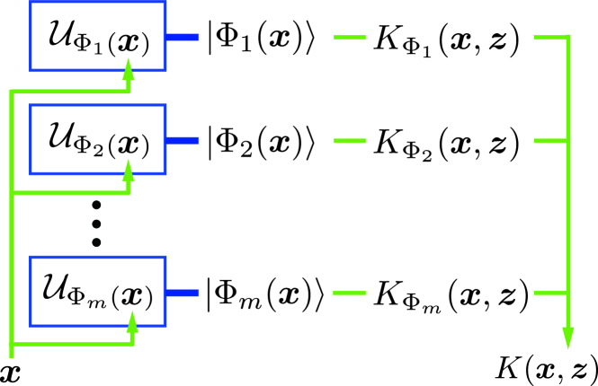
Figure 5: Scheme of the kernel synthesizer composed of different (weak) quantum computers.

Table 4: Training and Test accuracies via the classifier with combined kernels.

Encoding function	(8) + (9)	(8) + (10)	(8) + (11)	(8) + (12)
Training	1.00	0.94	1.00	1.00
Test	0.95	0.90	0.98	0.96

(a) Classification accuracies for Moon dataset

Encoding function	(8) + (9)	(8) + (10)	(8) + (11)	(8) + (12)
Training	0.96	0.93	0.95	0.95
Test	0.92	0.90	0.88	0.92

(b) Classification accuracies for Exp dataset

In the classical regime there have been a number of works on designing efficient kernels; a simple strategy is to combine some different kernels to construct a single kernel, so that the constructed one might have a desired characteristic by compensating the weakness of each kernel Bishop2006 . Here we demonstrate that this idea works in quantum regime as well, as actually in the above sections we have introduced several types of encoding functions which indeed lead to different kernel functions and accordingly different classification performances. Note that the idea of combined kernel for quantum classifier was briefly addressed in Chatterjee 2017 yet without concrete demonstration.

A typical combining method of kernels is to take a summation of them, as illustrated in Fig. 5:

$$K(\bm{x},\bm{z})=\sum_{i=1}^{m}\lambda_{i}K_{\Phi_{i}}(\bm{x},\bm{z}),$$

where $\lambda_{i}$ are the weighting parameters satisfying $\sum_{i=1}^{m}\lambda_{i}=m$ with $0\leq\lambda_{i}\leq m$ (normalization of $\{\lambda_{i}\}$ does not lead to any essential difference). Here, to demonstrate this idea, we consider the combination of two equally-weighted kernels, i.e., the case of $m=2$ and $\lambda_{1}=\lambda_{2}=1$; see Lanckriet2004 ; Dios2007 for the validity of this choice in the classical case. Even in this simple case a possible advantage may be readily seen; that is, a sum of kernels theoretically results in a higher dimensional feature space than that of the original ones as follows:

$$K_{\Phi_{1}}(\bm{x},\bm{z})+K_{\Phi_{2}}(\bm{x},\bm{z}) =|\braket{\Phi_{1}(\bm{x})}{\Phi_{1}(\bm{z})}|^{2}+|\braket{\Phi_{2}(\bm{x})}{\Phi_{2}(\bm{z})}|^{2}$$

$$=|\braket{\Phi_{1}\oplus\Phi_{2}(\bm{x})}{\Phi_{1}\oplus\Phi_{2}(\bm{z})}|^{2},$$

where $\ket{\Phi_{1}\oplus\Phi_{2}(\bm{x})}=\ket{\Phi_{1}(\bm{x})}\oplus\ket{\Phi_{2}(\bm{x})}$, meaning that the classical data $\bm{x}\in\mathbb{R}^{\tilde{n}}$ is encoded into the direct sum of two Hilbert spaces and hence the dimension of the feature space is doubled. Here we consider the same benchmark classification problems as above, by applying the 2-qubit classifier with the kernel constructed from the encoding function (8) and the other four. In this case $\bm{a}(\bm{x})$ is a 32 dimensional real vector, but with two redundant elements $a_{II}$ and $a_{ZZ}$.

We first see how much the combined kernel may improve the classification accuracy for Moon dataset for which the classifier using the single encoding function (8) showed the worst training accuracy 0.85. The resultant classification accuracies obtained by applying the combined kernels are shown in Table 6(a); every kernel results in improving the classification accuracy. Especially, when combining the weak classifiers with the kernels (8) and (10), in which case the training accuracy is 0.85 and 0.91 respectively, the classifier with this new constructed kernel achieves the accuracy 0.94. This would make sense, because the feature space visualized by $a_{i}(\bm{x})$ of the encoding functions (8) and (10) look very different, indicating that the advantages of each classifiers might be well synthesized to achieve better classification.

Similarly, we test four combined kernels composed of the encoding function (8) and the others, to classify Exp dataset for which the single encoding function (8) led to the worst training accuracy 0.91. The resultant classification accuracies are shown in Table 6(b). In this situation, however, some of the classification performance were not so improved compared to the results using the original encoding function. This issue might be resolved by carefully choosing the weighting parameters $\{\lambda_{i}\}$ when synthesizing the kernels.

A broad concept behind what we have demonstrated here is the so-called ensemble learning Dietterich2000 , which is a general and effective strategy to combine several weak classifiers to generate a single stronger classifier. Actually some quantum extension of this method have been deeply investigated in Schuld2018 ; Ximing2019 . In our work, each classifier is weak in the sense that their circuit depth and the number of qubits are severely limited; also the difference of weak classifiers simply comes from the difference of encoding functions, and the single stronger classifier is constructed merely by taking the summation of the corresponding kernels. Systematic strategy for synthesizing weak classifiers for producing a single stronger one is important particularly in the current status where only noisy intermediate-scale quantum devices are available.

4 Conclusion

In this paper, we proposed a method that helps us to analyze and synthesize the feature map for the 2-qubit kernel-based quantum classifier, based on the real-valued representation of it; the minimum accuracy, which serves as a lower bound of the exact accuracy achieved by any optimized classifier, was introduced as a tool to effectively screen a library of feature maps suitable for classification; also the method of combining (weak) feature maps to produce a better-performing map was demonstrated with some benchmarking classification problems. It is important to extend the presented method, beyond a demonstration, to a general and systematic one for constructing a quantum classifier which fully makes use of its intrinsic power.

We finally remark that, although calculating the minimum accuracy $R=\max_{i}R_{i}$ $(i=1,\ldots,4^{n})$ is intractable when $n\gg 1$, there might be some circumventing approaches. For instance, we may take $\underline{R}=\max_{i\in{\cal I}}R_{i}$ where the elements of ${\cal I}$ are randomly chosen from all $i\in\{1,\ldots,4^{n}\}$; because $\underline{R}$ also serves as a measure to evaluate the worst case accuracy for any optimized classifier, it is interesting to investigate how to construct ${\cal I}$ to have a good measure while keeping the size of ${\cal I}$ tractable. Another interesting direction is to study the connection to the quantum random access coding Ambainis ; Iwama , which discusses the method encoding large-size classical bits into small-size quantum bits; hence it is expected that even a relatively small-size quantum classifier such that $R$ can be calculated in a reasonable time might have some quantum advantages. We will work out these problems in the future.

- (1) Hastie, T., Tibshirani, R., Friedman, J.H. The elements of statistical learning: data mining, inference, and prediction, 2nd Edition. Springer series in statistics. Springer (2009)
- (2) Alpaydin, E.: Machine Learning: The New AI. MIT Press Essential Knowledge. MIT Press, Cambridge, MA (2016)
- (3) Boser, B.E., Guyon, I.M., Vapnik, V.N. : A Training Algorithm for Optimal Margin Classifiers. Proceedings of the Fifth Annual Workshop on Computational Learning Theory, 5, pp. 144-152, (1992)
- (4) Rebentrost, P., Mohseni, M., Lloyd, S.: Quantum support vector machine for big data classification. Phys. Rev. Lett. 113, 130503 (2014)
- (5) Mitarai, K., Negoro, M., Kitagawa, M., Fujii, K.: Quantum circuit learning. Phys. Rev. A 98, 032309 (2018)
- (6) Farhi, E., Neven, H.: Classification with quantum neural networks on near term processors. arXiv:1802.06002 (2018).
- (7) Zhuang, Q., Zhang, Z.: Supervised learning enhanced by an entangled sensor network. arXiv:1901.09566 (2019)
- (8) Wilson, C. M., Otterbach, J. S., Tezak, N., Smith, R. S., Crooks, G. E., da Silva, M. P.: Quantum kitchen sinks: An algorithm for machine learning on near-term quantum computers. arXiv:1806.08321 (2018)
- (9) Chatterjee, R., Yu, T.: Generalized coherent states, reproducing kernels, and quantum support vector machines. Quantum Inf. Commun. 17, 1292 (2017).
- (10) Bishwas, A.K., Mani, A., Palade, V.: An all-pair quantum SVM approach for big data multiclass classification. Quantum Information Processing 17 (10), 282 (2018)
- (11) Li, T., Chakrabarti, S., Wu, X.: Sublinear quantum algorithms for training linear and kernel-based classifiers. In: Proceedings of the 36th International Conference on Machine Learning (ICML 2019), vol. PMLR 97, pp. 3815–3824 (2019)
- (12) Havlíček, V., Córcoles, A.D., Temme, K., Harrow, A.W., Kandala, A., Chow, J.M., Gambetta, J.M.: Supervised learning with quantum-enhanced feature spaces. Nature 567 (7747), 209 (2019)
- (13) Schuld, M., Killoran, N.: Quantum machine learning in feature Hilbert spaces. Phys. Rev. Lett. 122, 040504 (2019)
- (14) Bartkiewicz, K., Gneiting, C., Černoch, A., Jiráková, K., Lemr, K., Nori, F.: Experimental kernel-based quantum machine learning in finite feature space. arXiv:1906.04137v1 (2019)
- (15) Blank, C., Park, D. K., Rhee, J. K. K., Petruccione, F.: Quantum classifier with tailored quantum kernel. arXiv:1909.02611 (2019)
- (16) T. Kusumoto, K. Mitarai, K. Fujii, M. Kitagawa, and M. Negoro, Experimental quantum kernel machine learning with nuclear spins in a solid, arXiv:1911.12021 (2019)
- (17) Lloyd, S., Schuld, M., Ijaz, A., Izaac, J., Killoran, N.: Quantum embeddings for machine learning. arXiv:2001.03622 (2020)
- (18) LaRose, R., Coyle, B.: Robust data encodings for quantum classifiers. arXiv:2003.01695 (2020)
- (19) S. Aronoff, The minimum accuracy value as an index of classification accuracy, Photogrammetric Engineering and Remote Sensing 51 (1), 99–111 (1985)
- (20) Aleksandrowicz, G., Alexander, T., Barkoutsos, P., Bello, L., Ben-Haim, Y., Bucher, D., Cabrera-Hernández, F.J., Carballo-Franquis, J., Chen, A., Chen, C.F., Chow, J.M., Córcoles-Gonzales, A.D., Cross, A.J., Cross, A., Cruz-Benito, J., Culver, C., González, S.D.L.P., Torre, E.D.L., Ding, D., Dumitrescu, E., Duran, I., Eendebak, P., Everitt, M., Sertage, I.F., Frisch, A., Fuhrer, A., Gambetta, J., Gago, B.G., Gomez-Mosquera, J., Greenberg, D., Hamamura, I., Havlicek, V., Hellmers, J., Herok, Ł., Horii, H., Hu, S., Imamichi, T., Itoko, T., Javadi-Abhari, A., Kanazawa, N., Karazeev, A., Krsulich, K., Liu, P., Luh, Y., Maeng, Y., Marques, M., Martín-Fernández, F.J., McClure, D.T., McKay, D., Meesala, S., Mezzacapo, A., Moll, N., Rodríguez, D.M., Nannicini, G., Nation, P., Ollitrault, P., O’Riordan, L.J., Paik, H., Pérez, J., Phan, A., Pistoia, M., Prutyanov, V., Reuter, M., Rice, J., Davila, A.R., Rudy, R.H.P., Ryu, M., Sathaye, N., Schnabel, C., Schoute, E., Setia, K., Shi, Y., Silva, A., Siraichi, Y., Sivarajah, S., Smolin, J.A., Soeken, M., Takahashi, H., Tavernelli, I., Taylor, C., Taylour, P., Trabing, K., Treinish, M., Turner, W., Vogt-Lee, D., Vuillot, C., Wildstrom, J.A., Wilson, J., Winston, E., Wood, C., Wood, S., Wörner, S., Akhalwaya, I.Y., Zoufal, C.: Qiskit: An open-source framework for quantum computing (2019)
- (21) Bishop, C. M.: Pattern recognition and machine learning (information science andstatistics). springer-Verlag New York, Inc., Secaucus, NJ, (2006)
- (22) Lanckriet, G. R., Cristianini, N., Bartlett, P., Ghaoui, L. E., Jordan, M. I.: Learning the kernel matrix with semidefinite programming. Journal of Machine learning research 5, pp. 27–72 (2004)
- (23) Dioş, L., Oltean, M., Rogozan, A., Pecuchet, J. P.: Improving svm performance using a linear combination of kernels. In International Conference on Adaptive and Natural Computing Algorithms, pp. 218–227. Springer, Berlin, Heidelberg. (2007)
- (24) Dietterich, T. G.: Ensemble methods in machine learning. In International workshop on multiple classifier systems, pp. 1–15. Springer, Berlin, Heidelberg. (2000)
- (25) Schuld, M., Petruccione, F.: Quantum ensembles of quantum classifiers. Scientific reports 8 (1), 2772 (2018)
- (26) Wang, X., Ma, Y., Hsieh, M. H., Yung, M.: Quantum speedup in adaptive Boosting of binary classification. arXiv:1902.00869 (2019)
- (27) A. Ambainis, A. Nayak, A. Ta-shma, and U. Vazirani, Dense quantum coding and a lower bound for 1-way quantum automata, J. ACM, 49, 496–511 (2002)
- (28) K. Iwama, H. Nishimura, R. Raymond, S. Yamashita, Unbounded-error one-way classical and quantum communication complexity, Automata, Languages and Programming, Lecture Notes in Computer Science, 4596. Springer, Berlin, Heidelberg (2007)