General solutions of the leakage in integral transforms and applications to the EB-leakage and detection of the cosmological gravitational wave background

Abstract

For an orthogonal integral transform with complete dataset, any two components are linearly independent; however, when some data points are missing, there is going to be leakage from one component to another, which is referred to as the “leakage in integral transforms” in this work. A special case of this kind of leakage is the EB-leakage in detection of the cosmological gravitational wave background (CGWB). I first give the general solutions for all integral transforms, prove that they are the best solutions, and then apply them to the case of EB-leakage and detection of the CGWB. In the upcoming decade, most likely, new cosmic microwave background (CMB) data are from ground/balloon experiments, so they provide only partial sky coverage. Even in a fullsky mission, due to the Galactic foreground, part of the sky is still unusable. Within this context, the EB-leakage becomes inevitable. I show how to use the general solutions to achieve the minimal error bars of the EB-leakage, and use it to find out the maximum ability to detect the CGWB through CMB. The results show that, when focusing on the tensor-to-scalar ratio $r$ (at a pivot scale of 0.05 Mpc^-1), $1\%$ sky coverage ($f_{sky}=1\%$) is enough for a $5\sigma$-detection of $r\geq 10^{-2}$, but is barely enough for $r=10^{-3}$. If the target is to detect $r\sim 10^{-4}$ or $10^{-5}$, then $f_{sky}\geq 10\%$ is strongly recommended to enable a $5\sigma$-detection and to reserve some room for other errors.

1 Introduction

The B-mode polarization of the CMB provides the most probable way of detecting the CGWB, but the ability of detection is limited by the quality of foreground removal, noise reduction, systematics control, delensing and EB-leakage correction. In the coming decade, a practical constraint for detecting the CGWB is that: Because all running experiments are ground based, for several years there is going to be no new fullsky CMB data. Even when one tries to combine the data of several ground experiments, there are still problems like channel differences, systematics differences, observational time allocation, etc. Therefore, in the near future, the detection of the CGWB through CMB has to be done with a limited sky coverage.

When the sky is incomplete, there is going to be leakage from the much stronger E-mode signal to the desired B-mode signal [1, 2], called the EB-leakage. This leakage will seriously contaminate the primordial B-mode signal, so it must be corrected before detecting the CGWB. It is reasonable to expect that, given an incomplete sky coverage, there is going to be an unbeatable minimal error coming from the EB-leakage, which will set an upper limit of the ability to detect the CGWB, even if all other issues are perfectly solved. In [3, 4], we presented the best blind estimate (BBE) of the EB-leakage, but one problem still remains: when there is some reasonable prior information, can we improve the estimation of the EB-leakage? If the answer is yes, to what extent?

To answer this question, we should first give a very brief review of the commonly used method of estimation in CMB science. Given a sky map $\bm{P}=\{x_{1},x_{2},\cdots,x_{n}\}$ that can be described by a set of model parameters $\bm{\Theta}=\{\theta_{1},\theta_{2},\cdots\,\theta_{m}\}$, a typical parameter estimation problem is called a posterior estimation, which tries to find $\bm{\Theta}$ that can maximize the conditional probability $P(\bm{\Theta}|\bm{P})$ with given $\bm{P}$. It was clearly described in [5], given a sky map $\bm{P}$, how to design the posterior best unbiased estimate (BUE) by using the Fisher information matrix. Later in [6], the estimation of $\bm{\Theta}$ was given in a different way using the maximum likelihood approach. In appendix B, I provide a step-by-step proof that, for a Gaussian isotropic CMB signal, the Fisher estimator and the maximum likelihood estimator give identical results. Thus the problem of posterior estimation in CMB is clear and sufficiently studied.

However, one thing has to be noticed: if some data points are missing, then even a “posterior estimation” can not be 100% posterior. There must be some additional constraints/information about the missing data, otherwise the error of estimates does not converge. For example, Gaussianity and isotropy of the CMB signal are explicitly assumed in [5]. Below I argue that, in addition to Gaussianity and isotropy, for the problem of EB-leakage, the EE-spectrum can serve as perfect prior information:

1. Currently in CMB experiments, the EE-spectrum is known much better than the mysterious BB-spectrum. Especially, the Planck mission already gave an excellent EE-spectrum by full sky surveys [7, 8].

2. Even if the EE-spectrum is slightly imperfect, there is no problem to assume an ideal EE-spectrum to give an ideal lower limit of the EB-leakage error bars, which is still very useful.

3. Practically, the estimation with prior information is not sensitive to small variations of the EE-spectrum. Thus small imperfections are not really important.

Therefore, with the best EE-spectrum given by Planck as the prior information, it is expected that the BBE of the EB-leakage can be improved. In fact, the solutions to this problem work not only for the EB-leakage, but also for all kinds of integral transforms, thus this work is arranged as the following: I start from the general case for all integral transforms, derive the general solutions for both BBE and BUE, and give detailed proofs (sections 2–3). Then the solution is applied to the case of EB-leakage to give an estimation of the maximum ability of detecting the CGWB through CMB (section 4). Finally, a brief discussion is given in section 5.

2 Context and notations

To give a clear definition of “leakage due to missing data in integral transforms”, we should start from introducing the mathematical environment.

Let $\bm{\Omega}$ be an $n$-dimensional space, $\bm{p}=(x_{1},x_{2},\cdots,x_{n})$ be one point in $\bm{\Omega}$, $\bm{\omega}$ be a subset of $\bm{\Omega}$ containing points $\{\bm{p}_{1},\bm{p}_{2},\cdots\}$, and $g=\{g_{1}(\bm{p}),g_{2}(\bm{p}),\cdots\}_{\bm{p}\in\bm{\omega}}$ be a set of complete and normalized basis functions defined on $\bm{\omega}$. Based on $g$, the integral transform of a function $f(\bm{p})_{\bm{p}\in\bm{\omega}}$ (shortened as $f(\bm{p})$ hereafter) is

$$a_{i}=\int_{\bm{\omega}}f(\bm{p})g_{i}^{*}(\bm{p})\,d\bm{p}.$$ (2.1)

Depending on the type of the integral transform, some conditions might be required to ensure the convergence of the integral transform, e.g., the Dirichlet conditions for Fourier transform. Normally, in the discrete case, most such conditions can be ignored or at least weakened, which is very convenient.

If the integral transforms are orthogonal, then we have

$$\int_{\bm{\omega}}g_{i}(\bm{p})g_{j}^{*}(\bm{p})\,d\bm{p} = \left\{\begin{array}[]{lr}1&(i=j)\\ 0&(i\neq j)\end{array}\right..$$ (2.4)

This is also convenient, because it means $f(\bm{p})$ can be uniquely decomposed into the summation of several components:

$$f(\bm{p})=\sum_{i}a_{i}g_{i}(\bm{p})=\sum_{i}G_{i}(\bm{p}),$$ (2.5)

where $G_{i}(\bm{p})=a_{i}g_{i}(\bm{p})$ is the $i$-th component of $f(\bm{p})$. Note that here the decomposition is written in a discrete form, whereas for the continuous form, the summation becomes integration.

For convenience, the operation of extracting $G_{i}(\bm{p})$ from a function $f(\bm{p})$ is shortened as

$$\Psi_{i}(\bm{f})\Rightarrow G_{i}(\bm{p}).$$ (2.6)

When the data on some points are missing, the rest of the available points forms a subset of $\bm{\omega}$ called $\bm{\omega}_{1}$. For convenience, this is represented by a mask $\bm{M}(\bm{p})$ defined as

$$\bm{M}(\bm{p}) = \left\{\begin{array}[]{lr}1&(\bm{p}\in\bm{\omega}_{1})\\ 0&(\bm{p}\notin\bm{\omega}_{1})\end{array}\right..$$ (2.9)

When the mask $\bm{M}(\bm{p})$ is present, the $i$-th component and the $j$-th component of the integral transform are normally non-orthogonal. Thus the $j$-th component derived with a mask will also receive a contribution from the $i$-th component. This is called the $i$-to-$j$ leakage $\bm{L}_{ji}(\bm{p}_{1},\bm{p}_{2},\cdots,\bm{q}_{1},\bm{q}_{2},\cdots)$, where $\bm{p}_{i}\in\bm{\omega}_{1}$ and $\bm{q}_{i}\notin\bm{\omega}_{1}$ are the available and unavailable points, respectively. For example, when $i$ represents the CMB E-mode and $j$ represents the CMB B-mode, $\bm{L}_{ji}$ is called the EB-leakage.

A precise estimation of $\bm{L}_{ji}$ cannot be achieved as it requires both $\bm{p}_{i}$ and $\bm{q}_{i}$, however, if $\bm{L}_{ji}$ can be mathematically decomposed into

$$\bm{L}_{ji}(\bm{p}_{1},\bm{p}_{2},\cdots,\bm{q}_{1},\bm{q}_{2},\cdots)=\bm{\mathcal{L}}_{ji}(\bm{p}_{1},\bm{p}_{2},\cdots)+\bm{\Delta}_{ji}(\bm{q}_{1},\bm{q}_{2},\cdots)+\mathrm{const},$$ (2.10)

where $\bm{\mathcal{L}}_{ji}$ and $\bm{\Delta}_{ji}$ depend only on the available and unavailable points, respectively, then $\bm{\mathcal{L}}_{ji}$ is the best blind estimate, because any improvement of $\bm{\mathcal{L}}_{ji}$ requires additional information of the unavailable points, which is impossible in the blind case. With the Taylor series expansion of $\bm{L}_{ji}$, one can easily prove that, if eq. (2.10) exists, then $\bm{\mathcal{L}}_{ji}$ is unique. Therefore, if the BBE exists, then it is also unique (allowing a trivial constant offset).

In a real experiment, it is possible that, although some points are missing, one still knows some prior information about them, e.g., they are expected to be Gaussian and isotropic. An estimation can be done either without or with prior information $\bm{\mathcal{I}}$ of the missing points, called the blind and non-blind estimations, respectively. For the non-blind estimation, let the set of all $f(\bm{p})$ that satisfy the prior information $\bm{\mathcal{I}}$ be $\{f_{i}(\bm{p})\}_{\bm{\mathcal{I}}}$, then for convenience, I define the following covariance matrices:

$$\bm{C}_{0}(\bm{p},\bm{p}^{\prime}) = \langle f(\bm{p})f(\bm{p}^{\prime})\rangle_{\bm{\mathcal{I}}}$$ (2.11)

$$\bm{C}_{1}(\bm{p},\bm{p}^{\prime}) = \langle\bm{L}_{ji}(\bm{p})\bm{\mathcal{L}}_{ji}(\bm{p}^{\prime})\rangle_{\bm{\mathcal{I}}}$$

$$\bm{C}_{2}(\bm{p},\bm{p}^{\prime}) = \langle\bm{\mathcal{L}}_{ji}(\bm{p})\bm{\mathcal{L}}_{ji}(\bm{p}^{\prime})\rangle_{\bm{\mathcal{I}}}.$$

In the blind case, an important fact is that all the above covariance matrices do not converge. However, with the prior information $\bm{\mathcal{I}}$, it is possible for $\bm{C}_{0}(\bm{p},\bm{p}^{\prime})$ to converge. In this work, $\bm{\mathcal{I}}$ is called regular if $\bm{C}_{0}(\bm{p},\bm{p}^{\prime})$ does converge and carry all information of $\bm{\mathcal{I}}$.

3 The main results and proofs

With the above context and notation, the main results of this work are summarized below, followed by detailed proofs:

1. In the blind case, the BBE of $\bm{L}_{ji}(\bm{p})$ is unique, and is given by $\bm{\mathcal{L}}_{ji}(\bm{p})=\Psi_{j}(\bm{M}\bm{W}\Psi_{i}(\bm{M}\bm{f}))$, where $\bm{f}$ is the dataset, $\bm{M}$ is the mask, and $\bm{W}$ is an optional window function.

2. In the non-blind case, if the prior information $\bm{\mathcal{I}}$ is regular, then the BUE of $\bm{L}_{ji}(\bm{p})$ is $\bm{\mathcal{L}}^{\bm{\mathcal{I}}}_{ji}(\bm{p})=\bm{C}_{1}\cdot\bm{C}_{2}^{-1}\cdot\bm{\mathcal{L}}_{ji}(\bm{p})$.

3.1 Proof of the blind case

First substitute eq. (2.1) into eq. (2.5) to get the $i$-th component of the integral transform:

$$G_{i}(\bm{p}) = \int_{\bm{\omega}}f(\bm{p}^{\prime})g_{i}^{*}(\bm{p}^{\prime})g_{i}(\bm{p})\,d\bm{p}^{\prime}$$

$$= \int_{\bm{\omega}}\mathcal{G}_{i}(\bm{p},\bm{p}^{\prime})f(\bm{p}^{\prime})\,d\bm{p}^{\prime},$$

where $\mathcal{G}_{i}(\bm{p},\bm{p}^{\prime})=g_{i}(\bm{p})g_{i}^{*}(\bm{p}^{\prime})$ is the real-space convolution kernel for getting the $i$-th component of the integral transform. Use eq. (3.1) again to get the $j$-th component from $G_{i}(\bm{p})$, which is the $i$-to-$j$ leakage $\bm{L}^{0}_{ji}(\bm{p})$ while no data is missing:

$$\bm{L}^{0}_{ji}(\bm{p}) = \int_{\bm{\omega}}\mathcal{G}_{j}(\bm{p},\bm{p}^{\prime})G_{i}(\bm{p}^{\prime})\,d\bm{p}^{\prime}$$

$$= \int_{\bm{\omega}}\mathcal{G}_{j}(\bm{p},\bm{p}^{\prime})\left[\int_{\bm{\omega}}\mathcal{G}_{i}(\bm{p}^{\prime},\bm{p}^{\prime\prime})f(\bm{p}^{\prime\prime})\,d\bm{p}^{\prime\prime}\right]\,d\bm{p}^{\prime}$$

$$= \int_{\bm{\omega}}f(\bm{p}^{\prime\prime})\mathcal{G}_{ji}(\bm{p},\bm{p}^{\prime\prime})\,d\bm{p}^{\prime\prime},$$

where $\mathcal{G}_{ji}(\bm{p},\bm{p}^{\prime\prime})=\int_{\bm{\omega}}\mathcal{G}_{j}(\bm{p},\bm{p}^{\prime})\mathcal{G}_{i}(\bm{p}^{\prime},\bm{p}^{\prime\prime})\,d\bm{p}^{\prime}$ is the convolution kernel of the $i$-to-$j$ leakage. If the integral transform is orthogonal, and the integral is done for the entire $\bm{\omega}$ (no data is missing) and $j\neq i$, then $\mathcal{G}_{ji}(\bm{p},\bm{p}^{\prime\prime})=0$ and $\bm{L}^{0}_{ji}(\bm{p})=0$, i.e., there is no leakage.

When the data on some points are missing as described by eq. (2.9), the $i$-to-$j$ leakage $\bm{L}_{ji}(\bm{p})$ is given by getting the $j$-th component from the real $G_{i}(\bm{p}^{\prime})$ with a mask. Using the notation in eq. (2.6), this is written as

$$\bm{L}_{ji}(\bm{p})=\Psi_{j}(\bm{M}\Psi_{i}(\bm{f})),$$ (3.3)

whose integral form is

$$\bm{L}_{ji}(\bm{p}) = \int_{\bm{\omega}}\mathcal{G}_{j}(\bm{p},\bm{p^{\prime}})\left[\bm{M}(\bm{p}^{\prime})G_{i}(\bm{p}^{\prime})\right]\,d\bm{p}^{\prime}$$

$$= \int_{\bm{\omega}}\mathcal{G}_{j}(\bm{p},\bm{p^{\prime}})\bm{M}(\bm{p}^{\prime})\left[\int_{\bm{\omega}}\mathcal{G}_{i}(\bm{p}^{\prime},\bm{p}^{\prime\prime})f(\bm{p}^{\prime\prime})\,d\bm{p}^{\prime\prime}\right]\,d\bm{p}^{\prime}$$

$$= \int_{\bm{\omega}}f(\bm{p}^{\prime\prime})\mathcal{G}_{ji}(\bm{p},\bm{p}^{\prime\prime})_{\bm{\omega_{1}}}\,d\bm{p}^{\prime\prime},$$

where

$$\mathcal{G}_{ji}(\bm{p},\bm{p}^{\prime\prime})_{\bm{\omega_{1}}} = \int_{\bm{\omega}}\mathcal{G}_{j}(\bm{p},\bm{p^{\prime}})\mathcal{G}_{i}(\bm{p}^{\prime},\bm{p}^{\prime\prime})\bm{M}(\bm{p}^{\prime})\,d\bm{p}^{\prime}$$ (3.5)

is a fixed convolution kernel, which is normally non-zero, so the leakage $\bm{L}_{ji}(\bm{p})$ is normally non-zero.

Eq. (3.1) shows that the true leakage term is the convolution of the kernel $\mathcal{G}_{ji}(\bm{p},\bm{p}^{\prime\prime})_{\bm{\omega_{1}}}$ with $f(\bm{p}^{\prime\prime})$ on the entire $\bm{\omega}$, which cannot be done for the missing part of the data. In reality, this integral can only be done for $\bm{\omega}_{1}$, which gives

$$\bm{\mathcal{L}}_{ji}(\bm{p})=\int_{\bm{\omega}}f(\bm{p}^{\prime\prime})\bm{M}(\bm{p}^{\prime\prime})\mathcal{G}_{ji}(\bm{p},\bm{p}^{\prime\prime})_{\bm{\omega}_{1}}\,d\bm{p}^{\prime\prime},$$ (3.6)

and the error $\bm{\Delta}_{ji}(\bm{p})$ is

$$\bm{\Delta}_{ji}(\bm{p})=\bm{L}_{ji}(\bm{p})-\bm{\mathcal{L}}_{ji}(\bm{p})=\int_{\bm{\omega}}f(\bm{p}^{\prime\prime})[1-\bm{M}(\bm{p}^{\prime\prime})]\mathcal{G}_{ji}(\bm{p},\bm{p}^{\prime\prime})_{\bm{\omega}_{1}}\,d\bm{p}^{\prime\prime}.$$ (3.7)

$\bm{\mathcal{L}}_{ji}(\bm{p})$ and $\bm{\Delta}_{ji}(\bm{p})$ fully satisfy eq. (2.10), thus $\bm{\mathcal{L}}_{ji}(\bm{p})$ is the unique BBE.

Calculation of eq. (3.6) is difficult, because it is normally computationally intensive to obtain $\mathcal{G}_{ji}(\bm{p},\bm{p}^{\prime\prime})_{\bm{\omega}_{1}}$. A much faster way of doing the same thing is to calculate $\bm{\mathcal{L}}_{ji}^{fast}(\bm{p})$ instead, which requires only to change the order of integration as follows:

$$\bm{\mathcal{L}}_{ji}(\bm{p}) = \int_{\bm{\omega}}f(\bm{p}^{\prime\prime})\bm{M(\bm{p}^{\prime\prime})}\mathcal{G}_{ji}(\bm{p},\bm{p}^{\prime\prime})_{\bm{\omega}_{1}}\,d\bm{p}^{\prime\prime}$$

$$= \int_{\bm{\omega}}f(\bm{p}^{\prime\prime})\bm{M(\bm{p}^{\prime\prime})}\left[\int_{\bm{\omega}}\mathcal{G}_{j}(\bm{p},\bm{p^{\prime}})\mathcal{G}_{i}(\bm{p}^{\prime},\bm{p}^{\prime\prime})\bm{M}(\bm{p}^{\prime})\,d\bm{p}^{\prime}\right]\,d\bm{p}^{\prime\prime}$$

$$= \int_{\bm{\omega}}\mathcal{G}_{j}(\bm{p},\bm{p}^{\prime})\bm{M(\bm{p}^{\prime})}\left[\int_{\bm{\omega}}\mathcal{G}_{i}(\bm{p}^{\prime},\bm{p}^{\prime\prime})f(\bm{p}^{\prime\prime})\bm{M(\bm{p}^{\prime\prime})}\,d\bm{p}^{\prime\prime}\right]\,d\bm{p}^{\prime}$$

$$= \bm{\mathcal{L}}_{ji}^{fast}(\bm{p}).$$

Based on the above equation and using the notation in eq. (2.6), the analytic form of the unique BBE that is easy to calculate is:

$$\bm{\mathcal{L}}_{ji}(\bm{p})\equiv\bm{\mathcal{L}}_{ji}^{fast}(\bm{p})=\Psi_{j}(\bm{M}\Psi_{i}(\bm{M}\bm{f})).$$ (3.9)

Eq. (3.9) is easy to calculate because it can be done by standard forward-backward integral transforms. Therefore, the BBE can be easily obtained as long as a fast algorithm of the integral transform is available, e.g., the fast Fourier transforms (FFT). This is extremely convenient, and is exactly the idea of the recycling method used in [3] to correct the EB-leakage for detecting the CGWB.

It is also possible to use an extra window function $\bm{W}(\bm{p})$ that smooths the edge of the region, which is the conventional way of reducing the leakage. It is important to note that the window function is defined only in the available region, and it can never change the unavailable region to available. Therefore, using the window function is equivalent to replacing $\bm{M}(\bm{p}^{\prime})$ by $\bm{M}(\bm{p}^{\prime})\bm{W}(\bm{p}^{\prime})$ in eq. (3.1) and eq. (3.1) (without touching $\bm{M}(\bm{p}^{\prime\prime})$). Consequently, eq. (3.9) becomes

$$\bm{\mathcal{L}}_{ji}(\bm{p})\equiv\bm{\mathcal{L}}_{ji}^{fast}(\bm{p})=\Psi_{j}(\bm{MW}\Psi_{i}(\bm{M}\bm{f})).$$ (3.10)

3.2 Proof of the non-blind case

Now we can start to prove the conclusion for the non-blind case. For convenience, the true leakage $\bm{L}_{ji}(\bm{p})$ is shortened as a column vector $\bm{L}$. Similarly, $\bm{\mathcal{L}}_{ji}(\bm{p})$ is shortened as column vector $\bm{\mathcal{L}}$ of the same size. Hence the general form of $\bm{L}$ as a function of $\bm{\mathcal{L}}$ is

$$\bm{L}=\widetilde{\bm{L}}(\bm{\mathcal{L}})+\bm{\Lambda}(\bm{\mathcal{L}})+\bm{\Delta},$$ (3.11)

where $\widetilde{\bm{L}}(\bm{\mathcal{L}})$ is the linear part whose second and higher derivatives are zero, and $\bm{\Lambda}(\bm{\mathcal{L}})$ is the non-linear part whose first derivative is zero. $\bm{\Delta}$ is the error, which is not a function of $\bm{\mathcal{L}}$ and is statistically uncorrelated with $\widetilde{\bm{L}}(\bm{\mathcal{L}})$ and $\bm{\Lambda}(\bm{\mathcal{L}})$. The matrix form of the above equation is

$$\bm{L}=\bm{m}\cdot\bm{\mathcal{L}}+\bm{\Lambda}(\bm{\mathcal{L}})+\bm{\Delta},$$ (3.12)

where $\bm{m}$ is a constant coupling matrix.

If the prior information $\bm{\mathcal{I}}$ is regular, then $\bm{C}_{0}$ is converged and constant. Using eq. (3.1–3.6), we get

$$\bm{C}_{1} = \left\langle\int_{\bm{\omega}}f(\bm{p}^{\prime})\mathcal{G}_{ji}(\bm{p},\bm{p}^{\prime})_{\bm{\omega_{1}}}f(\bm{p}^{\prime\prime\prime})\mathcal{G}_{ji}(\bm{p}^{\prime\prime},\bm{p}^{\prime\prime\prime})_{\bm{\omega_{1}}}\bm{M}(\bm{p}^{\prime\prime\prime})\,d\bm{p}^{\prime}d\bm{p}^{\prime\prime\prime}\right\rangle_{\bm{\mathcal{I}}}$$

$$= \int_{\bm{\omega}}\mathcal{G}_{ji}(\bm{p},\bm{p}^{\prime})_{\bm{\omega_{1}}}\mathcal{G}_{ji}(\bm{p}^{\prime\prime},\bm{p}^{\prime\prime\prime})_{\bm{\omega_{1}}}\bm{M}(\bm{p}^{\prime\prime\prime})\left\langle f(\bm{p}^{\prime})f(\bm{p}^{\prime\prime\prime})\right\rangle_{\bm{\mathcal{I}}}\,d\bm{p}^{\prime}d\bm{p}^{\prime\prime\prime}$$

$$= \int_{\bm{\omega}}\mathcal{G}_{ji}(\bm{p},\bm{p}^{\prime})_{\bm{\omega_{1}}}\mathcal{G}_{ji}(\bm{p}^{\prime\prime},\bm{p}^{\prime\prime\prime})_{\bm{\omega_{1}}}\bm{M}(\bm{p}^{\prime\prime\prime})\bm{C}_{0}(\bm{p}^{\prime},\bm{p}^{\prime\prime\prime})\,d\bm{p}^{\prime}d\bm{p}^{\prime\prime\prime}$$

$$= \mathrm{const}\,.$$

Similarly, $\bm{C}_{2}$ is also constant. Using eq. (3.12) to recalculate the covariance matrix gives

$$\bm{C}_{1} = \langle\bm{L}\bm{\mathcal{L}^{T}}\rangle_{\bm{\mathcal{I}}}$$

$$= \bm{m}\cdot\langle\bm{\mathcal{L}}\bm{\mathcal{L}}^{T}\rangle_{\bm{\mathcal{I}}}+\langle\bm{\Lambda}(\bm{\mathcal{L}})\bm{\mathcal{L}}^{T}\rangle_{\bm{\mathcal{I}}}+\langle\bm{\Delta}\bm{\mathcal{L}}^{T}\rangle_{\bm{\mathcal{I}}}$$

$$= \bm{m}\cdot\bm{C}_{2},$$

thus $\bm{m}=\bm{C}_{1}\cdot\bm{C}_{2}^{-1}$ is a constant matrix, and

$$\widetilde{\bm{L}}=\bm{m}\cdot\bm{\mathcal{L}}=\bm{C}_{1}\cdot\bm{C}_{2}^{-1}\cdot\bm{\mathcal{L}}.$$ (3.15)

With the well known theory of least-square fitting, one can easily prove that eq. (3.15) is exactly the unbiased estimate with minimal variance (see Appendix A for more details). Therefore, the BUE with regular prior information $\bm{\mathcal{I}}$ is

$$\bm{\mathcal{L}}^{\bm{\mathcal{I}}}_{ji}(\bm{p})=\bm{C}_{1}\cdot\bm{C}_{2}^{-1}\cdot\bm{\mathcal{L}}_{ji}(\bm{p}).$$ (3.16)

3.3 Property of the error

In this section, the properties of the error of estimation are discussed, which gives important information about when we should apply the leakage estimation.

Starting from eq. (3.1), with mask $\bm{M}(\bm{p}^{\prime})$, we get the corrupted $i$-th component $\widetilde{G}_{i}(\bm{p})$ as

$$\widetilde{G}_{i}(\bm{p}) = \int_{\bm{\omega}}\mathcal{G}_{i}(\bm{p},\bm{p}^{\prime})f(\bm{p}^{\prime})\bm{M}(\bm{p}^{\prime})\,d\bm{p}^{\prime}$$

$$= \int_{\bm{\omega}}\mathcal{G}_{i}(\bm{p},\bm{p}^{\prime})\bm{M}(\bm{p}^{\prime})\left[\sum_{j}{G_{j}(\bm{p}^{\prime})}\right]\,d\bm{p}^{\prime}$$

$$= \int_{\bm{\omega}}\mathcal{G}_{i}(\bm{p},\bm{p}^{\prime})\bm{M}(\bm{p}^{\prime})\left[G_{i}(\bm{p}^{\prime})+\sum_{j\neq i}{G_{j}(\bm{p}^{\prime})}\right]\,d\bm{p}^{\prime}$$

$$= \int_{\bm{\omega}}\mathcal{G}_{ii}(\bm{p},\bm{p}^{\prime})_{\bm{\omega_{1}}}f(\bm{p}^{\prime})\,d\bm{p}^{\prime}+\int_{\bm{\omega}}\mathcal{G}_{i\bar{i}}(\bm{p},\bm{p}^{\prime})_{\bm{\omega_{1}}}f(\bm{p}^{\prime})\,d\bm{p}^{\prime}$$

$$= \bm{L}_{ii}(\bm{p})+\bm{L}_{i\bar{i}}(\bm{p}),$$

where $\bar{i}$ means the combination of all the $j\neq i$ components, so $\bm{L}_{ii}(\bm{p})$ is the $i$-to-$i$ leakage, and $\bm{L}_{i\bar{i}}(\bm{p})$ is the combined cross leakage from all non-$i$ components. In analogy to a square matrix, they are similar to the diagonal and off-diagonal terms.

For a set of given input data and given mask, $\widetilde{G}_{i}(\bm{p})$ is known and fixed, thus the errors of estimating $\bm{L}_{ii}(\bm{p})$ and $\bm{L}_{i\bar{i}}(\bm{p})$ satisfy

$$\Delta\bm{L}_{ii}(\bm{p})+\Delta\bm{L}_{i\bar{i}}(\bm{p})=0,$$ (3.18)

which means one can only try to optimize one estimator, and then the error of the other term is automatically fixed. In practice, if the prior information $\mathcal{I}$ shows that the $i$-th component is very weak, then apparently $\Delta\bm{L}_{i\bar{i}}(\bm{p})$ will be dominating. In this case, the overall best estimation is given by eq. (3.16).

For example, a standard integral transform of the polarized signal on the sphere includes two modes: the E-mode and the B-mode. Each of them has the same number of members. If the polarized signal is the CMB, then the prior expectation shows that all B-mode components are much weaker than the E-mode components, thus eq. (3.16) is the best choice of correcting the E-to-B leakage.

4 Application: the maximum ability to detect the CGWB through the Cosmic Microwave Background with incomplete sky coverage

As mentioned in the introduction, in the coming decade, all available CMB experiments are ground-based, which can hardly provide full sky coverage. In this case, detection of the primordial B-mode will contain an unbeatable minimal error due to the EB-leakage, even if everything else is done perfectly. This sets an absolute constraint on the ability to detect the CGWB through CMB for each choice of the sky coverage. Apparently, to find this constraint, we should use the BUE with prior information $\mathcal{I}$ in eq. (3.16), with $\mathcal{I}$ being the best available EE-spectrum.

4.1 Comparison of the BBE and the BUE

Now we proceed to testing and comparing the BBE and the BUE given in section 3 with practical calculations. We start from the best fit Planck 2018 CMB spectra to generate simulated CMB maps. Because the BUE is extremely time consuming, the simulated CMB maps are generated only at $N_{side}=64$ with $r=0.05$, and a disk mask of $f_{sky}=0.01$ is used in this test. For each simulated map, the BBE and the BUE are used to estimate the resulting B-maps, respectively, and compared the results with the real B-map (derived from the known fullsky map) within the available region. We first compare their similarities by the Pearson Cross Correlation (CC) coefficients, as shown in the left panel of Figure 1. Evidently, the result of the BUE (red line) has higher CC coefficients (better similarity) with the real B-map than the BBE does. In the right panel, I compare the BB-spectrum error of the BUE and the BBE. Note that in the test here, the focus is on the error of the EB-leakage estimation, thus the BB-spectra are calculated from the masked real B-map and the BUE/BBE B-maps directly, without reconstruction of the fullsky spectra (this will be considered later). The uncertainties of the BUE/BBE methods are computed as the rms differences between the real B-map spectrum and the BUE/BBE B-map spectra. The result shows that, when running at the same resolution, the BUE helps to reduce the error around $\ell\approx 100$ by roughly 30%.

Practically, as pointed out by [2], oversampling can help to reduce the leakage due to pixelization, and a similar effect was seen even for the temperature case, as shown in figures 4 and 6 of  [10]. Because it is much easier to increase the resolution for the BBE than for the BUE, practically, running the BBE at a much higher resolution can effectively give a comparable result to running the BUE at a relatively lower resolution. Thus running the BBE at increased resolution is likely the most practical and promising way of correcting the EB-leakage at a high resolution.

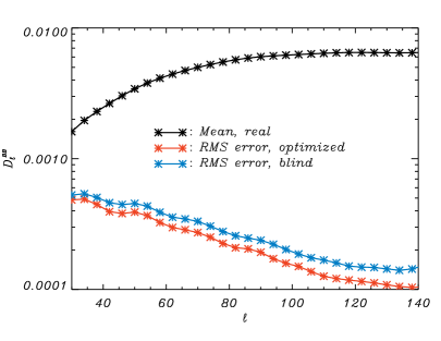
Figure 1: Left: Comparison of the similarity between the real and fixed B-maps using the Pearson Cross Correlation coefficients (CC). Red for the BUE, and blue for the BBE, represented by the recycling method in [3]. Apparently the BUE gives better similarity to the real B-map. Right: Comparison of the BB-spectrum error of the BUE and the recycling method, where $D_{\ell}=\ell(\ell+1)C_{\ell}/(2\pi)$. The BUE gives roughly 30% lower error bars around $\ell=100$.

4.2 Estimation of the maximum ability

As discussed in section 1, the maximum ability to detect the CGWB through the Cosmic Microwave Background with incomplete sky coverage can be found out by the BUE of the EB-leakage with proper prior information. The details of the idea are as follows: when only part of the sky is available, the minimal error of EB-leakage is given by the BUE in eq. (3.16), and the minimal error of recovering the full sky BB-spectrum is given by the Fisher estimator [5, 9, 11, 12, 13, 10]. Combining these two minimal errors gives the maximum ability of detecting CGWB through CMB when all other things are assumed to be perfect, except only the sky coverage is incomplete.

In practice, both the BUE in eq. (3.16) and the Fisher estimator are extremely time consuming. For a real estimation of the EB-leakage and the B-mode spectrum, one has to deal with the BUEs, but in this section, the main interest is on the amplitude of the error, thus it is possible to save a lot of time by simplifying the calculation, as to be illustrated below.

We know from Figure 1 that the BUE only gives 20–30% improvement compared to the recycling method used in [3, 4], and the latter is sufficiently fast. Meanwhile, it was shown by Figure 6 of [10] that for $\ell\approx 100$, the error of the fisher estimator is no less than 50% of the pseudo-$C_{\ell}$ method. By investigating the pseudo-$C_{\ell}$ method, it is further discovered in Figure 2 that its error at $\ell\approx 100$ is roughly 20% lower than the one given by its diagonal approximation, which means to divide the cut sky spectrum by a constant factor $k=\left[\sum_{\bm{n}}W^{2}(\bm{n})\right]/N_{pix}$, where $W(\bm{n})$ is the mask/apodization function. The diagonal approximation is acceptable for small scales like $\ell>50$, but is bad at larger scales (lower $\ell$). Because the diagonal approximation of the pseudo-$C_{\ell}$ method and the recycling method are sufficiently fast, the minimal error $\Delta(\ell)_{\rm{min}}$ can be efficiently calculated as

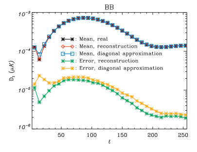
Figure 2: Comparison of the errors of the pseudo-$C_{\ell}$ estimator (green) and its diagonal approximation (yellow) when reconstructing the fullsky BB-spectrum (no lensing) from the real B-map with partial sky coverage. Generally speaking, at $\ell\approx 100$, both of them are unbiased. The pseudo-$C_{\ell}$ estimator is evidently better, but the ability to reduce the error is only by 20–30%.

$$\Delta(\ell)_{\rm{min}} \approx \sqrt{\left(\frac{\Delta_{1}(\ell)}{1.3k}\right)^{2}+\left(\frac{\Delta_{2}(\ell)}{2.5}\right)^{2}+\Delta_{c}^{2}(\ell)},$$ (4.1)

where 100 simulations are run for each test in figure 3–6. $\Delta_{1}(\ell)$ is the 1$\sigma$ error of the EB-leakage correction using the recycling method, as shown by the blue line in figure 1. As one can see in figure 1, a dedicated correction using the BUE can reduce $\Delta_{1}(\ell)$ roughly by factor 1.3. However, the difference between the BUE B-map and the real B-map (the pixel domain error) is non-Gaussian and non-isotropic, thus $\Delta_{1}(\ell)$ cannot benefit from the later fisher estimation of the fullsky spectrum, and will only passively receive the impact of fisher estimation. Because the leading order approximation of the fisher estimation (for $\ell$ around 100) is to multiply with $1/k$, the contribution of the residual EB-leakage error after applying the fisher estimator can be roughly estimated as $\Delta_{1}(\ell)/(1.3k)$. $\Delta_{2}(\ell)$ is the 1$\sigma$ error of recovering the full sky BB-spectrum using diagonal approximation on the real B-map with partial sky coverage (e.g., the yellow line in figure 2). Similarly, by using the dedicated fisher estimator, $\Delta_{2}(\ell)$ can be suppressed by factor 2.5 at $\ell\approx 100$. The relative strength of $\Delta_{1}(\ell)$ and $\Delta_{2}(\ell)$ is determined by the level of $r$ and the sky fraction. When only $r$ decreases, $\Delta_{1}(\ell)$ will not change, because it is dominated by the EE-spectrum; however, $\Delta_{2}(\ell)$ will decrease, because for the fisher estimator, the amplitude of error roughly follows the amplitude of the true spectrum. When only $f_{sky}$ increases, both $\Delta_{1}(\ell)$ and $\Delta_{2}(\ell)$ will decrease, because when more sky becomes available, all errors will decrease. For example, at the recombination peak ($\ell\simeq 100$), when $r=10^{-2}$ and $f_{sky}=10\%$, the term with $\Delta_{2}(\ell)$ is dominating; when $r=10^{-3}$ and $f_{sky}=2\%$, the two terms are comparable; but when $r=10^{-4}$ and $f_{sky}=2\%$, the term with $\Delta_{1}(\ell)$ is dominating. Lastly, $\Delta_{c}(\ell)$ is the cosmic variance, which is intrinsic and fixed. Therefore, $\Delta(\ell)_{\rm{min}}$ is a rough estimate of the minimal error compared to the theoretical BB-spectrum, which represents the maximum ability to detect the CMB B-mode.

Amongst various shapes of the mask, the disc mask has best symmetry, which helps to alleviate the EB-leakage. Thus disc masks with cosine apodizations are used for tests. Let’s consider the cases when the disc masks have $f_{sky}=$ 1%, 3%, 5%, 7%, 10% and 20%; and the apodization parameters are $a$ = 0.1, 0.3, $\cdots$, 0.9, where $a$ is the ratio between the apodization width and the disc radius, so high $a$-value means more aggressive apodization. The results are presented in figures 3–6 for $r=10^{-5}$, $10^{-4}$, $10^{-3}$ and ${10^{-2}}$, respectively. Note that in order to focus on a $5\sigma$ detection, the errors (colored lines) are amplified by factor 5, so by a simple comparison with the theoretical BB-spectrum (black line), one can easily see whether or not a $5\sigma$ detection is possible. Meanwhile, since an aggressive apodization will significantly reduce the signal-to-noise ratio, a detection is promising only when most of the colored lines are lower than the black line, so less aggressive apodizations are allowed.

The main results of this section are given in figures 3–6. Additionally, for convenience of reading, based on these figures, brief comments are given for the detectability of $r$ in Table 1 for various values of $f_{sky}$, e.g., the BICEP2 observation region has $f_{sky}\approx 1.2\%$. The meaning of the words in Table 1 are listed below:

1. “Impossible”: The specified $f_{sky}$ can hardly satisfy the requirement of detection.

2. “Barely”: The specified $f_{sky}$ can marginally satisfy the requirement of detection, but there is little room for other errors.

3. “Possible”: The specified $f_{sky}$ can satisfy the requirement of detection, and there is also room for other errors.

4. “Hopeful”: The specified $f_{sky}$ can satisfy the requirement of detection, and there is considerable room for other errors.

	$r=10^{-5}$	$r=10^{-4}$	$r=10^{-3}$	$r=10^{-2}$
$f_{sky}=0.01$	Impossible	Impossible	Barely	Possible
$f_{sky}=0.03$	Barely	Barely	Possible	Hopeful
$f_{sky}=0.05$	Barely	Possible	Hopeful	Hopeful
$f_{sky}=0.07$	Barely	Hopeful	Hopeful	Hopeful
$f_{sky}=0.10$	Possible	Hopeful	Hopeful	Hopeful
$f_{sky}=0.20$	Hopeful	Hopeful	Hopeful	Hopeful

Table 1: Rough comments on the possibility of detecting the CGWB at $5\sigma$ significance with various mask sizes. Based on figures 3–6. Note that perfect foreground removal, noise reduction, systematics control and delensing are assumed, thus this table shows the ultimate ability of detection.

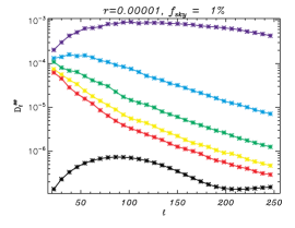
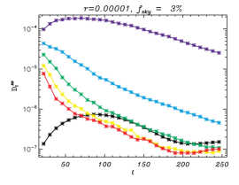
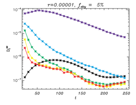
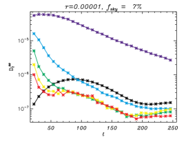
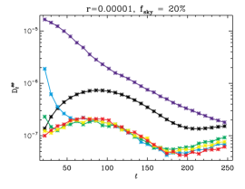
Figure 3: The lower limits of the error of detecting the CMB B-mode (colored lines). Note that they are amplified by factor 5 to show the threshold of $5\sigma$ detection. The colors corresponds to 10% – 90% (deep purple to red) apodizations. The theoretical BB-spectrum of $r=10^{-5}$ without lensing is shown by the black line for comparison. From top-left to bottom-right: $f_{sky}=$ 0.01, 0.03, 0.05, 0.07, 0.10 and 0.20. Perfect foreground removal, noise reduction, systematics control and delensing are assumed, so this is the absolutely unavoidable error attached to each choice of mask size and apodization strength.

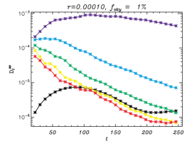
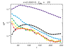
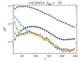
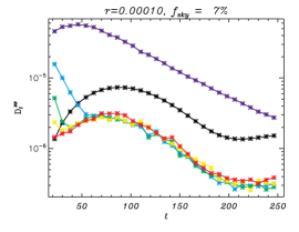
Figure 4: Similar to Figure 3 but for $r=10^{-4}$.

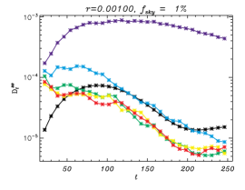
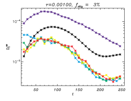
Figure 5: Similar to Figure 3 but for $r=10^{-3}$.

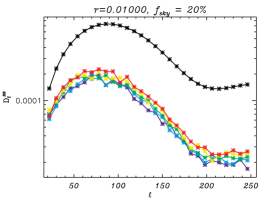
Figure 6: Similar to Figure 3 but for $r=10^{-2}$.

5 Summary and discussion

In summary, the general solution of the leakage due to data missing is given for integral transforms, and is used to estimate the maximum ability to detect the CGWB through the CMB with incomplete sky coverage. The results are presented in Figures 3–6, and for convenience of understanding, a brief outlook based on these figures is summarized in Table 1.

The price to use a prior estimator is to lose some generality. Theoretically speaking, it is possible to avoid this price by a brute force or MCMC exploration of all possible prior EE-spectra, and to find the one that gives the smallest error bars. However, this means to pay another incredibly huge price for the computational cost, which is not a good deal. In reality, since an excellent EE-spectrum was already given by the Planck mission with full sky surveys [7, 14], it is evidently a good idea to use this EE-spectrum as the prior information in the problem of the EB-leakage.

The BUE in this work has a great advantage that it can easily accommodate all kinds of prior information/constraints, even if they are non-Gaussian or non-analytic, e.g., realistic beam profile, systematics, lensing effects, etc. The only requirement is that the corresponding effects can be simulated and accommodated in $\{f_{i}(\bm{p})\}_{\mathcal{I}}$. An example of such simulations is the set of Planck full focal plane (FFP) simulations [15]. Meanwhile, any improvement of the prior information will immediately help to improve the overall estimation.

Interestingly, as shown by Fig. 1, for pure CMB signal, the error bars of the recycling method [3] are roughly only $30\%$ bigger than the ideal error bars, thus the result of the recycling method is an excellent approximation of the BUE, especially when computed at a higher resolution. However, as mentioned above, this must be further tested if non-Gaussian and non-analytic prior information is taken into account.

Finally, according to Table 1, to detect $r=10^{-3}\sim 10^{-2}$, it is recommended to use at least $f_{sky}=3\%$, and for $r=10^{-5}\sim 10^{-4}$, it is recommended to use $f_{sky}=10\%$ or more.

Appendix A Least square fitting of multi-variants

Given an ensemble of real data sets $\{H^{i}_{\xi}\}$ and an ensemble of corresponding measurements $\{h^{i}_{\xi}\}$, where $i$ denotes the index of the ensemble members, and $\xi$ denotes the index of data points within each member. Assume an estimation of $H_{\xi}$ is given by

$$H_{\xi}\approx\widetilde{H}_{\xi}=\sum_{\xi^{\prime}}\bm{M_{\xi\xi^{\prime}}}h_{\xi^{\prime}},$$ (A.1)

then the error of estimation at each point is

$$\begin{split}\delta_{\xi}^{2}&=\sum_{i}{|H_{\xi}^{i}-\widetilde{H}^{i}_{\xi}|^{2}}=\sum_{i}{|H_{\xi}^{i}-\sum_{\xi^{\prime}}\bm{M_{\xi\xi^{\prime}}}h^{i}_{\xi^{\prime}}|^{2}}.\end{split}$$ (A.2)

The minimal variance condition shows

$$\begin{split}\Delta=\sum_{\xi}\delta_{\xi}^{2}=\sum_{i,\xi}{|H_{\xi}^{i}-\sum_{\xi^{\prime}}\bm{M_{\xi\xi^{\prime}}}h^{i}_{\xi^{\prime}}|^{2}}=\min,\end{split}$$ (A.3)

thus

$$\begin{split}\frac{\partial\Delta}{\partial\bm{M_{\xi\xi^{\prime}}}}=&-2\sum_{i}{[H_{\xi}^{i}-\sum_{\xi^{\prime\prime}}{\bm{M}_{\xi\xi^{\prime\prime}}h_{\xi^{\prime\prime}}^{i}}]h^{i*}_{\xi^{\prime}}}=0\\ =&\sum_{i}{H^{i}_{\xi}h^{i*}_{\xi^{\prime}}}-\sum_{\xi^{\prime\prime}}{\bm{M}_{\xi\xi^{\prime\prime}}\sum_{i}{h^{i}_{\xi^{\prime\prime}}h^{i*}_{\xi^{\prime}}}},\end{split}$$ (A.4)

where $*$ denotes the complex conjugate. We write

$$\bm{P}_{\xi\xi^{\prime}}=\sum_{i}{H^{i}_{\xi}h^{i*}_{\xi^{\prime}}}$$ (A.5)

$$\bm{Q}_{\xi\xi^{\prime}}=\sum_{i}{h^{i}_{\xi}h^{i*}_{\xi^{\prime}}},$$

where $\bm{P}_{\xi\xi^{\prime}}$ is the cross covariance matrix between $H_{\xi}$ and $h_{\xi}$, and $\bm{Q}_{\xi\xi^{\prime}}$ is the covariance matrix of $h_{\xi}$. Thus equation (A.4) becomes:

$$\begin{split}\bm{P}=\bm{M}\bm{Q},\end{split}$$ (A.6)

and the coupling matrix that gives the BUE is

$$\begin{split}\bm{M}=\bm{P}\bm{Q^{-1}}.\end{split}$$ (A.7)

Note that this solution is also a general one: if $\bm{Q}$ is the covariance matrix of the known variable, $\bm{P}$ is the cross covariance matrix between the unknown and known variable, and the equation of estimation is linear, then the BUE of the unknown variable is given by eq. (A.7).

Appendix B Equivalence between the Fisher estimator and the maximum likelihood estimator

Here we provide a step-by-step proof that, for a Gaussian isotropic signal like the CMB, the Fisher estimator and the standard maximum likelihood estimator (e.g. [6]) give identical results.

The likelihood of a multi-variant Gaussian field $\bm{X}=\{x_{1},x_{2},\cdots\}$ that can be described by a set of model parameters $\bm{\Theta}=\{\theta_{1},\theta_{2},\cdots\}$ is:

$$L(\bm{X}|\bm{\Theta})\propto\frac{e^{-\frac{1}{2}\bm{X}^{T}C^{-1}\bm{X}}}{\sqrt{|C|}},$$ (B.1)

where $|C|$ means to take the determinant, and $C_{ij}=\langle x_{i}x_{j}\rangle$ is the covariance matrix in the pixel domain, determined by $\bm{\Theta}$. The above equation itself does not require isotropy, but by assuming isotropy, $\bm{\Theta}$ can be simplified to $\bm{\Theta}\equiv C_{\ell}$, the angular power spectrum, so the covariance matrix has the following form:

$$C_{ij}=\frac{1}{4\pi}\sum_{\ell}{(2l+1)W_{\ell}^{2}C_{\ell}P_{\ell}[\cos{(\theta_{ij})}]},$$ (B.2)

where $W_{\ell}$ is the beam profile, $P_{\ell}$ is the Legendre polynomial of order $l$, and $\theta_{ij}$ is the angle between pixel $i$ and $j$.

With eq. (B.2), the partial derivative of $C$ is:

$$\frac{\partial C}{\partial C_{\ell}}=\frac{1}{4\pi}(2\ell+1)W_{\ell}^{2}P_{\ell}[\cos{(\theta_{ij})}]=\rm{const}$$ (B.3)

The standard form of Fisher estimator for CMB is:

$$F_{\ell\ell^{\prime}} = 2\textbf{Tr}[CE^{\ell}CE^{\ell^{\prime}}]$$ (B.4)

$$\widetilde{C_{\ell}} = F_{\ell\ell^{\prime}}^{-1}y_{\ell^{\prime}}$$

where $F_{\ell\ell^{\prime}}$ is the Fisher matrix, and

$$E^{\ell}=\frac{1}{2}C^{-1}\frac{\partial C}{\partial C_{\ell}}C^{-1},\,y_{\ell}=\bm{X}^{T}E^{\ell}\bm{X}$$ (B.5)

Therefore, we should start from Equation B.1 and obtain Equation B.4.

For Equation B.1 to get its maximum, we have

$$\frac{\partial{\log{L}}}{\partial{C_{\ell}}}=0,$$ (B.6)

thus

$$-\bm{X}^{T}\frac{\partial C^{-}1}{\partial C_{\ell}}\bm{X}=\frac{1}{|C|}\frac{\partial|C|}{\partial C_{\ell}}.$$ (B.7)

Since

$$\frac{\partial}{\partial{C_{\ell}}}(CC^{-1})=0,$$

we have

$$\frac{\partial{C}}{\partial{C_{\ell}}}C^{-1}+C\frac{\partial{C^{-1}}}{\partial{C_{\ell}}}=0,$$ (B.8)

which means

$$\frac{\partial{C^{-1}}}{\partial{C_{\ell}}}=-C^{-1}\frac{\partial{C}}{\partial{C_{\ell}}}C^{-1},$$ (B.9)

so Equation B.7 becomes

$$\bm{X}^{T}C^{-1}\frac{\partial{C}}{\partial{C_{\ell}}}C^{-1}\bm{X}=\frac{1}{|C|}\frac{\partial|C|}{\partial C_{\ell}}.$$ (B.10)

With the definition of $y_{\ell}$, the above is shorted as

$$2y_{\ell}=\frac{1}{|C|}\frac{\partial|C|}{\partial C_{\ell}}.$$ (B.11)

For the right hand side, the variation of $C$ is

$$C+\frac{\partial{C}}{\partial{C_{\ell}}}dC_{\ell}=Ck,$$ (B.12)

so

$$k=I+C^{-1}\frac{\partial{C}}{\partial{C_{\ell}}}dC_{\ell},$$ (B.13)

where $I$ is the unitary matrix. According to the definition of determinant,

$$d|C|=|Ck|-|C|=|C|\,|k|-|C|=|C|\,\textbf{Tr}\left(C^{-1}\frac{\partial{C}}{\partial{C_{\ell}}}\right)dC_{\ell}.$$ (B.14)

Thus

$$\frac{1}{|C|}\frac{\partial{|C|}}{\partial{C_{\ell}}}=\textbf{Tr}\left(C^{-1}\frac{\partial{C}}{\partial{C_{\ell}}}\right)$$ (B.15)

Substitute into Equation B.11 gives

$$y_{\ell}=\frac{1}{2}\textbf{Tr}\left(C^{-1}\frac{\partial{C}}{\partial{C_{\ell}}}\right).$$ (B.16)

For Gaussian field, $y_{\ell}$ is linear function of $C_{\ell}$, thus

$$\begin{split}y_{\ell}&=\sum_{\ell^{\prime}}\frac{\partial y_{\ell}}{\partial{C_{\ell^{\prime}}}}C_{\ell^{\prime}}\\ \frac{\partial y_{\ell}}{\partial C_{\ell^{\prime}}}&=F_{\ell\ell^{\prime}}=\frac{1}{2}\frac{\partial\textbf{Tr}(C^{-1}\frac{\partial{C}}{\partial{C_{\ell}}})}{\partial C_{\ell^{\prime}}}.\end{split}$$ (B.17)

Using Equation B.8, and considering that $\partial{C}/\partial{C_{\ell}}$ is constant and $C$ is symmetric, we get

$$\begin{split}F_{\ell\ell^{\prime}}&=\frac{\partial y_{\ell}}{\partial C_{\ell^{\prime}}}\\ &=\frac{1}{2}\textbf{Tr}\left[\frac{\partial C^{-1}}{\partial C_{\ell^{\prime}}}\frac{\partial{C}}{\partial{C_{\ell}}}\right]\\ &=\frac{1}{2}\textbf{Tr}\left[C^{-1}\frac{\partial C}{\partial C_{\ell^{\prime}}}C^{-1}\frac{\partial C}{\partial C_{\ell}}\right]\\ &=2\textbf{Tr}[CE^{\ell}CE^{\ell^{\prime}}],\end{split}$$

which returns exactly to Equation B.4. Therefore, for a Gaussian isotropic signal like the CMB, the Fisher estimator and maximum likelihood estimator are identical.

References

- [1] A. Lewis, A. Challinor and N. Turok, Analysis of CMB polarization on an incomplete sky, Phys. Rev. D 65 (Jan., 2001) 023505, [astro-ph/0106536].
- [2] E. F. Bunn, M. Zaldarriaga, M. Tegmark and A. de Oliveira-Costa, E/B decomposition of finite pixelized CMB maps, Phys. Rev. D67 (2003) 023501, [astro-ph/0207338].
- [3] H. Liu, J. Creswell, S. von Hausegger and P. Naselsky, Methods for pixel domain correction of EB leakage, arXiv e-prints (Nov, 2018) arXiv:1811.04691, [1811.04691].
- [4] H. Liu, J. Creswell and K. Dachlythra, Blind correction of the EB-leakage in the pixel domain, Journal of Cosmology and Astroparticle Physics 2019 (apr, 2019) 046–046, [1904.00451].
- [5] M. Tegmark, How to measure CMB power spectra without losing information, Phys. Rev. D 55 (May, 1997) 5895–5907, [astro-ph/9611174].
- [6] L. Verde, H. V. Peiris, D. N. Spergel, M. R. Nolta, C. L. Bennett, M. Halpern et al., First-Year Wilkinson Microwave Anisotropy Probe (WMAP) Observations: Parameter Estimation Methodology, Astrophys. J.Suppl. 148 (Sept., 2003) 195–211, [astro-ph/0302218].
- [7] Planck Collaboration, R. Adam, P. A. R. Ade, N. Aghanim, Y. Akrami, M. I. R. Alves et al., Planck 2015 results. I. Overview of products and scientific results, Astr. Astrophys. 594 (Sept., 2016) A1, [1502.01582].
- [8] Planck Collaboration, N. Aghanim, M. Arnaud, M. Ashdown, J. Aumont, C. Baccigalupi et al., Planck 2015 results. XI. CMB power spectra, likelihoods, and robustness of parameters, Astr. Astrophys. 594 (Sept., 2016) A11.
- [9] M. Tegmark and A. de Oliveira-Costa, How to measure CMB polarization power spectra without losing information, Phys. Rev. D 64 (Sept., 2001) 063001, [astro-ph/0012120].
- [10] D. Molinari, A. Gruppuso, G. Polenta, C. Burigana, A. De Rosa, P. Natoli et al., A comparison of CMB angular power spectrum estimators at large scales: the TT case, Mon. Not. R. Astr. Soc. 440 (May, 2014) 957–964, [1403.1089].
- [11] E. Hivon, K. M. Górski, C. B. Netterfield, B. P. Crill, S. Prunet and F. Hansen, MASTER of the Cosmic Microwave Background Anisotropy Power Spectrum: A Fast Method for Statistical Analysis of Large and Complex Cosmic Microwave Background Data Sets, Astrophys. J. 567 (Mar., 2002) 2–17, [astro-ph/0105302].
- [12] J. B. Jewell, H. K. Eriksen, B. D. Wandelt, I. J. O’Dwyer, G. Huey and K. M. Górski, A Markov Chain Monte Carlo Algorithm for Analysis of Low Signal-To-Noise Cosmic Microwave Background Data, Astrophys. J. 697 (May, 2009) 258–268, [0807.0624].
- [13] A. Gruppuso, A. de Rosa, P. Cabella, F. Paci, F. Finelli, P. Natoli et al., New estimates of the CMB angular power spectra from the WMAP 5 year low-resolution data, Mon. Not. R. Astr. Soc. 400 (Nov., 2009) 463–469, [0904.0789].
- [14] Planck Collaboration, Y. Akrami, F. Arroja, M. Ashdown, J. Aumont, C. Baccigalupi et al., Planck 2018 results. I. Overview and the cosmological legacy of Planck, ArXiv e-prints (July, 2018) , [1807.06205].
- [15] Planck Collaboration, P. A. R. Ade, N. Aghanim, M. Arnaud, M. Ashdown, J. Aumont et al., Planck 2015 results. XII. Full focal plane simulations, Astr. Astrophys. 594 (Sept., 2016) A12, [1509.06348].
- [16] K. M. Górski, E. Hivon, A. J. Banday, B. D. Wandelt, F. K. Hansen, M. Reinecke et al., HEALPix: A Framework for High-Resolution Discretization and Fast Analysis of Data Distributed on the Sphere, Astrophys. J. 622 (Apr., 2005) 759–771, [astro-ph/0409513].