Dynamic time series clustering via volatility change-points

Abstract

This note outlines a method for clustering time series based on a statistical model in which volatility shifts at unobserved change-points. The model accommodates some classical stylized features of returns and its relation to GARCH is discussed. Clustering is performed using a probability metric evaluated between posterior distributions of the most recent change-point associated with each series. This implies series are grouped together at a given time if there is evidence the most recent shifts in their respective volatilities were coincident or closely timed. The clustering method is dynamic, in that groupings may be updated in an online manner as data arrive. Numerical results are given analyzing daily returns of constituents of the S&P 500.

1 Introduction

The purpose of this note is to outline, contextualize and demonstrate a method for clustering time series using a change-point model. The emphasis is on conveying the ideas of the method rather than depth or generality, although some possible extensions and research directions are given at the end in section 4. A Python implementation in the form of a Jupyter notebook is available: https://github.com/nckwhiteley/volatility-change-points.

1.1 Time series clustering

Time series clustering is typically a two-step procedure. The first step is to specify a pairwise measure of dissimilarity between series. An overview of several popular approaches is given in (Montero et al., 2014, Sec. 2). To mention just a few examples, this dissimilarity could be derived from fairly simple statistics, such as cross-correlation; could involve solving an optimization problem to find a ‘best’ match between each pair of series, for instance using the Fréchet distance or Dynamic Time Warping (Berndt and Clifford, 1994); or could involve fitting a some form of model to each of the series, then computing a distance between the fitted parameter values (Corduas and Piccolo, 2008; Otranto, 2008) or forecast distributions (Alonso et al., 2006; Vilar et al., 2010).

The second step is to pass the dissimilarity measure to an algorithm which determines associations between the series. Again to mention just a few popular techniques, hierarchical methods such as agglomerative clustering, see for example (Murphy, 2012, Sec. 25.5) for an overview, form clusters sequentially. Each datum starts in its own cluster and pairs of clusters are merged step-by-step in accordance with some linkage criterion which quantifies how between-cluster dissimilarity is derived from between-series dissimilarity. Centroid-based techniques such as $k$-means (MacQueen, 1967) or its generalizations beyond Euclidean distance to, e.g., Bregman divergences (Banerjee et al., 2005) or Wasserstein distances (Ye et al., 2017) choose a collection of cluster centers to minimize the sum of within-cluster divergences/distances. The computational cost of global minimization is usually prohibitive and so for implementation one settles for a local minimum obtained using an iterative refinement method, such as Lloyd’s algorithm (Lloyd, 1982) in the case of Euclidean distance.

A further level of sophistication is to approach clustering as a statistical inference problem, with associations between data points and clusters treated as latent variables to be inferred under a probabilistic model. This allows uncertainty over clusterings, model parameters and model structure to be quantified and reported in a principled manner. The price to pay is usually an increased computational cost, for example incurred through the EM algorithm, variational methods or Monte Carlo sampling. The question of how to scale-up these methods to tackle large data sets is an active topic of research. For a recent overview and ideas involving parallelization and multi-step procedures, see (Ni et al., 2018).

We propose a method which may be regarded as a half-way point between a full-blown statistical treatment of time series clustering and the simple two-step recipe described above. We do not perform probabilistic modeling of associations, but we do perform probabilistic modeling on a per-series basis and use it to define a notion of dissimilarity.

1.2 Financial time series clustering

Clustering of time series can serve a variety of purposes. In exploratory data analysis one may simply want to discover groupings or unexpected phenomena, and then summarize or report them for purposes of dimension reduction or interpretation. Clustering may be one ingredient within a broader statistical workflow, in which actions or decisions are taken on the basis of discovered clusters.

Stemming from an influential paper of Mantegna (1999), clustering of financial time series using dissimilarity measures derived from correlation has been applied to assist fundamental understanding of markets, risk management, portfolio optimization and trading. A comprehensive overview of research on this topic across machine learning, econophysics, statistical physics, econometrics and behavioral finance is maintained on arXiv by Marti et al. (2017). The current version includes a bibliography of over 400 references which we shall not attempt to summarize.

An alternative approach to time series clustering, which does not feature in (Marti et al., 2017), is to define dissimilarity by some distance between parameter vectors obtained by fitting a model to each of the series individually. Otranto (2008) gives a detailed account of dissimilarity measures in this vein, and uses Wald tests and autoregressive metrics to measure the distance between GARCH processes and thus cluster based on the heteroskedastic characteristics. Otranto (2010) extends this technique to clustering based on distance between fitted Dynamic Conditional Correlation models, and deploys the resulting covariance matrix estimates within portfolio optimization.

As discussed by Marti et al. (2016) and Marti et al. (2017, Sec 4), a research topic still in its infancy but of considerable interest is how to track changes in market structure, by recognizing clusters which may change over time. Indeed Marti et al. (2017, Sec 4) report that many empirical studies do not achieve this but just deliver a static clustering based all data available for a given time period. An obvious step towards dynamic clustering is to apply a static clustering method on a sliding window. If, for example, the clustering techniques of Otranto (2008, 2010) were applied in this manner, the length of the window would achieve a trade-off between temporal locality and noisy parameter estimates, hence noisy estimates of dissimilarity. The question of how long the window should be in order to best deal with time-varying clusters is often not an easy one to answer rigorously.

The method introduced below defines dissimilarity between time series not in terms of correlation or parameter estimates, but rather in terms of evidence about times of volatility change-points. As a consequence, time series which evidence shifts in volatility around the same points in times tend to be clustered together. This is of interest because synchrony in volatility change-points across series may arise from common underlying market factors or similar responses to changing market conditions which the method may help to uncover. One appealing feature of the method is that it naturally accommodates dynamic clustering, in the sense that clusters can be re-evaluated at each point in time as new data arrive, but it circumvents the need to work on a sliding window: the underlying change-point model effectively adapts to the time-scale of volatility changes of each series.

2 The change-point model and dissimilarity measure

2.1 A generic change-point model for a single time series

Consider a sequence of unobserved, integer valued and strictly increasing change-points $(T_{n})_{n\in\mathbb{N}_{0}}$. $T_{0}$ is equal to zero with probability one, and the increments $(T_{n}-T_{n-1})_{n\geq 1}$ are i.i.d. with c.d.f. denoted by $G$.

For $t\in\mathbb{N}_{0}$, define $N(t)\coloneqq\sup\{n\geq 0:T_{n}<t\}$, $\tau_{t}\coloneqq T_{N(t)}$ and observe that $(\tau_{t})_{t\geq 1}$ is a Markov chain, with transition probabilities:

$$p(\tau_{t+1}=s|\tau_{t}=u)=\begin{cases}\frac{G(t-u)-G(t-1-u)}{1-G(t-1-u)},&s=t,\\ \frac{1-G(t-u)}{1-G(t-1-u)},&s=u\in\{0,\ldots,t-1\},\\ 0,&\mathrm{otherwise},\end{cases}$$ (1)

corresponding to whether a new change-point has occurred or not.

Let $(y_{t})_{t\in\mathbb{N}_{0}}$ be observed returns which are assumed to be jointly distributed with $(\tau_{t})_{t\geq 1}$ such that for each $t\geq 1$,

$$p(\tau_{1:t},y_{0:t})=p(y_{0})\prod_{s=1}^{t}p(\tau_{s}|\tau_{s-1})p(y_{s}|\tau_{s},y_{0:s-1}),$$ (2)

with the convention $p(\tau_{1}|\tau_{0})\equiv\delta_{0}(\tau_{1})$, the Kronecker delta at $0$, to respect the fact that $T_{0}$ is zero with probability $1$.

Consider the sequence of probability mass functions $(\pi_{t})_{t\geq 1}$,

$$\pi_{t}(s)\coloneqq p(\tau_{t}=s|y_{0:t}).$$ (3)

Again due to the fact that $T_{0}$ is zero with probability $1$, we have $\pi_{1}(0)=1$. Combining the conditional independence structure of (2) with (1), elementary marginalization and Bayes’ rule validate the following recursion, for $t\geq 1$,

$$\pi_{t+1}(s)\propto\begin{cases}p(y_{t+1}|\tau_{t+1}=t,y_{0:t})\sum_{u=0}^{t-1}\left[\frac{G(t-u)-G(t-1-u)}{1-G(t-1-u)}\pi_{t}(u)\right],&s=t,\\ p(y_{t+1}|\tau_{t+1}=s,y_{0:t})\frac{1-G(t-s)}{1-G(t-1-s)}\pi_{t}(s),&s\in\{0,\ldots,t-1\},\\ 0,&\mathrm{otherwise}.\end{cases}$$ (4)

This change-point model and the recursion (4) are directly inspired by those of Chopin (2007), Fearnhead and Liu (2007) and Adams and MacKay (2007). Our model is slightly more general than those of Fearnhead and Liu (2007) and Adams and MacKay (2007), who assumed that conditional on a change-point time, observations after that time are independent of observations before. Note (2) does not imply such independence.

In section 2.4 we describe an instance of the above change-point model in which the terms $p(y_{t+1}|\tau_{t+1},y_{0:t})$ arise by analytically integrating out parameters associated with the change-points under conjugate prior distributions. This makes our setting more restrictive than that of Chopin (2007), who did not assume such analytic integration possible, but instead used numerical integration in the form of a sequential Monte Carlo algorithm.

2.2 The dissimilarity measure

Suppose now that one is presented with $m\geq 1$ series of returns $\{(y_{t}^{i})_{t\in\in\mathbb{N}_{0}},i=1,\ldots,m\}$. Let $\pi_{t}^{i}$ be as in (3) with $(y_{t})_{t\in\in\mathbb{N}_{0}}$ there replaced by $(y_{t}^{i})_{t\in\in\mathbb{N}_{0}}$. We propose to cluster the series at any given time $t$ with dissimilarity taken to be a probability metric evaluated between the distributions $\{\pi_{t}^{i},i=1,\ldots,m\}$. Thus series will be clustered at time $t$ if, through $\{\pi_{t}^{i},i=1,\ldots,m\}$, they exhibit similar evidence about the times of their respective most recent change-points.

Which probability metric to choose? It seems sensible to consider: i) interpretation and ii) computational overhead. To address the first of these two criteria, consider the total variation distance:

$$\mathrm{TV}(\pi^{1},\pi^{2})=\frac{1}{2}\sum_{s\in\mathbb{N}_{0}}|\pi^{1}(s)-\pi^{2}(s)|.$$

The total variation distance is maximal and equal to $1$ as soon as $\pi^{1}$ and $\pi^{2}$ have disjoint support, which is a rather restrictive notion of dissimilarity. For instance, for two Kronecker delta’s $\pi^{1}=\delta_{t}$ and $\pi^{2}=\delta_{t+s}$,

$$\mathrm{TV}(\delta_{t},\delta_{t+s})=1,\quad\text{if}\quad|s|\neq 0.$$ (5)

For describing distributions over change-points this insensitivity to translation seems undesirable - a more appealing property might be that the distance is strictly increasing in $|s|$. Alternatives such as the Hellinger and $L_{2}$ distances involve similarly summing of point-wise differences between probability mass functions, or functions thereof, and hence have the same drawback. Divergences which involve ratios of probability mass functions such as $\chi^{2}$ or Kullback-Liebler similarly fail to express dissimilarity if the support of one mass function is not contained within that of the other.

The total variation distance can be regarded as one instance of a Wasserstein distance: given a distance $d(\cdot,\cdot)$ on $\mathbb{N}_{0}$ and $p\geq 1$, the $p$’th Wasserstein distance associated with $d$ is:

$$W_{p}(\pi^{1},\pi^{2})\coloneqq\left(\inf_{\gamma\in\Gamma(\pi^{1},\pi^{2})}\sum_{(s,t)\in\mathbb{N}_{0}\times\mathbb{N}_{0}}d(s,t)^{p}\gamma(s,t)\right)^{1/p},$$ (6)

where $\Gamma$ is the set of all probability mass functions on $\mathbb{N}_{0}\times\mathbb{N}_{0}$ whose marginals are $\pi^{1}$ and $\pi^{2}$. The total variation distance arises if one takes $d$ to be the discrete distance $d(s,t)=\mathbf{1}_{\{s\neq t\}}$ and $p=1$.

If instead $d$ is the usual distance on $\mathbb{N}_{0}$, $d(s,t)=|s-t|$, we have

$$W_{p}(\delta_{t},\delta_{t+s})=|s|,$$ (7)

and slightly more generally it can be shown by a direct computation of the infimum in (6) that:

$$W_{p}(a\delta_{s}+(1-a)\delta_{t},b\delta_{s}+(1-b)\delta_{t})=|a-b|^{1/p}|s-t|,$$ (8)

see (Bobkov and Ledoux, 2016, Ex 2.3). Whilst (7) and (8) are of course rather specific examples, they illustrate the manner in which the Wasserstein distance associated with $d(s,t)=|s-t|$ is more expressive than total variation distance regarding translation, and therefore arguably more suited to our purposes of comparing distributions over change-point times.

Turning to the criterion of computational overhead, in the case of $d(s,t)=|s-t|$ on $\mathbb{N}_{0}$, the Wasserstein distance is conveniently available in closed form:

$$W_{p}(\pi^{1},\pi^{2})=\left(\int_{0}^{1}|F_{1}^{-1}(v)-F_{2}^{-1}(v)|^{p}\mathrm{d}v\right)^{1/p}$$

where $F_{i}^{-1}(v)=\inf\{t\in\mathbb{N}_{0}:F_{i}(t)\geq v\}$ is the generalized inverse c.d.f. of $\pi^{i}$. Even more conveniently from a computational point of view, is the fact that:

$$W_{1}(\pi^{1},\pi^{2})=\sum_{s\in\mathbb{N}_{0}}|F_{1}(s)-F_{2}(s)|,$$ (9)

see (Bobkov and Ledoux, 2016) for background.

With these considerations we shall settle on (9) applied to each pair $\pi_{t}^{i},\pi_{t}^{j}$ as our dissimilarity measure at time $t$. Note that the support of any $\pi_{t}^{i}$ is always contained in $\{0,1,\ldots,t-1\}$. Moreover, if the approximation technique suggested in section 2.3 is applied, each approximating distribution $\hat{\pi}_{t}^{i}$ (more details later) will have a number of support points uniformly upper bounded in t, and hence the cost of evaluating $W_{1}(\hat{\pi}_{t}^{i},\hat{\pi}_{t}^{j})$ is uniformly upper bounded in $t.$

Choosing the dissimilarity measure completes the first of the two steps described in section 1. What options are available for the second step? Hierarchical clustering can be performed immediately after evaluating the pairwise distances and we shall illustrate this approach through numerical experiments. For a centroid-based approach in the style of $k$-means, one needs to introduce the notion of Wasserstein barycentre, which is the Fréchet mean in the space of probability distributions equipped with the Wasserstein distance. Computing these barycentres is a non-trivial task in general, see (Peyré and Cuturi, 2019) for numerical methods.

2.3 Online implementation

The number of terms in the summation in (4) clearly increases linearly with $t$. Hence the cost of computing this recursion from time zero up to some time $t$ is quadratic in $t$. A simple route towards an online algorithm, i.e. one whose computational cost per time step does not increase with time, is to introduce an approximation to each $\pi_{t}$ with a number of support points uniformly upper bounded in $t$.

For instance, consider a simple pruning strategy: fix a number of support points $n\geq 1$. For $t\leq n$, computer $\pi_{t}$ exactly using the recursion (4). For $t>n$ assume one already has an approximation to $\pi_{t}$, call it $\hat{\pi}_{t}$ which has $n$ support points in $\{0,\ldots,t-1\}$. Then one can substitute $\hat{\pi}_{t}$ for $\pi_{t}$ in the right hand side of (4), and retain the $n$ of the $n+1$ resulting support points associated with highest probabilities to give an approximation $\hat{\pi}_{t+1}$ to $\pi_{t+1}$.

A further consideration for online implementation of (4) is the cost of evaluating $p(y_{t+1}|\tau_{t+1},y_{0:t})$, does this also increase with $t$? In the instance of the change-point model described in section 2.4, we shall show that $p(y_{t+1}|\tau_{t+1},y_{0:t})$ depends on $y_{0:t}$ through statistics which can be updated online as data arrive, and hence it is possible to evaluate the terms $p(y_{t+1}|\tau_{t+1},y_{0:t})$ sequentially in $t$ at a fixed cost per time step.

2.4 A particular instance of the change-point model

Let $(T_{n})_{n\geq 0}$ be distributed as in section 2.1. We now introduce a specific model for the returns $(y_{t})_{t\geq 0}$ which, upon analytically marginalizing out certain parameters, will satisfy (2.1) with a closed-form expression for $p(y_{t+1}|\tau_{t+1},y_{0:t})$. In turn, this can be plugged into the recursion (4) or its approximation discussed in section 2.3, in order to evaluate the dissimilarity measure.

Consider a sequence of triples of parameters $(\mu_{n},\alpha_{n},\sigma_{n}^{2})_{n\in\mathbb{N}_{0}}$ and assume that:

$$y_{t}=\mu_{N(t)}+\alpha_{N(t)}y_{t-1}+\sigma_{N(t)}\epsilon_{t},$$ (10)

where $(\epsilon_{t})_{t\geq 1}$ are i.i.d. $\mathsf{N}(0,1)$. Thus $(\mu_{n},\alpha_{n},\sigma_{n}^{2})$ parameterize the conditional joint distribution of the data between the $n$’th and $(n+1)$’th change-points, i.e. $(y_{T_{n}+1},\ldots,y_{T_{n+1}})$, given $y_{T_{n}}$.

We assume the following prior independence properties: the sequence $(\mu_{n},\alpha_{n},\sigma_{n}^{2})_{n\geq 0}$ and the sequence $(T_{n})_{n\geq 0}$ are independent, and the triples $(\mu_{n},\alpha_{n},\sigma_{n}^{2})_{n\geq 0}$ are independent across $n$. It can be shown that as a consequence of these independences and (10),

$$p(y_{t+1}|\tau_{t+1}=s,y_{0:t}) =p(y_{t+1}|\tau_{t+1}=s,y_{s:t}),$$ (11)

$$p(\mu_{N(t)},\alpha_{N(t)},\sigma_{N(t)}^{2}|\tau_{t}=s,y_{0:t}) =p(\mu_{N(t)},\alpha_{N(t)},\sigma_{N(t)}^{2}|\tau_{t}=s,y_{s:t}).$$ (12)

The intuitive interpretation of these identities is that conditional on the time of the most-recent change-point being $s$, data strictly prior to $s$ are irrelevant to: predicting the next data point, as per (11), and inference for $\mu_{N(t)},\alpha_{N(t)},\sigma_{N(t)}^{2}$, i.e., the parameters associated with the most recent change-point, as per (12).

To arrive at a closed-form expression for $p(y_{t+1}|\tau_{t+1}=s,y_{s:t})$ we set a zero-mean Normal-Inverse-Gamma prior distribution on each parameter triple:

$$p(\mu_{n},\alpha_{n},\sigma_{n}^{2})=\frac{1}{2\pi|V_{0}|^{1/2}}\frac{b^{a}}{\Gamma(a)}\left(\frac{1}{\sigma_{n}^{2}}\right)^{a+2}\exp\left(-\frac{2b+\beta_{n}^{\mathrm{T}}V_{0}^{-1}\beta_{n}}{2\sigma_{n}^{2}}\right),$$ (13)

where $\beta_{n}\coloneqq[\mu_{n}\;\alpha_{n}]^{\mathrm{T}}$, $V_{0}\coloneqq\mathrm{diag(\delta_{0}^{2},\delta_{1}^{2})},$ and $a,b,\delta_{0},\delta_{1}$ are hyper-parameters which are common across $n$.

The following proposition gives the expression for $p(y_{t+1}|\tau_{t+1}=s,y_{s:t})$ as desired, and marginal posterior densities for the parameters $\beta_{N(t)}$ and $\sigma_{N(t)}^{2}$ conditional on the time of the most recent change-point.

Proposition 1.

$$p(y_{t+1}|\tau_{t+1}=s,y_{s:t})=\mathsf{St}\left(2a_{s,t},h_{t+1}w_{s,t},\frac{b_{s,t}}{a_{s,t}}(1+h_{t+1}V_{s,t}h_{t+1}^{\mathrm{T}})\right),$$ (14)

$$p(\beta_{N(t)}|\tau_{t}=s,y_{s:t})=\mathsf{St}\left(2a_{s,t},w_{s,t},\frac{b_{s,t}}{a_{s,t}}V_{s,t}\right),$$ (15)

$$p(\sigma_{N(t)}^{2}|\tau_{t}=s,y_{s:t})=\mathsf{IG}(a_{s,t},b_{s,t}),$$ (16)

where

$$w_{s,t}\coloneqq V_{s,t}H_{s,t}^{T}y_{s+1:t},$$ (17)

$$V_{s,t}\coloneqq(V_{0}^{-1}+H_{s,t}^{\mathrm{T}}H_{s,t})^{-1},$$ (18)

$$a_{s,t}\coloneqq a+\frac{t-s}{2},$$ (19)

$$b_{s,t}\coloneqq b+\frac{1}{2}(\|y_{s+1:t}\|^{2}-w_{s,t}^{\mathrm{T}}V_{s,t}^{-1}w_{s,t}),$$ (20)

$H_{s,t}\coloneqq[h_{t}^{\mathrm{T}}\cdots h_{s+1}^{\mathrm{T}}]^{\mathrm{T}}$ , $h_{t}\coloneqq[1\;y_{t-1}]$, and $y_{s+1:t}\equiv[y_{t}\;y_{t-1}\;\cdots\;y_{s+1}]^{\mathrm{T}}$.

Proof sketch..

Note from (10),

$$y_{\tau_{t}+1:t}=\left[\begin{array}[]{c}y_{t}\\ \vdots\\ y_{\tau_{t}+1}\end{array}\right]=H_{\tau_{t},t}\beta_{N(t)}+\sigma_{N(t)}\left[\begin{array}[]{c}\epsilon_{t}\\ \vdots\\ \epsilon_{\tau_{t}+1}\end{array}\right].$$

The expressions in (14)-(16) can therefore be obtained by conditioning on $\tau_{t+1}=s$ or $\tau_{t}=s$, and then applying standard results for Bayesian linear regression under a Normal-Inverse-Gamma prior, see for example (Murphy, 2012, Sec 7.6.3). ∎

Further to the considerations in section 2.3 it is important to notice that $(w_{s,t})_{t>s}$, $(V_{s,t})_{t>s}$, $(a_{s,t})_{t>s}$, $(b_{s,t})_{t>s}$ can be calculated in a recursive manner, so that the cost of evaluating each term of the form $p(y_{t+1}|\tau_{t+1},y_{0:t})$, $p(y_{t+2}|\tau_{t+2},y_{0:t+1})$, etc. does not increase with $t$. The following lemma gives the details.

Lemma 2.

For fixed $s\geq 0$,

$$V_{s,s+1} =(V_{0}^{-1}+h_{s+1}^{\mathrm{T}}h_{s+1})^{-1}, V_{s,t+1} =V_{s,t}-\frac{V_{s,t}h_{t+1}^{\mathrm{T}}h_{t+1}V_{s,t}}{1+h_{t+1}V_{s,t}h_{t+1}^{\mathrm{T}}},$$

$$\tilde{y}_{s,s+1} =y_{s+1}h_{s+1}^{\mathrm{T}}, \tilde{y}_{s,t+1} =\tilde{y}_{s,t}+y_{t+1}h_{t+1}^{\mathrm{T}},$$

$$\|y_{s+1:s+1}\|^{2} =y_{s+1}^{2}, \|y_{s+1:t+1}\|^{2} =\|y_{s+1:t}\|^{2}+y_{t+1}^{2},$$

$$a_{s,s+1} =a+\frac{1}{2}, a_{s,t+1} =a_{s,t}+\frac{1}{2},$$

and for $t\geq s$,

$$w_{s,t}=V_{s,t}\tilde{y}_{s,t}.$$

Proof.

The expression for $V_{s,t+1}$ follows from

$$V_{s,t+1}^{-1}=V_{0}+H_{s,t+1}^{\mathrm{T}}H_{s,t+1}=V_{0}+H_{s,t}^{\mathrm{T}}H_{s,t}+h_{t+1}^{\mathrm{T}}h_{t+1}=V_{s,t}^{-1}+h_{t+1}^{\mathrm{T}}h_{t+1},$$

and the Sherman-Morrison formula. The other expressions are quite straight forward. ∎

2.5 Interpretation and relation to GARCH

It is widely recognized that returns data at daily or higher frequencies often exhibit certain stylized features:

1. long-run mean or median close to zero, and heavy tails;

2. long-run auto-correlation of returns which is small or decays quickly with lag-length, but auto-correlation of absolute or squared returns which decays slowly;

3. time-dependent volatility.

To explain the interpretation of the change-point model in this context, consider GARCH$(1,1)$:

$$y_{t} =\varsigma_{t}\epsilon_{t},$$ (21)

$$\varsigma_{t}^{2} =c_{0}+c_{1}y_{t-1}^{2}+\rho\varsigma_{t-1}^{2},$$ (22)

where $(\epsilon_{t})_{t\geq 0}$ is a white noise process. This is perhaps the most widely used time series model which accommodates the stylized features described above:

1. in the original presentation of Bollerslev (1986), $(\epsilon_{t})_{t\geq 0}$ were taken as i.i.d. standard Gaussian, so that the marginal distribution of $y_{t}$ under (21) is a scale-mixture of zero-mean Gaussians. To further account for heavy-tails, Bollerslev (1987) suggested instead a $t$-distribution centered at zero for $(\epsilon_{t})_{t\geq 0}$, with unit scale parameter;

2. due to the independence of the $(\epsilon_{t})_{t\geq 0}$ and the centering of their common distribution at zero, it is easily seen that the autocorrelation of $(y_{t})_{t\geq 0}$ (assuming it exists) is zero. The sequence of squared returns $y_{t}^{2}$ from GARCH$(1,1)$ is an ARMA process (Andersen et al., 2009, Thm 7, p.61) and hence may exhibit non-trivial autocorrelation;

3. time-dependent volatility is modelled through the ‘conditional-variance’ equation (22).

These properties manifest themselves in the predictive distributions $p(y_{t+1}|y_{0:t})$ associated with GARCH$(1,1)$; if indeed $(\epsilon_{t})_{t\geq 0}$ are unit scale and zero-centered student’s-$t$ variables with $2a$ degrees of freedom, then:

$$p(y_{t+1}|y_{0:t})=\mathsf{St}(2a,0,\varsigma_{t+1}^{2}),$$ (23)

where by writing out (22),

$$\varsigma_{t+1}^{2}=c_{0}\sum_{s=0}^{t}\rho^{s}+c_{1}\sum_{s=0}^{t}\rho^{s}y_{t-s}^{2}+\rho^{t+1}\varsigma_{0}^{2}.$$ (24)

Let us now explain the connection to (14). For purposes of exposition, suppose that the parameters $(\mu_{n})_{n\geq 0}$ are omitted from the change-point model, in the sense that (10) is simplified to:

$$y_{t}=\alpha_{N(t)}y_{t-1}+\sigma_{N(t)}\epsilon_{t},$$ (25)

and suppose the prior on each parameter pair $(\alpha_{n},\sigma_{n}^{2}$) is just the marginal prior of these two parameters under (13).

Proposition 3.

Omitting $(\mu_{n})_{n\geq 0}$ in the sense of (25) results in the following expression for (14):

$$p(y_{t+1}|\tau_{t+1}=s,y_{s:t})=\mathsf{St}(2a+t-s,\hat{\alpha}_{s,t}y_{t},\hat{\sigma}_{s,t}^{2}),$$ (26)

where

$$\hat{\alpha}_{s,t} \coloneqq\frac{\sum_{i=s}^{t-1}y_{i}y_{i+1}}{\delta_{1}^{-1}+\sum_{i=s}^{t-1}y_{i}^{2}},$$ (27)

$$\hat{\sigma}_{s,t}^{2} \coloneqq\left[(1-\hat{\alpha}_{s,t}^{2})\frac{\sum_{i=s}^{t-1}y_{i}^{2}}{2a+t-s}+\frac{2b+y_{t}^{2}-y_{s}^{2}-\delta_{1}^{-1}}{2a+t-s}\right]\left(1+\frac{y_{t}^{2}}{\delta_{1}^{-1}+\sum_{i=s}^{t-1}y_{i}^{2}}\right)$$ (28)

Before giving the proof let us compare the predictive densities (26) and (23).

• Consider the number of parameters in (24) and in (27)-(28). The former involves $a,c_{0},c_{1},\rho$ and $\varsigma_{0}^{2}$. The latter involves $a,b,\delta_{1}$, but these parameters can effectively be removed by considering the uninformative prior limits $\delta_{1}\to\infty$, $a,b\to 0$ , under which $p(y_{t+1}|\tau_{t+1}=s,y_{s:t})$ remains well-defined as a probability density assuming $y_{i}\neq 0$ for some $i\in\{s,\ldots t-1\}$. By contrast, there appears not to be a prior distribution under which one can analytically integrate out $a,c_{0},c_{1},\rho$ in GARCH$(1,1)$, so one must estimate these parameters or integrate them out numerically, which would complicate the fitting of a change-point model.

• Concerning the stylized features of returns described above, the median of $p(y_{t+1}|y_{0:t})$ in (23) is clearly zero. If $y_{s:t}$ exhibits little lag-one auto-correlation, in the sense that $\hat{\alpha}_{s,t}\approx 0$, then the median of (26) is approximately zero also. However, if this auto-correlation is non-zero, this will be captured in (26), both in terms of the centering at $\hat{\alpha}_{s,t}y_{t}$ and through $\hat{\sigma}_{s,t}^{2}$. Thus the change-point model accommodates but does no insist upon stylized feature 1) and zero autocorrelations of returns in stylized feature 2); the model is flexible enough to explain away variations in data which cannot be well modelled in terms of dynamic volatility, such as short–lived trends and brief periods of correlated returns. The squared scale parameter $\varsigma_{t+1}^{2}$ in (24) is an exponentially-weighted average of the previous squared returns $(y_{s}^{2})_{s\leq t}$. This is what allows GARCH(1,1) to capture the auto-correlation of squared returns as per stylized feature 2). The predictive distribution in (26) achieves this in a slightly different manner: $\hat{\sigma}_{s,t}^{2}$ involves a uniformly-weighted average of the squared returns, $(y_{s}^{2},\ldots,y_{t-1}^{2})$, where $s$ is the time of the most recent change-point appearing in the conditioning in (26). Thus the change-point model can represent memory in the process of squared returns whilst avoiding the need for the parameter $\rho$ in GARCH(1,1). Finally, Regarding stylized feature 3), obviously the change-point model accommodates changing volatility from one change-point to the next.

• The degrees of freedom in (23) is constant at $2a$; in (26) the degrees of freedom is $2a+t-s$, hence increasing as the time since the most recent change-point, $t-s$, grows. As per (25), the change-point model assumes volatility is constant between change-points and this increase in the degrees of freedom reflects accumulation of data since the most recent change-point, assuming it is known or we are conditioning upon it. Integrating out the time of the most recent change-point results in the following identities:

  $$p(y_{t+1}|y_{0:t}) =\sum_{s=0}^{t}p(y_{t+1}|\tau_{t+1}=s,y_{s:t})p(\tau_{t+1}=s|y_{0:t}),$$

  $$p(\tau_{t+1}=s|y_{0:t}) =\begin{cases}\sum_{u=0}^{t-1}\frac{G(t-u)-G(t-1-u)}{1-G(t-1-u)}\pi_{t}(u),&s=t,\\ \frac{1-G(t-s)}{1-G(t-1-s)}\pi_{t}(s),&s\in\{0,\ldots,t-1\}.\end{cases}$$

  Thus for the change-point model, the predictive density $p(y_{t+1}|y_{0:t})$ is a mixture of densities of the form (26), i.e. of student’s-$t$ distributions with varying degrees of freedom, centering and scale parameters, where the mixing distribution is derived from the posterior change-point distributions $\pi_{t}$. The parameter posteriors $p(\beta_{N(t)}|y_{0:t})$ and $p(\sigma_{N(t)}^{2}|y_{0:t})$, i.e. also with the time of the most recent change-point integrated out, have similar mixture representations, the details are left to the reader.

• Re-introducing the parameter $(\mu_{n})_{n\geq 0}$ in (10) allows non-zero median returns to be modelled, which may be desirable over short periods or to accommodate short-lived market trends, but is not accommodated in (21)-(21). Thus again the change-point model is flexible: if the data indicate the median/mean is zero, as per stylized feature 1), or not, then this will be reflected in the predictive distribution (23).

In summary, the model described in section 2.4 has the convenient property that the parameters $(\mu_{n},\alpha_{n},\sigma_{n}^{2})_{n\in\mathbb{N}_{0}}$ can be integrated out analytically, thus allowing it to interface with the generic change-point model and inference recursion in section 2.1. Its predictive distributions are closely related to those of GARCH(1,1) and it accommodates the standard stylized features of returns, but is flexible enough to also model short-lived auto-correlations and trends.

Proof of Proposition 3.

Omitting $(\mu_{n})_{n\geq 0}$ results in the simplifications: $\beta_{n}=\alpha_{n},$ $H_{s,t}=[y_{t-1}\,\cdots\,y_{s}]^{\mathrm{T}}$, $h_{t}=y_{t-1}$, and $w_{s,t}$ and $V_{s,t}$ become scalars, in particular:

$$w_{s,t}=V_{s,t}\sum_{i=s+1}^{t}y_{i}y_{i-1},$$

$$V_{s,t}=(\delta_{1}^{-1}+\sum_{i=s}^{t-1}y_{i}^{2})^{-1},$$

$$a_{s,t}=a+\frac{t-s}{2},$$

$$b_{s,t}=b+\frac{1}{2}\left[\sum_{i=s+1}^{t}y_{i}^{2}-\frac{\left(\sum_{i=s+1}^{t}y_{i}y_{i-1}\right)^{2}}{\delta_{1}^{-1}+\sum_{i=s}^{t-1}y_{i}^{2}}\right].$$

Turning to the parameters of (14), we find the simplifications:

$$h_{t+1}w_{s,t}=y_{t}\frac{\sum_{i=s+1}^{t}y_{i}y_{i-1}}{\delta_{1}^{-1}+\sum_{i=s}^{t-1}y_{i}^{2}},$$

$$\frac{b_{s,t}}{a_{s,t}}(1+h_{t+1}V_{s,t}h_{t+1}^{\mathrm{T}}y_{t+1}) =\frac{b+\frac{1}{2}\left[\sum_{i=s+1}^{t}y_{i}^{2}-\frac{\left(\sum_{i=s+1}^{t}y_{i}y_{i-1}\right)^{2}}{\delta_{1}^{-1}+\sum_{i=s}^{t-1}y_{i}^{2}}\right]}{a+\frac{t-s}{2}}\left(1+\frac{y_{t}^{2}}{\delta_{1}^{-1}+\sum_{i=s}^{t-1}y_{i}^{2}}\right).$$

A little rearranging completes the proof. ∎

3 Numerical results for constituents of the S&P 500

3.1 Data and parameter settings

All numerical experiments were based on a data set of daily prices for stocks which were constituents of the S&P500 index continuously from 1998 to mid 2013. The data set was taken from https://quantquote.com/historical-stock-data. According to source these data are split/dividend adjusted. All returns referred to below are daily closing log returns, i.e. $y_{t}=\log(\text{price at $t$})-\log(\text{price at $t-1$)}$.

When applying the change-point model from section 2.1, the prior on each of the inter-change-point times, e.g., $T_{n}-T_{n-1}$, was taken to be a geometric distribution shifted so its support is $\{1,2,\ldots\}$ rather than $\{0,1,\ldots\}$. The parameter of the geometric distribution was set to $0.02$. The hyper-parameters in the prior distribution (13) were taken to be $a=b=5\times 10^{-4}$, corresponding to a fairly uninformative prior over $\sigma_{n}^{2}$’s; and $\delta_{0}=10$ and $\delta_{1}=0.02$, corresponding respectively to an uninformative prior over the $\mu_{n}$’s and a prior over the $\alpha_{n}$’s which places substantial mass on $[-1,1]$. The approximation method described in section 2.3 was implemented with the number of support points $n$ taken to be 100.

3.2 Application of the change-point model to AMZN

The objective of this section is to illustrate the output from the change-point model applied to a single time series.

The top plot in figure 1 shows the returns for AMZN. The second plot shows the number of trading days since the maximum-a-posterior (MAP) most recent change-point. To be precise, let $t$ be time since the start of the data set on 1/1/1998 in units of trading days and let $\tau_{t}^{\mathrm{MAP}}\coloneqq\operatorname*{arg\,max}_{s}\pi_{t}(s)$. Then the plot shows $t-\tau_{t}^{\mathrm{MAP}}$ against the calendar date corresponding to $t$.

The third and fourth plots show means and 95% credible regions for $p(\mu_{N(t)}|\tau_{t}=\tau_{t}^{\mathrm{MAP}},y_{\tau_{t}^{\mathrm{MAP}}:t})$ and $p(\alpha_{N(t)}|\tau_{t}=\tau_{t}^{\mathrm{MAP}},y_{\tau_{t}^{\mathrm{MAP}}:t})$, i.e. the two marginals of (15) with $\tau_{t}^{\mathrm{MAP}}$ plugged in. The interpretation of these distributions are that they are the posterior distributions of the parameters associated with the MAP most recent change-point. The bottom plot in figure 1 is constructed by finding the mode and 95% credible region of $p(\sigma_{N(t)}^{2}|\tau_{t}=\tau_{t}^{\mathrm{MAP}},y_{\tau_{t}^{\mathrm{MAP}}:t})$, i.e. (16) with $\tau_{t}^{\mathrm{MAP}}$ plugged in, and then mapping through $x\mapsto\frac{1}{2}\log x$, to give the corresponding point estimate and credible region for $\log\sigma_{N(t)}$.

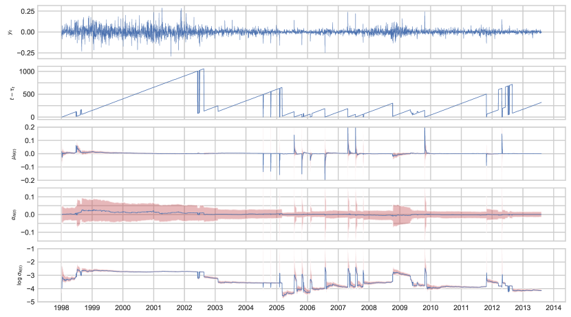
Figure 1: Change-point model applied to AMZN. From top to bottom: adjusted daily closing log-returns; number of trading days since MAP most recent change-point; posterior mean (blue) and 95% credible interval (red) for $\mu_{N(t)}$ conditional on MAP most recent change-point; posterior mean (blue) and 95% credible interval (red) for $\alpha_{N(t)}$ conditional on MAP most recent change-point; posterior mode (blue) and 95% credible interval (red) for $\log\sigma_{N(t)}$.

To illustrate inference about change-point times beyond the simple point estimate $\tau_{t}^{\mathrm{MAP}}\coloneqq\operatorname*{arg\,max}_{s}\pi_{t}(s)$, figure 2 shows a snapshot of the returns from April 2007 until July 2009 and the change-point distributions $\pi_{t}$ for $t$ corresponding to 28/09/2008, 23/02/2009, 05/05/2009, 16/07/2009. On 28/09/2008. i.e. just before the market crash, the change-point distribution (second plot from top) shows a small amount of evidence for a recent change, but most probability mass is associated with 24/07/2007 when the stock price surged after better-than-expected Q2 results were announced. The third plot down, showing the change-point distribution for $t$ corresponding to 23/02/2009 puts most of its mass around the September 2008 market crash. In the fourth plot, corresponding to 05/05/2009, the multiple modes in the distribution can be interpreted as competing hypotheses about the most recent change point: the September 2008 market crash is amongst them, followed by crises in December 2008 and January-March 2009. The bottom plot picks up the change to a period of lower volatility around the end of March 2009.

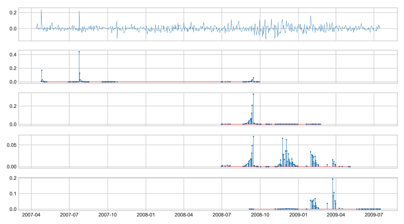
Figure 2: Change-point model applied to AMZN. Posterior distributions over time of most recent change-point, $\pi_{t}$, for $t$ corresponding to 29/09/2008, 23/02/2009, 05/05/2009, 16/07/2009. Red lines on the horizontal axes indicate range of the support of the distributions.

The top plot in figure 3 shows the returns along with the 95% credible region for each of the one-step-ahead posterior predictive distributions $p(y_{t+1}|\tau_{t+1}=\tau_{t}^{\mathrm{MAP}},y_{\tau_{t}^{\mathrm{MAP}}:t})$, i.e. (3) with $\tau_{t}^{\mathrm{MAP}}$ plugged in. The bottom plot shows these predictive credible regions pushed forward to the price.

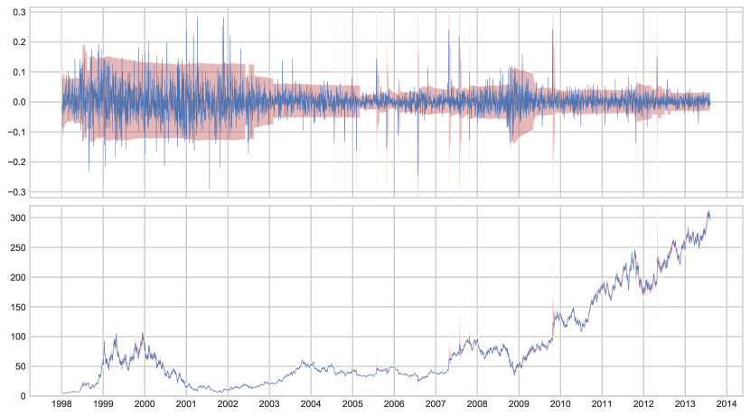
Figure 3: Change-point model applied to AMZN. Blue plot shows adjusted daily closing log-returns (top) and prices (bottom). Red shading indicates posterior predictive 95% credible interval conditional on MAP most recent change-point. See text for definition.

3.3 Hierarchical clustering

Figure 4 shows the dissimilarity matrix of Wassertein distances $W_{1}(\pi_{t}^{i},\pi_{t}^{j})$ as in (9) across the first 80 S&P 500 constituents by alphabetical order for $t$ corresponding to 16/07/2009. The reason for considering only 80 constituents is to keep the following visual results simple and easy to read. The date 16/07/2009 was chosen for purposes of illustration as it post-dates the global financial crisis and the onset of the subsequent recovery.

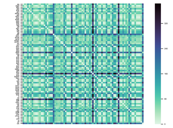
Figure 4: Dissimilarity matrix for first 80 constituents of S&P 500 for $t$ corresponding to 16/07/2009.

Whilst the dissimilarity matrix seems to show rich structure, it is not easy to directly interpret. This is where hierarchical clustering comes in: figure 3.3 shows the result of agglomerative clustering with the average linkage method, implemented in Python using the Seaborn statistical data visualization library, see https://seaborn.pydata.org and https://SciPy.org for details of the underling linkage method.

This clustering method proceeds by initializing each stock in a separate cluster, then sequentially combining nearby clusters and re-calculating between-cluster distances. The output is a dendrogram, shown on the right of figure 3.3, and a re-ordering of the rows/columns of the dissimilarity matrix to respect the structure of the dendrogram.

Once clusters of stocks are identified from this dendrogram, one may then interrogate their respective change-point distributions. To illustrate the idea, three clusters are highlighted in figure 3.3. The first cluster consists of:

• AIV, Apartment Investment and Management, a real estate investment trust;

• AFL, AFLAC Incorporated, an insurance company;

• AVB, AvalonBay Communities Real estate, an investment trust;

• AON, Aon, an insurance broker, risk, retirement and health services consulting company;

• BK, Bank of New York;

• BXP, Boston Properties, a real estate investment trust ;

• ALL, Allstate, an insurance company;

• BAC, Bank of America.

There is a clear theme of financial, real-estate and insurance sectors to this cluster. Let us examine their change-point distributions $\pi_{t}$ for $t$ corresponding to 16/07/2009: they are shown in figure 5 and the common feature is probability mass around May 2009. It was at this time that some stocks badly effected by the crisis in 2008 and early 2009 showed signs of recovery. Indeed inspecting the estimates of $\sigma_{N(t)}^{2}$ for each of these stocks (not shown) reveals there was a discrete in each of their volatilities around May 2009.

The second cluster is less sector-specific, consisting of:

• APA, Apache Corporation, a hydrocarbon exploration company;

• AZO, AutoZone, an automotive parts retailer;

• CHK, Chesapeake Energy, a hydrocarbon exploration company;

• AAPL, Apple;

• AGN, Allergan, a pharmaceutical company;

• CL, Colgate-Palmolive, a consumer products company.

Inspecting figure 3.3, it is clear that this cluster is one component of a larger cluster of 30+ stocks which have similar change-point distributions. Figure 6 indicates the feature they have in common is evidence of a volatility change, or several volatility changes, in December 2008, but little evidence of a change-point between then and June 2009. Broadly speaking, these stocks were hit by the crisis in around October 2008, but their volatility subsequently decreased sooner than the stocks in the first cluster, around the end of 2008.

The third cluster is smaller, consisting of the three stocks:

• ABT, Abbott Laboratories, a healthcare company;

• AXP, American Express;

• CAT, Caterpillar, a construction equipment manufacturer.

Figure 7 reveals that the feature these three stocks have in common is evidence of a change-point around September 2008, about the time of the market crash, but little evidence of a change-point between then and June 2009. In fact inspecting the estimated volatility parameters $\sigma_{N(t)}^{2}$ for these stocks (not shown) shows that all three of these stocks remained in a state of relatively high volatility from September 2008 until around July 2009.

[H] Hierarchical clustering dendrogram and re-ordered dissimilarity matrix for first 80 constituents of S&P 500 on 16/07/2009. Red highlighting of three clusters {AIV,AFL,AVB,AON,BK,BXP,ALL,BAC}, {APA,AZO,CHK,AAPL,AGN,CL}, {ABT, AXP, CAT}. The associated change-point distributions are shown in figures 5-7

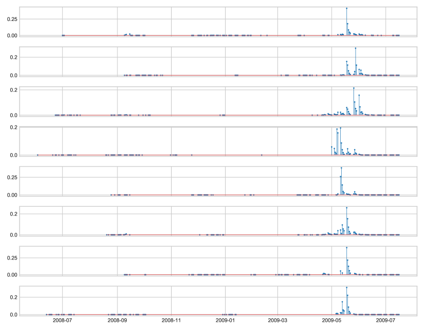
Figure 5: Posterior distributions of time of most recent change-point as of 16/07/2009 for a cluster of S&P500 constituents extracted from the dendrogram in figure 3.3, from top to bottom: AIV, AFL, AVB, AON, BK, BXP, ALL, BAC.

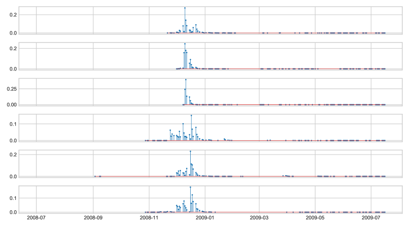
Figure 6: Posterior distributions of time of most recent change-point as of 16/07/2009 for a cluster of S&P500 constituents extracted from the dendrogram in figure 3.3, from top to bottom: APA, AZO, CHK, AAPL, AGN, CL.

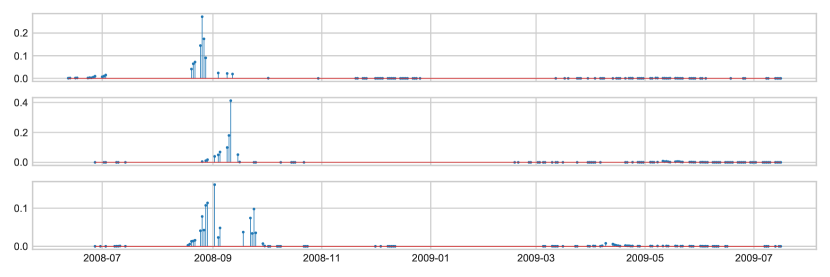
Figure 7: Posterior distributions of time of most recent change-point as of 16/07/2009 for a cluster of S&P500 constituents extracted from the dendrogram in figure 3.3, from top to bottom: ABT, AXP, CAT.

4 Extensions

There are a number of avenues open for further investigation.

In terms of the modelling of individual time series, there are number of ways the model from section 2.4 could be extended. As it stands, it doesn’t explicitly model leverage effects - that increases in volatility tend to be larger when recent returns have been negative. A number of variants of the basic GARCH model, such as Threshold-GARCH and Exponential-GARCH do model leverage effects, but involve parameters for which conjugate priors are available. It might be useful to find a half way point between such models and that of section 2.4, to achieve more accurate modelling, whilst retaining the analytic tractability which allows parameters to be integrated out.

It could be desirable to develop a more principled approach to calibrating the hyper-parameters $a,b$, $\delta_{0},\delta_{1}$, and the parameters of the prior on the inter-change-point times. This could be approached, for example, as a maximum likelihood or Bayesian inference problem. Particle Markov Chain Monte Carlo methods for the latter are given in (Whiteley et al., 2009).

It could also be interesting to explore alternative probability metrics and alternative clustering methods, for instance $k$-means using Wasserstein Barycenters (Ye et al., 2017).

References

- Adams and MacKay [2007] Ryan Prescott Adams and David J.C. MacKay. Bayesian online changepoint detection. arXiv preprint arXiv:0710.3742, 2007.
- Alonso et al. [2006] Andrés M. Alonso, José Ramón Berrendero, Adolfo Hernández, and Ana Justel. Time series clustering based on forecast densities. Computational Statistics & Data Analysis, 51(2):762–776, 2006.
- Andersen et al. [2009] Torben Gustav Andersen, Richard A. Davis, Jens-Peter Kreiß, and Thomas V. Mikosch. Handbook of financial time series. Springer Science & Business Media, 2009.
- Banerjee et al. [2005] Arindam Banerjee, Srujana Merugu, Inderjit S Dhillon, and Joydeep Ghosh. Clustering with bregman divergences. Journal of Machine Learning Research, 6(Oct):1705–1749, 2005.
- Berndt and Clifford [1994] Donald J. Berndt and James Clifford. Using dynamic time warping to find patterns in time series. In Proceedings of the 3rd International Conference on Knowledge Discovery and Data Mining, volume 10, pages 359–370. Seattle, WA, 1994.
- Bobkov and Ledoux [2016] Sergey Bobkov and Michel Ledoux. One-dimensional empirical measures, order statistics and kantorovich transport distances. preprint, 2016.
- Bollerslev [1986] Tim Bollerslev. Generalized autoregressive conditional heteroskedasticity. Journal of Econometrics, 31(3):307–327, 1986.
- Bollerslev [1987] Tim Bollerslev. A conditionally heteroskedastic time series model for speculative prices and rates of return. Review of economics and statistics, 69(3):542–547, 1987.
- Chopin [2007] Nicolas Chopin. Dynamic detection of change points in long time series. Annals of the Institute of Statistical Mathematics, 59(2):349–366, 2007.
- Corduas and Piccolo [2008] Marcella Corduas and Domenico Piccolo. Time series clustering and classification by the autoregressive metric. Computational statistics & data analysis, 52(4):1860–1872, 2008.
- Fearnhead and Liu [2007] Paul Fearnhead and Zhen Liu. On-line inference for multiple changepoint problems. Journal of the Royal Statistical Society: Series B (Statistical Methodology), 69(4):589–605, 2007.
- Lloyd [1982] Stuart Lloyd. Least squares quantization in PCM. IEEE transactions on information theory, 28(2):129–137, 1982.
- MacQueen [1967] James MacQueen. Some methods for classification and analysis of multivariate observations. In Proceedings of the fifth Berkeley symposium on mathematical statistics and probability, volume 1, pages 281–297. Oakland, CA, USA, 1967.
- Mantegna [1999] Rosario N. Mantegna. Hierarchical structure in financial markets. The European Physical Journal B-Condensed Matter and Complex Systems, 11(1):193–197, 1999.
- Marti et al. [2016] Gautier Marti, Sébastien Andler, Frank Nielsen, and Philippe Donnat. Clustering financial time series: how long is enough? In Proceedings of the Twenty-Fifth International Joint Conference on Artificial Intelligence, pages 2583–2589. AAAI Press, 2016.
- Marti et al. [2017] Gautier Marti, Frank Nielsen, Mikołaj Bińkowski, and Philippe Donnat. A review of two decades of correlations, hierarchies, networks and clustering in financial markets. arXiv preprint arXiv:1703.00485, 2017.
- Montero et al. [2014] Pablo Montero, José A Vilar, et al. Tsclust: An R package for time series clustering. Journal of Statistical Software, 62(1):1–43, 2014.
- Murphy [2012] Kevin P. Murphy. Machine learning: a probabilistic perspective. MIT press, 2012.
- Ni et al. [2018] Yang Ni, Peter Müller, Maurice Diesendruck, Sinead Williamson, Yitan Zhu, and Yuan Ji. Scalable bayesian nonparametric clustering and classification. arXiv preprint arXiv:1806.02670, 2018.
- Otranto [2008] Edoardo Otranto. Clustering heteroskedastic time series by model-based procedures. Computational Statistics & Data Analysis, 52(10):4685–4698, 2008.
- Otranto [2010] Edoardo Otranto. Identifying financial time series with similar dynamic conditional correlation. Computational Statistics & Data Analysis, 54(1):1–15, 2010.
- Peyré and Cuturi [2019] Gabriel Peyré and Marco Cuturi. Computational optimal transport. Foundations and Trends in Machine Learning, 11(5-6):355–607, 2019.
- Vilar et al. [2010] José Antonio Vilar, Andrés M Alonso, and Juan Manuel Vilar. Non-linear time series clustering based on non-parametric forecast densities. Computational Statistics & Data Analysis, 54(11):2850–2865, 2010.
- Whiteley et al. [2009] Nick Whiteley, Christophe Andrieu, and Arnaud Doucet. Bayesian computational methods for inference in multiple change-points problems. Technical report, University of Bristol, School of Mathematics, 2009. URL sites.google.com/view/nickwhiteley/.
- Ye et al. [2017] Jianbo Ye, Panruo Wu, James Z Wang, and Jia Li. Fast discrete distribution clustering using wasserstein barycenter with sparse support. IEEE Transactions on Signal Processing, 65(9):2317–2332, 2017.