The Quantum DELL System

Abstract.

We propose quantum Hamiltonians of the double elliptic many-body integrable system (DELL) and study its spectrum. These Hamiltonians are certain elliptic functions of coordinates and momenta. Our results provide quantization of the classical DELL system which was previously found in the string theory literature. The eigenfunctions for the $N$-body model are instanton partition functions of 6d $SU(N)$ gauge theory with adjoint matter compactified on a torus with a codimension two defect. As a byproduct we discover new family of symmetric orthogonal polynomials which provide an elliptic generalization to Macdonald polynomials.

1. Introduction and Main Results

Integrable many-body systems are deeply interconnected with other branches of modern mathematical physics – representation theory, algebraic geometry, string and gauge theory. We shall be discussing complex algebraic integrable systems with $N$ degrees of freedom, with a phase space being a Lagrangian fibration of complex dimension $2N$, equipped with a holomorphic symplectic 2-form, over a smooth base whose fibers are Abelian varieties. In proper Darboux coordinates $(\textbf{p},\textbf{q})=(p_{1},\dots,p_{N};q_{1},\dots,q_{N})$ the symplectic form reads $\Omega=\sum_{i}dp_{i}\wedge dq_{i}$ and there are $N$ Poisson commuting Hamiltonians $H_{1}(\textbf{p},\textbf{q}),\dots,H_{N}(\textbf{p},\textbf{q})$. One can study Hamiltonians in action-angle variables so that they only depend on action variables. In these variables the Hamiltonian evolution is linearized on the fibers which serve as the level sets of the Hamiltonians.

Since the discovery of the Seiberg-Witten solution of $\mathcal{N}=2$ supersymmetric gauge theories [Seiberg:1994aj, Seiberg:1994rs] and integrable systems related to them [Gorsky:1995zq] there has been a significant progress in understanding of integrable models and their dualities. The integrable system arises in the infrared description of the above mentioned gauge theories, which are governed by a holomorphic prepotential $\mathcal{F}(\textbf{a})$, where $\textbf{a}=(a_{1},\dots a_{N})$ are the vacuum expectation values of vector multiplets of the supersymmetric theory whose gauge group has rank $N$. The $N$-dimensional Abelian variety parameterized by the period matrix $\tau_{ij}=\partial\mathcal{F}/\partial a_{i}\partial a_{j}$ is fibered over the Coulomb branch of the theory with coordinates a.

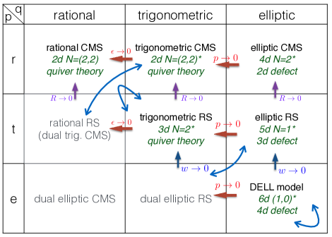
Figure 1. The ITEP Table [Mironov:2000if] of integrable many-body systems according to their periodicity properties in coordinates $q$ (columns) and momenta $p$ (rows) together with their gauge theory realizations.

The Abelian nature of the Lagrangian fibers in the algebraic description of the integrable system suggests that each coordinate and momentum can take values in complex line $\mathbb{C}$, in a complex line without origin $\mathbb{C}^{\times}$, or in an elliptic curve $\mathcal{E}=\mathbb{C}^{\times}/q^{\mathbb{Z}}$, where $q$ is a complex parameter. Therefore all many-body integrable models can be classified into rational, trigonometric and elliptic depending on where its coordinates and momenta take their values. This is summarized in Fig. 1. The first row of the table contains Calogero-Moser-Sutherland (CMS) family, the second row describes Ruijsenaars-Schneider (RS) family, whereas the last row contains models that are bispectrally dual to elliptic CMS, elliptic RS, and, finally, the DELL system. Blue double arrows describe bispectral dualities ($p-q$ dualities or Fourier transforms) between the corresponding models. Color arrows ($w\to 0,R\to 0$, etc.) show the limiting cases when the corresponding model degenerates into a simpler model.

An explicit example of such integrable system was discussed in [Gorsky:1995zq, Martinec:1995by, Donagi:1995cf]. In particular, the $\mathcal{N}=2^{*}$ theory with gauge group $U(N)$ gives rise to $N$-body elliptic Calogero-Moser model whose coupling constant is related to the mass of adjoint hypermultiplet. In this case the Liouville tori of algebraic integrable systems can be found inside the Jacobians of an algebraic curve, in other words, we are dealing with the Hitchin system [hitchin1987]. According to [Donagi:1995cf], a point in such integrable system is a holomorphic vector bundle together with and adjoint-valued one form on a genus one Riemann surface $\Sigma$. One can construct a spectral curve inside the cotangent bundle to this Riemann surface $\text{det}(u-\phi)=0$, where $u$ lives in the canonical bundle of the curve $u\in K_{\Sigma}$. The spectral curve gives rise to Hamiltonians of the integrable system depicted in the top-right corner of the table in Fig. 1.

1.1. String/Gauge Theory Background

String theory provides us with a toolkit to explore the dualities between gauge theories in various dimensions and between integrable systems which are dual to these gauge theories. In particular, there is a duality between 5d $\mathcal{N}=1^{*}$ theories and 6d theories with fundamental matter [Hollowood:2003cv]. Toric diagrams in the geometric description of those theories can be obtained one from another by a 90-degree rotation. Both models may be considered as limiting cases of the 6d theory with adjoint matter compactified on a torus with $(1,0)^{*}$ supersymmetry, see Fig. 2.

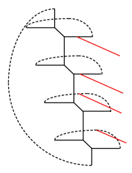
Figure 2. Toric diagram for 6d $(1,0)^{*}$ $U(4)$ theory in the presence of codimension two defect (red branes). The NS5 branes is stretched vertically, the D5 branes are stretched horizontally.

Let us consider little string theory (LST) (see [WittenLST, Losev:1998, Seiberg:1997] and [Aharony:2000] for review) on the NS5 brane within Type IIA construction with compact direction of radius $R$. Let $\phi$ be the dilaton expectation value. We can apply T-duality along the compact direction. After the T-duality we obtain the NS5 brane in Type IIB theory compactified on a circle of radius

(1.1) $$R^{\prime}=\alpha^{\prime}\frac{e^{-\phi}}{R}\,.$$

Now we can apply S-duality in Type IIB theory – the NS5 brane will turn into D5 brane and the dilaton will change its value to $\phi^{\prime}=-\phi$. Since we are dealing with the D5 brane now we can identify the field theory which lives on it – the $U(1)$ 6d $(1,1)$ theory on $\mathbb{R}^{4}\times S^{1}_{R^{\prime}}\times S^{1}_{R^{\prime\prime}}$, where $S^{1}_{R^{\prime\prime}}$ is an additional spectator compact direction on the D5 brane which was present on all branes from the beginning. This 6d theory has the following coupling constant

(1.2) $$\frac{1}{g^{2}_{\text{6d}}}=\frac{e^{-\phi^{\prime}}}{\alpha^{\prime}}=\frac{e^{\phi}}{\alpha^{\prime}}\,.$$

When the dilaton VEV is sent to infinity the theory becomes weakly coupled. Equivalently we can view this 6d theory as a 5d $\mathcal{N}=2$ theory on $\mathbb{R}^{4}\times S^{1}_{R^{\prime\prime}}$ with coupling

(1.3) $$\frac{1}{g^{2}_{\text{5d}}}=R^{\prime}\frac{1}{g^{2}_{\text{6d}}}=\alpha^{\prime}\frac{e^{-\phi}}{R}\frac{e^{\phi}}{\alpha^{\prime}}=\frac{1}{R}\,.$$

Note the the 5d coupling constant depends only on the compactification radius.

The above construction of p-q webs with D5 and NS5 branes can now be generalized to engineer more complex (quiver) 6d $(1,1)$ theories. In addition, as it has been done so in lower dimensions, we shall introduce mass of adjoint hypermultiplets, therefore deforming $(1,1)$ supersymmetry in 6d to $(1,0)^{*}$ and $\mathcal{N}=2$ supersymmetry in 5d to $\mathcal{N}=1^{*}$.

1.1.1. $Bispectral/T$-Duality

One starts with a 6d $(1,0)^{*}$ theory represented by a p-q web as in Fig. 2. Let us call this theory A. By rotating the brane web by 90 degrees we arrive to a (generically) different theory, with Neve-Schwarz and Dirichlet directions of its brane web interchanged. Let’s call it theory B. Recall that this 90 degree rotation is described by T-duality with respect to the compact circle inside the worldvolume of the NS branes. In addition to that in each p-q web Dirichlet fivebranes are also compact and the radius of the corresponding circle is $R$. Thus the T-duality merely exchanges $R$ and $R^{\prime}$. This corresponds to Fourier-Mukai transform at the level of the integrable system which is depicted by diagonal arrows in Fig. 1).

Let us look at a simple example. Consider rank two little string theory corresponding, by means of the argument we have just presented, to $\widehat{A}_{1}$ 6d $(1,0)^{*}$ theory. In this case theory A is 5d $\mathcal{N}=1^{*}$ $U(2)$ gauge theory on $\mathbb{R}^{4}\times S^{1}$, while theory B is the 6d affine quiver gauge theory with two $U(1)$ gauge groups connected to each other (see Fig. 3).

Figure 3. A Pair of dual 6d theories (bottom) and their brane realizations (top).

Note that in circular quivers an overall $U(1)$ factor inside the gauge group of the whole theory decouples and can be gauged away. This factor can be identified with one of the $U(1)$ groups in this example. The remaining $U(1)$ gauge group has two fundamental hypermultiplets which are rotated by global $SU(2)$ symmetry. In other words, theory B is nothing but $U(1)$ 6d theory with two flavors as shown in Fig. 3

Figure 4. Decoupling the $U(1)$ gauge factor in theory B from Fig 3.

Note that if the ranks of the individual gauge groups of theory B above at each node are higher the quiver remains affine. This will happen when theory A will be a quiver gauge theory with several nodes. The weakly coupled regime of the above theories can be accessed by sending $R^{\prime}\to 0$ keeping $R$ fixed, or equivalently, we can send the dilaton VEV to infinity.

1.2. Classical DELL System

In this paper we shall discuss canonical quantization of the DELL model which was studied in [Braden:1999aj, Mironov:1999vj, Braden:2001yc, Hollowood:2003cv]. As it was pointed out in [Hollowood:2003cv] term ‘double elliptic’ is a misnomer, as its momenta and coordinates as complex two-vectors lie in a 4-torus. Nevertheless, by tradition and for brevity, we shall refer to this model as DELL thereby emphasizing its double periodic nature. More recently DELL systems were studied from the point of view of modular transformations [Aminov:2013asa, Aminov:2014wra, Aminov:2017dud].

In [Braden:2003gv, Hollowood:2003cv] it was shown how to construct a spectral curve (equivalently, Seiberg-Witten curve of the 6d theory on $\mathbb{R}^{4}\times T^{2}$) of the $N$-body DELL model using the approach of matrix models and M-theory. The description involves line bundles over polarized abelian variety whose sections are generalized (higher genus) theta-functions. The resulting Seiberg-Witten curve has genus $N$, as can be seen from the toric diagram in Fig. 2, and can be holomorphically embedded into a slanted 4-torus. The Seiberg-Witten (DELL spectral) curve can be represented in the following explicit form (see [Braden:2003gv] for the detailed description)

(1.4) $$\sum_{n=0}^{\infty}m^{n}\left[\partial_{\xi}^{n}\theta(e^{\xi}|p)\right]\cdot\left[\partial_{\zeta}^{n}H(\zeta,w,\textbf{a})\right]=0\,,$$

where

(1.5) $$H(\zeta,w,\textbf{a})=\prod_{i=1}^{N}\theta\left(e^{\zeta}/a_{i}|w\right)\,,$$

$m=\log t$ is the mass of the adjoint hypermultiplet and $\theta$ is the first theta function, see (3.3). The holomorphic differentials read

(1.6) $$d\xi=\omega_{N+1}\,,\qquad d\zeta=\sum_{i=1}^{N}\omega_{i}\,,$$

so that the integrals in the homology basis of the curve $\left\{A_{1},\dots A_{N};B_{1},\dots B_{N}\right\}$ are

(1.7) $$\oint\limits_{A_{i}}\omega_{j}=\delta_{ij}\,,\qquad\oint\limits_{B_{i}}\omega_{j}=\Pi_{ij}\,,$$

where $\Pi_{ij}$ are matrix elements of a certain period matrix which obey $\sum_{j=1}^{N}\Pi_{ij}=\tau_{\text{YM}}$. The coordinates on the phase space of the integrable system are then given by the Abel map

(1.8) $$x_{i}=\sum_{j=1}^{N-1}\int\limits_{P_{0}}^{P_{j}}\omega_{i}\,,$$

for $N-1$ marked points $P_{1},\dots P_{N-1}$ of the reduced Jacobian $\mathcal{J}_{0}(\Sigma)$.

1.3. Quantization

As it was first shown in [Bullimore:2015fr] and later proven by Nekrasov (in the case of the four-dimensional $U(2)$ theory) [Nekrasov:2009rc, Alday:2010vg, Nekrasov:2013xda, Nekrasov:2015wsu, Nekrasov:2017gzb] how to find a formal spectrum of quantum elliptic integrable systems of Calogero or Ruijsenaars type. The eigenfunctions of the corresponding Hamiltonians were shown to be supersymmetric partition functions in the presence of monodromy-type defects of the Gauge/Bethe dual 4d and 5d theories with adjoint matter respectively. The eigenfunctions were represented by vacuum expectation values of local chiral observables (in 4d) and Wilson lines (in 5d):

(1.9) $$H_{i}\mathcal{Z}(p,\textbf{x})=E_{i}(p,\textbf{a})\mathcal{Z}(p,\textbf{x})\,,$$

where both $\mathcal{Z}(p,\textbf{x})$ and $E_{i}(p,\textbf{a})$ are series expansions in the instanton counting parameter $p$. As was argued in [Alday:2009fs] and used later in [Gaiotto:2013sma] the positions of a surface operator in the $U(N)$ $\mathcal{N}=2$ gauge theory are given by integrals over open paths of the corresponding Kähler classes $\omega_{i}$ (1.8). This observation explains why insertions of defect operators should be treated as the coordinates of the (complexified) integrable systems and the wavefunction $\mathcal{Z}(p,\textbf{x})$.

Mathematically the eigenfunctions of the above Hamiltonians are equivariant integrals of certain characteristic classes over the affine Laumon spaces. Negut in [Negut_2009] has proven that (1.9) holds for the elliptic Calogero-Moser Hamiltonians, in [Koroteev:2018isw] a conjecture was made stating that the K-theoretic equivariant Euler characteristic of the affine Laumon space is the eigenfunction of the elliptic Ruijsenaars-Schneider model.

1.4. Main Results

We propose the new quantum integrable system, called DELL, which for $N-1$ degrees of freedom is described by Hamiltonians

(1.10) $$\mathcal{\widehat{H}}_{a}=\widehat{\mathcal{O}}_{0}^{-1}\widehat{\mathcal{O}}_{a}\,,\qquad a=1,\ldots,N-1\,,$$

where operators $\mathcal{O}_{0},\mathcal{O}_{1},\dots,\mathcal{O}_{N-1}$ are Fourier modes of the following current

(1.11) $$\widehat{\mathcal{O}}(z)\ =\ \sum\limits_{n\in{\mathbb{Z}}}\ \widehat{\mathcal{O}}_{n}\ z^{n}\ =\ \sum\limits_{n_{1},\ldots,n_{N}=-\infty}^{\infty}\ (-z)^{\sum n_{i}}\ w^{\sum\frac{n_{i}(n_{i}-1)}{2}}\ \prod\limits_{i<j}\theta\big{(}t^{n_{i}-n_{j}}\widehat{x}_{i}/\widehat{x}_{j}|p\big{)}\ \widehat{p}_{1}^{n_{1}}\ldots\widehat{p}_{N}^{n_{N}}\,.$$

Here the canonically conjugate position and momentum operators obeying canonical q-commutation relation $\widehat{x}_{i}\widehat{p}_{j}=q^{\delta_{ij}}\widehat{p}_{j}\widehat{x}_{j}$ act on functions of positions as

(1.12) $$\widehat{x}_{i}f(x_{1},\ldots,x_{N})=x_{i}f(x_{1},\ldots,x_{N}),\qquad\widehat{p}_{i}f(x_{1},\ldots,x_{N})=f(x_{1},\ldots,qx_{i},\ldots,x_{N})\,.$$

We shall now formulate three conjectures about the properties of the DELL model, which we have checked in a number of cases. We expect that these conjectures will be proven in the near future using methods of enumerative algebraic geometry and geometric representation theory.

Conjecture 1.1.

The quantum DELL Hamiltonians $\mathcal{H}_{1},\dots\mathcal{H}_{N-1}$ in (1.10) commute,

(1.13) $$[\mathcal{\widehat{H}}_{a},\mathcal{\widehat{H}}_{b}]=0\,,\qquad a\neq b\,.$$

We were able to check the commutativity of DELL Hamiltonians up to several orders ($w^{2},p^{2}$ for $N=2,3$ and $w^{2},p^{1}$ for $N=4$) in expansion in elliptic parameters $p$ and $w$, which gives us confidence that the conjecture should hold. As the reader can see the DELL Hamiltonians are highly non-local as they involve formal infinite series of functions of shift operators, which severely limits the computational ability to verify the conjecture. We expect that the general proof to be found some time in the near future.

The DELL Hamiltonians provide a two-parameter $(w,p)$ generalization of the trigonometric Ruijsenaars-Schneider integrable system, whose eigenfunctions are also known as Macdonald polynomials. The common eigenfunctions of the full DELL Hamiltonians are therefore a natural candidate to replace the Macdonald polynomials in the double-elliptic setting, and we will call them double elliptic Macdonald functions. They depend on four parameters – $q,t$ and $p,w$. We expect them to agree with ‘affine Macdonald polynomials’ in representation theory [Etingof:ab], similar in the number of parameters and limiting behavior.

We have also found the formal spectrum of DELL Hamiltonians which can be formulated using defect partition functions of a 6d gauge theory on $\mathbb{R}^{4}\times T^{2}$ and is similar to the analogous 5d version, albeit with an important difference.

Conjecture 1.2.

Let $\textbf{x}=(x_{1},\dots,x_{N})$ be the position vector, $\mathscr{Z}(p,\textbf{x})$ be a properly normalized equivariant elliptic genus of the affine Laumon space in the limit $\epsilon_{2}\to 0$. Then there exists a function $\lambda(z,\textbf{a},w,p)$ such that

(1.14) $$\widehat{\mathcal{O}}(z)\mathscr{Z}(p,\textbf{x})=\lambda(z,\textbf{a},w,p)\ \widehat{\mathcal{O}}_{0}\mathscr{Z}(p,\textbf{x})\,.$$

In particular, by expanding currents $\widehat{\mathcal{O}}(z)$ as in (1.11) and $\lambda(z,\textbf{a},w,p)=\sum_{n}\lambda_{n}(\textbf{a},w,p)z^{n}$ in $z$ we obtain similar relations for each operator $\widehat{\mathcal{O}}_{n}$, or, using (1.10) we obtain the eigenvalue problem for DELL Hamiltonians

(1.15) $$\widehat{\mathcal{H}}_{n}\mathcal{Z}^{6d/4d}_{\text{inst}}(w,p,\textbf{x})=\lambda_{n}(\textbf{a},w,p)\mathcal{Z}^{6d/4d}_{\text{inst}}(w,p,\textbf{x})\,.$$

At the moment we know the eigenvalues $\lambda_{n}(\textbf{a},w,p)$ in terms of first several terms in series expansion in $w$ and $p$. In the limiting cases, when either $w$ or $p$ vanish (and we land onto the eRS model or on the dual RS model) we have complete control of these functions and know of their interpretations in terms of the corresponding gauge theories. Yet, at the moment we are lacking a complete understanding of a geometric or physical (in terms of a vacuum expectation value of some BPS observable in the 6d theory) meaning of $\lambda_{n}(\textbf{a},w,p)$. We shall however make an educated guess about these matters in Sec. 4.4. We hope to understand it in the nearest future.

However, in the limit of $w\to 0$ in which the DELL model becomes the eRS model, we conjecture the following result, inspired by study of Chern-Simons theory on $S^{3}$, which compliments the result of [Bullimore:2015fr]:

Conjecture 1.3.

Let $\textbf{x}=(x_{1},\dots x_{N})$ be the position vector of the eRS model and $\mathcal{Z}^{{\text{RS}}}(\textbf{a},\textbf{x})=\lim\limits_{w\to 0}\mathcal{Z}^{6d/4d}_{\text{inst}}(w,p,\textbf{x})$ is its wavefunction. Then the following equality holds

(1.16) $$\mathcal{H}_{i}\mathcal{Z}^{{\text{RS}}}(\textbf{a},\textbf{x})=\lambda_{i}(\textbf{a})\mathcal{Z}^{{\text{RS}}}(\textbf{a},\textbf{x})\,,\qquad i=1,\dots,N-1\,.$$

where the eigenvalues read

(1.17) $$\lambda_{i}(\textbf{a})=(-1)^{i}\frac{\theta(t^{N})}{\theta(t)}\frac{\mathcal{Z}^{{\text{RS}}}(\textbf{a},t^{\vec{\rho}}q^{\vec{\omega_{i}}})}{\mathcal{Z}^{{\text{RS}}}(\textbf{a},t^{\vec{\rho}})}\,,\qquad i=1,\dots,N-1$$

where $\vec{\omega_{i}}$ is the $i$-th fundamental weight of representation of $SU(N)$ and $\vec{\rho}=(-N/2,-(N-1)/2,\dots,(N-1)/2,N/2)$ is the $SU(N)$ Weyl vector.

This formula expresses the eigenvalue for the DELL eigenvalue problem in terms of the eigenfunction. This generalizes the well-known nonelliptic result, and may have topological implications in terms of the elliptic Chern-Simons theory, which remains to be constructed.

1.5. Connection to Aminov-Mironov-Morozov DELL Hamiltonians

There is a different approach to the DELL system in the literature which is discussed in [Mironov:1999vi] and more recently in [Aminov:2016ruk]. The explicit $N$-body Hamiltonians are written in formula (2.1) of [Aminov:2016ruk] and possess some similarity with ours, however, characteristics a and b in the definition of theta functions (2.1) are slightly different. More importantly, theta functions which we use in our paper (they are borrowed from [Braden:2003gv]) have constant period matrix (2.3), whereas the period matrix from the Aminov-Mironov-Morozov paper $T_{ij}=\partial_{i}\partial_{j}\mathcal{F}$ is the hessian of the 6d Seiberg-Witten prepotential which is known by the authors up to several orders in instanton coupling. Additionally genera of our and AMM spectral curves are different for given $N$.

It is clear this point that a significant amount of effort is needed in order to match the two constructions; nevertheless we stay optimistic in this regard given the fact that both models arise from the same gauge theory.

1.6. Future Directions

We would like to outline some directions of future research which is related to physics and mathematics around the DELL system.

• Recently, due to a significant progress in F-theory, Seiberg-Witten curves for quiver 6d theories of some simply-laced types were constructed [Haghighat:2016jjf, Haghighat:2018dwe]. One should be able to generalize our construction to these quiver theories and perform quantization of those models.

• We hope that the proofs of the conjectures which we have outlined earlier in this section will be found and connections with the representation theory of elliptic algebras (such as Sklyanin algebra, or possibly elliptic DAHA) will be established. The structure of relation (1.14) suggests a special role of operator $\widehat{\mathcal{O}}_{0}$, which needs to be understood in details. We hope that current (1.11) has both representation theoretic and string theory meanings.

• It will be interesting to study various limiting cases of the DELL Hamiltonians (1.10). In particular, the so-called Inozemtsev limit [inozemtsev1989] when $t\to\infty$ yields the reduction of the elliptic Calogero model to affine Toda model, while the elliptic RS modes becomes the affine q-Toda model. The Inozemtsev limit of the DELL model is yet to be understood. In terms of dual gauge theories the $t\to\infty$ limits corresponds to sending the mass of adjoint hypermultiplets to infinity. See [Aminov:2017dud] for some preliminary discussion on these matters.

• Recently the correspondence between integrability and $\mathcal{N}=2$ SUSY was revisited in the regime $N\to\infty$, or when the number of the degrees of freedom becomes large. In [Koroteev:2016, Koroteev:2018a] it was shown that the spectrum of the (difference) quantum intermediate long wave system (ILW) can be reproduced from the quantum spectrum of the elliptic RS model (1.9) at large $N$. Geometrically ILW energies are related to operators of quantum multiplication by quantum tautological bundles in the equivariant K-theory of the moduli space of $U(1)$ instantons. One needs to understand how the upgrade from eRS to DELL is reflected on the geometric side.

• In general, any question which was asked and answered about any model from Fig. 1 needs to be addressed for the DELL model.

1.7. Structure of the Paper

In the next Section we remind the reader about the classical Seiberg-Witten geometry of the 6d theory with adjoint matter with eight supercharges compactified on $T^{2}$. In Section 3 the quantum DELL Hamiltonians are discussed as well as their limits to the eRS and dual eRS models. Section 4 introduces instanton partition functions of the 6d theory with monodromy defects using characters of the affine Laumon space. We demonstrate that this partition function in the Nekrasov-Shatashvili limit satisfies the formal difference DELL equation. Finally, in Section 5 we discuss in more details polynomial solutions of the DELL difference equation. In particular, we address the properties of the new elliptic Macdonald functions.

1.8. Acknowledgements

This manuscript took some time to complete primarily due to the technical computational difficulties of expressions involving double-periodic functions. We would like to thank numerous people with whom we discussed these and other matters, as well as various institutions which we visited in the last several years, but our special acknowledgements go to Babak Haghigat, Wenbin Yan, Can Kozcaz and Francesco Benini who participated in earlier stages of the project.

2. Seiberg-Witten Geometry

The construction of [Braden:2003gv, Hollowood:2003cv] uses the M-theory compactification where two distinct tori are involved – one spacial $T^{2}$, which is a part of the gauge theory worldvolume, while the other (sometimes referred to as electro-magnetic) torus, after the compactification provides the gauge theory with maxima supersymmetry. This supersymmetry is broken to a $(1,0)^{*}$ subgroup once we include an equivariant action of $\mathbb{C}^{\times}$ along the remaining flat noncompact directions whose character is equal to $t$ such that $\log t\sim m$, where $m$ is the mass of the adjoint hypermultiplet.

The Seiberg-Witten curve $\Sigma$ for 6d $(1,0)^{*}$ theory compactified on $T^{2}_{w}$ was derived in [Braden:2003gv]. The description involves line bundles over polarized abelian varieties whose sections are generalized theta-functions. Such genus-$g$ theta function with period $g\times g$-matrix $\Pi$ reads

(2.1) $$\Theta\left[\begin{array}[]{c}\textbf{a}\\ \textbf{b}\end{array}\right](\textbf{Z}|\Pi)=\sum\limits_{\textbf{m}\in\mathbb{Z}^{g}}\exp\left(\pi i(\textbf{m}+\textbf{a})\cdot\Pi\cdot(\textbf{m}+\textbf{a})+2\pi i(\textbf{Z}+\textbf{b})\cdot(\textbf{m}+\textbf{a})\right)\,,$$

where $\textbf{a},\textbf{b},\textbf{Z}$ and m are $g$-dimensional vectors.

The Seiberg-Witten curve can be written in terms of genus-$(N+1)$ theta function as follows

(2.2) $$\Theta\left[\begin{array}[]{ccc}\frac{1}{2}&\cdots&\frac{1}{2}\\ \frac{1}{2}&\cdots&\frac{1}{2}\end{array}\right]\left(z,Nm(x-a_{1})),\dots,Nm(x-a_{N})|\widehat{\Pi}\right)=0\,,$$

using the following $(N+1)\times(N+1)$ period matrix

(2.3) $$\widehat{\Pi}=\begin{pmatrix}\tau_{1}&gm&gm&\cdots&gm\\ gm&\tau_{2}&0&\cdots&0\\ gm&0&\tau_{2}&\cdots&0\\ \vdots&\vdots&\vdots&\ddots&0\\ gm&0&\cdots&0&\tau_{2}\end{pmatrix}\,,$$

where the elliptic parameters are $p=e^{\pi i\tau_{1}}$ and $w=e^{\pi i\tau_{2}}$. One can show that this form of $\Sigma$ is equivalent to (1.4).

One may think the spectral curve $\Sigma$ of the $N$-body DELL model as a 56-torus $T^{2}_{w}$ with additional $N$ handles attached to it. The corresponding $N$ B-periods depend on the mass parameter $m$. In the limit $m\to 0$ those handles detach and $\Sigma$ splits into a disjoint union of $(N+1)$ tori. As was mentioned earlier, $\Sigma$ can be expresses as infinite sum (1.4) where the limit $m\to 0$ is manifest.

The original references [Braden:2003gv, Hollowood:2003cv] discuss a different presentation of $\Sigma$ using a sum of genus-2 theta functions

(2.4) $$\sum_{j=1}^{N-1}a_{j}\Theta\left[\begin{array}[]{cc}0&\frac{j}{N}\\ 0&0\end{array}\right]\left(z\ \ \ gx\left|\begin{array}[]{cc}\tau_{1}&gm\\ gm&\tau_{2}\end{array}\right.\right)=0\,,$$

where $a_{j}$ are certain theta functions of the coordinates x. The limiting cases $p\to 0$ and $w\to 0$ when DELL model reduces to dual eRS and to the eRS models respectively are also discussed in [Braden:2003gv].

3. The Quantum DELL Integrable System

In this section we introduce quantum DELL system as a set of commuting formal difference operators in $q$. In terms of the canonically conjugate positions and momenta these difference operators act as

(3.1) $$\widehat{x}_{i}f(x_{1},\ldots,x_{N})=x_{i}f(x_{1},\ldots,x_{N}),\qquad\widehat{p}_{i}f(x_{1},\ldots,x_{N})=f(x_{1},\ldots,qx_{i},\ldots,x_{N})$$

Let $\widehat{\mathcal{O}}(z)$ be the DELL current which is a series in formal variable $z$

(3.2) $$\widehat{\mathcal{O}}(z)\ =\ \sum\limits_{n\in{\mathbb{Z}}}\ \widehat{\mathcal{O}}_{n}\ z^{n}\ =\ \sum\limits_{n_{1},\ldots,n_{N}=-\infty}^{\infty}\ (-z)^{\sum n_{i}}\ w^{\sum\frac{n_{i}(n_{i}-1)}{2}}\ \prod\limits_{i<j}\theta\left(t^{n_{i}-n_{j}}\frac{\widehat{x}_{i}}{\widehat{x}_{j}}\Big{|}p\right)\ \widehat{p}_{1}^{n_{1}}\ldots\widehat{p}_{N}^{n_{N}}\,,$$

where we use the following genus one theta function

(3.3) $$\theta(x|p)=\prod\limits_{k=0}^{\infty}(1-p^{2k+2})(1-p^{2k}x)(1-p^{2k+2}/x)=\sum\limits_{k=-\infty}^{\infty}\ (-x)^{k}\ p^{k^{2}-k}\,.$$

Its $z$-modes $\widehat{\mathcal{O}}_{n}$ are used to construct DELL Hamiltonians.

We have presented DELL Hamiltonians in the form (3.2), where the sum is taken over quadratic powers of elliptic parameter $\omega$ multiplied by theta functions involving $p$, since it is convenient for the calculations of the spectrum in the next section. Equivalently one could present (3.2) in a reciprocal form, where the roles of $w$ and $p$ are swapped.

Despite that fact that formula (3.2) provides an infinite set of operators $\widehat{\mathcal{O}}_{n}(z)$ only first $N$ of them are completely independent. We shall discuss periodicity in index $n$ momentarily.

3.1. Quasiperiodicity

It is easy to show that $\widehat{\mathcal{O}}(z)$ is quasiperiodic in $z$ with weight

(3.4) $$\widehat{\mathcal{O}}(wz)=\Big{(}(-1)^{N}z^{-N}t^{-N(N-1)}q^{-J}\Big{)}\ \widehat{\mathcal{O}}(z),\qquad J=j_{1}+\ldots+j_{N}\,,$$

and hence can be decomposed in the basis of theta functions of the appropriate level

(3.5) $$\widehat{\mathcal{O}}(z)=\sum\limits_{a=0}^{N-1}\ \widehat{\mathcal{O}}_{a}\ \theta^{(N)}_{a}(z)\,,$$

where the basis consists of the following $N$ functions

(3.6) $$\theta^{(N)}_{a}(z)=z^{a}\ \sum\limits_{n\in{\mathbb{Z}}}\ w^{Nn(n-1)/2+an}\ \big{(}(-z)^{N}t^{N(N-1)}q^{J}\big{)}^{n}\,,$$

and represents an elliptic deformation of the monomial basis $\{1,z,\ldots,z^{N-1}\}$ in the space of polynomials of degree $(N-1)$. This implies that $\widehat{\mathcal{O}}(z)$ contains as much information as the first $N$ modes (from $0$th to $(N-1)$st).

3.2. DELL Hamiltonians

We define quantum Hamiltonians of the DELL integrable system as the following $N-1$ operators

(3.7) $$\mathcal{\widehat{H}}_{a}=\widehat{\mathcal{O}}_{0}^{-1}\widehat{\mathcal{O}}_{a},\qquad\qquad a=1,\ldots,N-1\,,$$

which are manifestly nonlocal. We have checked using Mathematica that DELL Hamiltonians commute, as we stated it in Conjecture 1.13. Note that modes $\mathcal{O}_{a}$ do not commute for different $a$, only if we compose them with the inverse of $\mathcal{O}_{0}^{-1}$ as in (3.7) they will.

One can see from (3.2) and (3.7) that expression

(3.8) $$\mathcal{L}(z):=\widehat{\mathcal{O}}_{0}^{-1}\widehat{\mathcal{O}}(z)=\sum\limits_{a=0}^{\infty}z^{n}\,\widehat{\mathcal{O}}_{0}^{-1}\widehat{\mathcal{O}}_{a}=1+z\,\mathcal{\widehat{H}}_{1}+z^{2}\,\mathcal{\widehat{H}}_{2}+\dots$$

generates all DELL Hamiltonians and is the elliptic analogue of the characteristic polynomial of a Lax matrix det$(1-zL)$. Indeed, due to quasiperiodicity (3.4) only first $N$ Hamiltonians are independent. Thus $z$ plays the role of the spectral parameter.

The commutativity of DELL hamiltonians therefore can be succinctly expressed as

(3.9) $$[\mathcal{L}(z),\mathcal{L}(z^{\prime})]=0\,.$$

3.3. Example: Rank 1 System

Let us consider the DELL model which comes from the SU(2) 6d gauge theory in more details. It has been previously understood in [Braden:1999aj, Mironov:1999vj].

The genus-2 Riemann theta function with elliptic parameters $p$ and $w$ explicitly has the following form

(3.14) $$\Theta\left[\begin{array}[]{cc}a&b\\ 0&0\end{array}\right] \left({q}\ \ \ g{p}\left|\begin{array}[]{cc}\tau_{1}&gm\\ gm&\tau_{2}\end{array}\right.\right)$$

(3.15) $$=\sum\limits_{k_{1},k_{2}=-\infty}^{\infty}\ p^{(k_{1}+a)^{2}-a^{2}}\ w^{(k_{2}+b)^{2}-b^{2}}\ t^{2(k_{1}+a)(k_{2}+b)}\ \big{(}-{Q}^{2}\big{)}^{k_{1}+a}\ \big{(}{P}^{2}\big{)}^{k_{2}+b}\,,$$

where we introduced the following exponential parameters

(3.16) $$q=e^{\pi ig},\ \ \ t=e^{\pi img},\ \ \ p=e^{\pi i\tau_{1}},\ \ \ w=e^{\pi i\tau_{2}},\ \ \ {P}=e^{\pi ig{p}},\ \ \ {Q}=e^{\pi i{q}}\,.$$

Here $p$ and $w$ are the two elliptic parameters. Note, that the contribution $p^{-a^{2}}w^{-b^{2}}$ normalizes the theta function so that it is a series in positive integer powers of $p,w$.

Using (3.15) we can show that for $N=2$ the only DELL Hamiltonian can be written in terms of genus-2 theta functions

(3.17) $$\mathcal{\widehat{H}}=\widehat{\mathcal{O}}_{0}^{-1}\widehat{\mathcal{O}}_{1}\,,$$

where

(3.18) $$\widehat{\mathcal{O}}_{0}=\Theta\left[\begin{array}[]{cc}\frac{1}{2}&0\\ 0&0\end{array}\right]\left(\frac{\widehat{x}_{2}}{\widehat{x}_{1}},\frac{\widehat{p_{2}}}{\widehat{p_{1}}}\right)\,,\qquad\widehat{\mathcal{O}}_{1}=\Theta\left[\begin{array}[]{cc}\frac{1}{2}&\frac{1}{2}\\ 0&0\end{array}\right]\left(\frac{\widehat{x}_{2}}{\widehat{x}_{1}},\frac{\widehat{p_{2}}}{\widehat{p_{1}}}\right)\,.$$

The above formulae provide a closed form for the Hamiltonian in terms of higher genera theta functions; it is unclear if a generalization exists for DELL models with $N>2$.

In the limit $w\to 0$ for $N=2$ we get from (3.2)

(3.19) $$\mathcal{O}(z)=\theta\left(\frac{x_{1}}{x_{2}}\Big{|}p\right)-z\left(\theta\left(\frac{tx_{1}}{x_{2}}\Big{|}p\right)p_{1}+\theta\left(\frac{x_{1}}{tx_{2}}\Big{|}p\right)p_{2}\right)+z^{2}\theta\left(\frac{x_{1}}{x_{2}}\Big{|}p\right)p_{1}p_{2}\,,$$

which yields the integrals of motion of the two-body eRS model

(3.20) $$\mathcal{H}_{1}=\frac{\mathcal{O}_{1}}{\mathcal{O}_{0}}=\frac{\theta\left(t\frac{x_{1}}{x_{2}}\Big{|}p\right)}{\theta\left(\frac{x_{1}}{x_{2}}\Big{|}p\right)}p_{1}+\frac{\theta\left(t\frac{x_{2}}{x_{1}}\Big{|}p\right)}{\theta\left(\frac{x_{2}}{x_{1}}\Big{|}p\right)}p_{2}\,,\qquad\mathcal{H}_{2}=\frac{\mathcal{O}_{2}}{\mathcal{O}_{0}}=p_{1}p_{2}\,.$$

In the limit $p\to 0$ we get from (3.3) $\theta(z|0)=1-z$ and (3.2) reads

$$\mathcal{O}(z) =\sum_{n_{1}\in\mathbb{Z}}w^{n_{1}^{2}}\left(1-t^{2n_{1}}\frac{x_{1}}{x_{2}}\right)\left(\frac{p_{1}}{p_{2}}\right)^{n_{1}}$$

$$-z\sum_{n_{1}\in\mathbb{Z}}w^{n_{1}^{2}-n_{1}}\left(\left(1-t^{2n_{1}-1}\frac{x_{1}}{x_{2}}\right)\left(\frac{p_{1}}{p_{2}}\right)^{n_{1}}p_{2}+\left(1-t^{-2n_{1}+1}\frac{x_{2}}{x_{1}}\right)\left(\frac{p_{2}}{p_{1}}\right)^{n_{1}}p_{1}\right)$$

(3.21) $$+z^{2}\sum_{n_{1}\in\mathbb{Z}}w^{n_{1}^{2}}\left(1-t^{2n_{1}}\frac{x_{1}}{x_{2}}\right)\left(\frac{p_{1}}{p_{2}}\right)^{n_{1}}p_{1}p_{2}+\dots\,,$$

and can be summed as follows

(3.22) $$\mathcal{O}(z)\ =\ \theta(zp_{1}|w)\theta(zp_{2}|w)-\frac{x_{1}}{x_{2}}\ \theta(ztp_{1}|w)\theta\left(\frac{z}{t}p_{2}|w\right)\,.$$

This yields a twisted version of the dual eRS Hamiltonians after expanding in modes

$$\mathcal{O}_{0}=\theta(-p_{1}/p_{2}|w)-x_{1}/x_{2}\ \theta(-t^{2}p_{1}/p_{2}|w),\ \ \$$

(3.23) $$\mathcal{O}_{1}=\theta(-wp_{1}/p_{2}|w)-tx_{1}/x_{2}p_{1}\ \theta(-wt^{2}p_{1}/p_{2}|w)\,,$$

and the other modes can be obtained by periodicity.

3.4. Quiver Generalization. Spin-DELL

The above construction suggests a straightforward generalization to $\widehat{A}$-type 6d quiver gauge theories. Given an affine quiver theory of $L$ $U(N)$ gauge groups we propose the following generating function

$$\widehat{\mathcal{O^{S}}}(z)\ =\ \sum\limits_{n\in{\mathbb{Z}}}\ \widehat{\mathcal{O^{S}}}_{n}\ z^{n}$$

(3.24) $$=\sum\limits_{a=1}^{L}\sum\limits_{\textbf{n}_{a}\in\mathbb{Z}^{N}}\ (-z)^{\sum n_{a,i}}\ w^{\sum\frac{n_{a,i}(n_{a,i}-1)}{2}}\ \prod\limits_{a=1}^{L}\prod\limits_{i<j}\theta\left(t^{n_{a,i}-n_{a,j}}\frac{\widehat{x}_{a,i}}{\widehat{x}_{a,j}}\Big{|}p\right)\ \widehat{p}_{a,1}^{n_{a,1}}\ldots\widehat{p}_{a,N}^{n_{a,N}}\,,$$

where subscript $a$ enumerates gauge groups in the quiver, $\textbf{n}_{a}=\{n_{a,1},\dots,n_{a,N}\}$, and the mode number is $n=\sum_{a,i}n_{a,i}$. We can call this model spin-DELL analogously to the spin-Calogero system. In the brane construction coordinates $x_{a,i}$ show the position of endpoints of Lagrangian branes corresponding to $a$th gauge group.

4. Defect Partition Function and Spectrum

Our task is to compute instanton partition functions of 6d $(1,0)^{*}$ theories with monodromy defects and relate them to the eigenfunctions of elliptic integrable systems. In [Bullimore:2015fr] it was shown how to do this computation for 5d $\mathcal{N}=1^{*}$ theory. The 6d $(1,0)^{*}$ theories are natural generalizations of the corresponding 5d $\mathcal{N}=1^{*}$ theories. In particular, the 6d theories with the same matter content as their 5d cousins are anomaly free.

4.1. Instanton Partition Function

Let us briefly review the essential ingredients of the instanton calculus [Nekrasov:2002qd, Nekrasov:2003rj] with ramification [Alday:2010vg, Nawata:2014nca, Bullimore:2015fr, Nekrasov:2017rqy]. What follows represents a short summary of Section 4 of [Bullimore:2015fr] albeit modified for the 6d theories on $\mathbb{R}^{4}\times T^{2}$ from the 5d theories on $\mathbb{R}^{4}\times S^{1}$.

The ADHM construction of the moduli space of $k$ $U(N)$ instantons $\mathcal{M}_{k,N}$ is a hyperkahler quotient which can be conveniently represented as an $\widehat{A}_{0}$ quiver variety with framing $W=\mathbb{C}^{N}$ as well as $A,B\in\text{Hom}(V,V),\,I\in\text{Hom}(V,W),\,J\in\text{Hom}(W,V)$. Here $V=\mathbb{C}^{k}$. $U(k)$ naturally acts on these matrices. Then the moduli space $\mathcal{M}_{k,N}$ is given by the holomorphic symplectic quotient $\mu^{-1}(0)//_{\theta}GL(k,\mathbb{C})$ of the zero locus of the complex moment map $\mu=[A,B]+IJ$ over the complexified group action in the presence of certain stability conditions.

Let $T=\mathbb{C}^{\times}_{q_{1}}\times\mathbb{C}^{\times}_{q_{2}}\times\mathbb{T}(GL(k;\mathbb{C}))$ be the maximal torus of the action of the global symmetry on $\mathbb{R}^{4}\times\mathcal{M}_{k,N}$. Here $\mathbb{R}^{4}$ is the spacetime where the 4d gauge theory lives. Fixed points of this action are parameterized by Young tableaux $\lambda_{i},\,i=1,\dots,N$ for each $U(1)$ factor of the gauge group $U(N)$.

The $T$-equivariant Chern character of universal bundle over $\mathcal{M}_{k,N}$ at the fixed point labelled by tableau $\lambda$ reads

(4.1) $$\mathscr{U}=\mathscr{W}-(1-q_{1})(1-q_{2})\mathscr{V}\,,$$

where

(4.2) $$\mathscr{W}=\sum_{i=1}^{N}e^{a_{i}}\,,\qquad\mathscr{V}=\sum_{i=1}^{N}e^{a_{i}}\sum_{(i,j)\in\lambda_{i}}^{k}q_{1}^{(i-1)}q_{2}^{(j-1)}\,,$$

where $q_{1}=e^{\epsilon_{1}},q_{2}=e^{\epsilon_{2}},e^{a_{1}},\dots,e^{a_{N}}$ are the equivariant parameters of $T$. Using $\mathscr{U}$ we define the equivariant character of the tangent space to $\mathcal{M}_{k,N}$ at $\lambda$

(4.3) $$\chi_{1}=-(1-q_{1})(1-q_{2})\mathscr{V}\mathscr{V}^{*}+q_{1}q_{2}\mathscr{W}\mathscr{V}^{*}+\mathscr{W}^{*}\mathscr{V}\,,$$

where the conjugation ^∗ corresponds to inverting the equivariant parameters. Due to the presence of the adjoint matter with mass $m$ we need to multiply the above expression by

(4.4) $$\chi_{2}=(1-Q_{m}q_{1}^{-1}q_{2}^{-1})\chi_{1}\,,$$

where $Q_{m}=e^{m}$. The equivariant character can always be written as follows

(4.5) $$\chi_{2}=\sum_{\alpha}n_{\alpha}e^{\omega_{\alpha}}\,,$$

from which we compute the 6d instanton partition function. The contribution to the topological sector with $k$ instantons reads

(4.6) $$\mathcal{Z}_{k}=\frac{1}{\theta_{1}(\omega_{\alpha}|w)^{n_{\alpha}}}\,,$$

where $w$ is the modular parameter of the torus on which the 6d theory is compactified, and the sum is taken over all Young diagrams of size $k$. The full 6d partition function is obtained by summing over all topological sectors (see also [Kim:2015uq])

(4.7) $$\mathcal{Z}=\sum_{k}p^{k}\mathcal{Z}_{k}\,,$$

where $p$ is a dimensionless combination of the Yang-Mills coupling and the torus area.

4.2. Ramification

Now we need to upgrade the construction by introducing a defect [Alday:2010vg, Bullimore:2015fr]. The codimension-two defect wrapping $\mathbb{C}_{q_{1}}$ plane is described by specifying the eigenvalues of the $U(N)$ gauge field monodromy

(4.8) $$\oint A^{a}=2\pi m_{a},\qquad a=1,\dots,N\,,$$

where

(4.9) $$m^{a}=(\underbrace{m_{1},\dots,m_{1}}_{n_{1}},\underbrace{m_{2},\dots,m_{2}}_{n_{2}},\dots,\underbrace{m_{s},\dots,m_{s}}_{n_{s}})$$

In the presence of such a defect the symmetry is broken to the Levi subgroup $U(n_{1})\times\dots\times U(n_{s})$ of $U(N)$. The defect is of maximal type if $s=N$, it is of simple type if $s=1$.

The ADHM construction and hence the instanton character formula needs to be modified in order to take into account the action of the orbifold $\mathbb{Z}_{s}$ symmetry on the moduli space. Due to the orbifolding each instanton sector splits into $s$ subsectors

(4.10) $$\mathcal{M}_{k,N}\to\bigoplus\limits_{k_{1},\dots,k_{s}}\mathcal{M}_{k_{1},\dots,k_{s},N}\,,$$

such that $k_{1}+\dots+k_{s}=k$. The equivariant character of the tangent space to the moduli space of ramified instantons $T^{*}\mathcal{M}_{\rho,k_{1},\dots,k_{s}}$ reads

(4.11) $$\chi_{\rho,\boldsymbol{\lambda}}(a,\epsilon_{1},\epsilon_{2})=\frac{1}{s}\sum\limits_{r=1}^{s}\chi_{2}\left(a_{j,\alpha}-\frac{\epsilon_{2}+2\pi r}{s}j,\epsilon_{1},\frac{\epsilon_{2}+2\pi r}{s}\right)=\sum\limits_{\alpha}n_{\alpha}e^{\omega_{\alpha}}\,,$$

were $\chi_{2}$ is given in (4.4), and the partition $\rho$ has $s$ columns.

In the ramified setting fixed points are labelled by two indices $\lambda_{j,\alpha},\,j=1,\dots,s,\,\alpha=1,\dots,n_{s}$. Then the $i$-th column of $\lambda_{j,\alpha}$ contributes to the instanton sector $i+j-1$ mod $N$. We denote this sector as $k_{j}(\boldsymbol{\lambda})$. The Nekrasov partition function (4.6) takes the following form

(4.12) $$\mathcal{Z}^{6d/4d}_{\text{inst}}=\sum_{\boldsymbol{\lambda}}x_{1}^{k_{1}(\boldsymbol{\lambda})}\dots x_{s}^{k_{s}(\boldsymbol{\lambda})}\mathcal{Z}_{\rho,\boldsymbol{\lambda}}\,,$$

where

(4.13) $$\mathcal{Z}_{\rho,\boldsymbol{\lambda}}=\prod_{\alpha}(\theta(\omega_{\alpha}|w))^{-n_{\alpha}}\,,$$

and such that $x_{1}\dots x_{s}=1$.

4.3. Eigenfunctions and the Difference Equation

In order to establish and eigenvalue problem we need to take the Nekrasov-Shatashvili limit $q_{2}\to 1$ $(\epsilon_{2}\to 0)$. Since the partition function is singular in this limit we need to normalize the defect partition function as

(4.14) $$\mathscr{Z}(\textbf{x},\textbf{a},q_{1},Q_{m},p,w)=\lim\limits_{\epsilon_{2}\to 0}\left(\dfrac{\mathcal{Z}^{6d/4d}_{\text{inst}}}{\mathcal{Z}}\right)\,,$$

where $\mathcal{Z}^{6d/4d}_{\text{inst}}$ is the defect partition function (4.12) in the $\mathcal{N}=(1,0)^{*}$ 6d $U(N)$ gauge theory with a massive adjoint, and $\mathcal{Z}$ is given in (4.7).

The function $\mathscr{Z}$ satisfies the following DELL difference equation

(4.15) $$\widehat{\mathcal{O}}(z)\mathscr{Z}=\lambda(z)\ \widehat{\mathcal{O}}_{0}\mathscr{Z}\,,$$

where the eigenvalue can be expanded in $z$-modes $\lambda(z)=\sum_{r}z^{r}\lambda_{r}(\textbf{a},q_{1},Q_{m},p,w)$, where each coefficient is a double series in the elliptic parameters

(4.16) $$\lambda_{r}=\sum_{m,n}p^{m}w^{n}\lambda_{r,m,n}(q_{1},Q_{m})\,,$$

where $\lambda_{r,m,n}(q_{1},Q_{m})$ are some rational functions of its arguments (see below and in App. A). The current $\lambda(z)$ possesses the same quasi-periodicity properties as the operator $\widehat{\mathcal{O}}(z)$ (3.4).

4.4. Comments on Eigenvalues

At the moment we do not have an independent localization computation of the eigenvalues $\lambda_{r}$ for the complete DELL system. However, we can find the terms in the series (4.16) order-by-order from the solution of the difference equation. Remarkably these terms are uniquely fixed by difference equation (4.17) provided that we know the eigenfunction (4.14).

In the eRS limit $w\to 0$ it was possible to verify (again, on a computer) that the eigenvalues $\lambda_{r}$ are given by the expression from Conjecture 1.3.

We plan to understand physical and geometrical nature of the difference equation (4.17) in the near future. As a possible explanation the following argument may be useful. As we reviewed in the introduction, T-duality in Type IIB string theory rotates the brane web Fig. 2. The left hand side of (4.17) $\widehat{\mathcal{O}}_{r}\mathscr{Z}$ represents a formal shift operator in the defect Kahler parameters x. This corresponds to shifting the Lagrangian brane in Fig. 2 horizontally. After applying the T-duality the Lagrangian brane will end on the NS brane. Presumably the right hand side of (4.17) $(\lambda_{r}\mathcal{O}_{0})\mathscr{Z}$ describes a result of the action of the shift operator in the vertical direction if we treat $(\lambda_{r}\mathcal{O}_{0})$ as a whole object. This way the DELL difference equation will be a manifestation of the T-duality (p-q duality) similar to the 3d setup discussed in [Gaiotto:2013bwa], where the difference equation for the trigonometric RS model was equivalent to S-duality (3d mirror symmetry), which was the string realization of the p-q duality in three dimensions.

In this paper we only consider 6d theories with single unitary gauge group. One can also study quiver gauge theories. In type A there is a distinguished theory which exhibits p-q self-duality. Indeed, the toric diagram for the quiver theory with $M$ $U(M)$ gauge groups will be manifestly symmetric under the rotations by 90 degrees. This should be investigated further in more details. In particular, we expect that spin-DELL hamiltonians (3.24) will obey similar difference equations to (4.17).

4.5. Truncation of $\mathscr{Z}$ state. Double Elliptic Macdonald Functions

Since handling formal series in multiple variable is practically cumbersome, for most of the calculations we shall use truncated versions of the partition function (4.14). We shall denote is $\mathcal{P}_{{\textbf{j}}}(\textbf{x})$ and refer to it as the $U(N)$ DELL Macdonald function with elliptic parameters $p,w$; Macdonald parameters $q,t$; index ${\textbf{j}}=(j_{1},\ldots,j_{N})$ and argument $\vec{x}=(x_{1},\ldots,x_{N})$. These functions can be obtained from the formal eigenfunction $\mathscr{Z}(\textbf{x},\textbf{a},q,t,p,w)$ by specifying the Coulomb branch parameters as follows $a_{k}=q^{-2j_{k}}t^{2N-2k}$.

The rest of the identifications between the 6d gauge theory and double elliptic Macdonald functions $\mathcal{P}_{\textbf{j}}(\textbf{x})=\mathscr{Z}(\textbf{x},\textbf{j},q,t,p,w)$ is given in the table below:

$$\begin{array}[]{|c|c|c|}\hline\cr\mbox{Macdonald function}&\mbox{Gauge theory}&\mbox{Relation}\\ \hline\cr\mbox{index }{\textbf{j}=(j_{1},\dots,j_{n})}&\mbox{Coulomb parameters }{\textbf{a}}&a_{k}=q^{-2j_{k}}t^{2N-2k}\rule[8.61108pt]{0.0pt}{12.91663pt}\\ \hline\cr\mbox{argument }{\textbf{x}=(x_{1},\dots,x_{n})}&\mbox{Defect K\"{a}hler classes }{\textbf{x}}&$--$\rule[8.61108pt]{0.0pt}{12.91663pt}\\ \hline\cr\mbox{parameter }q&\mbox{Equivariant parameter }q_{1}&q_{1}=q^{-2}\rule[8.61108pt]{0.0pt}{12.91663pt}\\ \hline\cr\mbox{parameter }t&\mbox{Mass of the adjoint }Q_{m}&Q_{m}=t^{2}q^{-2}\rule[8.61108pt]{0.0pt}{12.91663pt}\\ \hline\cr\mbox{parameter }p&\mbox{Instanton parameter }p&$--$\rule[8.61108pt]{0.0pt}{12.91663pt}\\ \hline\cr\mbox{parameter }w&\mbox{6d modular parameter }w&$--$\rule[8.61108pt]{0.0pt}{12.91663pt}\\ \hline\cr\end{array}$$

At these values of a labeled by integers j the partition function $\mathscr{Z}$ truncates to a finite degree polynomial in each order in $(p,w)$.

We have verified using computer algebra that the double elliptic Macdonald functions satisfy DELL difference equation

(4.17) $$\widehat{\mathcal{O}}(z)\mathcal{P}_{{\textbf{j}}}(\textbf{x})=\lambda_{{\textbf{j}}}(z)\ \widehat{\mathcal{O}}_{0}\mathcal{P}_{{\textbf{j}}}(\textbf{x})\,,$$

where $\lambda_{{\textbf{j}}}(z)$ does not depend on x. This leads us to Conjecture 1.2, where $\mathscr{Z}$ is given in (4.14). Alternatively we can rewrite (4.17) as follows

(4.18) $$\left(\ \dfrac{d}{dz}\ \lambda^{-1}_{{\textbf{j}}}(z)\ \widehat{\mathcal{H}}(z)\ \right)\ \mathcal{P}_{{\textbf{j}}}(\textbf{x})=0\,.$$

Note that the eigenvalue $\lambda_{{\textbf{j}}}(z)$ is uniquely fixed by the difference equation (4.17)

4.6. $U(2)$ Example

The eigenfunction (4.12) for $\textbf{j}=(1,0)$, in other words, $\big{(}a_{1},a_{2}\big{)}=\big{(}qt^{-1/2},t^{-1/2}\big{)}$, reads as follows

$$\mathscr{Z}(\textbf{x})=\left(x_{1}+x_{2}\right)\Bigg{[}1+ p\frac{q(t-1)\left(qt^{2}-1\right)\left(\left(x_{1}+x_{2}\right){}^{2}\left(q^{2}t-1\right)-(q-1)(2qt+q+t+2)\right)}{x_{1}x_{2}(q-t)\left(q^{2}t-1\right)^{2}}$$

(4.19) $$\cdot\left(1+w\frac{(q-t)^{2}(qt-1)(qt+1)^{2}}{(q-1)qt^{3}}+O(w^{2})\right)+\dots\Bigg{]}\,,$$

where the ellipses represent higher order terms in $p$ and $w$. The corresponding eigenvalue reads

$$\lambda_{1}=-t^{-1/2}-t^{1/2}q-p\frac{(t-1)(qt+1)(q-t)^{2}}{t^{3/2}(q^{2}t-1)}+w\frac{(qt+1)(q^{2}t^{2}+1)^{2}}{t^{3/2}q}$$

(4.20) $$+pw\frac{(t-1)(qt+1)(t^{4}q^{4}-t^{3}q^{3}+q^{2}t^{3}+2q^{3}t+2q^{2}t^{2}+2t^{3}q+q^{2}t+qt-t+1)(q-t)^{2}}{t^{7/2}q^{2}(q^{2}t-1)}+\dots\,.$$

In particular, if we put $p=w=0$ in (4.19) we get $\mathscr{Z}(\textbf{x})=x_{1}+x_{2}$, which is the first symmetric Macdonald polynomial.

4.7. Perturbative Limit and Equivariant Elliptic Cohomology

The double elliptic Macdonald functions (4.14) are defined as formal Laurent series in x variables. In the decoupling limit $p\to 0$ the coupled 6d/4d instanton/vortex system reduces to the 4d $\mathcal{N}=1$ defect theory on $\mathbb{R}^{2}\times T^{2}$.

However, in the perturbative/trigonometric regime, when $p\to 0$, the double elliptic Macdonald function becomes the elliptic hypergeometric function, which is a Taylor series of the following form

(4.21) $$\mathscr{Z}(\textbf{x},j_{\textbf{p}})=\sum\limits_{d_{i,j}\in C_{\textbf{p}}}\prod_{i=1}^{n-1}\left(\frac{x_{i}}{x_{i+1}}\right)^{d_{i}}\prod\limits_{j,k=1}^{i}\frac{\theta\left(q\frac{x_{i,j}}{x_{i,k}}\right)_{d_{i,j}-d_{i,k}}}{\theta\left(t\frac{x_{i,j}}{x_{i,k}}\right)_{d_{i,j}-d_{i,k}}}\cdot\prod_{j=1}^{i}\prod_{k=1}^{i+1}\frac{\theta\left(t\frac{x_{i+1,k}}{x_{i,j}}\right)_{d_{i,j}-d_{i+1,k}}}{\theta\left(q\frac{x_{i+1,k}}{x_{i,j}}\right)_{d_{i,j}-d_{i+1,k}}}\,,$$

for all fixed points p of the action of the maximal torus of $SU(N)$ and where we introduced the following notation

(4.22) $$\theta(x|w)_{d}=\prod\limits_{l=0}^{d-1}\theta(q^{l}x|w)=\frac{\theta(q^{d}x|w)}{\theta(x|w)}\,.$$

In (4.21) chambers $C_{\textbf{p}}$ contain a collection $\{d_{i,j}\}$ which satisfies the following property. The collection of $d_{i,j}\geq 0$ must satisfy the following condition that for each $i=1,\dots,n-2$ there should exist a subset in $\{d_{i+1,1},...d_{i+1,i+1}\}$ of cardinality $i$, call it $\{d_{i+1,j_{1}},\dots,d_{i+1,j_{i}}\}$, such that $d_{i,k}\geq d_{i+1,j_{k}}$.

It is expected that such elliptic hypergeometric functions describe equivariant elliptic cohomology of the cotangent bundle to the complete flag variety $T^{*}\mathbb{F}l_{N}$. Note that the above expression differs from that of the K-theoretic vertex function (Corollary 2.4 of [Koroteev:2018isw], see also [Koroteev:2017nab]) only by replacing q-factorial symbols with theta functions $\theta(x|w)$. Analogously to vertex functions in the equivariant K-theory (4.21) can be rewritten as a contour integral. Some development in this direction was made in [Etingof:aa, Etingof:ab].

The elliptic hypergeometric function (4.21) is the eigenfunction of the dual eRS Hamiltonians ($\mathcal{O}_{r}$ in the limit $p\to 0$).

Let us look at the rank one theory in more detail. The 4d Nekrasov partition function for the $\mathcal{N}=1$ $U(1)$ SQED with two flavors on $\mathbb{R}^{2}\times T^{2}$ is an elliptic hypergeometric function of the form (4.21) for $N=2$. This theory In [Nieri:2015yia] it was shown that the so-called holomorphic block, which differs from the above vortex function by a perturbative factor, is annihilated by the following operator

(4.23) $$B_{1}=x\frac{\theta_{1}(t^{2}p_{1}a^{2}|w)}{\theta_{1}(p_{1}a^{2}|w)}-x^{-1}\frac{\theta_{1}(t^{2}p_{1}|w)}{\theta_{1}(p_{1}|w)}\,.$$

This operator can be deduced from (3.22) after resuming the series into theta functions. The elliptic holomorphic blocks naturally arise in the study of representations of the elliptic Virasoro algebra [Nieri:2015dts].

We can recognize in the classical limit of $B_{1}\mathscr{Z}=0$, where $B_{1}$ is as in (4.23), the twisted chiral ring relation of the theory which is quantized as

(4.24) $$\sigma\to p_{1}\,.$$

According to the Nekrasov-Shatashvili conjecture the above twisted chiral ring is isomorphic to the equivariant elliptic cohomology of $T^{*}\mathbb{P}^{1}$. These results can be extended to cotangent bundles to complete flag varieties $T^{*}\mathbb{F}l_{n}$. At the level of localization formulae all results from the equivariant K-theory translate directly to the elliptic cohomology by replacing q-factorials $(x;q)$ with theta functions $\theta(x|p)$.

We expect that a rigorous analysis of the equivariant elliptic cohomology of Nakajima quiver varieties along the lines of [Aganagic:2016hc] will be conducted in the context of the elliptic integrable systems in the near future.

5. Elliptic Macdonald polynomials

It is worth discussing separately properties of the elliptic Macdonald polynomials which arise as truncation of series (4.21). This section can be read independently from the rest of the paper.

The elliptic Macdonald polynomials form a distinguished basis in the space of symmetric polynomials that corresponds to: physically, flag-type 4d holomorphic blocks on ${\mathbb{C}}\times S^{1}\times S^{1}$ for some special values of the twisted mass parameters, mathematically, elliptic cohomology of flag varieties (again, for some special values of the equivariant parameters). In this section we summarize, in the case of root type ${\mathfrak{g}}=A_{1}$, their main properties: orthogonality and integrability.

5.1. Definition

Given complex parameters $q$ and $t=q^{\beta}$, let

(5.1) $${\mathcal{P}}_{j}\big{(}x\big{)}:={\mathcal{P}}_{j}\big{(}x;q,t,p\big{)}=\sum\limits_{\ell=0}^{j}\ x^{j-2\ell}\ \prod\limits_{i=0}^{\ell-1}\frac{[j-i]}{[j-i+\beta-1]}\frac{[i+\beta]}{[i+1]}\,,$$

where the bracket denotes the elliptic number,

(5.2) $$[n]=\dfrac{\theta(q^{n}|p)}{\theta(q|p)},$$

where theta function was defined in (3.3) for the elliptic parameter is $p$.

5.2. Orthogonality

For each elliptic Macdonald polynomial $\mathcal{P}_{j}$ we wish to find polynomial $\mathcal{P}^{\star}_{j}$ so that the two polynomials will be orthogonal according to

(5.3) $$\dfrac{1}{2!}\ \oint\limits_{|x|=1}\ \dfrac{dx}{x}\ \ \ {\mathcal{P}}_{j}\big{(}x\big{)}\ {\mathcal{P}}^{\star}_{j^{\prime}}\big{(}x\big{)}=\delta_{j,j^{\prime}}$$

We claim that the sought polynomial has the form

(5.4) $${\mathcal{P}}^{\star}_{j}\big{(}x\big{)}:={\mathcal{P}}^{\star}_{j}\big{(}x;q,t,p\big{)}=\sum\limits_{\ell=0}^{\infty}\ t^{\ell}\ \big{(}x^{j+2\ell}+x^{-j-2\ell}\big{)}\ \dfrac{[j+2\ell]}{[j]}\ \prod\limits_{i=0}^{\ell-1}\frac{[j+i]}{[j+i+\beta+1]}\frac{[i-\beta]}{[i+1]}\,.$$

Equation (5.3) provides an elliptic generalization of the standard Macdonald orthogonality. Indeed, as $p\to 0$ we have

(5.5) $${\mathcal{P}}_{j}\big{(}x;q,t,0\big{)}=P_{j}\big{(}x\big{)},\qquad{\mathcal{P}}^{\star}_{j}\big{(}x;q,t,0\big{)}=\dfrac{\Gamma_{q}(x^{2})\Gamma_{q}(x^{-2})}{\Gamma_{q}(tx^{2})\Gamma_{q}(tx^{-2})}\ \dfrac{P_{j}\big{(}x\big{)}}{||P_{j}||^{2}}$$

where $\Gamma_{q}(x)$ is the $q$-Gamma function

(5.6) $$\Gamma_{q}(x)=(1-q)^{1-x}\prod\limits_{n=0}^{\infty}\frac{1-q^{n+1}}{1-q^{n+x}}\,,$$

and

(5.7) $${\mathcal{P}}_{j}\big{(}x\big{)}=\sum\limits_{\ell=0}^{j}\ x^{j-2\ell}\ \prod\limits_{i=0}^{\ell-1}\frac{(1-q^{j-i})}{(1-q^{j-i+\beta-1})}\frac{(1-q^{i+\beta})}{(1-q^{i+1})}$$

are the usual symmetric Macdonald polynomials. The relation (5.3) then reduces to

(5.8) $$\dfrac{1}{2!}\ \oint\limits_{|x|=1}\ \dfrac{dx}{x}\ \ \ \dfrac{\Gamma_{q}(x^{2})\Gamma_{q}(x^{-2})}{\Gamma_{q}(tx^{2})\Gamma_{q}(tx^{-2})}\ P_{j}\big{(}x\big{)}\ P_{j^{\prime}}\big{(}x\big{)}=||P_{j}||^{2}\ \delta_{j,j^{\prime}}$$

which is the Macdonald orthogonality (see [Aganagic:2011sg] for details and notations). One can see that the product of the measure with a Macdonald polynomial is deformed nicely if considered together.

5.3. Difference Equations

The following operator

(5.9) $${\widehat{\mathcal{H}}}={\widehat{x}}\,\dfrac{q}{t}\,\theta\left(tq^{j}{\widehat{p}}|p\right)\theta\left(q^{-j}{\widehat{p}}|p\right)-{\widehat{x}}^{-1}\theta\left(q^{j}{\widehat{p}}|p\right)\theta\left(t^{-1}q^{-j}{\widehat{p}}|p\right)$$

annihilates elliptic Macdonald polynomials:

(5.10) $${\widehat{\mathcal{H}}}\ {\mathcal{P}}_{j}\big{(}x\big{)}=0,$$

where the conjugate Heisenberg generators ${\widehat{x}}$ and ${\widehat{p}}$ satisfy ${\widehat{x}}{\widehat{p}}=q^{\frac{1}{2}}{\widehat{p}}{\widehat{x}}$. Equivalently, one may use the operator

(5.11) $${\widehat{\mathcal{H}}}^{\prime}={\widehat{x}}\,\dfrac{q}{t}\dfrac{\theta\left(q^{-j}{\widehat{p}}|p\right)}{\theta\left(\frac{q}{t}q^{-j}{\widehat{p}}|p\right)}-{\widehat{x}}^{-1}\,\dfrac{\theta\left(q^{j}{\widehat{p}}|p\right)}{\theta\left(\frac{t}{q}q^{j}{\widehat{p}}|p\right)}\,,$$

which is equivalent to the dual elliptic Ruijsenaars operator $B_{1}$ (4.23).

For the orthogonal functions, one instead has

(5.12) $${\widehat{\mathcal{H}}}^{\star}\ {\mathcal{P}}^{\star}_{j}\big{(}x\big{)}=0,$$

where

(5.13) $${\widehat{\mathcal{H}}}^{\star}=\dfrac{1}{\theta\left({\widehat{p}}^{2}|p\right)}\left[{\widehat{x}}\,t\,\theta\left(q^{j}{\widehat{p}}|p\right)\theta\left(q^{-j}t^{-1}{\widehat{p}}|p\right)-{\widehat{x}}^{-1}\,\theta\left(q^{-j}{\widehat{p}}|p\right)\theta\left(q^{j}t{\widehat{p}}|p\right)\right]\,.$$

5.4. TST Integral Identity

Recall that the Macdonald polynomials satisfy the following two celebrated integral identities [Aganagic:2011sg]

(5.14) $$\dfrac{1}{2!}\ \oint\limits_{|x|=1}\ \dfrac{dx}{x}\ \ \ \dfrac{\Gamma_{q}(x^{2})\Gamma_{q}(x^{-2})}{\Gamma_{q}(tx^{2})\Gamma_{q}(tx^{-2})}\ P_{j}\big{(}x\big{)}\ P_{j^{\prime}}\big{(}x\big{)}=||P_{j}||^{2}\ \delta_{j,j^{\prime}}$$

(5.15) $$\dfrac{1}{2!}\ \oint\limits_{|x|=1}\ \dfrac{dx}{x}\ \ \ \dfrac{\Gamma_{q}(x^{2})\Gamma_{q}(x^{-2})}{\Gamma_{q}(tx^{2})\Gamma_{q}(tx^{-2})}\ P_{j}\big{(}x\big{)}\ P_{j^{\prime}}\big{(}x\big{)}\ \theta(x|q)=||P_{j}||^{2}\ (TST)_{j,j^{\prime}}$$

where $S$ and $T$ are the modular matrices of refined Chern-Simons theory,

(5.16) $$T_{j,j^{\prime}}=q^{j^{2}/2}t^{j/2}\delta_{j,j^{\prime}},\qquad S_{j,j^{\prime}}=P_{j}\big{(}t^{\frac{1}{2}}\big{)}P_{j^{\prime}}\big{(}t^{\frac{1}{2}}q^{\frac{j}{2}}\big{)}\,.$$

In (5.3) we have found the deformation of the first identity. An interesting unanswered question is what is the deformation of the second identity, if exists.

Appendix A Spectrum of the 3-body DELL Model

Similarly to the $U(2)$ example in (4.19,4.20) for $U(3)$ 6d theory the eigenfunction (4.12) for $\textbf{j}=(1,0,0)$ reads (we highlight elliptic parameters $p$ and $w$ in the expansion in bold)

$\mathscr{Z}(\textbf{x})=x_{1}+x_{2}+x_{3}$

$+\textbf{p}\dfrac{q(-1+t)}{(q-1)(qt-1)^{3}(qt+1)^{2}t}\cdot(q^{4}t^{6}x_{1}^{3}x_{2}+q^{4}t^{6}x_{1}^{3}x_{3}+2q^{4}t^{6}x_{1}^{2}x_{2}^{2}+3q^{4}t^{6}x_{1}^{2}x_{2}x_{3}+2q^{4}t^{6}x_{1}^{2}x_{3}^{2}+q^{4}t^{6}x_{1}x_{2}^{3}+3q^{4}t^{6}x_{1}x_{2}^{2}x_{3}+3q^{4}t^{6}x_{1}x_{2}x_{3}^{2}+q^{4}t^{6}x_{1}x_{3}^{3}+q^{4}t^{6}x_{2}^{3}x_{3}+2q^{4}t^{6}x_{2}^{2}x_{3}^{2}+q^{4}t^{6}x_{2}x_{3}^{3}-2q^{4}t^{5}x_{1}^{2}x_{2}x_{3}-2q^{4}t^{5}x_{1}x_{2}^{2}x_{3}-2q^{4}t^{5}x_{1}x_{2}x_{3}^{2}+2q^{3}t^{6}x_{1}^{2}x_{2}x_{3}+2q^{3}t^{6}x_{1}x_{2}^{2}x_{3}+2q^{3}t^{6}x_{1}x_{2}x_{3}^{2}-q^{4}t^{4}x_{1}^{2}x_{2}^{2}-2q^{4}t^{4}x_{1}^{2}x_{2}x_{3}-q^{4}t^{4}x_{1}^{2}x_{3}^{2}-2q^{4}t^{4}x_{1}x_{2}^{2}x_{3}-2q^{4}t^{4}x_{1}x_{2}x_{3}^{2}-q^{4}t^{4}x_{2}^{2}x_{3}^{2}-q^{3}t^{5}x_{1}^{3}x_{2}-q^{3}t^{5}x_{1}^{3}x_{3}-q^{3}t^{5}x_{1}^{2}x_{2}^{2}-q^{3}t^{5}x_{1}^{2}x_{2}x_{3}-q^{3}t^{5}x_{1}^{2}x_{3}^{2}-q^{3}t^{5}x_{1}x_{2}^{3}-q^{3}t^{5}x_{1}x_{2}^{2}x_{3}-q^{3}t^{5}x_{1}x_{2}x_{3}^{2}-q^{3}t^{5}x_{1}x_{3}^{3}-q^{3}t^{5}x_{2}^{3}x_{3}-q^{3}t^{5}x_{2}^{2}x_{3}^{2}-q^{3}t^{5}x_{2}x_{3}^{3}-q^{4}t^{3}x_{1}^{2}x_{2}^{2}-q^{4}t^{3}x_{1}^{2}x_{3}^{2}-q^{4}t^{3}x_{2}^{2}x_{3}^{2}+2q^{3}t^{4}x_{1}^{2}x_{2}^{2}+2q^{3}t^{4}x_{1}^{2}x_{3}^{2}+2q^{3}t^{4}x_{2}^{2}x_{3}^{2}-q^{2}t^{5}x_{1}^{2}x_{2}^{2}-q^{2}t^{5}x_{1}^{2}x_{3}^{2}-q^{2}t^{5}x_{2}^{2}x_{3}^{2}+q^{4}t^{2}x_{1}^{2}x_{2}x_{3}+q^{4}t^{2}x_{1}x_{2}^{2}x_{3}+q^{4}t^{2}x_{1}x_{2}x_{3}^{2}-q^{3}t^{3}x_{1}^{3}x_{2}-q^{3}t^{3}x_{1}^{3}x_{3}-q^{3}t^{3}x_{1}^{2}x_{2}^{2}-5q^{3}t^{3}x_{1}^{2}x_{2}x_{3}-q^{3}t^{3}x_{1}^{2}x_{3}^{2}-q^{3}t^{3}x_{1}x_{2}^{3}-5q^{3}t^{3}x_{1}x_{2}^{2}x_{3}-5q^{3}t^{3}x_{1}x_{2}x_{3}^{2}-q^{3}t^{3}x_{1}x_{3}^{3}-q^{3}t^{3}x_{2}^{3}x_{3}-q^{3}t^{3}x_{2}^{2}x_{3}^{2}-q^{3}t^{3}x_{2}x_{3}^{3}-q^{2}t^{4}x_{1}^{3}x_{2}-q^{2}t^{4}x_{1}^{3}x_{3}-3q^{2}t^{4}x_{1}^{2}x_{2}^{2}-3q^{2}t^{4}x_{1}^{2}x_{3}^{2}-q^{2}t^{4}x_{1}x_{2}^{3}-q^{2}t^{4}x_{1}x_{3}^{3}-q^{2}t^{4}x_{2}^{3}x_{3}-3q^{2}t^{4}x_{2}^{2}x_{3}^{2}-q^{2}t^{4}x_{2}x_{3}^{3}-2qt^{5}x_{1}^{2}x_{2}x_{3}-2qt^{5}x_{1}x_{2}^{2}x_{3}-2qt^{5}x_{1}x_{2}x_{3}^{2}+2q^{3}t^{2}x_{1}^{2}x_{2}x_{3}+2q^{3}t^{2}x_{1}x_{2}^{2}x_{3}+2q^{3}t^{2}x_{1}x_{2}x_{3}^{2}-2qt^{4}x_{1}^{2}x_{2}x_{3}-2qt^{4}x_{1}x_{2}^{2}x_{3}-2qt^{4}x_{1}x_{2}x_{3}^{2}+2q^{3}tx_{1}^{2}x_{2}x_{3}+2q^{3}tx_{1}x_{2}^{2}x_{3}+2q^{3}tx_{1}x_{2}x_{3}^{2}+q^{2}t^{2}x_{1}^{3}x_{2}+q^{2}t^{2}x_{1}^{3}x_{3}+3q^{2}t^{2}x_{1}^{2}x_{2}^{2}+3q^{2}t^{2}x_{1}^{2}x_{3}^{2}+q^{2}t^{2}x_{1}x_{2}^{3}+q^{2}t^{2}x_{1}x_{3}^{3}+q^{2}t^{2}x_{2}^{3}x_{3}+3q^{2}t^{2}x_{2}^{2}x_{3}^{2}+q^{2}t^{2}x_{2}x_{3}^{3}+qt^{3}x_{1}^{3}x_{2}+qt^{3}x_{1}^{3}x_{3}+qt^{3}x_{1}^{2}x_{2}^{2}+5qt^{3}x_{1}^{2}x_{2}x_{3}+qt^{3}x_{1}^{2}x_{3}^{2}+qt^{3}x_{1}x_{2}^{3}+5qt^{3}x_{1}x_{2}^{2}x_{3}+5qt^{3}x_{1}x_{2}x_{3}^{2}+qt^{3}x_{1}x_{3}^{3}+qt^{3}x_{2}^{3}x_{3}+qt^{3}x_{2}^{2}x_{3}^{2}+qt^{3}x_{2}x_{3}^{3}-t^{4}x_{1}^{2}x_{2}x_{3}-t^{4}x_{1}x_{2}^{2}x_{3}-t^{4}x_{1}x_{2}x_{3}^{2}+q^{2}tx_{1}^{2}x_{2}^{2}+q^{2}tx_{1}^{2}x_{3}^{2}+q^{2}tx_{2}^{2}x_{3}^{2}-2qt^{2}x_{1}^{2}x_{2}^{2}-2qt^{2}x_{1}^{2}x_{3}^{2}-2qt^{2}x_{2}^{2}x_{3}^{2}+t^{3}x_{1}^{2}x_{2}^{2}+t^{3}x_{1}^{2}x_{3}^{2}+t^{3}x_{2}^{2}x_{3}^{2}+qtx_{1}^{3}x_{2}+qtx_{1}^{3}x_{3}+qtx_{1}^{2}x_{2}^{2}+qtx_{1}^{2}x_{2}x_{3}+qtx_{1}^{2}x_{3}^{2}+qtx_{1}x_{2}^{3}+qtx_{1}x_{2}^{2}x_{3}+qtx_{1}x_{2}x_{3}^{2}+qtx_{1}x_{3}^{3}+qtx_{2}^{3}x_{3}+qtx_{2}^{2}x_{3}^{2}+qtx_{2}x_{3}^{3}+t^{2}x_{1}^{2}x_{2}^{2}+2t^{2}x_{1}^{2}x_{2}x_{3}+t^{2}x_{1}^{2}x_{3}^{2}+2t^{2}x_{1}x_{2}^{2}x_{3}+2t^{2}x_{1}x_{2}x_{3}^{2}+t^{2}x_{2}^{2}x_{3}^{2}-2qx_{1}^{2}x_{2}x_{3}-2qx_{1}x_{2}^{2}x_{3}-2qx_{1}x_{2}x_{3}^{2}+2tx_{1}^{2}x_{2}x_{3}+2tx_{1}x_{2}^{2}x_{3}+2tx_{1}x_{2}x_{3}^{2}-x_{1}^{3}x_{2}-x_{1}^{3}x_{3}-2x_{1}^{2}x_{2}^{2}-3x_{1}^{2}x_{2}x_{3}-2x_{1}^{2}x_{3}^{2}-x_{1}x_{2}^{3}-3x_{1}x_{2}^{2}x_{3}-3x_{1}x_{2}x_{3}^{2}-x_{1}x_{3}^{3}-x_{2}^{3}x_{3}-2x_{2}^{2}x_{3}^{2}-x_{2}x_{3}^{3})$

$+\textbf{w p}\dfrac{(-1+t)(t^{3}q-1)(-t+q)}{q(q-1)(qt-1)^{3}(qt+1)^{2}t^{4}}\cdot(q^{6}t^{8}x_{1}^{3}x_{2}+q^{6}t^{8}x_{1}^{3}x_{3}+q^{6}t^{8}x_{1}^{2}x_{2}^{2}+2q^{6}t^{8}x_{1}^{2}x_{2}x_{3}+q^{6}t^{8}x_{1}^{2}x_{3}^{2}+q^{6}t^{8}x_{1}x_{2}^{3}+2q^{6}t^{8}x_{1}x_{2}^{2}x_{3}+2q^{6}t^{8}x_{1}x_{2}x_{3}^{2}+q^{6}t^{8}x_{1}x_{3}^{3}+q^{6}t^{8}x_{2}^{3}x_{3}+q^{6}t^{8}x_{2}^{2}x_{3}^{2}+q^{6}t^{8}x_{2}x_{3}^{3}-q^{6}t^{7}x_{1}^{2}x_{2}^{2}-2q^{6}t^{7}x_{1}^{2}x_{2}x_{3}-q^{6}t^{7}x_{1}^{2}x_{3}^{2}-2q^{6}t^{7}x_{1}x_{2}^{2}x_{3}-2q^{6}t^{7}x_{1}x_{2}x_{3}^{2}-q^{6}t^{7}x_{2}^{2}x_{3}^{2}+q^{5}t^{8}x_{1}^{2}x_{2}^{2}+2q^{5}t^{8}x_{1}^{2}x_{2}x_{3}+q^{5}t^{8}x_{1}^{2}x_{3}^{2}+2q^{5}t^{8}x_{1}x_{2}^{2}x_{3}+2q^{5}t^{8}x_{1}x_{2}x_{3}^{2}+q^{5}t^{8}x_{2}^{2}x_{3}^{2}-q^{6}t^{6}x_{1}^{2}x_{2}^{2}-q^{6}t^{6}x_{1}^{2}x_{2}x_{3}-q^{6}t^{6}x_{1}^{2}x_{3}^{2}-q^{6}t^{6}x_{1}x_{2}^{2}x_{3}-q^{6}t^{6}x_{1}x_{2}x_{3}^{2}-q^{6}t^{6}x_{2}^{2}x_{3}^{2}-q^{5}t^{7}x_{1}^{3}x_{2}-q^{5}t^{7}x_{1}^{3}x_{3}+q^{5}t^{7}x_{1}^{2}x_{2}^{2}-q^{5}t^{7}x_{1}^{2}x_{2}x_{3}+q^{5}t^{7}x_{1}^{2}x_{3}^{2}-q^{5}t^{7}x_{1}x_{2}^{3}-q^{5}t^{7}x_{1}x_{2}^{2}x_{3}-q^{5}t^{7}x_{1}x_{2}x_{3}^{2}-q^{5}t^{7}x_{1}x_{3}^{3}-q^{5}t^{7}x_{2}^{3}x_{3}+q^{5}t^{7}x_{2}^{2}x_{3}^{2}-q^{5}t^{7}x_{2}x_{3}^{3}+q^{4}t^{8}x_{1}^{2}x_{2}x_{3}+q^{4}t^{8}x_{1}x_{2}^{2}x_{3}+q^{4}t^{8}x_{1}x_{2}x_{3}^{2}+q^{6}t^{5}x_{1}^{2}x_{2}^{2}+2q^{6}t^{5}x_{1}^{2}x_{2}x_{3}+q^{6}t^{5}x_{1}^{2}x_{3}^{2}+2q^{6}t^{5}x_{1}x_{2}^{2}x_{3}+2q^{6}t^{5}x_{1}x_{2}x_{3}^{2}+q^{6}t^{5}x_{2}^{2}x_{3}^{2}+q^{5}t^{6}x_{1}^{3}x_{2}+q^{5}t^{6}x_{1}^{3}x_{3}+3q^{5}t^{6}x_{1}^{2}x_{2}^{2}+q^{5}t^{6}x_{1}^{2}x_{2}x_{3}+3q^{5}t^{6}x_{1}^{2}x_{3}^{2}+q^{5}t^{6}x_{1}x_{2}^{3}+q^{5}t^{6}x_{1}x_{2}^{2}x_{3}+q^{5}t^{6}x_{1}x_{2}x_{3}^{2}+q^{5}t^{6}x_{1}x_{3}^{3}+q^{5}t^{6}x_{2}^{3}x_{3}+3q^{5}t^{6}x_{2}^{2}x_{3}^{2}+q^{5}t^{6}x_{2}x_{3}^{3}-2q^{4}t^{7}x_{1}^{2}x_{2}^{2}-2q^{4}t^{7}x_{1}^{2}x_{3}^{2}-2q^{4}t^{7}x_{2}^{2}x_{3}^{2}-q^{6}t^{4}x_{1}^{2}x_{2}x_{3}-q^{6}t^{4}x_{1}x_{2}^{2}x_{3}-q^{6}t^{4}x_{1}x_{2}x_{3}^{2}-3q^{5}t^{5}x_{1}^{2}x_{2}^{2}-4q^{5}t^{5}x_{1}^{2}x_{2}x_{3}-3q^{5}t^{5}x_{1}^{2}x_{3}^{2}-4q^{5}t^{5}x_{1}x_{2}^{2}x_{3}-4q^{5}t^{5}x_{1}x_{2}x_{3}^{2}-3q^{5}t^{5}x_{2}^{2}x_{3}^{2}-q^{4}t^{6}x_{1}^{3}x_{2}-q^{4}t^{6}x_{1}^{3}x_{3}+q^{4}t^{6}x_{1}^{2}x_{2}^{2}+4q^{4}t^{6}x_{1}^{2}x_{2}x_{3}+q^{4}t^{6}x_{1}^{2}x_{3}^{2}-q^{4}t^{6}x_{1}x_{2}^{3}+4q^{4}t^{6}x_{1}x_{2}^{2}x_{3}+4q^{4}t^{6}x_{1}x_{2}x_{3}^{2}-q^{4}t^{6}x_{1}x_{3}^{3}-q^{4}t^{6}x_{2}^{3}x_{3}+q^{4}t^{6}x_{2}^{2}x_{3}^{2}-q^{4}t^{6}x_{2}x_{3}^{3}-2q^{3}t^{7}x_{1}^{2}x_{2}x_{3}-2q^{3}t^{7}x_{1}x_{2}^{2}x_{3}-2q^{3}t^{7}x_{1}x_{2}x_{3}^{2}-2q^{5}t^{4}x_{1}^{2}x_{2}^{2}+q^{5}t^{4}x_{1}^{2}x_{2}x_{3}-2q^{5}t^{4}x_{1}^{2}x_{3}^{2}+q^{5}t^{4}x_{1}x_{2}^{2}x_{3}+q^{5}t^{4}x_{1}x_{2}x_{3}^{2}-2q^{5}t^{4}x_{2}^{2}x_{3}^{2}-2q^{4}t^{5}x_{1}^{3}x_{2}-2q^{4}t^{5}x_{1}^{3}x_{3}+q^{4}t^{5}x_{1}^{2}x_{2}^{2}-7q^{4}t^{5}x_{1}^{2}x_{2}x_{3}+q^{4}t^{5}x_{1}^{2}x_{3}^{2}-2q^{4}t^{5}x_{1}x_{2}^{3}-7q^{4}t^{5}x_{1}x_{2}^{2}x_{3}-7q^{4}t^{5}x_{1}x_{2}x_{3}^{2}-2q^{4}t^{5}x_{1}x_{3}^{3}-2q^{4}t^{5}x_{2}^{3}x_{3}+q^{4}t^{5}x_{2}^{2}x_{3}^{2}-2q^{4}t^{5}x_{2}x_{3}^{3}-3q^{3}t^{6}x_{1}^{2}x_{2}^{2}-3q^{3}t^{6}x_{1}^{2}x_{3}^{2}-3q^{3}t^{6}x_{2}^{2}x_{3}^{2}+q^{5}t^{3}x_{1}^{2}x_{2}x_{3}+q^{5}t^{3}x_{1}x_{2}^{2}x_{3}+q^{5}t^{3}x_{1}x_{2}x_{3}^{2}+3q^{4}t^{4}x_{1}^{2}x_{2}^{2}-q^{4}t^{4}x_{1}^{2}x_{2}x_{3}+3q^{4}t^{4}x_{1}^{2}x_{3}^{2}-q^{4}t^{4}x_{1}x_{2}^{2}x_{3}-q^{4}t^{4}x_{1}x_{2}x_{3}^{2}+3q^{4}t^{4}x_{2}^{2}x_{3}^{2}+q^{3}t^{5}x_{1}^{3}x_{2}+q^{3}t^{5}x_{1}^{3}x_{3}-4q^{3}t^{5}x_{1}^{2}x_{2}^{2}+4q^{3}t^{5}x_{1}^{2}x_{2}x_{3}-4q^{3}t^{5}x_{1}^{2}x_{3}^{2}+q^{3}t^{5}x_{1}x_{2}^{3}+4q^{3}t^{5}x_{1}x_{2}^{2}x_{3}+4q^{3}t^{5}x_{1}x_{2}x_{3}^{2}+q^{3}t^{5}x_{1}x_{3}^{3}+q^{3}t^{5}x_{2}^{3}x_{3}-4q^{3}t^{5}x_{2}^{2}x_{3}^{2}+q^{3}t^{5}x_{2}x_{3}^{3}-4q^{2}t^{6}x_{1}^{2}x_{2}x_{3}-4q^{2}t^{6}x_{1}x_{2}^{2}x_{3}-4q^{2}t^{6}x_{1}x_{2}x_{3}^{2}-3q^{4}t^{3}x_{1}^{2}x_{2}^{2}-q^{4}t^{3}x_{1}^{2}x_{2}x_{3}-3q^{4}t^{3}x_{1}^{2}x_{3}^{2}-q^{4}t^{3}x_{1}x_{2}^{2}x_{3}-q^{4}t^{3}x_{1}x_{2}x_{3}^{2}-3q^{4}t^{3}x_{2}^{2}x_{3}^{2}+3q^{2}t^{5}x_{1}^{2}x_{2}^{2}+q^{2}t^{5}x_{1}^{2}x_{2}x_{3}+3q^{2}t^{5}x_{1}^{2}x_{3}^{2}+q^{2}t^{5}x_{1}x_{2}^{2}x_{3}+q^{2}t^{5}x_{1}x_{2}x_{3}^{2}+3q^{2}t^{5}x_{2}^{2}x_{3}^{2}+4q^{4}t^{2}x_{1}^{2}x_{2}x_{3}+4q^{4}t^{2}x_{1}x_{2}^{2}x_{3}+4q^{4}t^{2}x_{1}x_{2}x_{3}^{2}-q^{3}t^{3}x_{1}^{3}x_{2}-q^{3}t^{3}x_{1}^{3}x_{3}+4q^{3}t^{3}x_{1}^{2}x_{2}^{2}-4q^{3}t^{3}x_{1}^{2}x_{2}x_{3}+4q^{3}t^{3}x_{1}^{2}x_{3}^{2}-q^{3}t^{3}x_{1}x_{2}^{3}-4q^{3}t^{3}x_{1}x_{2}^{2}x_{3}-4q^{3}t^{3}x_{1}x_{2}x_{3}^{2}-q^{3}t^{3}x_{1}x_{3}^{3}-q^{3}t^{3}x_{2}^{3}x_{3}+4q^{3}t^{3}x_{2}^{2}x_{3}^{2}-q^{3}t^{3}x_{2}x_{3}^{3}-3q^{2}t^{4}x_{1}^{2}x_{2}^{2}+q^{2}t^{4}x_{1}^{2}x_{2}x_{3}-3q^{2}t^{4}x_{1}^{2}x_{3}^{2}+q^{2}t^{4}x_{1}x_{2}^{2}x_{3}+q^{2}t^{4}x_{1}x_{2}x_{3}^{2}-3q^{2}t^{4}x_{2}^{2}x_{3}^{2}-qt^{5}x_{1}^{2}x_{2}x_{3}-qt^{5}x_{1}x_{2}^{2}x_{3}-qt^{5}x_{1}x_{2}x_{3}^{2}+3q^{3}t^{2}x_{1}^{2}x_{2}^{2}+3q^{3}t^{2}x_{1}^{2}x_{3}^{2}+3q^{3}t^{2}x_{2}^{2}x_{3}^{2}+2q^{2}t^{3}x_{1}^{3}x_{2}+2q^{2}t^{3}x_{1}^{3}x_{3}-q^{2}t^{3}x_{1}^{2}x_{2}^{2}+7q^{2}t^{3}x_{1}^{2}x_{2}x_{3}-q^{2}t^{3}x_{1}^{2}x_{3}^{2}+2q^{2}t^{3}x_{1}x_{2}^{3}+7q^{2}t^{3}x_{1}x_{2}^{2}x_{3}+7q^{2}t^{3}x_{1}x_{2}x_{3}^{2}+2q^{2}t^{3}x_{1}x_{3}^{3}+2q^{2}t^{3}x_{2}^{3}x_{3}-q^{2}t^{3}x_{2}^{2}x_{3}^{2}+2q^{2}t^{3}x_{2}x_{3}^{3}+2qt^{4}x_{1}^{2}x_{2}^{2}-qt^{4}x_{1}^{2}x_{2}x_{3}+2qt^{4}x_{1}^{2}x_{3}^{2}-qt^{4}x_{1}x_{2}^{2}x_{3}-qt^{4}x_{1}x_{2}x_{3}^{2}+2qt^{4}x_{2}^{2}x_{3}^{2}+2q^{3}tx_{1}^{2}x_{2}x_{3}+2q^{3}tx_{1}x_{2}^{2}x_{3}+2q^{3}tx_{1}x_{2}x_{3}^{2}+q^{2}t^{2}x_{1}^{3}x_{2}+q^{2}t^{2}x_{1}^{3}x_{3}-q^{2}t^{2}x_{1}^{2}x_{2}^{2}-4q^{2}t^{2}x_{1}^{2}x_{2}x_{3}-q^{2}t^{2}x_{1}^{2}x_{3}^{2}+q^{2}t^{2}x_{1}x_{2}^{3}-4q^{2}t^{2}x_{1}x_{2}^{2}x_{3}-4q^{2}t^{2}x_{1}x_{2}x_{3}^{2}+q^{2}t^{2}x_{1}x_{3}^{3}+q^{2}t^{2}x_{2}^{3}x_{3}-q^{2}t^{2}x_{2}^{2}x_{3}^{2}+q^{2}t^{2}x_{2}x_{3}^{3}+3qt^{3}x_{1}^{2}x_{2}^{2}+4qt^{3}x_{1}^{2}x_{2}x_{3}+3qt^{3}x_{1}^{2}x_{3}^{2}+4qt^{3}x_{1}x_{2}^{2}x_{3}+4qt^{3}x_{1}x_{2}x_{3}^{2}+3qt^{3}x_{2}^{2}x_{3}^{2}+t^{4}x_{1}^{2}x_{2}x_{3}+t^{4}x_{1}x_{2}^{2}x_{3}+t^{4}x_{1}x_{2}x_{3}^{2}+2q^{2}tx_{1}^{2}x_{2}^{2}+2q^{2}tx_{1}^{2}x_{3}^{2}+2q^{2}tx_{2}^{2}x_{3}^{2}-qt^{2}x_{1}^{3}x_{2}-qt^{2}x_{1}^{3}x_{3}-3qt^{2}x_{1}^{2}x_{2}^{2}-qt^{2}x_{1}^{2}x_{2}x_{3}-3qt^{2}x_{1}^{2}x_{3}^{2}-qt^{2}x_{1}x_{2}^{3}-qt^{2}x_{1}x_{2}^{2}x_{3}-qt^{2}x_{1}x_{2}x_{3}^{2}-qt^{2}x_{1}x_{3}^{3}-qt^{2}x_{2}^{3}x_{3}-3qt^{2}x_{2}^{2}x_{3}^{2}-qt^{2}x_{2}x_{3}^{3}-t^{3}x_{1}^{2}x_{2}^{2}-2t^{3}x_{1}^{2}x_{2}x_{3}-t^{3}x_{1}^{2}x_{3}^{2}-2t^{3}x_{1}x_{2}^{2}x_{3}-2t^{3}x_{1}x_{2}x_{3}^{2}-t^{3}x_{2}^{2}x_{3}^{2}-q^{2}x_{1}^{2}x_{2}x_{3}-q^{2}x_{1}x_{2}^{2}x_{3}-q^{2}x_{1}x_{2}x_{3}^{2}+qtx_{1}^{3}x_{2}+qtx_{1}^{3}x_{3}-qtx_{1}^{2}x_{2}^{2}+qtx_{1}^{2}x_{2}x_{3}-qtx_{1}^{2}x_{3}^{2}+qtx_{1}x_{2}^{3}+qtx_{1}x_{2}^{2}x_{3}+qtx_{1}x_{2}x_{3}^{2}+qtx_{1}x_{3}^{3}+qtx_{2}^{3}x_{3}-qtx_{2}^{2}x_{3}^{2}+qtx_{2}x_{3}^{3}+t^{2}x_{1}^{2}x_{2}^{2}+t^{2}x_{1}^{2}x_{2}x_{3}+t^{2}x_{1}^{2}x_{3}^{2}+t^{2}x_{1}x_{2}^{2}x_{3}+t^{2}x_{1}x_{2}x_{3}^{2}+t^{2}x_{2}^{2}x_{3}^{2}-qx_{1}^{2}x_{2}^{2}-2qx_{1}^{2}x_{2}x_{3}-qx_{1}^{2}x_{3}^{2}-2qx_{1}x_{2}^{2}x_{3}-2qx_{1}x_{2}x_{3}^{2}-qx_{2}^{2}x_{3}^{2}+tx_{1}^{2}x_{2}^{2}+2tx_{1}^{2}x_{2}x_{3}+tx_{1}^{2}x_{3}^{2}+2tx_{1}x_{2}^{2}x_{3}+2tx_{1}x_{2}x_{3}^{2}+tx_{2}^{2}x_{3}^{2}-x_{1}^{3}x_{2}-x_{1}^{3}x_{3}-x_{1}^{2}x_{2}^{2}-2x_{1}^{2}x_{2}x_{3}-x_{1}^{2}x_{3}^{2}-x_{1}x_{2}^{3}-2x_{1}x_{2}^{2}x_{3}-2x_{1}x_{2}x_{3}^{2}-x_{1}x_{3}^{3}-x_{2}^{3}x_{3}-x_{2}^{2}x_{3}^{2}-x_{2}x_{3}^{3})+\ldots$

Notice that the series purely in $w$ is absent because we took the smallest possible weight j.

The corresponding eigenvalues are

$\lambda_{1}=-qt-1-t^{-1}$

$-\dfrac{\textbf{p}}{(qt+1)(qt-1)^{2}t^{2}}(-1+t)(t+1)(-t+q)(t^{3}q^{3}-q^{2}t^{4}-t^{3}q^{2}+t^{3}q+q^{2}t-t^{2}q-qt+t^{2}+t-1)$

$+\dfrac{\textbf{w}}{t^{3}q}(t^{6}q^{3}+t^{5}q^{3}+t^{5}q^{2}+2q^{2}t^{4}+t^{3}q^{2}+t^{4}q+2t^{3}q+2t^{2}q+qt+t^{2}+t+1)$

$+\dfrac{\textbf{w p}}{q^{2}(qt+1)(qt-1)^{2}t^{5}}(-t+q)(-1+t)(t+1)(t^{9}q^{7}-t^{10}q^{6}-t^{8}q^{7}+2t^{8}q^{6}-q^{5}t^{9}+2t^{7}q^{6}-3t^{8}q^{5}-t^{9}q^{4}+t^{7}q^{5}-t^{8}q^{4}+2t^{5}q^{6}+2t^{6}q^{5}-4t^{7}q^{4}+2t^{5}q^{5}-5t^{6}q^{4}+2t^{4}q^{5}-t^{6}q^{3}+3t^{7}q^{2}+t^{3}q^{5}-3t^{5}q^{3}+3t^{6}q^{2}+2t^{3}q^{4}-4t^{4}q^{3}+2t^{5}q^{2}+qt^{6}+t^{2}q^{4}-2t^{3}q^{3}+2q^{2}t^{4}+3t^{5}q-t^{2}q^{3}-t^{3}q^{2}+q^{3}t-4t^{2}q^{2}+2t^{3}q-2q^{2}t+2t^{2}q-qt-t^{2}-q+t)+\ldots$

and

$\lambda_{2}=qt+q+t^{-1}$

$-\dfrac{\textbf{p}}{(qt+1)(qt-1)^{2}t^{2}}(-1+t)(t+1)(-t+q)(t^{4}q^{3}-t^{3}q^{3}-t^{2}q^{3}+t^{3}q^{2}+t^{2}q^{2}-t^{3}q-q^{2}t+qt+q-t)$

$-\dfrac{\textbf{w}}{t^{3}q}(t^{6}q^{3}+t^{5}q^{3}+t^{4}q^{3}+t^{5}q^{2}+2q^{2}t^{4}+2t^{3}q^{2}+t^{2}q^{2}+t^{3}q+2t^{2}q+qt+t+1)$

$-\dfrac{\textbf{w p}}{q^{2}(qt+1)(qt-1)^{2}t^{5}}(-1+t)(t+1)(-t+q)(t^{9}q^{7}-t^{10}q^{6}-t^{8}q^{7}-t^{9}q^{6}+2t^{8}q^{6}-2q^{5}t^{9}+2t^{7}q^{6}-4t^{8}q^{5}+t^{9}q^{4}-t^{7}q^{5}-t^{8}q^{4}+3t^{5}q^{6}+2t^{6}q^{5}-2t^{7}q^{4}+t^{8}q^{3}+t^{4}q^{6}+2t^{5}q^{5}-4t^{6}q^{4}+2t^{7}q^{3}+3t^{4}q^{5}-3t^{5}q^{4}+t^{7}q^{2}+3t^{3}q^{5}-t^{4}q^{4}+2t^{6}q^{2}-5t^{4}q^{3}+2t^{5}q^{2}-4t^{3}q^{3}+2q^{2}t^{4}+2t^{5}q-t^{2}q^{3}+t^{3}q^{2}-q^{3}t-3t^{2}q^{2}+2t^{3}q-q^{2}t+2t^{2}q-t^{2}-q+t)+\ldots$