Invariance of closed convex cones for stochastic partial differential equations
Abstract.
The goal of this paper is to clarify when a closed convex cone is invariant for a stochastic partial differential equation (SPDE) driven by a Wiener process and a Poisson random measure, and to provide conditions on the parameters of the SPDE, which are necessary and sufficient.
Key words and phrases:
Stochastic partial differential equation, closed convex cone, stochastic invariance, parallel function2010 Mathematics Subject Classification:
60H15, 60G171. Introduction
Consider a semilinear stochastic partial differential equation (SPDE) of the form
| (1.3) |
driven by a trace class Wiener process and a Poisson random measure on some mark space with compensator . The state space of the SPDE (1.3) is a separable Hilbert space , and the operator is the generator of a strongly continuous semigroup on . We refer to Section 2 for more details concerning the mathematical framework.
In applications, one is often interested in the question when a certain subset of the state space is invariant for the SPDE (1.3), and frequently it turns out that this subset is a closed convex cone. For example, when modeling the evolution of interest rate curves, a desirable feature is that the model produces nonnegative interest curves; or when modeling multiple yield curves, it is desirable to have spreads which are ordered with respect to different tenors.
In order to translate these ideas into mathematical terms, let be a closed convex cone of the state space . We say that the cone is invariant for the SPDE (1.3) if for each starting point the solution process to (1.3) stays in . The goal of this paper is to clarify when the cone is invariant for the SPDE (1.3), and to provide conditions on the parameters – or, equivalently, on – of the SPDE (1.3), which are necessary and sufficient.
Stochastic invariance of a given subset for jump-diffusion SPDEs (1.3) has already been studied in the literature, mostly for diffusion SPDEs
| (1.6) |
without jumps. The classes of subsets , for which stochastic invariance has been investigated, can roughly be divided as follows:
-
•
For a finite dimensional submanifold the stochastic invariance has been studied in [8] and [29] for diffusion SPDEs (1.6), and in [11] for jump-diffusion SPDEs (1.3). Here a related problem is the existence of a finite dimensional realization (FDR), which means that for each starting point a finite dimensional invariant manifold with exists. This problem has mostly been studied for the so-called Heath-Jarrow-Morton-Musiela (HJMM) equation from mathematical finance, and we refer, for example, to [5, 4, 13, 14, 34, 38] for the existence of FDRs for diffusion SPDEs (1.6), and, for example, to [35, 32, 37] for the existence of FDRs for SPDEs driven by Lévy processes, which are particular cases of jump-diffusion SPDEs (1.3).
-
•
For an arbitrary closed subset the stochastic invariance has been studied for PDEs in [19], and for diffusion SPDEs (1.6) in [20] and – based on the support theorem presented in [28] – in [29]. Both authors obtain the so-called stochastic semigroup Nagumo’s condition (SSNC) as a criterion for stochastic invariance, which is necessary and sufficient. An indispensable assumption for the formulation of the SSNC is that the volatility is sufficiently smooth; it must be two times continuously differentiable.
-
•
For a closed convex cone – as in our paper – the stochastic invariance has been studied in two particular situations on function spaces. In [26] the state space is an -space, is the closed convex cone of nonnegative functions, and its stochastic invariance is investigated for diffusion SPDEs (1.6). In [10] the state space is a Hilbert space consisting of continuous functions, is also the closed convex cone of nonnegative functions, and its stochastic invariance is investigated for jump-diffusion SPDEs (1.3); a particular application in [10] is the positivity preserving property of interest rate curves from the aforementioned HJMM equation, which appears in mathematical finance.
In this paper, we provide a general investigation of the stochastic invariance problem for an arbitrary closed convex cone , contained in an arbitrary separable Hilbert space , for jump-diffusion SPDEs (1.3). Taking advantage of the structural properties of closed convex cones, we do not need smoothness of the volatility , as it is required in [20] and [29], and also in [10].
In order to present our main result of this paper, let be a closed convex cone, and let be its dual cone
| (1.7) |
Then the cone has the representation
| (1.8) |
We fix a generating system of the cone ; that is, a subset such that the cone admits the representation
| (1.9) |
In particular, we could simply take . However, for applications we will choose a generating system which is as convenient as possible. Throughout this paper, we make the following assumptions:
-
•
The semigroup is pseudo-contractive; see Assumption 2.1.
- •
-
•
The cone is invariant for the semigroup ; see Assumption 2.12.
-
•
The cone is generated by an unconditional Schauder basis; see Assumption 4.2.
We refer to Section 2 for the precise mathematical framework. We define the set as
| (1.10) |
Since the cone is invariant for the semigroup , for all the limes inferior in (1.10) exists with value in . Now, our main result reads as follows.
1.1 Theorem.
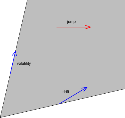
Conditions (1.11)–(1.13) are geometric conditions on the coefficients of the SPDE (1.3); condition (1.11) concerns the behaviour of the solution process in the cone, and conditions (1.12) and (1.13) concern the behaviour of the solution process at boundary points of the cone:
-
•
Condition (1.11) is a condition on the jumps; it means that the cone is invariant for the functions for -almost all .
-
•
Condition (1.12) means that the drift is inward pointing at boundary points of the cone.
-
•
Condition (1.13) means that the volatilities are parallel at boundary points of the cone.
Figure 1 illustrates conditions (1.11)–(1.13). Let us provide further explanations regarding the drift condition (1.12). For this purpose, we fix an arbitrary pair . By the definition (1.10) of the set , we have , indicating that we are at the boundary of the cone.
-
•
The drift condition (1.12) implies
(1.14) This means that the jumps of the solution process at boundary points of the cone are of finite variation, unless they are parallel to the boundary.
- •
- •
We refer to Section 2 for the proofs of these and of further statements. We emphasize that for with it may happen that . In this case, conditions (1.12) – and hence (1.14) – and (1.13), the two boundary conditions illustrated in Figure 1, do not need to be fulfilled. Intuitively, at such a boundary point of the cone, there is an infinite drift pulling the process in the interior of the half space , whence we can skip conditions (1.12) and (1.13) in this situation. This phenomenon is typical for SPDEs, as for norm continuous semigroups (in particular, if ) the limes inferior appearing in (1.10) is always finite.
Now, let us outline the essential ideas for the proof of Theorem 1.1:
-
•
In Theorem 3.1 we will prove that conditions (1.11)–(1.13) are necessary for invariance of the cone , where the main idea is to perform a short-time analysis of the sample paths of the solution processes. We emphasize that for this implication we do not need the assumption that is generated by an unconditional Schauder basis; that is, we can skip Assumption 4.2 here.
-
•
In order to show that conditions (1.11)–(1.13) are sufficient for invariance of the cone , we perform several steps:
- (1)
-
(2)
Then, we show that the cone is invariant for diffusion SPDEs (1.6) with Lipschitz coefficients without imposing smoothness on the volatilities; see Theorem 6.1. The main idea is to approximate the volatility by a sequence of smooth volatilities, and to apply a stability result (see Proposition B.3) for SPDEs.
- (3)
-
(4)
Finally, we show that the cone is invariant for the SPDE (1.3) in the general situation, where the coefficients are locally Lipschitz and satisfy the linear growth condition; see Theorem 8.1. This is done by approximating the parameters of the SPDE (1.3) by a sequence of globally Lipschitz coefficients, and to argue by stability. In order to ensure that the modified coefficients also satisfy the required invariance conditions (1.11)–(1.13), the structural properties of closed convex cones are essential.
The most challenging is the second step, where we approximate the volatility by a sequence of smooth volatilities. In particular, for an application of our stability result (Proposition B.3) we must ensure that all are Lipschitz continuous with a joint Lipschitz constant. We can roughly divide the approximation procedure into the following steps:
- (a)
-
(b)
Then, we approximate a bounded volatility with finite dimensional range by a sequence from . This is done by the so-called sup-inf convolution technique from [23]; see Proposition D.28. Although we do not use it in this paper, we mention the related article [22], which shows how a Lipschitz function can be approximated by uniformly Gâteaux differentiable functions.
-
(c)
Finally, we approximate a volatility from by a sequence from ; see Proposition D.38. This is done by a generalization of the mollifying technique in infinite dimension. For this procedure, we follow the construction provided in [15], which constitutes a generalization of a result from Moulis (see [27]), whence we also refer to this method as Moulis’ method. Concerning smooth approximations in infinite dimensional spaces, we also mention the related papers [1, 2, 17, 18].
We emphasize that we cannot directly apply Moulis’ method in step (b), because for a Lipschitz continuous function this would only provide a sequence from – in fact, even – but the second order derivatives might be unbounded. Applying the sup-inf convolution technique before ensures that we obtain a sequence from . We mention that a combination of the sup-inf convolution technique and Moulis’ method has also been used in [1] in order to prove that every Lipschitz continuous function defined on a (possibly infinite dimensional) separable Riemannian manifold can be uniformly approximated by smooth Lipschitz functions.
Besides the aforementioned required joint Lipschitz constant, we have to take care that the respective approximations of the volatility remain parallel at boundary points of the cone; that is, condition (1.13) must be preserved, which is expressed by Definition C.3. The situation is similar for the approximations of the drift . They must remain inward pointing at boundary points of the cone; that is, condition (1.12) must be preserved, which is expressed by Definition C.2.
It arises the problem that we can generally not ensure in steps (b) and (c) that the approximating volatilities remain parallel. In order to illustrate the situation in step (c), where we apply Moulis’ method, let us assume for the sake of simplicity that the state space is . Then the construction of the approximating sequence becomes simpler than in the infinite dimensional situation in [15], and it is given by the well-known construction
where is an appropriate sequence of mollifiers. Then, for , which implies , we generally have
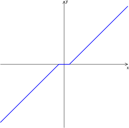
because we only have , but generally not for all from a neighborhood of . This problem leads to the notion of locally parallel functions (see Definition D.1), which have the desired property that for all from an appropriate neighborhood of . In order to implement this concept, we have to show that a parallel function can be approximated by a sequence of locally parallel functions. The idea is to approximate a function for by taking , where
and where the function is defined as
| (1.18) |
see Figure 2. We can also establish this procedure in infinite dimension; see Proposition D.19.
The remainder of this paper is organized as follows. In Section 2 we present the mathematical framework and preliminary results. In Section 3 we prove that our invariance conditions are necessary for invariance of the cone. In Section 4 we provide the required background about closed convex cones generated by unconditional Schauder basis. Afterwards, we start with the proof that our invariance conditions are sufficient for invariance of in the cone. In Section 5 we prove this for diffusion SPDEs with smooth volatilities, in Section 6 for diffusion SPDEs with Lipschitz coefficients without imposing smoothness on the volatility, in Section 7 for general jump-diffusion SPDEs with Lipschitz coefficients, and in Section 8 for the general situation of jump-diffusion SPDEs with coefficients being locally Lipschitz and satisfying the linear growth condition. In Section 9 we provide an example illustrating our main result. In Appendix A we collect the function spaces which we use throughout this paper, and in Appendix B we present the required stability result for SPDEs. In Appendix C we provide the required results about inward pointing functions, and in Appendix D about parallel functions.
2. Mathematical framework and preliminary results
In this section, we present the mathematical framework and preliminary results. Let be a filtered probability space satisfying the usual conditions. Let be a separable Hilbert space and let be the infinitesimal generator of a -semigroup on .
2.1 Assumption.
We assume that the semigroup is pseudo-contractive; that is, there exists a constant such that
| (2.1) |
In view of condition (2.1), we emphasize that for we denote by the Hilbert space norm, and that for a bounded linear operator we denote by the operator norm
Let be a separable Hilbert space, and let be an -valued -Wiener process for some nuclear, self-adjoint, positive definite linear operator ; see [6, pages 86, 87]. There exist an orthonormal basis of and a sequence with such that
Let be a Blackwell space, and let be a homogeneous Poisson random measure with compensator for some -finite measure on ; see [21, Def. II.1.20]. The space , equipped with the inner product
| (2.2) |
is another separable Hilbert space. We denote by the space of all Hilbert-Schmidt operators from into . We fix the orthonormal basis of given by for each , and for each we set for . Furthermore, we denote by the space of all square-integrable functions from into . Let , and be measurable functions. Concerning the upcoming notation, we remind the reader that in Appendix A we have collected the function spaces used in this paper.
2.2 Assumption.
We suppose that
Assumption 2.2 ensures that for each the SPDE (1.3) has a unique mild solution; that is, an -valued càdlàg adapted process , unique up to indistinguishability, such that
| (2.3) | ||||
The sequence defined as
| (2.4) |
is a sequence of real-valued standard Wiener processes, and we can write (2.3) equivalently as
| (2.5) | ||||
Note that Assumption 2.2 is implied by the slightly stronger conditions
Under such global Lipschitz conditions, we refer the reader to [6, 33, 16, 24] for diffusion SPDEs, to [31] for Lévy driven SPDEs, and to [25, 9] for general jump-diffusion SPDEs. Under the local Lipschitz and linear growth conditions from Assumption 2.2, we refer to [36].
2.3 Definition.
2.4 Definition.
A subset is called a cone if we have for all and all .
2.5 Definition.
A cone is called a convex cone if we have for all .
Note that a convex cone is indeed a convex subset of .
2.6 Definition.
A convex cone is called a closed convex cone if it is closed as a subset of .
For what follows, we fix a closed convex cone . Denoting by its dual cone (1.7), the cone has the representation (1.8).
2.7 Definition.
A subset is called a generating system of the cone if we have the representation (1.9).
Of course is a generating system of the cone . However, for applications we will choose the generating system as convenient as possible. In this respect, we mention that, by Lindelöf’s lemma, the cone admits a generating system which is at most countable. For what follows, we fix a generating system .
2.8 Definition.
For a function we say that is -invariant if .
2.9 Definition.
The closed convex cone is called invariant for the semigroup if is -invariant for all .
According to [30, Cor. 1.10.6] the adjoint semigroup is a -semigroup on with infinitesimal generator .
2.10 Lemma.
The following statements are equivalent:
-
(i)
is invariant for the semigroup .
-
(ii)
is invariant for the adjoint semigroup .
Proof.
For , where the constant stems from the growth estimate (2.1), we define the resolvent . We consider the abstract Cauchy problem
| (2.8) |
2.11 Lemma.
The following statements are equivalent:
-
(i)
is invariant for the semigroup .
-
(ii)
is invariant for the abstract Cauchy problem (2.8).
-
(iii)
is -invariant for all .
Proof.
From now on, we make the following assumption.
2.12 Assumption.
We assume that the cone is invariant for the semigroup ; that is, any of the equivalent conditions from Lemma 2.11 is fulfilled.
2.13 Lemma.
For all we have
Proof.
Since is invariant for the semigroup , we have for all , which establishes the proof. ∎
2.14 Definition.
For we write if .
Recall the set defined in (1.10). We define the function
2.15 Lemma.
For each the following statements are true:
-
(1)
We have .
-
(2)
For all we have and
(2.9) -
(3)
For all with we have and
(2.10)
Proof.
For each with we have
and hence
showing that . This proves the first statement, and we proceed with the second statement. Since is a cone, we have . Furthermore, we have
showing and the identity (2.9). For the proof of the third statement, let be arbitrary. By Lemma 2.10 we have . Since , we obtain , and hence
Consequently, we have
| (2.11) |
There exists a sequence with such that the sequence defined as
converges to . Defining the sequence as
by (2.11) we have for each . Hence, the sequence is bounded, and by the Bolzano-Weierstrass theorem there exists a subsequence such that converges to some with , which proves and (2.10). ∎
2.16 Lemma.
Proof.
If , then we have
as , showing the first statement. Furthermore, if , then we obtain
as , showing the second statement. The third statement is an immediate consequence of the first and the second statement. ∎
The following definition is inspired by [26, Lemma 5].
2.17 Definition.
We call a local operator if , and for all we have .
2.18 Proposition.
Suppose that condition (1.11) is fulfilled. Then for all the following statements are true:
-
(1)
We have
-
(2)
We have
- (3)
- (4)
- (5)
- (6)
- (7)
Proof.
By (1.11), for -almost all we have
which establishes the first statement. The second statement is an immediate consequence, and the third statement is obvious. The fourth and the fifth statement follow from Lemma 2.16. Taking into account Definition 2.17, the sixth statement is an immediate consequence of the fifth statement. Finally, the last statement follows from the first statement. ∎
In view of condition (1.15), we emphasize that is dense is , which follows from the next result.
2.19 Lemma.
We have .
Proof.
Since is closed, we have . In order to prove the converse inclusion, let be arbitrary. For we set . Then we have for each , and we have for . It remains to show that for each . For this purpose, let and be arbitrary. Since is invariant for the semigroup , we obtain
showing that . ∎
3. Necessity of the invariance conditions
In this section, we prove the necessity of our invariance conditions.
3.1 Theorem.
Proof.
Condition (1.11) follows from [12, Lemma 2.11]. Let be arbitrary, and denote by the mild solution to (1.3) with . Since the measure space is -finite, there exists an increasing sequence with for each such that . Let be arbitrary. According to [12, Lemma 2.20] the mapping given by
is a strictly positive stopping time. We denote by the mild solution to the SPDE
Since is a closed subset of , by [12, Prop. 2.21] we obtain up to an evanescent set. We define the strictly positive, bounded stopping time
Furthermore, for every stopping time we define the processes and as
Then, by the Cauchy-Schwarz inequality and Assumptions 2.1, 2.2 we have and for each stopping time , where denotes the space of all finite variation processes with integrable variation (see [21, I.3.7]) and denotes the space of all square-integrable martingales (see [21, Def. I.1.41]). Moreover, we have -almost surely
Let be a sequence with such that
| (3.1) |
By Lebesgue’s dominated convergence theorem we obtain
showing that
| (3.2) |
Furthermore, by the monotone convergence theorem and Proposition 2.18 we have
| (3.3) |
Now, suppose that condition (1.13) is not fulfilled. Then there exist and such that . We define by
| (3.4) |
Note that, by (1.12) and Proposition 2.18 we have . The stochastic exponential
where the Wiener process is given by (2.4), is a strictly positive, continuous local martingale. We define the strictly positive, bounded stopping time
For every stopping time we define the processes , and as
Then, by Assumptions 2.1, 2.2 we have and for each stopping time . Moreover, we have -almost surely
Let be an arbitrary stopping time. By [21, Prop. I.4.49] we have , and by [21, Thm. I.4.52] we have . Therefore, and since
by [21, Def. I.4.45] we obtain
| (3.5) | ||||
Let be a sequence with such that we have (3.1). By (3.5), Lebesgue’s dominated convergence theorem and (3.4) we obtain
a contradiction. ∎
4. Cones generated by unconditional Schauder bases
In this section, we provide the required background about closed convex cones generated by unconditional Schauder bases. Let be an unconditional Schauder basis of the Hilbert space ; that is, for each there is a unique sequence such that
| (4.1) |
and the series (4.1) converges unconditionally. Without loss of generality, we assume that for all .
4.1 Remark.
Every orthonormal basis of the Hilbert space is an unconditional Schauder basis. Of course, the converse statement is not true, but for every unconditional Schauder basis of the Hilbert space there is an equivalent inner product on under which the unconditional Schauder basis is an orthonormal basis; see [3].
There are unique elements such that
where we refer to the series representation (4.1); see [7, page 164]. Given these coordinate functionals , we also call an unconditional Schauder basis of . Recall that, throughout this paper, we consider a closed convex cone with representation (1.9) for some generating system . Now, we make an additional assumption on the generating system of the cone.
4.2 Assumption.
We assume there is an unconditional Schauder basis of such that
4.3 Remark.
Equivalently, we could demand . Assumption 4.2 ensures that the generating system becomes minimal.
We define the sequence of finite dimensional subspaces as . Furthermore, we define the sequence of projections as
| (4.2) |
where we refer to the series representation (4.1) of . We denote by the basis constant of the Schauder basis . Since the Schauder basis is unconditional, by [7, Prop. 6.31] there is a constant such for all , all and all we have
| (4.3) |
The smallest possible constant such that the inequality (4.3) is fulfilled, is called the unconditional basis constant, and is denoted by .
4.4 Lemma.
The following statements are true:
-
(1)
We have .
-
(2)
For each we have .
- (3)
Proof.
4.5 Lemma.
The following statements are true:
-
(1)
We have as .
-
(2)
For all , all and all we have
5. Sufficiency of the invariance conditions for diffusion SPDEs with smooth volatilities
In this section, we prove the sufficiency of our invariance conditions for diffusion SPDEs (1.6) with smooth volatilities. Recall that the distance function of the cone is given by
5.1 Lemma.
The following statements are true:
-
(1)
For all and we have
(5.1) -
(2)
For all and we have
(5.2)
Proof.
The following result ensures that the stochastic semigroup Nagumo’s condition (SSNC) is fulfilled in our situation.
5.2 Proposition.
Let be such that for all we have
| (5.3) |
Then, for each we have
| (5.4) |
Proof.
Since , there is an index such that . Let be arbitrary. We set and
Then we have the decomposition , for each there exists such that , and for each there exists such that and . Furthermore, we set for each . There is a sequence with such that
| (5.5) |
where we agree on the notation
Inductively, we define the subsequences for as follows:
-
(1)
For we set for each .
-
(2)
Let be arbitrary, and suppose that we have defined , where denotes the largest integer from with . We distinguish two cases:
-
•
If , then we choose a subsequence of such that for all .
-
•
Otherwise, we choose a subsequence of such that converges to a finite limit for .
-
•
Now, we define the subsequence as for each , where denotes the largest integer from . Furthermore, we define the sets
Then we have the decomposition , and by (5.3) we have
| (5.6) | ||||
| (5.7) |
Since , and is invariant for the semigroup and -invariant, by Lemma 5.1 and (5.5), (5.7), for each we obtain
and by the continuity of the distance function and (5.6) we have
completing the proof. ∎
5.3 Theorem.
Proof.
Condition (5.9) just means that for each the function is weakly locally parallel in the sense of Definition D.2, which allows us to apply Lemma D.9 in the sequel. Let be the function defined in (D.3). According to our hypotheses and Lemma D.8, all assumptions from [29] are satisfied. Let be arbitrary, and define the function as
Since and , we have . Let be arbitrary. Then, by (5.8) and Lemmas D.9, D.10 we deduce that condition (5.3) is fulfilled. Therefore, by Proposition 5.2 the SSNC (5.4) is fulfilled. Consequently, applying [29, Prop. 1.1] yields that the closed convex cone is invariant for the SPDE (1.6). ∎
6. Sufficiency of the invariance conditions for diffusion SPDEs with Lipschitz coefficients
In this section, we prove that our invariance conditions are sufficient for diffusion SPDEs (1.6) with Lipschitz coefficients, without imposing smoothness on the volatility.
6.1 Theorem.
Proof.
For the proof of this result, we will apply the results from Appendices C and D. Note that Assumption C.1 is fulfilled by virtue of Lemma 2.15. Concerning the drift , we use the approximation results from Appendix C as follows:
- (1)
- (2)
- (3)
Furthermore, concerning the volatility , we use the approximation results from Appendix D as follows:
- (1)
- (2)
- (3)
- (4)
- (5)
- (6)
- (7)
Consequently, applying Theorem 5.3 completes the proof. ∎
7. Sufficiency of the invariance conditions for SPDEs with Lipschitz coefficients
In this section, we prove that our invariance conditions are sufficient for general jump-diffusion SPDEs (1.3) with Lipschitz coefficients.
7.1 Theorem.
Proof.
Since the measure is -finite, by our stability result (Proposition B.3) it suffices to prove that for each with the cone is invariant for the SPDE
Moreover, by the jump condition (1.11) and [12, Lemmas 2.12 and 2.20], it suffices to prove that the cone is invariant for the SPDE
| (7.3) |
where is given by
Note that by the Cauchy-Schwarz inequality we have . Let be arbitrary. By (1.12) and Proposition 2.18 we obtain
Therefore, applying Theorem 6.1 yields that the cone is invariant for the SPDE (7.3), completing the proof. ∎
8. Sufficiency of the invariance conditions and proof of the main result
In this section, we prove that our invariance conditions are sufficient for jump-diffusion SPDEs (1.6) with coefficients being locally Lipschitz and satisfying the linear growth condition.
8.1 Theorem.
Proof.
Let be arbitrary. Let be the sequence of retractions defined according to Definition A.9. We define the sequences of functions , and as
Let be arbitrary. Then, by Lemma A.10 we have
and hence, there exists a unique mild solution to the SPDE (B.3) with . Now, we check that conditions (1.11)–(1.13) are fulfilled with replaced by . Following the notation from Definition A.9, there is a function such that
Let be arbitrary. By the properties of the closed convex cone we have and , and hence, since condition (1.11) is satisfied for , we obtain
for -almost all , showing (1.11) with replaced by . Now, let be such that . Then, by Lemma 2.15 we also have , and since condition (1.13) is satisfied for , we obtain
showing (1.13) with replaced by . Furthermore, since condition (1.12) is satisfied for , we obtain
showing (1.12) with replaced by . Consequently, by Theorem 7.1 we have up to an evanescent set. Now, we define the increasing sequence of stopping times by and
Then we have , and the mild solution to (1.3) with is given by
| (8.1) |
showing that up to an evanescent set. ∎
Now, we are ready to provide the proof of our main result, which concludes the paper.
9. An example
In this section, we provide an example illustrating our main result. Let be the Hilbert space consisting of all sequences such that . As in [30, Example 2.5.4], let be the semigroup given by
| (9.1) |
Then is a -semigroup with infinitesimal generator defined on the domain
and given by
We consider the closed convex cone
consisting of all nonnegative sequences.
9.1 Proposition.
Proof.
By definition (9.1) the semigroup is a semigroup of contractions, and the cone is invariant for the semigroup , showing that Assumptions 2.1 and 2.12 are fulfilled. Moreover, the cone is self-dual; that is , and we have the representation
where is given by , showing that Assumption 4.2 is satisfied. Furthermore, for all we have
and in this case the limes inferior vanishes. Consequently, applying Theorem 1.1 completes the proof. ∎
Appendix A Function spaces
In this appendix, we collect the function spaces used in this paper. Let and be two normed spaces.
A.1 Definition.
We introduce the following notions:
-
(1)
For a constant a function is called -Lipschitz if
(A.1) -
(2)
For a constant we define the space
-
(3)
A function is called Lipschitz continuous.
-
(4)
We define the space .
-
(5)
For a constant we define the space .
-
(6)
We define the space .
A.2 Definition.
We introduce the following notions:
-
(1)
A function is called locally Lipschitz if for each there is a constant such that
-
(2)
We denote by the space of all locally Lipschitz functions .
-
(3)
We define the space .
A.3 Definition.
We introduce the following notions:
-
(1)
We say that a function satisfies the linear growth condition if there is a finite constant such that
(A.2) -
(2)
We denote by the space of all functions satisfying the linear growth condition.
-
(3)
We define the space .
A.4 Definition.
We introduce the following notions:
-
(1)
A function is called bounded if there is a constant such that
-
(2)
We denote by the space of all bounded functions .
-
(3)
We define the space .
A.5 Definition.
We introduce the following notions:
-
(1)
A function is called locally bounded if for each there is a constant such that
(A.3) -
(2)
We denote by the space of all locally bounded functions .
-
(3)
We define the space .
Note that . Indeed, if (A.2) is satisfied, for each we set , and then for all with we obtain
showing (A.3).
A.6 Definition.
We introduce the following notions:
-
(1)
We denote by the space of all continuous functions .
-
(2)
We define the space .
-
(3)
We define the spaces and .
Note that . For the next definition, we agree about the convention , where denotes the natural numbers.
A.7 Definition.
Let be arbitrary.
-
(1)
We denote by the space of all -times continuously differentiable functions .
-
(2)
We denote by the space of all such that is bounded and the derivatives , are bounded.
-
(3)
We define the spaces and .
Note that .
A.8 Definition.
We introduce the following notions:
-
(1)
We denote by the space of all such that .
-
(2)
We define the space .
Note that . For the rest of this section, let be a Hilbert space.
A.9 Definition.
For each we define the retraction
where the function is given by
A.10 Lemma.
The following statements are true:
-
(1)
We have as .
-
(2)
For each we have .
Proof.
The first statement directly follows from Definition A.9. For the proof of the second statement, let be arbitrary. Then we have for all , and hence . Furthermore, the ball is a closed convex set. Let and be arbitrary. If , then we have , and hence
Now, suppose that . By the Cauchy Schwarz inequality we have
Moreover, we have , and it follows that
Consequently, the mapping is the metric projection onto the closed convex set , and therefore we have . ∎
Appendix B Stability result for SPDEs
In this appendix, we present the required stability result for SPDEs. The mathematical framework is that of Section 2. Apart from the SPDE (1.3), we consider the sequence of SPDEs given by
| (B.3) |
for each .
B.1 Assumption.
We suppose that the following conditions are fulfilled:
-
(1)
There exists such that , and for all .
-
(2)
We have , and for .
B.2 Proposition.
Proof.
This is a consequence of [9, Prop. 9.1.2]. ∎
B.3 Proposition.
Proof.
Let be arbitrary. We denote by the mild solution to (1.3) with , and for each we denote by the mild solution to (B.3) with . Then, for each there is an event with such that for all . Setting we have and for all and all . Now, let be arbitrary. By Proposition B.2 we have
and hence, there is a subsequence such that -almost surely
Since is closed, there is an event with such that for all . Therefore, setting we obtain and for all , showing that is invariant for (1.3). ∎
Appendix C Inward pointing functions
In this appendix, we provide the required results about inward pointing functions, which we need for the proof of Theorem 6.1. As in Section 2, let be a separable Hilbert space, let be a closed convex cone, and let be a generating system of the cone such that Assumption 4.2 is fulfilled. Let be a subset, and let be a function.
C.1 Assumption.
We suppose that for each the following conditions are fulfilled:
-
(1)
We have .
-
(2)
For all we have and
-
(3)
For all with we have and
C.2 Definition.
Let be a function. We call the pair inward pointing at the boundary of (in short inward pointing) if for all we have
C.3 Definition.
A function is called parallel at the boundary of (in short parallel) if for all we have
C.4 Definition.
Let be a function. Then the set is called -invariant if
C.5 Remark.
Let be a function. If is -invariant, then is parallel.
C.6 Lemma.
Let be a function such that is inward pointing. Then, for each the pair is inward pointing, too.
Proof.
C.7 Definition.
We introduce the following spaces:
-
(1)
For each we denote by the space of all functions .
-
(2)
We set .
C.8 Proposition.
Let be a function such that is inward pointing. Then, there are a constant and a sequence
| (C.1) |
such that is inward pointing for each , and we have .
Proof.
C.9 Lemma.
Let be two functions such that the following conditions are fulfilled:
-
(1)
is inward pointing.
-
(2)
is -invariant, and for all we have
(C.2)
Then the pair is inward pointing.
Proof.
Let be arbitrary. Since the set is -invariant, we have . Therefore, by (C.2), and since is inward pointing, we obtain
finishing the proof. ∎
We denote the retractions defined according to Definition A.9. We will need the following auxiliary result.
C.10 Lemma.
Let be arbitrary. Then is -invariant, and for all we have
Proof.
C.11 Proposition.
Let be a function such that is inward pointing. Then there are a constant and a sequence
| (C.3) |
such that is inward pointing for each , and we have .
Appendix D Parallel functions
In this appendix, we provide the required results about parallel function, which we need for the proofs of Theorems 5.3 and 6.1. The general mathematical framework is that of Appendix C. First, we will extend the Definition C.3 of a parallel function.
D.1 Definition.
A function is called locally parallel to the boundary of (in short locally parallel) if there exists such that for all we have
| (D.1) |
D.2 Definition.
A function is called weakly locally parallel to the boundary of (in short weakly locally parallel) if for all there exists such that we have (D.1).
D.3 Definition.
Let be a function. Then the set is called locally -invariant if there exists such that for all we have
D.4 Remark.
Let be a function.
-
(1)
If is locally parallel, then it weakly locally parallel, too.
-
(2)
If is locally -invariant, then is locally parallel.
As in Section 2, let be a separable Hilbert space, and let be a nuclear, self-adjoint, positive definite linear operator. Recall that equipped with the inner product (2.2) is another separable Hilbert space, and that denotes the space of Hilbert-Schmidt operators from into . Furthermore, recall that we have fixed an orthonormal basis of , and that for each we set for . With this notation, the Hilbert-Schmidt norm is given by
| (D.2) |
D.5 Definition.
We denote by the space of all functions such that for some we have for all .
D.6 Definition.
We denote by the space of all functions such that for some index we have for all with .
D.7 Remark.
D.8 Lemma.
Let be arbitrary. Then the following statements are true:
-
(1)
For each we have .
-
(2)
The function defined as
(D.3) belongs to .
Proof.
By assumption, there exists a constant such that
Furthermore, there exists an index such that for all and all with . Noting that for each the norm of the linear operator , is bounded by , by the chain rule and the Cauchy Schwarz inequality, for each we obtain
proving the first statement and . For the proof of the second statement, let be arbitrary. By the chain rule and Cauchy Schwarz inequality we obtain
and hence
showing that . ∎
D.9 Lemma.
Let be such that for each the function is weakly locally parallel. Then the function defined in (D.3) is parallel.
Proof.
Let be arbitrary. Furthermore, let be arbitrary. Since is locally parallel, there exists such that
We define as
Then we have
Therefore, we obtain
This implies
showing that is parallel. ∎
D.10 Lemma.
Let be such that for each the function is parallel. Then, for each the function is parallel.
Proof.
Recall that we have fixed an orthonormal basis of . Let be arbitrary, and let be arbitrary. Since for each the function is parallel, we obtain
showing that is parallel. ∎
For each let be the finite dimensional subspace , denote by the corresponding projection
and let be the linear operator given by for each . Note that for each and each we have
| (D.4) |
D.11 Lemma.
The following statements are true:
-
(1)
For each we have .
-
(2)
For each we have as .
Proof.
D.12 Proposition.
Let be such that for each the function is parallel. Then there are a constant and a sequence
| (D.5) |
such that for all the function is parallel, and we have .
Proof.
D.13 Lemma.
Let be a parallel function. Then, for each the function is parallel, too.
Proof.
In view of the following results, recall the Definition C.7 of .
D.14 Proposition.
Let be a parallel function. Then there are a constant and a sequence
| (D.6) |
such that is parallel for each , and we have .
Proof.
D.15 Lemma.
Let be two functions such that the following conditions are fulfilled:
-
(1)
is parallel.
-
(2)
is -invariant.
Then is parallel.
Proof.
Let be arbitrary. Then we have , because is -invariant. Therefore, and since is parallel, we obtain
finishing the proof. ∎
D.16 Proposition.
Let be a parallel function. Then there are a constant and a sequence
| (D.7) |
such that is parallel for each , and we have .
Proof.
D.17 Lemma.
Let be two functions such that the following conditions are fulfilled:
-
(1)
is parallel.
-
(2)
is locally -invariant.
Then is locally parallel.
Proof.
By assumption, there exists such that for all we have
Let be arbitrary. Since is parallel, we obtain
completing the proof. ∎
For let be the function given by (1.18); see Figure 2. Then we have and
| (D.8) | ||||
| (D.9) | ||||
| (D.10) | ||||
| (D.11) |
Furthermore, for each we have
| (D.12) | ||||
| (D.13) |
D.18 Lemma.
There exist a constant and a sequence such that for each the set is locally -invariant, and we have .
Proof.
We set . Let be arbitrary. We define the function
| (D.14) |
where we refer to the series representation (4.1) of . Let be arbitrary. We define the sequence as
By (D.11) we have for all , and by Lemma 4.4 we obtain
showing that . Let be arbitrary. Then, by (D.10) we obtain
showing that . Let be arbitrary. In order to show that is locally -invariant, we set . Let be arbitrary, and let with be arbitrary. We will show that . For this purpose, let be arbitrary. Since , by Lemma 4.4 we have
| (D.15) |
Since , we have , and hence, we obtain
| (D.16) |
By Assumption 4.2 we have for some and some . Thus, by the definition (D.14) of and relations (D.16) and (D.12) we deduce
showing that . Furthermore, noting that , by the definition (D.14) of and relations (D.15) and (D.13) we obtain
showing that , and hence . By Assumption C.1 we deduce that , showing that is locally -invariant. ∎
D.19 Proposition.
Let be a parallel function. Then there are a constant and a sequence
| (D.17) |
such that is locally parallel for each , and we have .
Proof.
For our next step, we apply the sup-inf convolution technique from [23].
D.20 Definition.
Let be arbitrary.
-
(1)
For each we define
-
(2)
For each we define
D.21 Remark.
Let and be arbitrary. A straightforward calculation shows that
Therefore, the function is also called sup-inf convolution.
D.22 Definition.
Let be arbitrary.
-
(1)
For each we define as
-
(2)
For each we define as
-
(3)
For all we define as
D.23 Lemma.
Let be arbitrary. Then, for each there are such that for all and with we have
Proof.
This follows from the theorem on pages 260, 261 in [23]; in particular relation (12) therein. ∎
D.24 Lemma.
There is a constant such that for all and all we have for each .
Proof.
Setting , this is an immediate consequence of Lemma 4.4. ∎
D.25 Lemma.
Let and be such that for all , where . Then we have .
Proof.
For all we have
completing the proof. ∎
D.26 Lemma.
There exists a constant such that for all , all and all with we have
where .
Proof.
D.27 Lemma.
Let be a locally parallel function. Then the following statements are true:
-
(1)
There exists such that is locally parallel for each .
-
(2)
There exists such that is locally parallel for each .
-
(3)
There exist such that is locally parallel for all and with .
Proof.
Since is locally parallel, there exists such that for all we have (D.1). Furthermore, since , there exists a finite constant such that
| (D.18) |
We define the constants as
Let be arbitrary. We will show that is locally parallel. For this purpose, let be arbitrary. By Assumption 4.2 there exist and such that . Let with be arbitrary. We define the function
Then we have
| (D.19) |
Indeed, by (D.1) we have , and hence . In order to show that , let be arbitrary. We distinguish two cases:
-
•
Suppose that . Since , by (D.1) we have , showing .
- •
Consequently, we have (D.19), and thus, we obtain
showing that is locally parallel. This provides the proof of the first statement. The proof of the second statement is analogous, and the third statement follows from the first and the second statement. ∎
D.28 Proposition.
Let be a locally parallel function. Then there are a constant and a sequence
such that is locally parallel for each , and we have .
For our last step, we use Moulis’ method, as presented in [15]. For this purpose, we introduce some notation. Let be a smooth function such that the following conditions are fulfilled:
-
•
We have for all .
-
•
We have for all with .
-
•
We have for all .
-
•
We have for all .
Let be arbitrary. We fix a sequence and a constant . We define the sequence of functions as
| (D.20) |
where the sequence is given by
| (D.21) |
D.29 Lemma.
The following statements are true:
-
(1)
We have for each .
-
(2)
There is a constant such that
(D.22) for all and all .
Proof.
Now, we define the sequence of functions as
| (D.23) |
where the sequence is chosen large enough such that
| (D.24) |
for all and all . Inductively, we define the sequence of functions by
| (D.25) | ||||
| (D.26) |
D.30 Lemma.
The following statements are true:
-
(1)
We have and for all .
-
(2)
There is a constant such that
(D.27) for all and all .
Proof.
Now, we define as
| (D.28) |
where . In view of Lemma D.30, we have
| (D.29) |
Now, we define the function
| (D.30) |
where we refer to the series representation (4.1) of , and where for each the function is given by
| (D.31) |
where denotes the linear operator
| (D.32) |
with denoting the constant from above.
D.31 Lemma.
The following statements are true:
-
(1)
We have .
-
(2)
For each there exist and such that
(D.33)
Proof.
This follows from [2, page 17]. ∎
Now, we define the function
| (D.34) |
Note that we emphasize the dependence on the sequences and , and on the constant . For two sequences and we agree to write if for all .
D.32 Lemma.
Let be arbitrary. Then, for each there are sequences , where is chosen such that (D.24) is fulfilled with replaced by , and a constant such that for all sequences with and and all with we have
Proof.
This follows from [15, Thm. 1] and its proof. ∎
D.33 Lemma.
There exists a constant such that for all , all and all sequences , where is chosen such that (D.24) is fulfilled, and every constant we have
where .
Proof.
Lemma D.33 does not ensure that ; that is, it remains to show that the second order derivative is bounded. For this purpose, we prepare some auxiliary results. For the next two results, we fix a constant . Note that the functions , defined in (D.31) and defined in (D.30) depend on the choice of .
D.34 Lemma.
The following statements are true:
-
(1)
We have for each .
-
(2)
There is a constant such that
(D.35) for all and all .
Proof.
Let be the open set . For the norm function given by we have with derivatives
Therefore, for all we obtain
| (D.36) |
We define the constant as
Then, by the definition (D.32) of we have
| (D.37) |
There is a constant such that
Now, we define the constant as
Let be arbitrary. By the definition (D.31) of we have
and hence
We define the open sets as
Then we have and for all . This shows , proving the first statement, and regarding the second statement, it suffices to show (D.35) for all and all . Let and all be arbitrary. By (D.36) and (D.37) we obtain
and hence
completing the proof. ∎
The following auxiliary result extends Fact 7 in [2].
D.35 Lemma.
There exists a constant such that
| (D.38) |
Proof.
Let be the constant from Lemma D.34. We define the constant as
Let be arbitrary. Noting that for , let be the smallest index such that
| (D.39) |
Then we have for all . By the continuity of the linear operators , there exists such that
By the definition (D.31) of we obtain
and it follows that
| (D.40) |
Furthermore, by the definition (D.30) of we have
and hence, by (D.40), Lemmas 4.4, D.34 and (D.39) we obtain
and similarly
completing the proof. ∎
D.36 Lemma.
For all and all sequences , where is chosen such that (D.24) is fulfilled, and every constant we have .
Proof.
By Lemmas D.30 and D.35 there exist constants such that we have (D.27) and (D.38). Let be arbitrary. By Lemma D.31 there exist and such that we have (D.33). Furthermore, by the definition (D.34) of and relation (D.29) we have
Therefore, and by estimates (D.27) and (D.38), we obtain
finishing the proof. ∎
D.37 Lemma.
Let be a locally parallel function. Then, there exist a sequences , where is chosen such that (D.24) is fulfilled with replaced by , such that for all sequences with and and every constant the function is weakly locally parallel.
Proof.
Since is locally parallel, there exists such that for all we have (D.1). Let be the sequence given by for each . Furthermore, we choose such that for each , and condition (D.24) is fulfilled with replaced by . Let be arbitrary sequences with and , and let be an arbitrary constant. First, we will show that for all and all we have
| (D.41) |
For this purpose, let with be arbitrary. By the definition (D.20) of , relation (D.1), and since and , we obtain
showing (D.41). Noting the definition (D.23) of , relation (D.41) and that , analogously we show that for all and all we have
| (D.42) |
Next, we set . By induction, we will show that for all and all we have
| (D.43) |
Relation (D.43) holds true for . Indeed, since and , by Assumption C.1 we also have . Therefore, by the definition (D.25) of , and since is parallel, for all with we obtain
For the induction step, suppose that (D.43) is satisfied for . Since and , by Assumption C.1 we also have . Let with be arbitrary. Then, we have
and hence, by the definition (D.26) of , relation (D.42) and the induction hypothesis, we obtain
proving (D.43). Now, let be arbitrary. By the definition (D.30) of we have and , and hence, by Assumption C.1 we also have . By Lemma D.31 there exist and such that we have (D.33), and there exists such that
We define as
Let with be arbitrary. Then we have
and hence, by the definition (D.34) of , relation (D.29) and (D.43) we obtain
showing that is weakly locally parallel. ∎
D.38 Proposition.
Let be a locally parallel function. Then there are a constant and a sequence
such that is weakly locally parallel for each , and we have .
References
- [1] Azagra, D., Ferrera, J., López-Mesas, F., Rangel, Y. (2007): Smooth approximation of Lipschitz functions on Riemannian manifolds. Journal of Mathematical Analysis and Applications 124(1), 47–66.
- [2] Azagra, D., Gil, J. G., Jaramillo, J. A., Lovo, M. (2005): -fine approximation of functions on Banach spaces with unconditional basis. The Quarterly Journal of Mathematics 56(1), 13–20.
- [3] Bari, N. K. (1951): Biorthogonal systems and bases in Hilbert Space. Uch. Zap. Mosk. Gos. Univ. 148, 69–107.
- [4] Björk, T., Landén, C. (2002): On the construction of finite dimensional realizations for nonlinear forward rate models. Finance and Stochastics 6(3), 303–331.
- [5] Björk, T., Svensson, L. (2001): On the existence of finite dimensional realizations for nonlinear forward rate models. Mathematical Finance 11(2), 205–243.
- [6] Da Prato, G., Zabczyk, J. (1992): Stochastic equations in infinite dimensions. Cambridge University Press, New York.
- [7] Fabian, M., Habala, P., Hájek, P., Santalucía, V. M., Pelant, J., Zizler, V. (2001): Functional analysis and infinite dimensional geometry. Springer, New York.
- [8] Filipović, D. (2000): Invariant manifolds for weak solutions to stochastic equations. Probability Theory and Related Fields 118(3), 323–341.
- [9] Filipović, D., Tappe, S., Teichmann, J. (2010): Jump-diffusions in Hilbert spaces: Existence, stability and numerics. Stochastics 82(5), 475–520.
- [10] Filipović, D., Tappe, S., Teichmann, J. (2010): Term structure models driven by Wiener processes and Poisson measures: Existence and positivity. SIAM Journal on Financial Mathematics 1(1), 523–554.
- [11] Filipović, D., Tappe, S., Teichmann, J. (2014): Invariant manifolds with boundary for jump-diffusions. Electronic Journal of Probability 19(51), 1–28.
- [12] Filipović, D., Tappe, S., Teichmann, J.: Stochastic partial differential equations and submanifolds in Hilbert spaces. Appendix of Invariant manifolds with boundary for jump-diffusions, (2014). (http://arxiv.org/abs/1202.1076v2)
- [13] Filipović, D., Teichmann, J. (2003): Existence of invariant manifolds for stochastic equations in infinite dimension. Journal of Functional Analysis 197(2), 398–432.
- [14] Filipović, D., Teichmann, J. (2004): On the geometry of the term structure of interest rates. Proceedings of The Royal Society of London. Series A. Mathematical, Physical and Engineering Sciences 460(2041), 129–167.
- [15] Fry, R. (2006): Approximation by -smooth Lipschitz functions on Banach spaces. Journal of Mathematical Analysis and Applications 315(2), 599–605.
- [16] Gawarecki, L., Mandrekar, V. (2011): Stochastic differential equations in infinite dimensions with applications to SPDEs. Springer, Berlin.
- [17] Hájek, P., Johanis, M. (2009): Uniformly Gâteaux smooth approximation on . Journal of Mathematical Analysis and Applications 350(2), 623–629.
- [18] Hájek, P., Johanis, M. (2010): Smooth approximations. Journal of Functional Analysis 259(3), 561–582.
- [19] Jachimiak, W. (1997): A note on invariance for semilinear differential equations. Bulletin of the Polish Academy of Sciences 45(2).
- [20] Jachimiak, W. (1998): Stochastic invariance in infinite dimension. Polish Academy of Sciences.
- [21] Jacod, J., Shiryaev, A. N. (2003): Limit theorems for stochastic processes. Springer, Berlin.
- [22] Johanis, M. (2003): Approximation of Lipschitz mappings. Serdica Mathematical Journal 29(2), 141–148.
- [23] Lasry, J. M., Lions, P. L. (1986): A remark on regularization in Hilbert spaces. Israel Journal of Mathematics 55(3), 257–266.
- [24] Liu, W., Röckner, M. (2015): Stochastic partial differential equations: An introduction Springer, Heidelberg.
- [25] Marinelli, C., Prévôt, C., Röckner, M. (2010): Regular dependence on initial data for stochastic evolution equations with multiplicative Poisson noise. Journal of Functional Analysis 258(2), 616–649.
- [26] Milian, A. (2002): Comparison theorems for stochastic evolution equations. Stochastics and Stochastic Reports 72(1–2), 79–108.
- [27] Moulis, N. (1971): Approximation de fonctions différentiables sur certains espaces de Banach. Ann. Inst. Fourier (Grenoble) 21(4), 293–345.
- [28] Nakayama, T. (2004): Support theorem for mild solutions of SDE’s in Hilbert spaces. J. Math. Sci. Univ. Tokyo 11(3), 245–311.
- [29] Nakayama, T. (2004): Viability Theorem for SPDE’s including HJM framework. J. Math. Sci. Univ. Tokyo 11(3), 313–324.
- [30] Pazy, A. (1983): Semigroups of linear operators and applications to partial differential equations. Springer, New York.
- [31] Peszat, S., Zabczyk, J. (2007): Stochastic partial differential equations with Lévy noise. Cambridge University Press, Cambridge.
- [32] Platen, E., Tappe, S. (2015): Real-world forward rate dynamics with affine realizations. Stochastic Analysis and Applications 33(4), 573–608.
- [33] Prévôt, C., Röckner, M. (2007): A concise course on stochastic partial differential equations. Springer, Berlin.
- [34] Tappe, S. (2010): An alternative approach on the existence of affine realizations for HJM term structure models. Proceedings of The Royal Society of London. Series A. Mathematical, Physical and Engineering Sciences 466(2122), 3033–3060.
- [35] Tappe, S. (2012): Existence of affine realizations for Lévy term structure models. Proceedings of The Royal Society of London. Series A. Mathematical, Physical and Engineering Sciences 468 (2147), 3685–3704.
- [36] Tappe, S. (2012): Some refinements of existence results for SPDEs driven by Wiener processes and Poisson random measures. International Journal of Stochastic Analysis, vol. 2012, Article ID 236327, 24 pages.
- [37] Tappe, S. (2015): Existence of affine realizations for stochastic partial differential equations driven by Lévy processes. Proceedings of The Royal Society of London. Series A. Mathematical, Physical and Engineering Sciences 471(2178).
- [38] Tappe, S. (2016): Affine realizations with affine state processes for stochastic partial differential equations. Stochastic Processes and Their Applications 126(7), 2062–2091.