The dipolar spin glass transition in three dimensions

Abstract

Dilute dipolar Ising magnets remain a notoriously hard problem to tackle both analytically and numerically because of long-ranged interactions between spins as well as rare region effects. We study a new type of anisotropic dilute dipolar Ising system in three dimensions [Phys. Rev. Lett. 114, 247207 (2015)] that arises as an effective description of randomly diluted classical spin ice, a prototypical spin liquid in the disorder-free limit, with a small fraction $x$ of non-magnetic impurities. Metropolis algorithm within a parallel thermal tempering scheme fails to achieve equilibration for this problem already for small system sizes. Motivated by previous work [Phys. Rev. X 4, 041016 (2014)] on uniaxial random dipoles, we present an improved cluster Monte Carlo algorithm that is tailor-made for removing the equilibration bottlenecks created by clusters of effectively frozen spins. By performing large-scale simulations down to $x=1/128$ and using finite size scaling, we show the existence of a finite-temperature spin glass transition and give strong evidence that the universality of the critical point is independent of $x$ when it is small. In this $x\ll 1$ limit, we also provide a first estimate of both the thermal exponent, $\nu=1.27(8)$, and the anomalous exponent, $\eta=0.228(35)$.

Introduction: The term “spin glass” was originally coined to describe dilute magnetic alloys like AuFe CannellaM72 composed of non-magnetic metals (like Au) weakly diluted with magnetic impurities (like Fe) where the impurity spins interact with an RKKY exchange RKKY . Since then, glassy behaviour of spins has been realized in a variety of magnetic systems BinderY86 and the general wisdom is that both frustration and disorder are necessary ingredients for glassiness. Most theoretical studies have focused on Edwards-Anderson type models EdwardsA75 where the spin interactions are short-ranged and random in sign. Extensive numerical simulations have now established the presence of a finite-temperature spin glass transition for Ising spins in three dimensions and its associated critical exponents have been accurately computed  EAnumerics1 ; EAnumerics2 . Such Ising systems are, however, experimentally rare where it is much more common to have Heisenberg spins BinderY86 ; Mydoshbook . With these isotropic degrees of freedom, the nature of the transition is still controversial in the corresponding Edwards-Anderson model vectormodelnumerics1 ; vectormodelnumerics2 ; vectormodelnumerics3 ; vectormodelnumerics4 .

Disordered dipolar Ising magnets such as LiHo_xY_1-xF₄ provide another class of candidate systems review_lithium , qualitatively distinct from their short-ranged counterparts, where the twin ingredients of frustration (due to the nature of the magnetostatic dipole-dipole interaction) and disorder (in the spatial arrangement of the magnetic ions like Ho³⁺ when randomly substituted by non-magnetic Y³⁺ ions) are both present. Experiments have found a spin glass phase for $x<x_{c}$ ReichEYRAB90 where $x_{c}\approx 0.25$ at low temperature. An analysis of the ac susceptibility shows that a spin glass phase may exist even at extreme dilutions of $x=0.045$ QuilliamMMK08 suggesting that a finite-temperature spin glass phase may extend all the way from $x_{c}$ down to $x\rightarrow 0^{+}$.

However, unlike their short-ranged counterparts, the nature of the spin glass ordering in dilute dipolar Ising systems has been a long-standing open issue as conventional analytical and numerical techniques suffer different problems, particularly in the high dilution limit. Mean-field theory suggests that the spin glass order is maintained even in the high-dilution limit, with the critical temperature being linear in the concentration of the spins StephenA81 ; XuBNR91 . However, at high dilution, spatial inhomogeneities are large and could easily modify the mean-field theory predictions. In numerical simulations, long equilibration times severely limit the studied system sizes and concentrations. Even in experiments, equilibration is difficult to achieve due to ultraslow dynamics above the transition temperature (which may be around $10^{7}$ slower than in short-ranged spin glass materials BiltmoH12 ). Due to these difficulties, even the existence of the spin glass transition in such magnets has been a matter of long-standing debate DSG1 ; DSG2 ; DSG3 ; DSG4 . Recent large-scale numerical simulations have shown a spin glass phase down to experimentally relevant low concentrations Gingras ; AndresenKOS14 . The universality class of the highly dilute dipolar Ising magnet in three dimensions, though, is still unknown.

In this work, we study a different, experimentally motivated, example of an emergent dilute anisotropic dipolar system that arises on weakly diluting dipolar spin ice materials on the three dimensional pyrochlore lattice of corner-sharing tetrahedra with non-magnetic impurities, e.g., Dy_2-xY_xTi₂O₇/Ho_2-xY_xTi₂O₇, where the magnetic Dy³⁺/Ho³⁺ ions are replaced randomly by non-magnetic Y³⁺ ions KeFULDCMS07 ; LinKTSMG14 . The disorder-free problem is known to exhibit a topological Coulomb phase CastelnovoMS12 characterised by several non-trivial features like a pinch-point motif in the spin structure factor IsakovGMS04 ; Henley05 ; SenMS13 , large residual entropy of the spins at low temperature RamirezHCSS99 and emergent magnetic monopoles CastelnovoMS08 . In the weak dilution limit ($x\ll 1$), it was shown in Ref. SenM15, that the dense but disordered network of Ising spins can be mapped to a dilute network of emergent Ising spins (dubbed ghost spins) that reside on the sites of the missing spins, have the same local Ising easy axes as the corresponding missing spins (the cubic symmetry of the pyrochlore lattice does not allow collinear Ising axes; rather, each spin points along the line joining the centres of two connected tetrahedra), and are again coupled by a magnetostatic dipole-dipole interaction but with a renormalised coupling constant. We note that, statistically, this model retains the full cubic symmetry of the pyrochlore lattice.

We perform large-scale numerical simulations of this effective dilute dipolar magnetic system using an improved version of a cluster algorithm used in Ref. AndresenKOS14, (the basic idea was also introduced previously in Refs. JanzenHE08, ; AndresenJK11, ) to establish the presence of a finite-temperature spin glass transition. Our algorithm differs from Ref. AndresenKOS14, both in the definition of a cluster and in the relative importance associated to different clusters during a Monte Carlo step. We comment on the relation of our cluster construction to dynamically frozen spin clusters. We also discuss the manner in which the efficiency of the algorithm may be controlled by tuning the cluster construction parameters since it is not rejection-free (unlike Swendsen-Wang SW and Wolff Wolff algorithms for unfrustrated spin models).

Using our cluster algorithm, we have reached total number of spins, $N$, that are roughly twice as large compared to the previous large-scale simulations of related uniaxial Ising systems AndresenKOS14 (note that the CPU time increases quadratically with $N$ for every Monte Carlo sweep of the system owing to long-ranged interactions between the spins). When $x\ll 1$, this problem provides a different lattice realization of (presumably) the same universal physics of the spin glass transition as uniaxial Ising spins interacting via a dipolar coupling in the dilute limit. Using finite-size scaling, we show that $T_{x}\propto x$ and the universality class of the transition is independent of $x$ when it is small. The study of this model enables us to provide an estimate of both the thermal exponent $\nu$ and the anomalous exponent $\eta$ at small $x$ unlike the unixial dipolar model studied earlier in Refs. Gingras, ; AndresenKOS14, (where only $\nu$ could be reliably estimated).

The Model: In dipolar spin ice, the Ising spins on the pyrochlore lattice have local easy axis directions, $\hat{e}_{i}$, that are defined by the line joining the centers of the pair of tetrahedra which share them. The simplest appropriate interaction Hamiltonian of Ising spins with moments $\vec{\mu}_{i,j}$ of size $\mu$, separated by $r_{ij}$, contains short-range exchange interactions in addition to the usual magnetic dipolar term, $D{\cal D}_{ij}$, of strength $D$,with

$${\cal D}_{ij}=\frac{1}{\mu^{2}}\left(\frac{a}{r_{ij}}\right)^{3}\left(\vec{\mu}_{i}\cdot\vec{\mu}_{j}-3(\vec{\mu}_{i}\cdot\hat{r}_{ij})(\vec{\mu}_{j}\cdot\hat{r}_{ij})\right)$$ (1)

where $a$ is the nearest neighbor distance on the pyrochlore lattice CastelnovoMS12 .

Following Ref. SenM15, , a weakly diluted system of spins can be mapped to a highly diluted system of emergent ghost spins. The pairwise interaction between the ghost spins, $\tilde{\cal H}_{ij}$ has the standard dipolar form $\tilde{{\cal H}}_{ij}=\tilde{D}{\cal D}_{ij}$ where $\tilde{D}$ is the effective dipolar coupling constant between the ghost spins which has an entropic contribution coming from the fluctuations of the spins in the bulk SenM15 on top of the simple magnetostatic coupling constant $D$:

$$\tilde{D}=D+\frac{3T}{\sqrt{2}\pi}$$ (2)

Henceforth, we will consider the dipolar coupling constant to be set to $D$=1.41 K (as in Ho₂Ti₂O₇ and Dy₂Ti₂O₇  Sc294_2001 ). The renormalization of $D$ to $\tilde{D}$ simply renormalizes the transition temperature to be $T_{c}(x)=T_{x}/(1-\frac{3T_{x}}{\sqrt{2}\pi})$ where $T_{x}$ is the transition temperature with the coupling set to be $D$. Here $x$ denotes the density of the ghost spins (which is assumed to be small). Thus, the Hamiltonian $\mathcal{H}$ that is studied numerically in this work has the form:

$${\cal H} = D\sum_{i,j(i>j)}\left[\left(\frac{a}{r_{ij}}\right)^{3}\left(\hat{e}_{i}\cdot\hat{e}_{j}-3(\hat{e}_{i}\cdot\hat{r}_{ij})(\hat{e}_{j}\cdot\hat{r}_{ij})\right)\right]S_{i}S_{j}$$ (3)

$$= \sum_{i,j(i>j)}J_{ij}S_{i}S_{j}$$

where $\mu_{i}=\mu S_{i}\hat{e}_{i}$ with $S_{i}=\pm 1$. The long-ranged nature of the dipolar interactions is treated using the Ewald summation technique Ewald without a demagnetization factor.

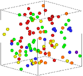
(a) $T=0.072\approx 2T_{x}$

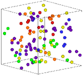
(b) $T=0.047\approx 1.3T_{x}$

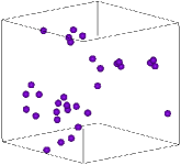
(c) $C_{2}$

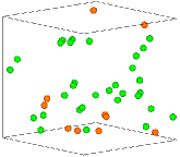
(d) $C_{1},C_{0}$

Figure 1: A particular disorder realization for $L=6$ and $x=1/32$. Colors at different sites in (a) and (b) represent different acceptance ratios of spin flips ($R_{i}$) using a conventional single spin-flip Metropolis algorithm. Sites with $(0<R<10^{-4})$ are denoted by violet, $(10^{-4}<R<10^{-3})$ by blue, $(10^{-3}<R<10^{-2})$ by green, $(10^{-2}<R<0.1)$ by yellow, $(0.1<R<0.25)$ by orange and $(0.25<R<1)$ by red. With the chosen cluster parameters ($a_{s}=1.3125$, $b_{s}=0.75$ and $C_{L}=N/5$), three cluster sets $C_{0}$, $C_{1}$ and $C_{2}$ are obtained for this disorder realization. (c) shows the member sites of the clusters that belong to the set $C_{2}$ (in violet). (d) shows the additional member sites of the clusters in $C_{1}$ that are already not part of $C_{2}$ (in green) and the additional member sites of the clusters in $C_{0}$ that are already not part of $C_{2}$, $C_{1}$(in orange). The figures were generated using the graphics software QMGA software .

Dynamic heterogeneity: Monte-Carlo simulations with a single-spin flip Metropolis algorithm in combination with parallel tempering in temperature HukushimaN96 is the method of choice to simulate Edwards-Anderson type models EAnumerics1 ; EAnumerics2 . However, this local algorithm fails to equilibrate the Ising system considered in Eq. 3 because of long autocorrelation times except for very small system sizes when $x\ll 1$. Apart from the computational effort scaling as $\mathcal{O}(x^{2}L^{6})$ due to the long-ranged interactions, the other more serious bottleneck to equilibration is the presence of clusters of effectively frozen spins at low temperature under a single spin-flip dynamics. Their presence can be seen by monitoring the acceptance ratio, $R_{i}$, of the spin flips at each site $i$ in a particular disorder realization by performing a simulation using the Metropolis algorithm (without any parallel tempering in temperature). A disorder realization is produced by placing (ghost) spins on a fraction $x$ of sites that are randomly selected comment1 from the $16L^{3}$ sites of the system of linear dimension $L$ (with $16$ sites in the conventional cubic unit cell of the pyrochlore lattice). Fig. 1(a) and Fig. 1(b) show the spatial distribution of $R_{i}$ for a particular disorder realization at $L=6$, $x=1/32$ at two different temperatures, $T=0.072(\approx 2T_{x})$ and $T=0.047(\approx 1.3T_{x})$, respectively. The data for $R_{i}$ has been obtained by averaging over $2000$ different runs where the different initial configurations at a temperature $T$ were equilibrated using our cluster algorithm, after which $10^{6}$ spin-flip attempts (per spin) were made using a Metropolis algorithm. A strong dynamic heterogeneity in the behavior of $R_{i}$ is visible at both temperatures. The spins have a wide range of $R_{i}$ with several spins remaining practically frozen (violet and blue sites in Fig. 1(a), Fig. 1(b)), others having an intermediate $R_{i}$ (green and yellow sites in Fig. 1(a), Fig. 1(b)), and the rest having a high $R_{i}$ (orange and red sites in Fig. 1(a), Fig. 1(b)). These effectively frozen spin clusters make the Metropolis algorithm highly inefficient for such dilute dipolar systems. Parallel tempering in temperature also fails to equilibrate such systems since the clustering effects persist even at temperatures like $T\approx 2T_{x}$ (Fig. 1(a)) and above. Such clustering was also observed previously in a numerical study of the dynamics of uniaxial Ising spins BiltmoH12 interacting via dipolar interactions in a dilute system.

Cluster algorithm: To ameliorate the slow equilibration due to these spin clusters, we present a modified version of a cluster algorithm used in Ref. AndresenKOS14, (see also Refs. JanzenHE08, ; AndresenJK11, ). The key idea is to incorporate correlated multi-spin flips to deal with the dynamically frozen spin clusters. The emergence of these clusters can be understood as follows: While the average distance between spins scale as $r_{av}\sim ax^{-1/3}$ and therefore the average of the magnitude of $|J_{ij}|\sim Dr_{av}^{-3}\sim Dx$ (the average value of $|J_{ij}|$ in a disorder realization is denoted by $J_{av}$ henceforth), which is also the reason behind the expectation that $T_{x}\propto x$ at small $x$, the minimum distance between the spins is fixed by the lattice constant $a$ and is independent of $x$. Therefore, in any given disorder realization at small $x$, there will be spin pairs $(i,j)$ such that $|J_{ij}|$ is much greater than $J_{av}$. Fig. 2(a) shows the distribution of $|J_{ij}|$ in one disorder realization for $L=10$ at $x=1/32$. While $J_{av}\sim 10^{-3}$ in this case, there are several spin pairs for which $|J_{ij}|\gg J_{av}$ with the maximum value of $|J_{ij}|\sim 0.2$. These tightly bound spin pairs will be effectively frozen under a local single-spin flip Metropolis update at temperatures $T\sim\mathcal{O}(T_{x})$ wherever $|J_{ij}|\gg T$. Furthermore, the wide distribution in the values of $|J_{ij}|$ at small $x$ (Fig. 2(a)) due to the power-law nature of the interactions explains the wide spread in the values of $R_{i}$ as seen in Fig. 1(a) and Fig. 1(b) under a local single-spin flip dynamics.

An additional correlated flip of these spin pairs (apart from the usual single-spin flips) satisfying detailed balance may seem to be the cure for this problem. However, there will also be frozen clusters in the system which are bigger than size-$2$ (Fig. 2(b)) and cannot be handled by these pair flips alone. Consider any subset of these tightly bound spin pairs that form a connected cluster (Fig. 2(b)) such that it is possible to get from every site in that cluster to every other site in it through these strong bonds, where a strong bond is set by the condition that $|J_{ij}|\gg T$, then all these spins in the cluster are mutually frozen as well with respect to single-spin flips at $T$. Ignoring the rest of the weak bonds in the system effectively breaks it into these connected clusters of spins. This suggests an immediate low-energy move where all the Ising spins $\{S_{i}\}$ that belong to a cluster are flipped together to $\{-S_{i}\}$ irrespective of the values of these spins relative to each other. In Ref. AndresenKOS14, , the clusters were chosen to be fully connected such that all the $n(n-1)/2$ bonds between the spins of a $n$-spin cluster are strong bonds. However, consider a case where two (or more) fully connected clusters share one or more sites (e.g., two size-$2$ clusters formed by sites $(i,j)$ and $(j,k)$ share a common spin at site $j$ but with $|J_{ik}|$ small enough to be a weak bond). Then flipping all the spins of one such fully connected cluster would not necessarily be a low-energy move since it will only flip a subset of spins of the other one(s). To remedy this, one simply needs to flip all the member spins of these fully connected clusters that share the common site(s) simultaneously but this is the same as flipping a single connected cluster in our approach.

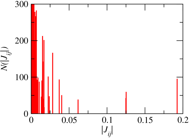
(a)

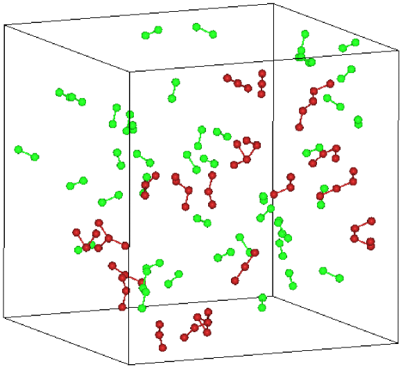
(b)

Figure 2: (a) Variation of the number of bonds, $N(|J_{ij}|)$, with $|J_{ij}|$ for a particular disorder realization at $L=10$ and $x=1/32$. While $J_{av}\sim 10^{-3}$ here, the maximum value of $|J_{ij}|\sim 0.2$. The y axis is truncated at $300$ for clarity. (b) The clusters in the set $C_{n}$ (constructed with the largest $J_{T}$) for a particular disorder realization at $L=10$ and $x=1/32$. The cluster construction parameters used were $a_{s}=1.3125$, $b_{s}=0.75$ and $C_{L}=N/5$. While the majority of the clusters in $C_{n}$ have size-$2$ (indicated in green), there are $n$-spin clusters with $n>2$ as well (indicated in red). Long bonds due to periodic boundary conditions have not been shown here.

Our cluster construction procedure requires specifying three parameters $a_{s}$, $b_{s}$ and $C_{L}$. We then generate different sets of spin clusters for every disorder realization at the beginning of the simulation. We select all the bonds $(i,j)$ where $|J_{ij}|\geq$ $a_{s}J_{av}$ and prepare a list $[(i,j)]$ of the bonds in which their strengths are arranged in ascending order of their magnitudes. We consider the smallest value of $|J_{ij}|$ from this list as $J_{s}$ and initially set $J_{T}=J_{s}$, where $J_{T}$ is a given target energy. We then search for all the bonds $(i,j)$ from the list $[(i,j)]$ such that $|J_{ij}|\geq J_{T}$ and group them into connected clusters. The clusters contain only the site indices and a cluster move is the simultaneous flipping of all its Ising spins $S_{i}$ to $-S_{i}$. Therefore, the flipping of spins during the simulation does not change the definition of the clusters. The collection of clusters for a given $J_{T}$ forms a cluster set. If the size of the largest cluster (i.e., the number of its member spins) in the set exceeds a threshold size $C_{L}$, we reject this cluster set and go to the next higher value in the list $[(i,j)]$ using: $J_{T}\geq J_{T}+\Delta J$ where $\Delta J=b_{s}J_{s}$ which we then use to generate a new set of clusters and again check the size of the largest cluster in it. In this way we sequentially build and reject the sets of clusters until we find a set in which the size of the largest cluster is $\leqslant C_{L}$. We call this set “$C_{0}$”. After the formation of “$C_{0}$”, we form the next set “$C_{1}$” by using only the bonds that have $|J_{ij}|\geq J_{T}$ where $J_{T}\geq J_{T}+\Delta J$ (and $J_{T}$ is again taken from the list $[(i,j)]$). We continue to generate more cluster sets upto the last set of clusters “$C_{n}$” in this manner.

The parameter ‘$a_{s}$’ controls the starting point of cluster constructions for the set $C_{0}$. The requirement is simply to start the construction such that the first ‘test’ set may have at least one cluster of size $>C_{L}$. We consider the parameter ‘$b_{s}$’ to ensure that two successive sets are sufficiently different from each other. $C_{L}$ can be chosen according to the size of the largest frozen cluster (with respect to single spin flips) which clearly increases as the temperature or $x$ is lowered. For most of the simulations, we consider the following parameter values : $a_{s}=1.3125,b_{s}=0.75$ and $C_{L}=N/5$ where $N=16xL^{3}$ is the total number of ghost spins in the respective configurations. The thermalization timescale of the algorithm depends on the parameters $a_{s},b_{s},C_{L}$ but we leave their systematic optimization to a future study (for some discussion, see Appendix A).

Each cluster set contains clusters of different sizes. Each set has a majority of size-$2$ clusters. However, even the final set $C_{n}$ may consist of multiple clusters of size $>2$, especially at large $L$ (See Fig. 2(b)). A small cluster in set $C_{l}$ may well be a part of a larger cluster present in another set $C_{m}$ where $m<l$. A particular cluster may be a member of multiple sets. Going from a cluster set $C_{m}$ to a set $C_{l}$ where $m>l$ entails the following: (a) formation of new clusters not present in $C_{m}$, (b) growth of clusters contained in the set $C_{m}$, and (c) clusters in $C_{m}$ merging to form bigger clusters in $C_{l}$.

The multiple cluster sets $C_{0}$, $\cdots$, $C_{n}$, each with a different $J_{T}$, are constructed since the interaction $J_{ij}$ has a power law nature and thus each disorder realization has a hierarchy of energy scales (Fig. 2(a)). The clusters in the set $C_{n}$ (that has the highest $J_{T}$) mimic the dynamically frozen spin clusters that are formed at higher temperatures (Fig. 1(c)) whereas the clusters in $C_{0}$ mimic frozen spin clusters at lower temperatures (Fig. 1(d)). The member spins of the clusters in set $C_{n}$ are typically composed of spins that have the lowest $R_{i}$ under a local single-spin flip Metropolis algorithm (see Fig. 1(c)). New members of $C_{n-1}$ etc (which do not already belong to the previous sets $C_{n}$ etc) typically have progressively higher values of $R_{i}$ (but still much lower than the spins with the highest values of $R_{i}$ in the system) as can be seen from Fig. 1(d). Our cluster algorithm thus correctly identifies the majority of the frozen spins present in the system at small $x$ as well as the heterogeneity in their dynamic behavior (Fig. 1) by associating them to different sets.

We need to include conventional single-spin flip moves in our cluster algorithm as well not only to keep the Monte Carlo dynamics ergodic (since there are spins which are not part of any cluster) but also for breaking the size-$2$ clusters which is only possible via single spin flips. Similarly, the clusters in a set $C_{m}$ are instrumental in breaking the bigger clusters in a set $C_{l}$ where $m>l$. During our simulation, at each step, we apply either a single spin flip move or a cluster flip move. The probability that a single spin flip is attempted is taken as $85\%$ and that a cluster flip move is attempted is then taken as $15\%$ in most of the simulations. In previous works AndresenKOS14 ; JanzenHE08 ; AndresenJK11 , a cluster was randomly (uniformly) selected from all possible sets and then a cluster flip was attempted. In our approach, each cluster set is assigned a probability of being chosen during the cluster flip move which is taken to be non-uniform, with the highest (lowest) weight given to clusters in $C_{n}$ ($C_{0}$). This way we ensure that the more strongly coupled spins are attempted to be flipped more often.

Specifically, we select the set $C_{n}$ with probability $P_{n}=1/2$, the probability that we select ‘k-th’ set $C_{k}$ is $P_{k}=(1-\sum\limits_{i=k+1}^{n}P_{i})/2$. The probability that we select the set $C_{0}$ is then $P_{0}=$$(1-\sum\limits_{i=1}^{n}P_{i})$. Once a particular cluster set is chosen, then all the clusters of that set have equal probability to be chosen for the actual cluster flip attempt. The relative importance of the different cluster sets in achieving equilibration is discussed further in the Appendix B.

Both the single-spin flips and cluster flips are accepted with the Metropolis probability min$\left[1,\exp(-\Delta E/T)\right]$, where $\Delta E$ is the energy difference between the new configuration and the old configuration, to preserve detailed balance. One Monte-Carlo step (MCS) consists of $N$ spin/cluster flip attempts in total. We further use parallel tempering in temperature HukushimaN96 in combination with the cluster algorithm to accelerate equilibration. In detail, we simulate $2N_{T}$ replicas at $N_{T}$ different temperatures in parallel (thus, two independent replicas at each temperature so that we can calculate overlap observables defined in Eq. 4), with the consecutive temperatures scaled by a factor $c$ such that $T_{n}=(1+c)^{n}T_{0}$, where $n=0,1,2,\cdots,N_{T}-1$ Gingras . The parameters $T_{0},c\mbox{ and }N_{T}$ are adjusted so that the acceptance ratio for parallel tempering swaps between neighbouring temperatures is $>50\%$. For the exchange process, the replica pairs $(T_{m},T_{m+1})$ are divided into two subgroups, i.e., odd-$m$ and even-$m$ groups. The exchange trial is performed for one of these subgroups after every 20 MCS. This sequence which we denote as a Monte Carlo Sweep (MC Sweep) is repeated several times during the course of the simulation. A large number of independent disorder realizations (denoted by $N_{sample}$, which is $1500$ or more) are taken to perform the disorder averaging.

Observables: Let us now describe the observables. The spin glass order parameter, $q_{EA}^{\alpha\beta}(\mathbf{k})$, at wavevector $\mathbf{k}$ is defined as

$$q_{EA}^{\alpha\beta}(\mathbf{k})=\frac{1}{N}\sum_{i}\mu_{i}^{\alpha(1)}\mu_{i}^{\beta(2)}\exp(i\mathbf{k}\cdot\mathbf{r}_{i})$$ (4)

where $\alpha,\beta=x,y,z$ are the spin components (where the ghost spins point along the local easy axes) and $(1)$ and $(2)$ denote two identical disorder realizations of the system with the same set of interactions. From this, we calculate the spin glass susceptibility, $\chi_{SG}(\mathbf{k})$, defined as

$$\chi_{SG}(\mathbf{k})=N\sum_{\alpha,\beta}[\langle|q_{EA}^{\alpha\beta}(\mathbf{k})|^{2}\rangle]$$ (5)

where $\langle\cdots\rangle$ and $[\cdots]$ denote thermal and disorder averages, respectively. In particular, $\chi_{SG}\equiv\chi_{SG}(\mathbf{k}=\mathbf{0})$ is an indicator for the spin glass transition since above (below) the transition, $\chi_{SG}$ is finite (diverges) as $L\rightarrow\infty$. Furthermore, a spin glass correlation length $\xi$ can also be defined by using the following relation:

$$\xi=\frac{1}{2\sin\left(\frac{|\mathbf{k}_{\rm min}|}{2}\right)}\left(\frac{\chi(\mathbf{k}=\mathbf{0})}{\chi(\mathbf{k}_{\rm min})}-1\right)^{\frac{1}{2}}$$ (6)

where $\mathbf{k}_{\rm min}=\frac{2\pi}{L}(1,0,0)$. The ratio $\xi/L$ approaches a universal value characteristic of the critical point as $L\rightarrow\infty$ in case the spin glass transition is continuous in nature.

Equilibration test and autocorrelation time analysis: To test the equilibration of the algorithm, we measure $q_{EA}^{\alpha\beta}(\mathbf{k}=\mathbf{0})$ using a double replica (DR) (Eq. 4) and a single replica (SR) estimator and calculate $\chi_{SG}$ using Eq. 5. The estimators are as follows:

$$q_{DR}^{\alpha\beta}(t_{0}) =\frac{1}{Nt_{0}}\sum_{t=1}^{t_{0}}\sum_{i}\mu_{i}^{\alpha(1)}(t_{0}+t)\mu_{i}^{\beta(2)}(t_{0}+t)$$ (7a)

$$q_{SR}^{\alpha\beta}(t_{0}) =\frac{1}{Nt_{0}}\sum_{t=1}^{t_{0}}\sum_{i}\mu_{i}^{\alpha(1)}(t_{0}+t)\mu_{i}^{\beta(1)}(2t_{0}+t)$$ (7b)

where each time step denotes a MCS and $t_{0}=2^{n}$ where $n=1,2,3,\cdots$. The DR (SR) estimator for the spin glass susceptibility at $\mathbf{k}=\mathbf{0}$ is then calculated using $q_{DR(SR)}^{\alpha\beta}(t_{0})$ in Eq. 5 and averaging over $300$ disorder realizations. For the initial condition, the two replicas for each disorder realization are taken to be in uncorrelated random spin configurations due to which $\chi_{DR}(t_{0})\sim\mathcal{O}(1)$ while $\chi_{SR}(t_{0})\sim\mathcal{O}(N)$ at small $t_{0}$. At sufficiently large $t_{0}$, determined by the autocorrelation time of the algorithm $\tau_{eq}$, both the estimators should converge to the correct equilibrium value after which it becomes independent of $t_{0}$ (within statistical errors) BhattY88 . We show the results obtained as a function of $t_{0}(=2^{n})$ using both the single-spin flip algorithm and the cluster algorithm in combination with parallel tempering in Fig. 3(a) for $L=6$, $x=1/32$ at a low temperature of $T=0.03$. From the data, it is clear that even for such a small system size, the cluster algorithm provides a reduction of the autocorrelation time (in units of MCS) by a factor of around $256$ as compared to the single-spin flip algorithm. We plot the autocorrelation times $\tau_{eq}$ estimated using both the algorithms as a function of $N$ at two different $x=1/32,1/64$ in Fig. 3(b). For $x=1/32(1/64)$, we take $T_{0}=0.030(0.015)$ (since $J_{av}\sim Dx$), $c=0.065$ and $N_{T}=15$ for parallel tempering and show the results at the lowest temperature $T_{0}$ for both $x$.

Firstly, we notice the rapid growth of equilibration time by nearly a factor of $4000$ when $N$ increases from $32$ ($L=4$) to $256$ ($L=8$) at $x=1/32$ using the single-spin flip algorithm. For a smaller $x=1/64$, the equilibration time is $>10^{6}$ MCS even for a small size of $L=6$ ($N=54$). On the other hand, the equilibration time increases much more slowly with increasing $N$ and decreasing $x$ for the cluster algorithm. Note that since we do not change the parallel tempering parameters with system size for obtaining the results in Fig. 3(b), the acceptance ratio of the parallel tempering swaps is only around $12\%$ for $N=2048$ ($L=16$ at $x=1/32$), in spite of which the cluster algorithm manages to equilibrate the system.

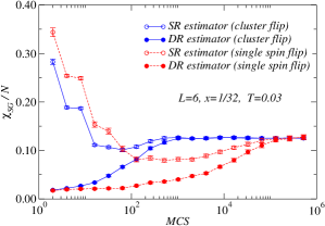
(a)

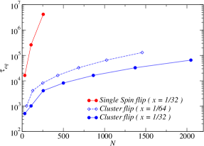
(b)

Figure 3: (a) Time variation of $\chi_{SG}/N$ calculated from both the double replica (DR) and the single replica (SR) estimators of the spin overlap function as defined in Eq. 7 using both the cluster algorithm (denoted by cluster flip) and the single spin flip algorithm (denoted by single spin flip) in combination with parallel tempering in temperature. The autocorrelation time $\tau_{eq}$ estimated from such an analysis is shown in (b) for various $N$ at $x=1/32$ and $x=1/64$.

Results: Using our improved cluster algorithm, we study the behavior of $\chi_{SG}$ (Eq. 5) and $\xi/L$ (Eq. 6) in the following ranges: $4\leq L\leq 16$ for $x=1/32$, $4\leq L\leq 20$ for $x=1/64$, and $6\leq L\leq 22$ for $x=1/128$ to understand the spin-glass transition at small $x$. The details regarding the simulation parameters are given in Appendix C. We check for the proper thermalization of these quantities by using a standard logarithmic binning analysis, where the different observables are calculated by using data only from the second half of the measurements, the second quarter of them, the second eighth of them and so on. Equilibration is reliably achieved when at least the last three bins agree within error bars. The behavior of $\chi_{SG}$ and $\xi/L$ as a function of $T$ for different linear dimensions $L$ is shown in Fig. 4(a) and Fig. 4(b) for $x=1/128$ which strongly suggests a transition to a spin-glass phase as the temperature is lowered.

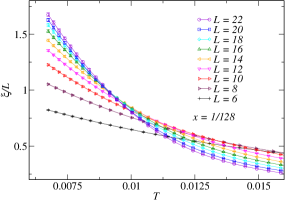
(a)

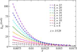
(b)

Figure 4: The behavior of (a) $\xi/L$ and (b) $\chi_{SG}$ as a function of $T$ shown for various $L$ at $x=1/128$.

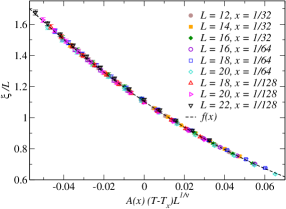
(a)

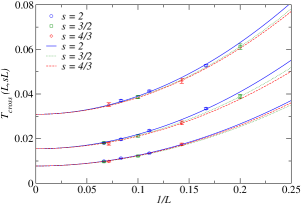
(b)

Figure 5: (a) Scaling collapse of $\xi/L$ assuming the form in Eq. 8(a). (b) Behaviour of the crossing point $T_{cross}(L,sL)$ as a function of $1/L$ and its fit to the form shown in Eq. 9.

To extract the transition temperature $T_{x}$ and establish the universality class of the transition, we now discuss the finite-size scaling behavior of these two quantities. Our results give strong evidence that the critical points at small $x$ are identical upto a simple $x$-dependent global rescaling and thus have the same universal physics. Assuming this scenario, to leading order in finite size scaling, $\xi/L$ and $\chi_{SG}$ behave as follows KatzgraberKY06 :

$$\xi/L =\mathcal{F}_{1}(A(x)(T-T_{x})L^{1/\nu})$$ (8a)

$$B(x)\chi_{SG} =L^{2-\eta}\mathcal{F}_{2}(A(x)(T-T_{x})L^{1/\nu})$$ (8b)

where $\mathcal{F}_{1,2}$ are universal functions, $\nu$ and $\eta$ are exponents characterizing the continuous transition, $T_{x}$ is the critical temperature at $x$ and $A(x),B(x)$ are “metric factors” that depend only on $x$.

We first perform the scaling collapse for $\xi/L$ since it has a smaller number of fitting parameters (Eq. 8(a)). We assume $T_{x}=ax(1+bx)$ to see the importance of the nonlinear terms at small $x$. The data collapse of $\xi/L$ (Fig. 5(a)) gives $a=1.10(2)$ and $b=0.62(15)$ which determines $T_{x}$ and the critical exponent $\nu=1.27(8)$ with a reduced chi square per degree of freedom $\bar{\chi}^{2}=1.14$ (see Eq. 10 for definition of $\bar{\chi}^{2}$). The metric factors are determined to be $A(x=1/64)=1.65(3)$ and $A(x=1/128)=2.77(6)$ keeping $A(x=1/32)=1$. Our estimate of $\nu$ agrees with that of Ref. AndresenKOS14, for uniaxial dipolar Ising spins in the dilute limit. For completeness, we show the data collapse of $\xi/L$ at each individual $x$ in Fig. 7(d), Fig. 7(e), Fig. 7(f) and give the extracted $T_{x},\nu$ and $\bar{\chi}^{2}$ in Table. 3.

We also perform a crossing point analysis of $\xi/L$ between systems of linear dimension $L$ and $sL$ (with a fixed $s$) at each $x$ to extract $T_{x}$. The crossing temperature, $T_{\mathrm{c}ross}(L,sL)$, should converge to $T_{x}$ as $L\rightarrow\infty$ in the following manner FernandezMGTY09 :

$$T_{\mathrm{c}ross}(L,sL)=T_{x}+A_{SG}(x,s)L^{-(1/\nu+\omega)}$$ (9)

where $A_{SG}(x,s)$ is a (non-universal) constant that depends on both $x$ and $s$ and $\omega$ is the exponent for the leading correction to scaling. Since Fig. 5(a) already shows strong evidence that the universality does not depend on $x$ (for small $x$), we therefore assume the combination $(1/\nu+\omega)$ to be independent of $x$ and use $s=2,3/2,4/3$ to obtain the crossing of $\xi/L$ curves for $(L,sL)$ for various $L$ at $x=1/32,1/64,1/128$. We then fit all the crossing point data for the different $x$ simultaneously to Eq. 9 by assuming $T_{x}\propto x$ and $A_{SG}(x,s)$ to be different constants depending on the values of $x$ and $s$ respectively. The result is shown in Fig. 5(b) and yields $T_{x}=1.00(3)x$ which is in good agreement with the previously obtained value of $T_{x}$ (Fig. 5(a)) from the scaling collapse of $\xi/L$. We also obtain $1/\nu+\omega=1.98(16)$ from the fit.

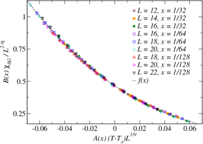
(a)

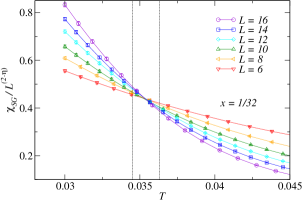
(b)

Figure 6: (a) Scaling collapse of the spin glass susceptibility $\chi_{SG}$ assuming the form in Eq. 8(b) after fixing $T_{x}$ and $\nu$ from the collapse of $\xi/L$. (b) The behavior of $\chi_{SG}/L^{2-\eta}$ versus $T$ shown for $\eta=0.22$ at $x=1/32$. The dotted vertical lines indicate $T_{x}\pm\Delta T_{x}$ where $T_{x}$ is extracted from the data collapse of $\xi/L$ and $\Delta T_{x}$ is the statistical error bar.

We now estimate the anomalous exponent $\eta$ from the behavior of $\chi_{SG}$. The exponent $\eta$ could not be reliably estimated for a dilute system of uniaxial dipolar Ising spins due to large finite-size corrections to scaling Gingras ; AndresenKOS14 . However, in the microscopic model adopted in this work (which provides a different lattice relization to the same universal physics), we can reliably extract $\eta$. The scaling collapse of $\chi_{SG}$ using Eq. 8(b) gives a large statistical error on the determination of $\eta=-0.35(69)$ when we keep $T_{x}(=ax(1+bx)),\nu,\eta,A(x),B(x)$ as free parameters for the fit. We, therefore, reduce the number of free parameters in the fit by fixing $T_{x}$ and $\nu$ from the previous data collapse of $\xi/L$. This gives us a much better estimate of $\eta=0.228(35)$ alongwith $A(x=1/64)=1.66(1),A(x=1/128)=2.69(3),B(x=1/64)=1.52(2),B(x=1/128)=2.24(4)$ (with $A(x=1/32)=B(x=1/32)=1$) with $\bar{\chi}^{2}=1.78$ (see data collapse of $\chi_{SG}$ in Fig. 6(a)). We note that the metric factor $A(x)$ obtained here coincides (within error bars) with that obtained from the fit of $\xi/L$ which is consistent with the expectation from Eq. 8. A further check for the obtained value of $\eta$ is provided by the behavior of $\chi_{SG}/L^{2-\eta}$ as a function of $T$ for various $L$ at a fixed $x$. A value of $\eta\approx 0.22$ gives a crossing point in $T$ in agreement with the estimate obtained from the data of $\xi/L$ (see Fig. 6(b) for the case of $x=1/128$). The finite size scaling procedure is summarized in Appendix D.

Conclusions: We have studied an emergent anisotropic dipolar system of Ising spins that arises when dipolar spin ice is weakly diluted with a fraction $x$ of non-magnetic impurities in the three-dimensional pyrochlore lattice. These emergent Ising spins have orientations that are neither random nor collinear but are picked according to the local easy axes of the occupied sites. This problem provides a lattice realization for studying the universal physics of a possible Ising spin glass transition in three dimensions, thus complementing the known cases of spin freezing for random dipoles, namely dense dipoles on a cubic lattice with random orientations denseglass , or dilute but collinear dipoles on a cubic lattice Gingras ; AndresenKOS14 .

Metropolis algorithm supplemented by parallel tempering in temperature is unable to equilibrate this problem except for a small number of dipoles because of the rapidly increasing autocorrelation time caused by rare-region effects of strongly interacting spin clusters. We use an improved cluster algorithm to relieve these equilibration bottlenecks and simulate much larger number of dipoles than possible using less elaborate algorithms.

Using finite-size scaling, we have been able to establish a finite temperature phase transition at small $x$. Furthermore, we present strong evidence that at small $x$, the universality class of the transition is independent of $x$ and estimate the critical exponents to be $\nu=1.27(8)$ and $\eta=0.228(35)$. The estimation of both the exponents $\nu$ and $\eta$ is a first for such dilute dipoles in three dimensions.

Our algorithm is also expected to give a significant speed-up for other Ising systems with atypical strong bonds, e.g., the recently introduced random Coulomb antiferromagnet in three dimensions RehnMY16 . Finally, beyond the thermodynamic phase transition, a detailed understanding of the nature of the dynamical slowdown and the resulting spatial heterogeneity in the local spin relaxation BiltmoH12 above the transition temperature $T_{x}$ for any local dynamics (Fig. 1(a), Fig. 1(b)) remains an interesting open problem ongoingwork .

Acknowledgements: We thank A. P. Young and Pushan Majumdar for several useful discussions. A.S. is partly supported through the Partner Group program between the Indian Association for the Cultivation of Science (IACS), Kolkata and the Max Planck Institute for the Physics of Complex Systems (MPIPKS), Dresden. The simulations were performed on the supercomputing clusters maintained by the Max Planck Computing and Data Facility (MPCDF). This work was in part supported by Deutsche Forchungsgemeinschaft (DFG) via grant SFB 1143 as well as Cluster of Excellence ct.qmat (EXC 2147, project id 39085490).

Appendix A Dependence of thermalization timescale on ($a_{s},b_{s},C_{L}$)

The cluster construction requires specification of three parameters $a_{s},b_{s}$ and $C_{L}$ as described in the main text. For most of the simulations reported in the paper, we take $a_{s}=1.3125$, $b_{s}=0.75$ and $C_{L}=N/5$ which is enough to make the last three bins agree for $\xi/L$ and $\chi_{SG}$ when performing logarithmic binning tests for equilibration. However, this is not true for the case of $L=22$ for the smallest dilution of $x=1/128$ that we considered (as can be seen from Fig. 7(a)). Here, we instead see that choosing $a_{s}=1.3125$, $b_{s}=47.25$ and $C_{L}=N/3$ and taking the probability of a cluster flip to be $50\%$ (instead of $15\%$) improves the equilibration significantly (Fig. 7(a)) and we use these parameters to also generate the data at $L=22,x=1/128$.

In our cluster construction procedure, the value of $\Delta J=b_{s}J_{s}$ scales linearly with $x$ if $a_{s}$ is kept fixed. As a result, unless $b_{s}$ is increased with decreasing $x$, the number of cluster sets increases for highly diluted systems at very low $x$. This is not ideal since (a) the different cluster sets are then not different enough and (b) with our considered probability distribution, the first few sets, i.e., $C_{0}$ and its neighboring sets are hardly chosen during the cluster flip. Thus, it is useful to increase $b_{s}$ as one goes to lower values of $x$. Furthermore, at low $x$, $T_{x}$ also decreases with $x$ and hence the size of the largest frozen cluster (with respect to single spin flips) is also bound to increase. We therefore increase $b_{s}$ significantly from $0.75$ to $47.25$ and $C_{L}$ from $N/5$ to $N/3$ for $L=22,x=1/128$. We also see that at low $x$, it is better to increase the relative probability of cluster flips with respect of single spin flips and therefore increase this from $15\%$ to $50\%$. The problem of optimizing over the parameters $a_{s}$, $b_{s}$ and $C_{L}$ has not been systematically addressed in this work and understanding this should lead to further significant speed-up at very low $x$ as Fig. 7(a) already demonstrates.

Appendix B Role of different cluster sets in equilibration

We explictly demonstrate the role of the different cluster sets in equilibrating the system by considering $N_{sample}=300$ independent disorder realizations for a system of size $L=10$ with $x=1/32$ at a rather low temperature of $T=0.015(\lesssim T_{x}/2)$ (Fig. 7(b) and Fig. 7(c)). The cluster sets are constructed for each disorder realization by taking the parameters to be $a_{s}=1.3125,b_{s}=0.75$ and $C_{L}=N/3$. The total number of cluster sets, $(n+1)$, is $5-6$ for most of the disorder realizations. We then create various cluster set combinations (given in Table 1) by either switching on the cluster sets one by one from $C_{n-4}$ to $C_{n}$ or from $C_{n}$ to $C_{n-4}$ (in the disorder realizations where $n>4$, the cluster sets $C_{n-5}$ and lower are not considered for this analysis). The parameters for the parallel tempering used are $T_{0}=0.015,c=0.065$ and $N_{T}=31$. We choose a local spin (cluster) flip with probability $85\%$ ($15\%$). The (relative) probability to choose a particular cluster set $C_{m}$ is then taken to be $P_{m}$ (see Table 1) according to the rule specified in the main text. We check the difference in thermalization time for the various cluster set combinations by performing a logarithmic binning analysis for $\xi/L$ and the results are displayed in Fig. 7(b) and Fig. 7(c).

It can be seen that neither $C_{n-4}$, $C_{n-4}$, $C_{n-3}$ nor $C_{n-4}$, $C_{n-3}$, $C_{n-2}$ satisfy the log binning thermalization test within the given number of MCS but their performance improves progressively. However, when the sets containing larger fraction of strong bonds are considered in $C_{n-4}$, $\cdots$, $C_{n-1}$ and $C_{n-4}$, $\cdots$, $C_{n}$, the system does equilibrate within the given number of MCS (Fig. 7(b)). What happens when we start switching on the clusters from $C_{n}$ to $C_{n-4}$? Here the effect is much more dramatic and already the cluster combination of $C_{n}$, $C_{n-1}$ equilibrates the system for the given number of MCS (note that the same is not true with just the cluster set $C_{n}$). The equilibration performance only improves slightly when we consider the combinations $C_{n}$, $C_{n-1}$, $C_{n-2}$, $C_{n}$, $\cdots$, $C_{n-3}$ and $C_{n}$, $\cdots$, $C_{n-4}$ (Fig. 7(c)). These results clearly show that it is important to attempt flipping clusters from the latter sets more frequently than to attempt flipping clusters from the earlier sets. In this manner, the average computational cost of $1$ MCS is also reduced as the larger clusters are flipped less often than the smaller clusters.

Cluster Combination	Relative Probabilities
$C_{n-4}$	1
$C_{n-4},C_{n-3}$	1/2,1/2
$C_{n-4},C_{n-3},C_{n-2}$	1/4,1/4,1/2
$C_{n-4},C_{n-3},C_{n-2},C_{n-1}$	1/8,1/8,1/4,1/2
$C_{n-4},C_{n-3},C_{n-2},C_{n-1},C_{n}$	1/16,1/16,1/8,1/4,1/2
$C_{n}$	1
$C_{n},C_{n-1}$	1/2,1/2
$C_{n},C_{n-1},C_{n-2}$	1/2,1/4,1/4
$C_{n},C_{n-1},C_{n-2},C_{n-3}$	1/2,1/4,1/8,1/8
$C_{n},C_{n-1},C_{n-2},C_{n-3},C_{n-4}$	1/2,1/4,1/8,1/16,1/16

Table 1: The relative probabilities to pick the individual cluster sets which have been used to generate the results of Fig. 4(a),(b)

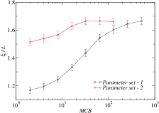
(a)

(b)

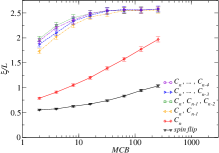
(c)

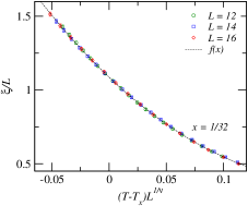
(d)

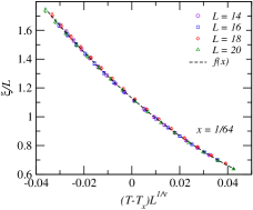
(e)

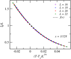
(f)

Figure 7: (a) Comparison of the logarithmic binning for $\xi/L$ for $L=22$ at $x=1/128$ using parameter set-1 ($a_{s}=1.3125,b_{s}=0.75,C_{L}=N/5$) and parameter set-2 ($a_{s}=1.3125,b_{s}=47.25,C_{L}=N/3$) with the local spin flip move chosen $85\%$ ($50\%$) in the former (latter) case. The disorder averaging is done over $N_{sample}=600$, and the parallel tempering parameters are $T_{0}=0.00675$, $c=0.031$ and $N_{T}=31$ (the result is shown for the lowest temperature $T_{0}$). Logarithmic binning thermalization test for $\xi/L$ for $L=10$, $x=1/32$ at a low temperature of $T=0.015(\lesssim T_{x}/2)$ where the cluster sets are switched on from $C_{n-4}$ to $C_{n}$ in (b) and from $C_{n}$ to $C_{n-4}$ in (c). The relative probabilities to pick the individual cluster sets is given in Table 1. In panels (a), (b), (c), one MCB equals 512 MC Sweeps in all the figures. The data collapse of $\xi/L$ at (d)$x=1/32$ (e) $x=1/64$ and (f) $x=1/128$. The extracted values of $T_{x}$ and $\nu$ are summarized in Table 3.

Appendix C Simulation parameters

Apart from $a_{s},b_{s},C_{L}$, the other simulation parameters that we need to specify are $T_{0}$, $c$ and $N_{T}$ to set up the parallel tempering protocol. We summarize the values of these parameters for different $L$ and $x$ and also $N_{MCS}$ (the number of MCS used), $N_{sample}$ used during the production runs in Table 2.

$x$	$L$	$T_{0}$	$c$	$N_{T}$	$N_{MCS}$	$N_{sample}$
1/32	4	0.03	0.20	15	$10\times 2^{19}$	2500
1/32	6	0.03	0.035	63	$10\times 2^{18}$	1500
1/32	8	0.03	0.035	63	$10\times 2^{17}$	1500
1/32	10	0.03	0.025	63	$10\times 2^{16}$	1500
1/32	12	0.03	0.025	63	$10\times 2^{17}$	1500
1/32	14	0.03	0.025	63	$10\times 2^{16}$	1500
1/32	16	0.03	0.030	31	$10\times 2^{17}$	1500
1/64	4	0.01	0.055	31	$10\times 2^{17}$	2100
1/64	6	0.01	0.055	31	$10\times 2^{17}$	2100
1/64	8	0.01	0.055	31	$10\times 2^{16}$	2100
1/64	10	0.01	0.040	31	$10\times 2^{17}$	1500
1/64	12	0.01	0.040	31	$10\times 2^{17}$	1500
1/64	14	0.0135	0.031	31	$10\times 2^{17}$	1500
1/64	16	0.0135	0.031	31	$10\times 2^{18}$	1500
1/64	18	0.0135	0.031	31	$10\times 2^{17}$	1500
1/64	20	0.0135	0.031	31	$10\times 2^{17}$	1500
1/128	6	0.00675	0.045	31	$10\times 2^{17}$	2500
1/128	8	0.00675	0.045	31	$10\times 2^{17}$	2500
1/128	10	0.00675	0.031	31	$10\times 2^{17}$	2500
1/128	12	0.00675	0.031	31	$10\times 2^{17}$	2500
1/128	14	0.00675	0.031	31	$10\times 2^{16}$	2200
1/128	16	0.00675	0.031	31	$10\times 2^{17}$	1500
1/128	18	0.00675	0.031	31	$10\times 2^{20}$	1500
1/128	20	0.00675	0.031	31	$10\times 2^{20}$	1500
1/128	22	0.00675	0.031	31	$10\times 2^{18}$	1500

Table 2: Parameters of the Monte Carlo simulations.

Appendix D Finite-size scaling

To estimate the $T_{x}$ and extract the critical exponents $\nu$ and $\eta$, we use the scaling forms given in Eq. 8 sufficiently close to the critical point. For $\xi/L$, we expand the scaling function $\mathcal{F}_{1}(X)$ (where $X=A(x)(T-T_{x})L^{1/\nu}$) as a third-order polynomial $\mathcal{F}_{1}(X)\equiv f(X)=a_{0}+a_{1}X+a_{2}X^{2}+a_{3}X^{3}$ and then perform a global fit to determine the unknown parameters $(a_{0},a_{1},a_{2},a_{3},a,b,\nu,A(x=1/64),A(x=1/128))$ [where $T_{x}=ax(1+bx)$ is assumed at small $x$ and the metric factor $A(x=1/32)=1$] by minimising the reduced chi square per degree of freedom $\bar{\chi}^{2}$ defined by

$$\bar{\chi}^{2}=\frac{1}{N_{d}-M}\sum_{i=1}^{N_{d}}(y_{i}-f(X_{i}))^{2}/\sigma_{i}^{2}$$ (10)

where $N_{d}$ equals the total number of data points, $M$ denotes the number of fitting parameters, $y_{i}$ denotes the mean value of the $i$-th data point, $\sigma_{i}$ denotes the error in the $i$-th data point and $f(X_{i})$ denotes the fitting function. The fits are considered of good quality when $\bar{\chi}^{2}\lessapprox 1$. Since all temperatures are simulated with the same disorder realization in the parallel tempering procedure, the fitted data is correlated. We therefore apply a bootstrap analysis to the data to estimate the statistical error bars on the various fit parameters. It is useful to emphasize here that the quoted error bars are only statistical errors since estimating systematic errors properly requires a reliable knowledge of the corrections due to scaling. For $\chi_{SG}$, we again use the scaling form given in Eq. 8(b) and expand the scaling function $\mathcal{F}_{2}$ as a third-order polynomial. We further fix the values of $a,b$ that determine $T_{x}=ax(1+bx)$ and the exponent $\nu$ from the previous fit of $\xi/L$ and then perform the minimization of $\bar{\chi}^{2}$ to determine the exponent $\eta$ and the other fitting parameters.

We show the data collapse of $\xi/L$ at each individual $x$ in Fig. 7(d), Fig. 7(e) and Fig. 7(f) for completeness. The extracted values of $T_{x}$ and $\nu$ are shown in Table 3 and is fully consistent with the scenario that $T_{x}\propto x$ and the universality of the critical point is independent of $x$ for small $x$.

$x$	$T_{x}$	$\nu$	$\bar{\chi}^{2}$
1/32	0.0351(8)	1.21(6)	0.73
1/64	0.0171(4)	1.30(7)	0.98
1/128	0.0090(2)	1.26(4)	1.06

Table 3: $T_{x}$, $\nu$ and $\bar{\chi}^{2}$ obtained from the data collapse of $\xi/L$ at $x=1/32$, $x=1/64$ and $x=1/128$ (see Fig. 7(d),(e),(f)).

References

- (1) V. Cannella and J. A. Mydosh, Magnetic Ordering in Gold-Iron Alloys, Phys. Rev. B 6, 4220 (1972).
- (2) M. A. Ruderman and C. Kittel, Indirect Exchange Coupling of Nuclear Magnetic Moments by Conduction Electrons, Phys. Rev. 96, 99 (1954); T. Kasuya, A Theory of Mettalic Ferro- and Antiferromagnetism on Zener’s Model, Progress of Theoretical Physics, 16, 45 (1956); K. Yoshida, Magnetic Properties of Cu-Mn Alloys, Phys. Rev. 106, 893 (1957).
- (3) K. Binder and A. P. Young, Spin glasses: Experimental facts, theoretical concepts, and open questions, Rev. Mod. Phys. 58, 801 (1986).
- (4) S. F. Edwards and P. W. Anderson, Theory of spin glasses, J. Phys. F 5, 965 (1975).
- (5) M. Baity-Jesi et al., Critical parameters of the three-dimensional Ising spin glass, Phys. Rev. B 88, 224416 (2013).
- (6) M. Hasenbusch, A. Pelissetto, and E. Vicari, Critical behavior of three-dimensional Ising spin models, Phys. Rev. B 78, 214205 (2008).
- (7) J. A. Mydosh, Spin Glasses: An Experimental Introduction, (Taylor & Francis, London 1993).
- (8) H. Kawamura, Dynamical Simulation of Spin-Glass and Chiral-Glass Orderings in Three-Dimensional Heisenberg Spin Glasses, Phys. Rev. Lett. 80, 5421 (1998).
- (9) K. Hukushima and H. Kawamura, Monte Carlo simulations of the phase transition of the three-dimensional isotropic Heisenberg spin glass, Phys. Rev. B 72, 144416 (2005).
- (10) L. W. Lee and A. P. Young, Large-scale Monte Carlo simulations of the isotropic three-dimensional Heisenberg spin glass, Phys. Rev. B 76, 024405 (2007).
- (11) L. A. Fernandez, V. Martin-Mayor, S. Perez-Gaviro, A. Tarancon, and A. P. Young, Phase transition in the three dimensional Heisenberg spin glass: Finite-size scaling analysis, Phys. Rev. B 80, 024422 (2009).
- (12) M. J. P. Gingras and P. Henelius, Collective phenomena in the LiHoxY1-xF4 quantum Ising magnet: Recent progress and open questions, J. Phys. Conf. Ser. 320, 012001 (2011).
- (13) D. H. Reich, B. Ellman, J. Yang, T. F.‘Rosenbaum, G. Aeppli, and D. P. Belanger, Dipolar magnets and glasses: Neutron-scattering, dynamical, and calorimetric studies of randomly distributed Ising spins, Phys. Rev. B 42, 4631 (1990).
- (14) J. A. Quilliam, S. Meng, C. G. A. Mugford, and J. B. Kycia, Evidence of spin glass dynamics in dilute LiHoxY1-xF4, Phys. Rev. Lett. 101, 187204 (2008).
- (15) M. J. Stephen and A. Aharony, Percolation with long-range interactions, J. Phys. C 14, 1665 (1981).
- (16) H.J. Xu, B. Bergresen, F. Niedermayer, and Z. Racz, Ordering of Ising Dipoles, J. Phys. Condens. Matter 3, 4999 (1991).
- (17) A. Biltmo and P. Henelius, Unreachable glass transition in dilute dipolar magnet, Nat. Commun. 3, 857 (2012).
- (18) G. Ayton, M. Gingras and G. Patey, Ferroelectric and dipolar glass phases of non crystalline systems, Phys. Rev. E 56, 562 (1997).
- (19) J. Snider and C. C. Yu, Absence of dipole glass transition for randomly dilute classical Ising dipoles, Phys. Rev. B 72, 214203 (2005).
- (20) A. Biltmo and P. Henelius, Low-temperature properties of the dilute dipolar magnet , Phys. Rev. B 78, 054437 (2008).
- (21) A. Biltmo and P. Henelius, Phase diagram of dilute magnet , Phys. Rev. B 76, 054423 (2007).
- (22) K.-M. Tam and M. J. P. Gingras, Spin-Glass Transition at Nonzero Temperature in a Disordered Dipolar Ising System: The Case of , Phys. Rev. Lett 103, 087202 (2009).
- (23) J. C. Andresen, H. G. Katzgraber, V. Oganesyan and M. Schechter, Existence of a Thermodynamic Spin-Glass Phase in the Zero-Concentration Limit of Anisotropic Dipolar Systems, Phys. Rev. X 4, 041016 (2014).
- (24) X. Ke, R. S. Freitas, B. G. Ueland, G. C. Lau, M. L. Dahlberg, R. J. Cava, R. Moessner, and P. Schiffer, Nonmonotonic Zero-Point Entropy in Diluted Spin ice, Phys. Rev. Lett. 99, 137203 (2007).
- (25) T. Lin, X. Ke, M. Thesberg, P. Schiffer, R. G. Melko, and M. J. P. Gingras, Nonmonotonic residual entropy in diluted spin ice: A comparison between Monte Carlo simulations of diluted dipolar spin ice models and experimental results, Phys. Rev. B 90, 214433 (2014).
- (26) C. Castelnovo, R. Moessner, and S. L. Sondhi, Spin ice, fractionalization, and topological order, Annu. Rev. Condens. Matter Phys. 3 35 (2012).
- (27) S. V. Isakov, K. Gregor, R. Moessner, and S. L. Sondhi, Dipolar Spin Correlations in Classical Pyrochlore Magnets, Phys. Rev. Lett. 93, 167204 (2004).
- (28) C. L. Henley, Power-law spin correlations in pyrochlore antiferromagnets, Phys. Rev. B 71, 014424 (2005).
- (29) A. Sen, R. Moessner, and S. L. Sondhi, Coulomb Phase Diagnostics as a Function of Temperature, Interaction Range, and Disorder, Phys. Rev. Lett. 110, 107202 (2013).
- (30) A. P. Ramirez, A. Hayashi, R. J. Cava, R. Siddharthan and B. S. Shastry, Zero-point entropy in ’spin ice’, Nature 399, 333 (1999).
- (31) C. Castelnovo, R. Moessner, and S. L. Sondhi, Magnetic monopoles in spin ice, Nature 451, 42 (2008).
- (32) A. Sen and R. Moessner, Topological spin glass in diluted spin ice, Phys. Rev. Lett. 114, 247207 (2015).
- (33) K. Janzen, A. K. Hartmann, and A. Engel, Replica Theory for Levy Spin Glasses, J. Stat. Mech. 2008, P04006.
- (34) J. C. Andresen, K. Janzen, and H. G. Katzgraber, Critical Behavior and Universality in Levy Spin Glasses, Phys. Rev. B 83, 174427 (2011).
- (35) R. H. Swendsen and J.-S. Wang, Nonuniversal critical dynamics in Monte Carlo simulations, Phys. Rev. Lett. 58, 86 (1987).
- (36) U. Wolff, Collective Monte Carlo Updating for Spin Systems, Phys. Rev. Lett. 62, 361 (1989).
- (37) S. T. Bramwell and M. J. P. Gingras, Spin ice state in frustrated magnetic pyrochlore materials, Science 294, 1495 (2001).
- (38) Z.Wang and C. Holm, Estimate of the Cutoff Errors in the Ewald Summation for Dipolar Systems, J. Chem. Phys. 115, 6351 (2001).
- (39) K. Hukushima and K. Nemoto, Exchange Monte Carlo Method and Applications to Spin Glass Simulations, J. Phys. Soc. Jpn. 65, 1604 (1996).
- (40) Placing a ghost spin on a site rules out any other on the neighboring six sites of the lattice (see Ref. SenM15 ), leading to a maximum .
- (41) A. T. Gabriel, T. Meyer, and G. Germano, Molecular Graphics of Convex Body Fluids, J. Chem. Theory Comput. 4, 468 (2008).
- (42) R. N. Bhatt and A. P. Young, Numerical studies of Ising spin glass in two, three and four dimensions, Phys. Rev. B 37, 5606 (1988).
- (43) H. G. Katzgraber, M. Körner, and A. P. Young, Universality in three-dimensional Ising spin glasses: A Monte Carlo study, Phys. Rev. B 73, 224432 (2006).
- (44) L. A. Fernandez, V. Martin-Mayor, S. Perez-Gaviro, A. Tarancon, and A. P. Young, Phase transition in the three dimensional Heisenberg spin glass: Finite-size scaling analysis, Phys. Rev. B 80, 024422 (2009).
- (45) J. F. Fernández, Monte Carlo study of the equilibrium spin-glass transition of magnetic dipoles with random anisotropy axes, Phys. Rev. B 78, 064404 (2008).
- (46) J. Rehn, R. Moessner, and A. P. Young, Spin glass behavior in a random Coulomb antiferromagnet, Phys. Rev. E 94, 032124 (2016).
- (47) T. K. Bose et al., work in progress.