COP: Customized Deep Model Compression via Regularized Correlation-Based Filter-Level Pruning

Abstract

Neural network compression empowers the effective yet unwieldy deep convolutional neural networks (CNN) to be deployed in resource-constrained scenarios. Most state-of-the-art approaches prune the model in filter-level according to the “importance” of filters. Despite their success, we notice they suffer from at least two of the following problems: 1) The redundancy among filters is not considered because the importance is evaluated independently. 2) Cross-layer filter comparison is unachievable since the importance is defined locally within each layer. Consequently, we must manually specify layer-wise pruning ratios. 3) They are prone to generate sub-optimal solutions because they neglect the inequality between reducing parameters and reducing computational cost. Reducing the same number of parameters in different positions in the network may reduce different computational cost. To address the above problems, we develop a novel algorithm named as COP (correlation-based pruning), which can detect the redundant filters efficiently. We enable the cross-layer filter comparison through global normalization. We add parameter-quantity and computational-cost regularization terms to the importance, which enables the users to customize the compression according to their preference (smaller or faster). Extensive experiments have shown COP outperforms the others significantly. The code is released at https://github.com/ZJULearning/COP.

1 Introduction

The growing demands of deploying deep models to resource-constrained devices such as mobile phones and FPGA have posed great challenges for us. Network pruning has become one of the most popular methods to compress the model without much loss in performance, and methods of network pruning could be divided into two categories: weight-level pruning Han et al. (2015); Guo et al. (2016); Dong et al. (2017) and filter-level pruning Li et al. (2016); Liu et al. (2017); He et al. (2018b).

The weight-level pruning methods try to find out unimportant weights and set them to zeros. In other words, weight-level pruning can compress deep models because it induces sparsity in filters. However, it contributes little to accelerating them unless specialized libraries (such as cuSPARSE) are used. Unfortunately, the support for these libraries on mobile devices, especially on FPGA is very limited. Thus, filter-level pruning methods are proposed to address this problem. They locate and remove unimportant filters in convolutional layers or unimportant nodes in fully connected layers. In this way, both space and inference time cost can be saved a lot.

Undoubtedly, the key factor influencing a filter-level pruning method’s performance is how it defines the importance of filters. We find the current state-of-the-art methods have at least two of the following problems.

High Redundancy.

Deep models with rich parameters may suffer from high redundancyDenil et al. (2013) among filters, i.e., different filters may have similar expressibility. Some methods (e.g., Li et al. (2016); Liu et al. (2017) only evaluate the importance based on the filter itself and neglect the correlations between filters.

Lack of Global Vision.

Under the approaches definition of some previous methods (e.g., Li et al. (2016); He et al. (2018b, a); Luo et al. (2017)), the filters can be only compared within the same layer. Thus, it is difficult to specify how many filters should be pruned for each layer.

Sub-optimal Pruning Strategy.

All the existing methods are prone to generate sub-optimal pruning strategies because they neglect that pruning the same number of parameters may not means reducing the same amount of computation cost. Take Figure LABEL:fig:vgg as an example. Pruning the same number of parameters in different layers of VGG16, we may reduce more computation cost by pruning the lower layers. Previous methods are insensitive to such differences.

To address the above limitations, we develop a correlation-based pruning algorithm (COP) to detect the redundancy among filters efficiently. We normalize the filter importance of different layers to the same scale to enable global comparison. In addition, we add parameter-quantity and computation-cost regularization terms to enable fine-grained filter pruning. The users can customize the compression simply through weight allocation according to their preference, i.e., whether they want to reduce more parameters or inference complexity.

It is worthwhile to highlight the advantages of COP:

• We propose a novel filter-level pruning algorithm for deep model compression, which can a) reduce the redundancy among filters significantly, b) learn proper pruning ratios for different layers automatically, and c) enable fine-grained pruning given users’ preference.

• Extensive experiments on public datasets have demonstrated COP’s advantages over the current state-of-the-art methods.

• We also evaluate COP on specially designed compact neural network, MobileNets. COP still produces reasonably good compression ratio with little loss on the inference performance.

2 Related Works

Network pruning has become one of the most popular methods to compress and accelerate deep CNNs. Network pruning includes two categories: weight-level pruning and filter-level pruning. Weight-level pruning sets unimportant weights in filters to zero, which induces sparsity into filters. However, according to Luo et al. (2017); Liu et al. (2017); Molchanov et al. (2016), it is difficult for weight-level pruning to accelerate deep CNNs without specialized libraries or hardware. Filter-level pruning solves this problem, it prunes unimportant filters in convolutional layers, which compresses and accelerates the deep CNNs simultaneously.

In recent years, many filter-level pruning methods have been proposed.  Li et al. (2016) evaluates the importance of filters through the sum of its absolute weights, i.e., $l1$ norm, and decide pruned ratio for each layer manually.  Luo et al. (2017) evaluates the importance of filters through reconstruction loss and use the same pruned ratio for all layers, i.e., large loss induced by pruning means high importance of the pruned filter.  He et al. (2017) evaluates the importance of filters based on LASSO regression. All the methods mentioned above only evaluate the local importance for filters, i.e., the importance could only be compared within the same layer, so they have to specify the pruned ratio for each layer manually.  Molchanov et al. (2016) evaluates the importance of filters through Taylor expansion, whose value could be compared globally.  Liu et al. (2017) also evaluates the global importance of filters based on the scale of batch normalization (BN) layer. However, as we say in Section 1, all these methods neglect the inequality between reducing parameters and reducing computational cost, the users cannot customize the pruned model for different purposes(smaller or faster).

PFA is a filter-level pruning method, which decides the pruned ratio for each layer by performing PCA on feature maps and evaluates the importance of filters by doing correlation analysis on feature maps. PFA is similar to our method because both PFA and COP use correlation to evaluating the importance of filters, however, there are three main differences between PFA and COP: 1) PFA is a data-driven method. It performs the correlation analysis on the activated feature maps, while COP performs correlation analysis on the filter weights. PFA needs all the training data when evaluating the importance of filters, which consumes more computing resources; however, COP only uses the trained model parameters when evaluating filters’ importance. 2) PFA is a two-stage pruning method, i.e., it needs to perform PCA first and then correlation analysis when pruning filters; COP only performs correlation analysis. 3) As we mentioned in Section 1, PFA is a sub-optimal pruning method; COP uses two regularization terms to generate fine-grained pruning plans, so users could customize their pruned model for different purposes.

3 Algorithm

3.1 Symbols and Annotations

Assuming there are $L$ layers in a deep model, let $P^{l}$ be the $l_{th}$ layer in the deep model, whose input is $X^{l}$, output is $Y^{l}$ and weight is $W^{l}$. We will omit superscript $l$ for simplicity in the cases of no confusion.

When $P^{l}$ is a fully connected layer, $W^{l}$ is of shape $M^{l}\times N^{l}$, where $M^{l}$ is the number of input nodes and $N^{l}$ is the number of output nodes; $X^{l}$ is of shape $M^{l}\times 1$; $Y^{l}$ is of shape $N^{l}\times 1$. Let $X^{l}_{m}$ be the $m_{th}$ node of $X^{l}$, $Y^{l}_{n}$ be the $n_{th}$ node of $Y^{l}$. Let $\vec{\omega}_{m}$ be the $m_{th}$ row of $W^{l}$, namely $\vec{\omega}_{m}=[W_{m,1},\cdots,W_{m,n}]$.

When $P^{l}$ is a convolutional layer, $W^{l}$ is of shape $K^{l}\times K^{l}\times M^{l}\times N^{l}$, where $K^{l}$ is the kernel width (assumed to be symmetric), $M^{l}$ is the number of input channel, $N^{l}$ is the number of output channel; $X^{l}$ is of shape $I^{l}\times I^{l}\times M^{l}$; $Y^{l}$ is of shape $O^{l}\times O^{l}\times N^{l}$; $I^{l}$, $O^{l}$ are the size of input and output feature maps respectively. $X^{l}_{m}$ is the $m_{th}$ input feature map in the $l_{th}$ layer. Let $\vec{\omega}_{i,j,m}$ be the vector $[W_{i,j,m,1},W_{i,j,m,2},\cdots,W_{i,j,m,n}]$.

$\mu_{\vec{\omega}_{m}}$ is the mean of $\vec{\omega}_{m}$. $\sigma_{\vec{\omega}_{m}}$ is the standard deviation of $\vec{\omega}_{m}$. Let $E[\cdot]$ be the expectation function.

Note that, in a convolutional layer, pruning feature maps is equivalent to pruning filters, and the importance of feature maps could also be seen as the importance of filters. Therefore, for simplicity, we will not differentiate pruning filters from pruning feature maps.

3.2 Overview

We propose three techniques to avoid the three limitations mentioned in Section 1. 1) Evaluate the correlation-based importance of filters to remove redundant filters. 2) Normalize the correlations from all layers to the same scale for global comparison. 3) Adding parameter-quantity and computational-cost regularization terms to the importance evaluation. The users could choose freely whether they want to reduce more parameters or more computational cost by adjusting the weights of two regularization terms.

3.3 Method

3.3.1 Normalized Correlation-Based Importance

We will first take fully connected layers as examples and introduce the calculation of correlation-based importance in detail, then generalize it to convolutional layers.

Figure LABEL:fig:fully is an illustration of our idea. In a fully connected layer, $Y_{n}$ is calculated as $Y_{n}=\sum_{m}W_{m,n}X_{m}$, we omit the bias term for simplicity. If $\exists m1,m2\in[1,M],\alpha\in\mathbb{R}$ such that $\vec{\omega}_{m2}\approx\alpha\vec{\omega}_{m1}$, then $Y_{n}$ could also be computed as Equation 1 for all $n\in[1,N]$. $\epsilon$ is the loss induced because $\vec{\omega}_{m2}$ and $\vec{\omega}_{m1}$ are not strictly linearly related. So, we could merge $X_{m1}$ and $X_{m2}$ through pruning and fine-tuning.

$$Y_{n}=\sum_{m\notin\{m1,m2\}}W_{m,n}X_{m}+W_{m1,n}X_{m1}+W_{m2,n}X_{m2}$$ (1)

$$=\sum_{m\notin\{m1,m2\}}W_{m,n}X_{m}+W_{m1,n}X_{m1}+\alpha W_{m1,n}X_{m2}+\epsilon$$

$$=\sum_{m\notin\{m1,m2\}}W_{m,n}X_{m}+W_{m1,n}(X_{m1}+\alpha X_{m2})+\epsilon$$

$\vec{\omega}_{m2}\approx\alpha\vec{\omega}_{m1}$ implies that $\vec{\omega}_{m1}$ and $\vec{\omega}_{m2}$ are activated in similar patterns. On the other hand, it also implies $X_{m1}$ and $X_{m2}$ express similar information. We propose to measure the redundancy between $\vec{\omega}_{m1}$ and $\vec{\omega}_{m2}$ by using Pearson correlation, which also indicates the similarity between $X_{m1}$ and $X_{m2}$ (Equation 2).

$$sim (X_{m1},X_{m2})=corr(\vec{\omega}_{m1},\vec{\omega}_{m2})$$ (2)

$$=\frac{E[(\vec{\omega}_{m1}-\mu_{\vec{\omega}_{m1}})(\vec{\omega}_{m2}-\mu_{\vec{\omega}_{m2}})]}{\sigma_{\vec{\omega}_{m1}}\sigma_{\vec{\omega}_{m2}}}$$

The redundancy evaluation mentioned above could be generalized to convolutional layer with slight modifications because a fully connected layer could be seen as a convolutional layer whose weights are of shape $1\times 1\times M\times N$. For a convolutional layer whose filters are of shape $K\times K\times M\times N$, one filter can be seen as a group of $K\times K$ independent nodes. We regroup the filter tensors into $K\times K$ sets of nodes and calculate the pair-wise node-correlations accordingly. Finally, we calculate the filter-correlation by averaging the node-correlations on the respective $K\times K$ nodes of the given filter (as shown in Equation 3).

$$sim(X_{m1},X_{m2})=\frac{1}{K^{2}}\sum_{i}^{K}\sum_{j}^{K}corr(\vec{\omega}_{i,j,m1},\vec{\omega}_{i,j,m2})$$ (3)

For two correlated filters, we have to remove one of them. It is hard to tell which is more important if we only look at their correlation. Instead, if one filter is highly correlated with many other filters, we believe it can be removed because other filters can take over its job. Thus, among the correlation coefficients between the given filter and the others, we select the $k$ highest ones and average them to get the importance of the filter.

However, the importance defined is still a local one because the correlations are calculated among filters within the same layer. Generally, the correlation distributions of different layers are quite different due to their different functions and scopes. Thus, we need to normalize the importance to enable cross-layer comparison. There are various methods to normalize the importance. Molchanov et al. (2016) proposed a simple layer-wise $l2$-normalization which re-scales the importance distributions of different layers. Similarly, one can also normalize different importance distributions with $l1$-normalization. However, we argue that they are not suitable for correlation-based importance because they will cause improper scaling of the importance. For instance, for layers with many filters, the importance of each filter tends to be very small because the denominator is large. Consequently, the procedure will always try to prune the layers with more filters. We propose to use $max$-normalization. Specifically, we normalize the correlation distribution of each layer by dividing them by the maximal importance to align the correlation distributions to $[0,1]$. Formally, we define the normalized importance as Equation 4.

$$\begin{split}Imp(X^{l}_{m})&=1-\frac{1}{k}\sum^{k}{TopK(\frac{sim(X^{l}_{m},X^{l}_{n})}{\max_{p\neq q}(sim(X^{l}_{p},X^{l}_{q}))})},\\ &p,q,n\in[1,M]\,and\,n\neq m\\ \end{split}$$ (4)

Dataset	Alg	Acc(%)	Prr(%)	Frr(%)
CIFAR10	VGG16	93.56	0.0	0.0
	NS∗	93.59	73.9	29.2
	PFA	93.16	87.3	60.9
	NRE	93.40	92.7	67.6
	SFP∗	92.99	73.0	73.0
	COP	93.31	92.8	73.5
	ResNet32	92.64	0.0	0.0
	NS∗	90.23	35.3	53.4
	SFP	92.08	39.2	41.04
	PFGM	91.93	52.7	53.2
	COP	91.97	57.5	53.9
CIFAR100	VGG16	72.59	0.0	0.0
	SFP∗	71.52	42.3	42.2
	PFA	71.19	66.9	42.9
	COP	71.77	73.2	43.1
	ResNet32	68.74	0.0	0.0
	SFP	67.83	33.8	33.9
	COP	68.29	35.2	34.2
ImageNet	VGG11	63.60	0.0	0.0
	NS	63.34	82.5	30.4
	COP	62.38	83.2	44.8
	ResNet18	70.29	0.0	0.0
	SFP	67.10	40.6	41.8
	PFGM	67.81	40.6	41.8
	COP	66.98	45.1	43.3

Table 1: The table shows the results of all the algorithms on CIFAR and ImageNet. Alg means the algorithm names. Acc means the classification accuracy, Prr means the parameter-reduction ratio, and Frr means the FLOPs-reduction ratio. Higher is better. VGG and ResNet are the baseline models for pruning. Results with “*” are got with their released code, and others are from original papers.

3.3.2 Regularizers

As we discussed above, reducing the same number of parameters from different positions in a neural network may reduce quite a different amount of computation cost. To make our approach aware of such differences, we add two regularization terms to enable fine-grained pruning plan generation. As a result, the users can customize the pruning plan through simple weight-allocation. Specifically, we add parameter-quantity and computational-cost regularization terms when evaluating the importance of filters. Pruning a filter of the $l_{th}$ layer influences the parameter quantity and computational cost of the $l_{th}$ layer and the $(l+1)_{th}$ layer, so the parameter quantity ($S^{l}$) and computational cost ($C^{l}$) related with the $l_{th}$ layer are defined in Equation 5. Further, the regularizers are defined in Equation 6. Note that filters in the same layer share the same regularizers, and regularizers for fully connected layers could be computed in a similar way. Adding these two terms to the importance defined above will empower the procedure with the sensitivity of parameter-quantity and computation-cost. Thus, it can generate fine-grained pruning plans.

$$S^{l} =(K^{l}K^{l}M^{l}N^{l})+(K^{l+1}K^{l+1}M^{l+1}N^{l+1})$$ (5)

$$C^{l} =2I^{l}I^{l}K^{l}K^{l}M^{l}N^{l}$$

$$+2I^{l+1}I^{l+1}K^{l+1}K^{l+1}M^{l+1}N^{l+1}$$

$$Reg^{l}= \beta(1-\frac{log{(C^{l})}}{log(max(C^{u}))})$$ (6)

$$+ \gamma(1-\frac{log({S^{l}})}{log(max(S^{u}))}),u\in[1,L]$$

Finally, we define the regularized importance of $X^{l}_{m}$ as Equation 7.

$$ReImp(X_{m}^{l})=Imp(X_{m}^{l})+Reg^{l}$$ (7)

The COP algorithm is a three-step pipeline : 1) Calculate the regularized importance for all filters and nodes; 2) Specify a global pruning ratio and remove the least important ones according to the ratio; 3) Fine-tune the pruned model with original data. Note that we only prune the network and fine-tune it once. In contrast, many existing methods follow an alternative-prune-and-fine-tune manner.

Dataset	Alg	Acc(%)	Prr(%)	Frr(%)
CIFAR10	Mob	93.90	0.0	0.0
	Mob-0.75	93.38	46.0	43.7
	Mob-0.50	92.64	74.4	74.0
	COP-0.50	93.39	67.2	59.5
	COP-0.30	92.67	83.2	75.6
ImageNet	Mob	66.09	0.0	0.0
	Mob-0.75	63.44	39.0	42.8
	Mob-0.50	58.17	63.7	73.8
	COP-0.70	64.52	42.9	47.0
	COP-0.40	58.39	74.1	79.0

Table 2: The table shows the results of pruning MobileNets on CIFAR10 and ImageNet. Mob means the baseline model. Mob-x means thinner MobileNet with width multiplier x. COP-x means the pruned MobileNets through our approach with filter-preserving ratio $x$.

Pruning for Depth-Separable Convolutional Layer.

A depth-separable convolutional layer contains a depth-wise convolutional layer and a point-wise convolutional layer. A point-wise convolutional layer is actually a convolutional layer whose filters are of shape $1\times 1\times M\times N$, so we prune the point-wise layers as normal convolutional layers. As for depth-wise convolutional layer, the number of input and output feature maps are always the same; the input feature maps of a point-wise layer are also the output feature maps of a depth-wise layer Howard et al. (2017). Therefore, pruning the point-wise layer will immediately prune the depth-wise layer; we do not need to prune the depth-wise layer again.

Pruning for Residual Block.

A residual block contains more than one convolutional layer, and the number of input and output feature maps must be equal for a residual block unless there is an extra linear projection in the block He et al. (2016). Thus for all residual blocks which do not contain a linear projection, we compute the mean importance of input and output feature maps as overall importance and prune them simultaneously. Please refer to Figure LABEL:fig:resnet for details.

4 Experimental Settings

Network	Algorithm	Acc(%)	Prr(%)	Frr(%)
VGG16	COPcos	93.11	73.0	72.6
	COPdp	92.27	71.9	71.1
	COPcor	93.31	92.8	73.5
	COPl2	63.60	92.2	66.5
	COPl1	92.98	92.5	66.7
	COPmax	93.31	92.8	73.5
ResNet32	COPcos	91.48	54.5	49.1
	COPdp	91.35	53.9	52.0
	COPcor	91.97	57.5	53.9
	COPl2	91.51	54.0	52.2
	COPl1	91.43	54.7	53.5
	COPmax	91.97	57.5	53.9

Table 3: The table shows the results of using different redundancy-detectors and global normalization methods in our model. “$cos$”, “$dp$”, “$cor$” mean cosine, dot-product and correlation redundancy detectors respectively, and “$l1$”, “$l2$” and “$max$” are global normalization methods. The experiments are performed on CIFAR10.

4.1 Datasets and Architecture

We perform the experiments on two well-known public datasets, CIFAR Krizhevsky and Hinton (2009) and ImageNet Russakovsky et al. (2015). Specifically, we use both CIFAR10 and CIFAR100 in the CIFAR collection.

We test the compression performance of different algorithms on several famous large CNN models, including VGGNet Simonyan and Zisserman (2014), ResNet He et al. (2016), and MobileNet Howard et al. (2017).

4.2 Evaluation Protocol

Following the previous works Jiang et al. (2018); Liu et al. (2017); Yu et al. (2018), we record the parameter-reduction ratio (Prr) and FLOPs-reduction ratio (Frr) of each algorithm compared with the original model. A higher parameter-reduction ratio means a smaller model size, and a higher FLOPs-reduction ratio means a faster inference.

4.3 Compared Algorithms

We select several recent state-of-the-art methods which are all filter-level pruning algorithms:

• NS Liu et al. (2017) evaluates the importance of filters according to the BN’s scaling factors .

• NRE Jiang et al. (2018) proposes to prune the model by minimizing the reconstruction error of nonlinear units.

• PFA Suau et al. (2018) decides the pruned ratio for each layer by performing PCA on feature maps. They evaluate the importance of filters by doing correlation analysis on feature maps.

• SFP He et al. (2018a) evaluates the importance of filters with $l2$-norm and prunes filters in a soft manner, i.e., the pruned filters may be retrieved after fine-tuning .

• PFGM He et al. (2018b) evaluates the importance of filters by analyzing the geometric correlation among the filters within the same layer.

We also compare our pruned MobileNets with thinner MobileNetsHoward et al. (2017). MobileNets are compact deep neural networks which reduce the models’ size and computational cost by replacing convolutional layers with depth-separable convolutional layers. Howard et al. (2017) also proposes thinner MobileNets to balance accuracy and resources consumption.

Algorithm	Acc(%)	Prr(%)	Frr(%)
VGG16	72.59	0.0	0.0
COP($\gamma=0$, $\beta=0$)	72.09	57.9	43.2
COP($\gamma=0$, $\beta=3$)	72.17	46.0	48.8
COP($\gamma=1$, $\beta=1$)	71.98	63.8	47.4
COP($\gamma=3$, $\beta=0$)	71.77	73.2	43.1
ResNet32	68.74	0.0	0.0
COP($\gamma=0$, $\beta=0$)	68.09	33.0	32.9
COP($\gamma=0$, $\beta=3$)	68.29	35.2	34.2
COP($\gamma=1$, $\beta=1$)	68.21	40.4	22.9
COP($\gamma=3$, $\beta=0$)	68.26	41.1	18.6

Table 4: The table shows the results of using different $\beta$ and $\gamma$ on CIFAR100. $\beta$ is the weight of computational-cost regularization terms, and $\gamma$ is the weight of parameter-quantity regularization terms.

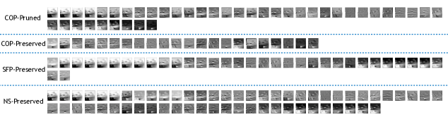
Figure 4: The figure shows the output feature maps of “conv1_1” in VGG16; the input is a random image from CIFAR10. COP-pruned means feature maps which are pruned by COP, COP-preserved means feature maps which are not pruned. SFP-preserved and NS-preserved mean feature maps which are preserved by these two algorithms. As the figure shows, COP-pruned contains many feature maps which look similar, but feature maps in COP-preserved are less similar to each other. However, SFP-preserved and NS-preserved still contain many feature maps which are similar, so the model pruned by these two algorithms are still of high redundancy. The figure implies that COP eliminates more redundancy of CNNs than SFP and NS.

4.4 Configuration

We set the batch-size of the stochastic gradient descent algorithm (SGD) to be 128, the momentum coefficient to be 0.9 for all models on CIFAR. For the VGG16 model on CIFAR, we use a weight decay rate of 0.0015, and we use a weight decay rate of 0.0006 and 0.0002 for the ResNet32 and MobileNet respectively on CIFAR.

When training on ImageNet dataset, we use the same architecture and training policy with the original paper Simonyan and Zisserman (2014) for VGG11. We use the same architecture with the original paper Howard et al. (2017) for MobileNets but the same training policy with VGG11 because it takes too much time to train MobileNets with the official training policy.

We use $k=3$ for $TopK$ when pruning the model.

5 Results and Analysis

5.1 Compression Efficiency

For the methods which do not report the results on given datasets and do not release their code either, we pass them in the experiments. The performance of different algorithms on the three datasets is given in Table 1, we experiment with several pruned ratio on COP and choose the maximal pruned ratio under the constraint of acceptable accuracy loss. On CIFAR, all the algorithms prune the VGG16 and ResNet32 models to get their compressed versions. On ImageNet, all the algorithms prune the VGG11 and ResNet18 models to get their compressed versions. As is shown in Table 1, we can draw some conclusions as follows:

1. COP achieves a higher compression ratio and speedup ratio with similar accuracy to other algorithms. Especially, COP gets the highest numbers on all three metrics on CIFAR100.

2. COP can prune much more parameters than most of the compared algorithms (e.g., NS, SFP, and PFGM) on different datasets and architecture because COP can detect the redundancy among filters better.

3. For the algorithms which can prune the similar number of parameters to COP (e.g., NRE and PFGM), COP gets more speed-up, which is the contribution of the computation-cost and parameter-size regularizers.

Though the MobileNet is a specially designed compact network, we can still prune it without much performance loss. The results are given in Table 2. MobileNet has its own way to compress itself Howard et al. (2017). We can see that COP can get better numbers in all the metrics.

5.2 Ablation Study

Redundancy Detector.

We have tried dot-product similarity, cosine similarity, and Pearson correlation as the redundancy detectors, and also tried $l1$-, $l2$-, and $max$-normalization methods as discussed above. The results are shown in Table 3. We can see that Pearson correlation and $max$-normalization are the best configurations because the Pearson correlation detect the redundancy better and the $max$-normalization is insensitive to the layer-width.

Regularizer Efficiency.

We try different weights for two regularization terms, and the results are shown in Table 4. We can see that the regularizer do have significant impacts on the compression. Larger $\gamma$ reduces more parameters while larger $\beta$ reduces more computation cost, which is exactly consistent with our expectation.

5.3 Case Study

COP focuses on observing redundant filters, so our pruned models contain less redundancy than others. With less redundancy, feature maps in the model mainly express diversified information. Figure 4 is an example of visualized feature maps of “conv1_1” in VGG16. Every feature map pruned by COP expresses similar information to those preserved. We compare COP with SFP and NS. SFP and NS can prune many unimportant feature maps, but there are still some similar feature maps being preserved.

6 Conclusion

We propose a novel filter-level pruning method, COP, to address the limitations of previous works in the following aspects: removing redundancy among filters; enabling cross-layer importance comparison; generating fine-grained pruning strategies (sensitive to desired computation cost and model size). Extensive experiments have shown our significant advantages over other state-of-the-art methods. Moreover, COP can also prune specially designed compact networks such as MobileNet and get larger compression ratio and speedup ratio than its own compression method.

References

- Denil et al. [2013] Misha Denil, Babak Shakibi, Laurent Dinh, Nando De Freitas, et al. Predicting parameters in deep learning. In Advances in Neural Information Processing Systems, pages 2148–2156, 2013.
- Dong et al. [2017] Xin Dong, Shangyu Chen, and Sinno Pan. Learning to prune deep neural networks via layer-wise optimal brain surgeon. In Advances in Neural Information Processing Systems, pages 4857–4867, 2017.
- Guo et al. [2016] Yiwen Guo, Anbang Yao, and Yurong Chen. Dynamic network surgery for efficient dnns. In Advances In Neural Information Processing Systems, pages 1379–1387, 2016.
- Han et al. [2015] Song Han, Huizi Mao, and William J Dally. Deep compression: Compressing deep neural networks with pruning, trained quantization and huffman coding. arXiv preprint arXiv:1510.00149, 2015.
- He et al. [2016] Kaiming He, Xiangyu Zhang, Shaoqing Ren, and Jian Sun. Identity mappings in deep residual networks. In European Conference on Computer Vision, pages 630–645. Springer, 2016.
- He et al. [2017] Yihui He, Xiangyu Zhang, and Jian Sun. Channel pruning for accelerating very deep neural networks. In International Conference on Computer Vision, volume 2, 2017.
- He et al. [2018a] Yang He, Guoliang Kang, Xuanyi Dong, Yanwei Fu, and Yi Yang. Soft filter pruning for accelerating deep convolutional neural networks. In International Joint Conference on Artificial Intelligence, pages 2234–2240. AAAI Press, 2018.
- He et al. [2018b] Yang He, Ping Liu, Ziwei Wang, and Yi Yang. Pruning filter via geometric median for deep convolutional neural networks acceleration. arXiv preprint arXiv:1811.00250, 2018.
- Howard et al. [2017] Andrew G Howard, Menglong Zhu, Bo Chen, Dmitry Kalenichenko, Weijun Wang, Tobias Weyand, Marco Andreetto, and Hartwig Adam. Mobilenets: Efficient convolutional neural networks for mobile vision applications. arXiv preprint arXiv:1704.04861, 2017.
- Jiang et al. [2018] Chunhui Jiang, Guiying Li, Chao Qian, and Ke Tang. Efficient dnn neuron pruning by minimizing layer-wise nonlinear reconstruction error. In International Joint Conference on Artificial Intelligence, volume 2018, pages 2–2, 2018.
- Krizhevsky and Hinton [2009] Alex Krizhevsky and Geoffrey Hinton. Learning multiple layers of features from tiny images. Technical report, Citeseer, 2009.
- Li et al. [2016] Hao Li, Asim Kadav, Igor Durdanovic, Hanan Samet, and Hans Peter Graf. Pruning filters for efficient convnets. arXiv preprint arXiv:1608.08710, 2016.
- Liu et al. [2017] Zhuang Liu, Jianguo Li, Zhiqiang Shen, Gao Huang, Shoumeng Yan, and Changshui Zhang. Learning efficient convolutional networks through network slimming. In IEEE International Conference on Computer Vision, pages 2755–2763. IEEE, 2017.
- Luo et al. [2017] Jian-Hao Luo, Jianxin Wu, and Weiyao Lin. Thinet: A filter level pruning method for deep neural network compression. In IEEE International Conference on Computer Vision, pages 5068–5076. IEEE, 2017.
- Molchanov et al. [2016] Pavlo Molchanov, Stephen Tyree, Tero Karras, Timo Aila, and Jan Kautz. Pruning convolutional neural networks for resource efficient inference. arXiv preprint arXiv:1611.06440, 2016.
- Russakovsky et al. [2015] Olga Russakovsky, Jia Deng, Hao Su, Jonathan Krause, Sanjeev Satheesh, Sean Ma, Zhiheng Huang, Andrej Karpathy, Aditya Khosla, Michael Bernstein, et al. Imagenet large scale visual recognition challenge. International Journal of Computer Vision, 115(3):211–252, 2015.
- Simonyan and Zisserman [2014] Karen Simonyan and Andrew Zisserman. Very deep convolutional networks for large-scale image recognition. arXiv preprint arXiv:1409.1556, 2014.
- Suau et al. [2018] Xavier Suau, Luca Zappella, and Nicholas Apostoloff. Network compression using correlation analysis of layer responses. arXiv preprint arXiv:1807.10585, 2018.
- Yu et al. [2018] Ruichi Yu, Ang Li, Chun-Fu Chen, Jui-Hsin Lai, Vlad I Morariu, Xintong Han, Mingfei Gao, Ching-Yung Lin, and Larry S Davis. Nisp: Pruning networks using neuron importance score propagation. In IEEE Conference on Computer Vision and Pattern Recognition, pages 9194–9203, 2018.