Aspects of Nosé and Nosé-Hoover Dynamics Elucidated

Abstract

Some paradoxical aspects of the Nosé and Nosé-Hoover dynamics of 1984 and Dettmann’s dynamics of 1996 are elucidated. Phase-space descriptions of thermostated harmonic oscillator dynamics can be simultaneously expanding, incompressible, or contracting, as is described here by a variety of three- and four-dimensional phase-space models. These findings illustrate some surprising consequences when Liouville’s continuity equation is applied to Hamiltonian flows.

I Introduction to Harmonic Oscillator Models

In 1984 Shuichi Nosé noticed that introducing a scale factor $s$ into the momenta made it possible to convert Gibbs’ microcanonical distribution to the canonical oneb1 ; b2 provided that [ 1 ] the “time-scaling factor” $s$ was governed by a temperature-dependent logarithmic potential and [ 2 ] the equations of motion ( assumed ergodic ) for the coordinates $\{\ q\ \}$ and momenta $\{\ p\ \}$ were multiplied by $s$. In principle and in practice this development made it possible to generate a dynamics consistent with the canonical ensemble, for systems small and large. And for ergodic systems such a dynamics, with the weights of dynamical states given by the Boltzmann factor $f(q,p)\propto e^{-{\cal H}/kT}$, can closely approximate the predictions of Gibbs’ canonical ensemble.

Hoover soon pointed out that the time-scaling factor $s$ was completely extraneous. He showed that the very same isothermal equations of motion could be derived directly from the phase space continuity equation,

$$(\dot{f}/f)=-(\dot{\otimes}/\otimes)\equiv-\sum[\ (\partial\dot{q}/\partial q)+(\partial\dot{p}/\partial p)\ ]$$

without introducing time scalingb3 ; b4 . Here $f$ is probability density and $\otimes$ represents an infinitesimal comoving phase volume. In Hoover’s adaptation of Nosé’s approach,“Nosé-Hoover dynamics”, the momentum conjugate to $s$ appears as a friction coefficient $\zeta$. $\zeta$ controls the dynamics via integral feedback using a target value of the kinetic temperature $mkT\equiv\langle\ p^{2}\ \rangle$. Here $k$ is Boltzmann’s constant and $m$ is a particle’s mass. Hoover found that the oscillator was far from ergodic. With Posch and Vesely he demonstrated the presence of a modest chaotic sea ( six percent of the stationary solution ) for the oscillator in addition to the preponderant ( 94% ) quasiperiodic toroidal solutionsb4 ; b5 . For the oscillator Nosé’s Hamiltonian ( with $\zeta=p_{s}$ ) is :

$${\cal H}_{Nos\acute{e}}=[\ q^{2}+(p/s)^{2}+\ln(s^{2})+\zeta^{2}\ ]/2\ .$$

For simplicity we choose $m$, $k$, and the oscillator force constant all equal to unity.

In 1996 Carl Dettmann showed that the Nosé-Hoover equations of motion can be derived from a scaled Hamiltonian, provided that the energy itself is set equal to zerob6 ; b7 .

$${\cal H}_{Dettmann}\equiv s{\cal H}_{Nos\acute{e}}\equiv 0\ .$$

These novel and surprising ideas are most easily displayed, illustrated, and understood by applying them again to the simplest possible problem, a one-dimensional harmonic oscillatorb3 ; b4 . Despite its lack of ergodicity such an oscillator provides a surprising source of topological variety, including intricately knotted phase-space trajectories ! Thus it has captured the attention of mathematicians as well as physicists and chemistsb8 ; b9 ; b10 ; b11 ; b12 ; b13 .

Our purpose here is entirely pedagogical. We focus on some surprising qualitative differences among the three- and four-dimensional flows described by Nosé, Dettmann, and Nosé-Hoover dynamics. Each of them can be analyzed in a four-dimensional $(q,p,s,\zeta)$ phase space, or in a three-dimensional subspace corresponding to the restriction of constant energy. Liouville’s Theorem, that Hamiltonian flows are incompressible, is a straightforward consequence of the motion equations :

$$\{\ \dot{q}=(\partial{\cal H}/\partial p)\ ;\ \dot{p}+-(\partial{\cal H}/\partial q)\ \}\longrightarrow\dot{f}=(\partial f/\partial t)+\sum\dot{q}(\partial f/\partial q)+\dot{p}(\partial f/\partial p)\equiv 0\ .$$

The Nosé ($s^{0}$) and Dettmann ($s^{1}$) oscillator Hamiltonians differ by just a factor $s$ :

$${\cal H}_{N,D}=(s^{0,1}/2)[\ q^{2}+(p/s)^{2}+\ln(s^{2})+\zeta^{2}\ ]\equiv 0\ ;\ \zeta\equiv p_{s}\ .$$

In both cases the resulting constant-energy dynamics develop in a three-dimensional constrained phase space. For instance we can choose a space described by the coordinate $q$, scaled momentum $(p/s)$, and friction coefficient $\zeta$. With the energy fixed any one of the four variables $(q,p,s,\zeta)$ can be determined from a convenient form of the constraint conditions :

$$s=e^{-(1/2)[\ q^{2}+(p/s)^{2}+\zeta^{2}\ ]}\ .$$

It is convenient to specify $(q,p/s,\zeta)$ and then to select $s$ to satisfy the ${\cal H}\equiv 0$ constraints. A consequence of the Dettmann multiplier $s^{1}$ is the simple relationship linking solutions of the Nosé and Dettmann Hamiltonians :

$$(\dot{q},\textstyle{\frac{d}{dt}}(p/s),\dot{\zeta})_{Dettmann}\equiv s(\dot{q},\textstyle{\frac{d}{dt}}(p/s),\dot{\zeta})_{Nos\acute{e}}\ .$$

The Nosé and Dettmann trajectories are identical in shape but are traveled at different speeds.

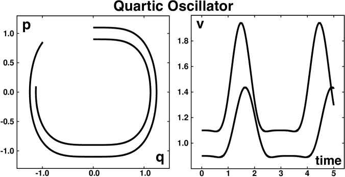
Figure 1: To the left we see two quartic oscillator trajectories in the $(q,p)$ phase space. The initial states are $(0,0.9)$ and $(0,1.1)$. The trajectories include 5000 fourth-order Runge-Kutta timesteps with $dt=0.001$. The Hamiltonian is ${\cal H}=(q^{4}/4)+(p^{2}/2)$. Because frequency increases with energy a constant comoving area shears as time progresses. Although both $f(q,p,t)$ and $\otimes(q,p,t)$ are constants of the motion, obeying Liouville’s Theorem, the phase-space speed, $\sqrt{\dot{q}^{2}+\dot{p}^{2}}=\sqrt{p^{2}+q^{6}}$ is far from constant, as is shown to the right in the Figure for the two trajectories..

It is tempting to think that the time spent in the volume element $dqd(p/s)d\zeta$ in the Dettmann case is proportional to $(1/s)\equiv e^{+(q^{2}+(p/s)^{2}+\zeta^{2})/2}$ compared to the Nosé case. But this relative probability of $e^{+{\cal H}/kT}$ is the reciprocal of what we would ( naively ) expect. Evidently the time argument is false. To see why, consider the Hamiltonian motion of a quartic oscillator with ${\cal H}=(p^{/}2)+(q^{4}/4)$ . Both the phase-space trajectory and the phase-space speed, $\sqrt{\dot{q}^{2}+\dot{p}^{2}}$ are shown in Figure 1. Though the Hamiltonian is constant, the speed in phase space, $\sqrt{q^{6}+p^{2}}$ varies. Liouville’s Theorem correctly shows that the probability density $f$ and the comoving area $\otimes$ are both constants along a trajectory. But, because the shape of the area varies with time there is no simple link between speed and $f$ or $\otimes$. It is the changing width of a comoving element perpendicular to the trajectory that destroys the supposed connection between speed and probability.

Our goal here is simply to point out this complex relationship between speed and probability in the simplest possible example. The difference can be even more dramatic in three- and four-dimensional problems. Let us look at the simplest such example problem in order to enrich our understanding. Consider the smallest periodic orbit traced out by the Dettmann, Nosé, and Nosé-Hoover equations of motion. We choose to begin the orbit with a higher kinetic energy, $1.55^{2}/2$, than the target value of $1/2$. With the initial conditions $(q,p/s,\zeta)=(0,1.55,0)$ we find $s=\sqrt{e^{-1.55^{2}}}=0.30082\rightarrow p=0.46627$ so that the initial condition $(q,p,s,\zeta)=(0,0.46627,0.30082,0)\rightarrow{\cal H}=0$.

II An expanding model in four dimensions

Nosé’s Hamiltonian, ${\cal H}_{N}=(1/2)[\ q^{2}+(p/s)^{2}+\ln(s^{2})+\zeta^{2}\ ]$, followed by time-scaling, leads to four equations of motion in $(q,p,s,\zeta)$ space:

$$\{\ \dot{q}=p/s\ ;\ \dot{p}=-sq\ ;\ \dot{s}=s\zeta\ ;\ \dot{\zeta}=[\ (p/s)^{2}-1\ ]\ \}\ \rightarrow(\partial\dot{s}/\partial s)=+\zeta\ .$$

Exactly these same motion equations follow more simply from Dettmann’s Hamiltonian, with no need of time scaling. Because our initial condition has a higher “temperature” $\langle\ (p/s)^{2}\ \rangle$ than the target of unity, the short-time friction coefficient $\zeta$ becomes positive, suggesting, from $\dot{s}=s\zeta$ that Nosé’s (or Dettmann’s ) oscillator’s phase volume begins by expanding rather than contracting. This expansion with a positive friction seems counter to Liouville’s Theorem, suggesting a paradox. Figure 2 shows the details of this four-dimensional problem. The time scaling factor $s$ is precisely equal to Gibbs’ canonical probability density. With the short-time positive friction, $\zeta>0$, the flow does contract rather than expand. Let us investigate this intriguing problem further.

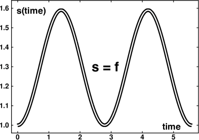
Figure 2: The time variation of two expressions for the probability density $f$ as measured once around a periodic orbit generated with Dettmann’s (or Nosé’s, with time scaling) Hamiltonian in the four-dimensional $(q,p,s,\zeta)$ phase space. The initial conditions are (0, 0.46627, 0.30082, 0) so that initially the scaled momentum is $(p/s)=1.55$ and the Hamiltonian vanishes. The thicker line is Gibbs’ canonical-ensemble density $e^{-[\ q^{2}+(p/s)^{2}+\zeta^{2}-1.55^{2}\ ]/2}$. The thinner white line overlaying the thicker black one shows the progress of the “time-scaling factor” $s(t)/s(0)=e^{\int_{0}^{t}\zeta(t^{\prime})dt^{\prime}}$. The perfect agreement demonstrates that the phase-space density $f(q,p,\zeta)$ can be obtained by measuring the phase-space compression ( but not the speed ) along the four-dimensional Hamiltonian trajectory with Dettmann’s constraint, ${\cal H}_{D}\equiv 0$ . But the early-time association of increasing phase volume, expected from $(\partial\dot{s}/\partial s)=\zeta>0$, is indeed paradoxical.

III An incompressible model ?

Dettmann’s Hamiltonian, ${\cal H}_{D}=(s/2)[\ q^{2}+(p/s)^{2}+\ln(s^{2})+\zeta^{2}\ ]$, with the constraint ${\cal H}_{D}\equiv 0$ imposed in the initial conditions, is not really incompressible :

$$\{\ \dot{q}=p/s\ ;\ \dot{p}=-sq\ ;\ \dot{s}=s\zeta\ ;\ \dot{\zeta}=-(1/2)[\ q^{2}-(p/s)^{2}+\ln(s^{2})+\zeta^{2}\ ]-1\ \}\ \rightarrow$$

$$(\partial\dot{s}/\partial s)+(\partial\dot{\zeta}/\partial\zeta)=+\zeta-\zeta=0\ [\ {\rm Incompressible?}\ ]\ .$$

The flow equations certainly maintain a comoving four-dimensional hypervolume unchanged in size. This is nothing more than the usual application of Liouville’s Theorem and is no surprise. But taking the zero energy constraint into account reduces the flow to three phase-space dimensions, as in the Nosé-Hoover picture. Let us look at that picture next. The quantitative details of the evolving phase probability are shown in Figure 3.

IV A contracting model in three dimensions

Here either Nosé-Hoover dynamics or a three-dimensional version of Dettmann’s Hamiltonian, including the constant-energy constraint, gives the same results. A time-reversible frictional force, $-\zeta p$, provides a steady-state Gaussian phase-space distribution $e^{-[\ q^{2}+p^{2}+\zeta^{2}\ ]/2}$ . In the two versions of dynamics the friction coefficient $\zeta$ is determined by integral feedback :

$$\{\ \dot{q}=p\ ;\ \dot{p}=-q-\zeta p\ ;\ \dot{\zeta}=p^{2}-1\ \}\ \longrightarrow(\partial\dot{p}/\partial p)=-\zeta\ .$$

Dettmann’s motion equations are identical to these if his scaled momentum $(p/s)$ is replaced by the symbol $p$. Here, with the relatively “hot” initial condition, the three-dimensional phase-space volume shrinks (correctly) initially due to contraction parallel to the momentum axis. So, for the three phase-space descriptions of the same physical problem we have found expansion, incompressibility, and compression, all for exactly the same phase-space states. We put these three examples forward from the standpoint of pedagogy, as a useful and memorable introduction to the significance of Liouville’s Theorem for isoenergetic flows. The constraint of constant energy can lead to qualitative differences in the evolution of $f$ and $\otimes$.

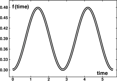
Figure 3: Two probability densities as measured once around a periodic Nosé-Hoover orbit in three-dimensional $(q,p,\zeta)$ space. The initial values are $(q,p,\zeta)=(0,1.55,0)$. The thicker line is Gibbs’ canonical $e^{-(q^{2}+p^{2}+\zeta^{2})/2}$. The overlaying thinner white line is $e^{\int_{0}^{t}\zeta(t^{\prime})dt^{\prime}}e^{-1.55^{2}/2}$. Here the perfect agreement shows that the integrated three-dimensional phase-space compression corresponds precisely to Gibbs’ canonical distribution.

V Acknowledgements

Over 35 years we have studied the paradoxical aspects of Shuichi Nosé’s pioneering contribution to statistical mechanics and nonlinear dynamics. During this time we have benefitted from the insights of dozens of colleagues throughout the world, most recently from Puneet Patra, Clint Sprott, Lei Wang, and Xiao-Song Yang, but dating back to Nosé himself plus Harald Posch and Franz Vesely. We thank them all.

References

- (1) S. Nosé, “A Unified Formulation of the Constant Temperature Molecular Dynamics Methods”, The Journal of Chemical Physics 81, 511-519 (1984).
- (2) S. Nosé, “A Molecular Dynamics Method for Simulations in the Canonical Ensemble”, Molecular Physics 52, 255-268 (1984).
- (3) W. G. Hoover, “Canonical Dynamics. Equilibrium Phase-Space Distributions”, Physical Review A 31, 1695-1697 (1985).
- (4) H. A. Posch, W. G. Hoover, and F. J. Vesely, “Canonical Dynamics of the Nosé Oscillator: Stability, Order, and Chaos”, Physical Review A 33, 4253-4265 (1986).
- (5) P. K. Patra, W. G. Hoover, C. G. Hoover, and J. C. Sprott, “The Equivalence of Dissipation from Gibbs’ Entropy Production with Phase-Volume Loss in Ergodic Heat-Conducting Oscillators”, International Journal of Bifurcation and Chaos 26, 1650089 (2016).
- (6) W. G. Hoover, “Mécanique de Nonéquilibre à la Californienne”, Physica A 240, 1-11 (1997).
- (7) C. P. Dettmann and G. P. Morriss, “Hamiltonian Reformulation and Pairing of Lyapunov Exponents for Nosé-Hoover Dynamics”, Physical Review E 55, 3693-3696 (1997).
- (8) J. C. Sprott, “Some Simple Chaotic Flows”, Physical Review E, 50, 647-650 (1994)
- (9) W. G. Hoover, “Remark on ‘Some Simple Chaotic Flows”’, Physical Review E, 51, 759-760 (1995).
- (10) L. Wang and X. S. Yang, “The Coexistence of Invariant Tori and Topological Horseshoes in a Generalized Nosé-Hoover Oscillator”, International Journal of Bifurcation and Chaos 27, 1750111 (2017).
- (11) L. Wang and X. S. Yang, “Global Analysis of a Generalized Nosé-Hoover Oscillator”, Journal of Mathematical Analysis and Applications 464, 370-379 (2018).
- (12) X. S. Yang, “Qualitative Analysis of the Nosé-Hoover Oscillator”, Qualitative Theory of Dynamical Systems (submitted, 2019).
- (13) W. G. Hoover, J. C. Sprott, and C. G. Hoover, “The Nosé-Hoover, Dettmann, and Hoover-Holian Oscillators”, arXiv 1906.03107, Prepared for the Qualitative Theory of Dynamical Systems (2019).