Rapid Particle Acceleration due to Recollimation Shocks and Turbulent Magnetic Fields in Injected Jets with Helical Magnetic Fields

Abstract

One of the key questions in the study of relativistic jets is how magnetic reconnection occurs and whether it can effectively accelerate blackelectrons in the jet. blackWe performed 3D particle-in-cell (PIC) simulations of a relativistic electron-proton jet of relatively large radius that carries a helical magnetic field. We focussed our investigation on the interaction between the jet and the ambient plasma and explore how the helical magnetic field affects the excitation of kinetic instabilities such as the Weibel instability (WI), the kinetic Kelvin-Helmholtz instability (kKHI), and the mushroom instability (MI). In our simulations these kinetic instabilities are indeed excited, and particles are accelerated. blackAt the linear stage we observe recollimation shocks near the center of the jet. As the electron-proton jet evolves blackinto the deep nonlinear stage, the helical magnetic field becomes untangled due to reconnection-like phenomena, and electrons are blackrepeatedly accelerated as they encounter magnetic-reconnection events in the turbulent magnetic field.

1 Introduction

Magnetic reconnection is ubiquitous in solar and magnetospheric plasmas, and it has been proposed that it is also an important mechanism for particle acceleration in Active Galactic Nuclei (AGN) and gamma-ray burst jets (Drenkhahn & Spruit, 2002; de Gouveia Dal Pino & Lazarian, 2005; de Gouveia Dal Pino et al., 2010; Uzdensky, 2011; Granot et al., 2011; Granot, 2012; McKinney & Uzdensky, 2012; Zhang & Yan, 2011; Giannios et al., 2009; Giannios, 2010, 2011; Komissarov, 2012; Sironi et al., 2015; de Gouveia Dal Pino et al., 2018; Kadowaki et al., 2018, 2019; Christie et al., 2019; Fowler et al., 2019). To study the fundamental physics of magnetic reconnection, numerous particle-in-cell (PIC) simulations have been performed that use the Harris model in a slab geometry (e.g., Daughton, 2011; Wendel et al., 2013; Karimabadi et al., 2014; Zenitani & Hoshino, 2005, 2008; Zenitani et al., 2011, 2013; Oka et al., 2008; Fujjimoto, 2011; Kagan et al., 2013; Sironi & Spitkovsky, 2011, 2014; Guo et al., 2015, 2016a, 2016b). Generally, studies in the slab configuration blackshow significant particle acceleration. However, this configuration blackdoes not apply to astrophysical jets, since the magnetic field appears to have a helical morphology close to the jet collimation/launching point (e.g., Tchekhovskoy, 2015; Hawley et al., 2015; Gabuzda, 2019).

blackIn jets MHD instabilities such as blackKelvin-Helmholtz (KHI) and blackthe kink instability (KI) can operate (e.g., Birkinshaw, 1984, 1996; Stone & Norman, 1994; Stone & Hardee, 2000). Recently, these MHD instabilities have been revisited using PIC simulations including kinetic processes (e.g., Sironi et al., 2013; Alves et al., 2015; Ardaneh et al., 2016; Nishikawa et al., 2019).

The interaction of relativistic jets with the plasma environment generates relativistic shocks that are mediated by the Weibel instability (WI) and accelerate particles. blackAt the velocity-shear boundary between the jet and the ambient medium magnetic turbulence is generated by the kinetic Kelvin-Helmholtz (kKHI) and the mushroom (MI) instability. blackRecent PIC simulations explored the WI, kKHI and MI in slab models of jets and later focussed on the evolution of cylindrical jets in helical magnetic-field geometry (e.g., Sironi et al., 2013; Alves et al., 2015; Ardaneh et al., 2016; Nishikawa et al., 2019). To achieve a complete understanding of the physics within the jet, global three-dimensional (3D) modeling blackneeds to be performed that enables investigation of the combined shock/shear blacklayer processes and includes kinetic effects. Our first PIC simulations of global jets were performed for unmagnetized plasmas (Nishikawa et al., 2016a). With this work we extend these studies to jets containing helical magnetic field.

One of the key questions we want to answer is how the helical magnetic field affects the growth of the kKHI, MI, and WI, and how and where in the jet structure particles are accelerated. In the latter respect, blackwe are particular interested in magnetic reconnection and its ability to aid in the rapid merging and breaking of the helical magnetic field carried by relativistic jets. Relativistic magnetohydrodynamic (RMHD) simulations demonstrate that jets with helical field develop kink instabilities (KI) (e.g., Mizuno et al., 2014; Singh et al., 2016; Barniol Duran et al., 2017; de Gouveia Dal Pino et al., 2018; Kadowaki et al., 2018, 2019); similar structures were found in PIC simulations (see, e.g., Nishikawa et al., 2019). It should be noted that MHD instabilities such as KHI and KI in jets have been investigated extensively (e.g., Birkinshaw, 1984; Stone & Norman, 1994; Stone & Hardee, 2000; Hawley et al., 2015). PIC simulations of a single flux rope modeling the jet that undergoes internal KI showed signatures of secondary magnetic reconnection (Markidis et al., 2014).

Recently, it was demonstrated that the development of the KI in relativistic strongly magnetized jets with helical magnetic field leads to the formation of highly tangled magnetic field and a large-scale inductive electric field promoting the rapid energization of particles through curvature drift acceleration (Alves et al., 2018, 2019). As initial condition these simulations assumed helical magnetic field in the jet frame supported by blackcounter-streaming electrons and positrons (ions). blackThere is neither velocity shear nor a jet head in their simulation, and so no velocity-shear instability such as kKHI and MI can be excited.

In this work we present results of our new study of relativistic jets containing helical magnetic field, which exhibit the nonlinear evolution of kinetic instabilities, magnetic reconnection, and the associated particle acceleration. We focus on electron-scale phenomena and set the jet size sufficient to accommodate the relevant electron kinetic instabilities that are not included in MHD simulations. The kinetic instabilities grow to the nonlinear stage, which is demonstrated by the disappearance of the helical magnetic field. Although our simulation results are insufficient to model the large-scale plasma flows of macroscopic parsec-scale jets, they explore relevant kinetic-scale physics within relativistic jet plasma.

2 PIC Simulation Setup of a Jet with Helical Magnetic Field Structure

In our simulations a cylindrical jet containing helical magnetic field blackand propagating in the $x$-direction is injected into an ambient plasma at rest, as is shown schematically in Fig. 6a in Nishikawa et al. (2019). The structure of the helical magnetic field is implemented in the same way as in the RMHD simulations by Mizuno et al. (2014), where a force-free expression of the field at the jet orifice is used. The magnetic field is thus not generated self-consistently by a rotating black hole, as in GRMHD simulations of jet formation. blackThe initial helical magnetic field has the same form as in Equations (1) and (2) of Mizuno et al. (2014),

$$B_{x}=\frac{B_{0}}{[1+(r/a)^{2}]},\,\,\,\,\,\,B_{\phi}=\frac{(r/a)B_{0}}{[1+(r/a)^{2}]},$$ (1)

where $r$ is the radial coordinate in cylindrical geometry, $B_{0}$ parametrizes the magnetic-field strength, and $a$ is the characteristic radius of the magnetic field (Nishikawa et al., 2019). Note that for a constant magnetic pitch, $\alpha=1$, the toroidal field component has a maximum at $r=a$. The toroidal component of the magnetic field in the jet is created by an electric current, $+J_{x}(y,z)$, in the positive $x$-direction. In Cartesian coordinates (used in our simulation) the corresponding $B_{y}$ and $B_{z}$ field components are defined as:

$$B_{y}(y,z)=\frac{((z-z_{\rm jc})/a)B_{0}}{[1+(r/a)^{2}]},\,\,\,\,\,\,B_{z}(y,z)=-\frac{((y-y_{\rm jc})/a)B_{0}}{[1+(r/a)^{2}]}.$$ (2)

Here, the center of the jet is located at $(y_{\rm jc},\,z_{\rm jc})$, and $r=\sqrt{(y-y_{\rm jc})^{2}+(z-z_{\rm jc})^{2}}$. Equation 2 defines the helicity of the magnetic field that has a left-handed polarity for positive $B_{0}$. At the jet orifice, the helical magnetic field is computed without motional electric fields. This corresponds to magnetic-field generation by jet particles moving blackin the $+x$-direction.

The simulated jet has a radius $r_{\rm jet}$ and is assumed to propagate in an initially unmagnetized ambient medium. For the fields external to the jet we use a damping function, $\exp{[-(r-r_{\rm jet})^{2}/b]}\,(r\geq r_{\rm jet})$, that multiplies the expressions in Equation 2 with the tapering parameter black$b=200\Delta$, where $\Delta$ is the grid scale. We further assume a characteristic radius $a=0.25*r_{\rm jet}$. The profiles of the resulting helical magnetic field components are shown in Figure 6b in Nishikawa et al. (2019). The toroidal magnetic field blackvanishes at the center of the jet (red line blackin Fig. 6b of Nishikawa et al. (2019)). Note, that the simulation setup adopted in this work has been used in our preliminary studies of helical jets (Nishikawa et al., 2016b, 2017, 2019) with the modifications $B_{0}=0.1$ and $r_{\rm jet}=100$.

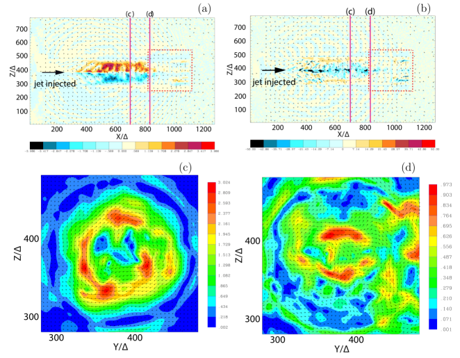
Figure 1: Upper panels: (a) the $y$-component of the magnetic field, $B_{\rm y}$, with $x$-$z$ electric field depicted by arrows, and (b) the $x$-component of the electron current density, $J_{\rm x}$, with the $x$-$z$ magnetic field as arrows, both in the $x-z$ plane at $t=1000\,\omega_{\rm pe}^{-1}$. The lower panels show the total magnetic-field strength in the $y-z$ plane at $x/\Delta=700$ (c) and $x/\Delta=835$ (d). The arrows indicate the magnetic field ($B_{\rm y},B_{\rm z}$).

The jet head blackassumed here has a flat-density top-hat shape which is a strong simplification of the true structure of the jet-formation region (e.g., Broderick & Loeb, 2009; Moscibrodzka et al., 2017). A more realistic jet structure (with, e.g., a Gaussian-shaped head) will be implemented in future studies.

The numerical code we use is a modified version of the relativistic electromagnetic PIC code TRISTAN (Buneman, 1993) with MPI-based parallelization (Niemiec et al., 2008). The simulations are performed in Cartesian coordinates on a numerical grid of size $(L_{x},L_{y},L_{z})=(1285\Delta,789\Delta,789\Delta)$. We use open boundaries at the $x/\Delta=0$ and $x/\Delta=1285$ surfaces and impose periodic boundary conditions in the transverse directions. Since the jet blackis located at the center of blackthe numerical box far from the boundaries and the simulation is rather short, blackthere are no visible effect of the periodic boundary conditions blackon the system.

The jet radius is $r_{\rm jet}=100\Delta$. The jet is injected at $x=100\Delta$ in the center of the $y-z$ plane. The large computational box allows us to follow the jet evolution blacklong enough to permit the investigation of the strongly nonlinear stage. The longitudinal box size, $L_{x}$, and the simulation time, $t_{\rm max}=1000\omega_{\rm pe}^{-1}$, are a factor of two larger than in our previous studies (Nishikawa et al., 2016b, 2017, 2019), in which jets with radii $r_{\rm jet}=20,40,80,120\Delta$ were investigated.

We know that jets of different plasma composition exhibit distinct dynamical behavior blackthat manifests itself in the morphologies of the jet and its emission characteristics (Nishikawa et al., 2016a, b, 2017, 2019). In this report blackwe discuss only electron-proton plasma in both the jet and the ambient medium. The initial blackparticle number per cell is $n_{\rm jt}=8$ and $n_{\rm am}=12$, respectively, for the jet and ambient plasma. The electron skin depth is $\lambda_{\rm se}=c/\omega_{\rm pe}=10.0\Delta$, where $c$ is the speed of light, $\omega_{\rm pe}=(e^{2}n_{\rm am}/\epsilon_{0}m_{\rm e})^{1/2}$ is the electron plasma frequency; the electron Debye length of ambient electrons is $\lambda_{\rm D}=0.5\Delta$. The blackthermal speed of jet electrons is $v_{\rm jt,th,e}=0.014c$ in the jet reference frame; in the ambient plasma it is $v_{\rm am,th,e}=0.03c$. blackWe assume temperature equilibration, and so the thermal speed of ions is smaller than that of electrons by the factor $(m_{\rm p}/m_{\rm e})^{1/2}$. We use the realistic proton-to-electron mass ratio $m_{\rm p}/m_{\rm e}=1836$. The jet plasma is initially weakly magnetized, and the magnetic field amplitude parameter assumed, $B_{0}=0.1c$, corresponds to plasma magnetization $\sigma=B^{2}/n_{\rm e}m_{\rm e}\gamma_{\rm jt}c^{2}=2.8\times 10^{-3}$. The jet Lorentz factor blackis $\gamma_{\rm jt}=15$.

3 Structure of Helically Magnetized Jets

Figure 1 shows cross-sections through the center of the jet at time $t=1000\,\omega_{\rm pe}^{-1}$ with (a) the $y$-component of the magnetic field, $B_{\rm y}$, with the $x$-$z$ electric field as arrows, and (b), the $x$-component of the electron current density, $J_{\rm x}$, with the $x$-$z$ magnetic field depicted as arrows. The jet propagates from the left to right. blackVery strong helical magnetic field in the jet is evident at $400\lesssim x/\Delta\lesssim 830$. The amplitude is with $B/B_{0}\approx 40$ (Fig. 1a) much larger than that of the initial field. As in the unmagnetized case (Nishikawa et al., 2016a), this field results from MI and kKHI. However, in the presence of the initial helical magnetic field the growth rate of the transverse MI mode is reduced, and the field structure is strongly modulated by longitudinal kKHI wave modes as shown by the bunched $B_{\rm y}$ field (Fig. 1a). This causes multiple collimations along the jet blackthat are caused by pinching of the jet electrons toward the center of the jet, as visible in the electron current density (Fig. 1b). It should be noted that blackin Fig 1b the color scale for $J_{\rm x}$ does not extend beyond $J_{\rm x}=-50$, as we intend to show the weak positive (return) current. blackThe collimations become weaker further along the jet and eventually disappear at $x/\Delta\gtrsim 830$. At this point $B_{\rm y}$ is weak. This demonstrates that the nonlinear saturation of the MI blackleads to the dissipation of the helical magnetic field.

blackWe selected possible reconnection sites in Figures 1a-b, indicated by the two red lines at $x/\Delta=700$ and $x/\Delta=835$, and show the magnetic-field structure in the $y-z$ plane in figure panels 1c and 1d, respectively.At $x/\Delta=700$ clockwise-circular magnetic field is split near the jet into a number of magnetic structures, which blackdemonstrate the growth of MI. They are surrounded by blackfield of opposite polarity that is produced by the proton current framing the jet boundary (see Nishikawa et al., 2016a). blackThe magnetic field at $x=835\Delta$ is strongly turbulent; its helical structure is distorted and reorganised into multiple magnetic islands, which reflect the nonlinear stage of MI and kKHI. The magnetic islands interact with each other, providing conditions for magnetic reconnection. In our 3D geometry reconnection does not occur at a simple X-point as in 2D slab geometry. Instead, reconnection sites can be identified with regions of weak magnetic field surrounded by oppositely directed magnetic field lines. An example of a possible location of reconnection can be found at $(y/\Delta,z/\Delta)=(380,340)$, where the total magnetic field becomes minimal (the null point, Fig. 1d). The evolution of the magnetic field at different locations in the jet ($600<x/\Delta<1100$) is shown in the supplemental movie. Note that the filamentary structure at the jet head (Fig. 1a-b) is formed by the electron WI. One can see in the movie that nonlinear evolution of the filaments also leads to the appearance of the magnetic structures that are prone to reconnection.

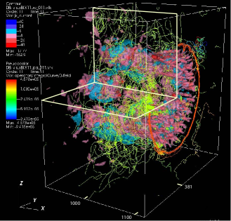
Figure 2: Isosurface of the $x$-component of the electron current density, $J_{\rm x}$, with the magnetic field lines black(yellow) in a rectangular section of the simulation grid ($920<x/\Delta<1120;231<y/\Delta,z/\Delta<531$) at time $t=1000\,\omega_{\rm pe}^{-1}$. To illustrate the blackdistribution of $J_{\rm x}$ inside the jet, a quadrant of the regions is clipped at the center of blackthe jet in the $x-z$ plane ($381<z/\Delta<531$) and in the $x-y$ plane ($231<y/\Delta<381$). The jet front is located at $x/\Delta=1100$.

(a)

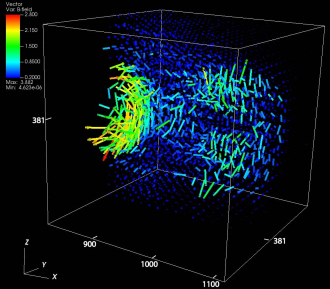
(b)

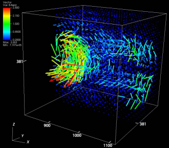
Figure 3: Magnetic-field vectors within a cubic section of the simulation grid ($820<x/\Delta<1120;231<y/\Delta,z/\Delta<531$) at time $t=900\,\omega_{\rm pe}^{-1}$ (a) and at $t=1000\,\omega_{\rm pe}^{-1}$ (b). To illustrate the magnetic field inside the jet, the plots show blackthe rear half of the jet with cut in the $x-z$ plane ($381<y/\Delta<531$).

blackIn Figure 2 we show three-dimensional isosurfaces of the $x$-component of the electron current density at the jet head together with magnetic field lines plotted in yellow. Two rectangles indicate the visible area in the jet. Near the jet head, the current filaments generated by the WI are blackevident. blackThis result is similar to that obtained by Ardaneh et al. (2016) (their Fig. 3), blackwho investigate the structure of the head of an electron-ion jet in slab geometry with $m_{\rm i}/m_{\rm e}=16$. They blackdemonstrated the acceleration of jet electrons in the linear stage of the instability. Figure 2 shows the merging of current components (the front of the nonlinear region) behind the current filaments, where some jet electrons are slightly accelerated, as we shall show in Fig. 4 below. More complicated structures are seen near the jet boundary, blackthat we shall investigate in more detail below.

The three-dimensional morphology of the jet’s magnetic field is shown in Figure 3 where we plot magnetic-field vectors at $t=900\,\omega_{\rm pe}^{-1}$ (Fig. 3a) and $t=1000\,\omega_{\rm pe}^{-1}$ (Figs. 3a and 3b). The regions displayed ($820<x/\Delta<1120;231<y/\Delta,z/\Delta<531$) are indicated by the red dashed rectangle in Figure 1b. The plot is clipped at the center of the jet at $y/\Delta=381$. One can see that the edge of the helical magnetic field in the jet moves from $x/\Delta=780$ at $t=900\,\omega_{\rm pe}^{-1}$ to $x/\Delta=830$ at $t=1000\,\omega_{\rm pe}^{-1}$, which is much slower than the jet speed black(if moving with the jet velocity, the front at $t=1000\,\omega_{\rm pe}^{-1}$ should be located at $x/\Delta\simeq 880$). This seems to indicate that the front edge of the helical magnetic field is peeled off as the jet propagates. This may indicate that the helical magnetic field is braided by kinetic instabilities and subsequently becomes untangled as discussed in Blandford et al. (2017). blackThe untangling of helical magnetic field results from magnetic-reconnection-like phenomena, that push the helical magnetic field blackaway from the center of the jet at the forward position. Two smaller magnetic islands can be identified in the jet shown in Figure 3 (half of the jet is shown). The blacksupplemental movie shows how the helical magnetic field is untangled and magnetic islands evolve along the jet at $t=1000\,\omega_{\rm pe}^{-1}$. For example at $x/\Delta=950$ the centers of magnetic islands are located around $(y/\Delta,z/\Delta)=$ (435, 420) (upper), (440, 318) (lower) (visible in Fig. 3b), (320,350), and (280, 400) (not visible).

Figure 4 shows the phase-space distribution of jet (red) and ambient (blue) electrons at $t=900\,\omega_{\rm pe}^{-1}$ and at $t=1000\,\omega_{\rm pe}^{-1}$. blackBoth groups of electrons are accelerated at several locations that coincide with jet recollimation regions (compare Fig. 1a-b). In particular, electrons are accelerated at $x/\Delta=780$, where the helical magnetic field disappears, as shown in Figure 3a. The disappearance of helical magnetic field near $x=830\Delta$ als coincides with the acceleration of electrons. blackAmbient electrons entrained in the relativistic jet plasma are also strongly accelerated.

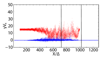
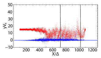
Figure 4: Phase-space ($x-\gamma V_{\rm x}$) distribution of jet (red) and ambient (blue) electrons at $t=900\,\omega_{\rm pe}^{-1}$ (top) and $t=1000\,\omega_{\rm pe}^{-1}$ (bottom). The two vertical lines show the regions blackfor which Fig. 3 displays the 3D magnetic-field vectors.

blackTo examine how electrons are accelerated in the jet, we plot in Fig. 5 their velocity distribution in the linear and the nonlinear stage. The jet electrons initially have a Lorentz factor $\gamma\simeq 15$. The distribution (in red) quickly widens, and some jet electrons are accelerated up to $\gamma=40$. Surprisingly, the ambient electrons can also be accelerated up to $\gamma=30$.

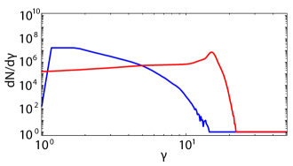
Figure 5: blackEnergy distributions of electrons in the region $x/\Delta<600$ (top panel) and $x/\Delta>600$ (bottom panel), corresponding to Fig. 4 at $t=1000\,\omega_{\rm pe}^{-1}$. The red and blue lines show the jet electron and ambient electron velocity distributions, respectively.

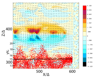
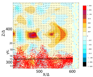
Figure 6: blackTop panel: Contours of $B_{\rm y}$ with arrows of $E_{\rm x,z}$. Bottom: $E_{\rm x}$ with arrows indicating $B_{\rm x,z}$. The $x-\gamma V_{\rm x}$ distribution of jet electrons at $t=500\,\omega_{\rm pe}^{-1}$ (a) is overplotted in red. Some jet electrons are accelerated up to $v_{\rm x}\gamma=20$ above the initial $v_{\rm x}\gamma=15$ (the black line) in the phase space. The scale for the phase-space is indicated with small digits at the left axis.

blackFigure 4 suggests that the groups of accelerated jet electrons visible at $t=900\,\omega_{\rm pe}^{-1}$ moved upward to larger $x$ at $t=1000\,\omega_{\rm pe}^{-1}$. These electrons were accelerated at an earlier time. blackTo investigate the process of their acceleration, in Figure 6 we show the correlation between electron acceleration and structures of the electromagnetic field excited by instabilities at $t=500\,\omega_{\rm pe}^{-1}$.

The MI is the dominant instability in the azimuthal direction. blackFigure 6 shows that it pinches blackthe jet and generates recollimation shocks. Certainly, kKHI is also excited, blackperturbs the jet, and aids in the creation of three recollimation shocks. blackFigure 6 features three regions with strong magnetic-field component $B_{\rm y}$, at which we can observe also a positive electric-field component $E_{\rm x}$. These structures are similar to recollimation shocks in RMHD simulations (Mizuno et al. 2014). blackThe arrows ($B_{\rm x},B_{\rm z}$)in Figure 6 indicate magnetic-field reversal at $(x/\Delta,z/\Delta)=(440,390)$. Reconnection in a 3D system is not easily identified in a 2D display, but the evidence in this figure and other diagnostics let’s us believe blackthat reconnection takes place. The sequence of evolution is blackthe following: kKHI and MI (WI) grow, and recollimation shocks are generated. At the same time reconnection occurs. blackThe negative quasi-static electric field $E_{\rm x}$ generated by the recollimation shocks accelerates jet electrons. blackElectrons are also decelerated where a strong positive $E_{\rm x}$ exists. blackWe note that the recollimation blackshocks are not as strong as blackshocks generated by the WI in slab geometry (compare, e.g., Ardaneh et al., 2016).

Note that electrons can be further accelerated to higher Lorentz factors on account of turbulent acceleration, as in kinetic simulations of driven magnetized turbulence (e.g., Comisso & Sironi, 2018; Zhdankin et al., 2018). In these simulations turbulent magnetic fluctuations are externally forced in the simulation system, and so the energy source for turbulence is not self-consistent. In contrast to the driven turbulence, in our simulations turbulent magnetic field (multiple magnetic-field islands) are self-consistently generated in the relativistic jet through the untangling of the helical magnetic field. Particles can be directly accelerated in the reconnection regions and also through interactions with the magnetic islands blackthat are visible in, e.g., Figure 1. The particle acceleration processes in turbulent magnetic reconnection have also been investigated by, e.g., Kowal et al. (2011, 2012); Lazarian et al. (2016).

4 Summary

We performed large-scale three-dimensional PIC simulations of an electron-proton jet containing helical magnetic fields. blackThe aim is to investigate in a systematic way how the helical magnetic field in jets evolves and accelerates electrons. The electron-proton jet undergoes kinetic instabilities, the most dominant of which is the MI. It pinches the jet and generates recollimation shocks. The kKHI also operates and contributes to the creation of recollimation shocks. We observed a number of instances of strong transverse magnetic field, $B_{\rm y}$, coinciding with significant jet-parallel electric field, $E_{\rm x}$, that are similar to the structure of recollimation shocks in RMHD simulations (Mizuno et al. 2014). Using as tracer magnetic-field reversals and other diagnostics, we found regions in which magnetic reconnection takes place.

blackIt appears that first kKHI and MI (WI) grow, then recollimation shocks are generated, and reconnection operates. The recollimation shocks feature a quasi-static electric field, $E_{\rm x}$, that depending on its sign accelerates or decelerates jet electrons. In the nonlinear stage the toroidal magnetic fields are untangled. The disappearance of helical magnetic fields generates magnetic field islands blackthat interact with each other and accelerate electrons. Kowal et al. (2011, 2012); Lazarian et al. (2016) blackinvestigated the particle acceleration process in turbulent reconnection theoretically and by numerical experiments. They blackdemonstrated an exponential growth in the energy of the accelerated particles and also the development of a power-law tail in the particle spectrum, blackboth of which are signatures of stochastic Fermi acceleration by reconnection. Figure 5 shows a power-law tail blackand hence is consistent with this scenario, but further investigation are needed to confirm stochastic Fermi acceleration.

Recently, de Gouveia Dal Pino et al. (2018); Kadowaki et al. (2018, 2019); Singh et al. (2016) blackused relativistic MHD simulations with test particles to investigate acceleration through turbulent magnetic reconnection driven by blackKI. blackUsing PIC simulations Alves et al. (2018, 2019) found that the formation of highly tangled magnetic fields and a large-scale inductive electric field in kink-unstable jets accelerates particles through curvature drift. There is no bulk flow in their simulations, blackand therefore velocity-shear instabilities such as kKHI and MI blackare not excited, blackand KI occurs instead. blackSince the magnetization in their simulations is very large, $\sigma>1$, the toroidal magnetic field is dominant and the KI is triggered, which tangles the helical magnetic field and consequently may result in reconnection, blackand not necessarily only curvature drift acceleration. blackWe should add that the jet density profile assumed in Alves et al. (2018), $n=n_{0}+(n_{\rm c}-n_{0})/\cosh^{2}(2r/R_{\rm c})$, differs from the top hat profile that we employ. Our choice may be more conducive to the kKHI, MI, and the Weibel modes.

Since kinetic KHI and MI grow faster than current-driven kink instabilities due to strong velocity shear and moderate magnetization, our simulation does not show a kink-like instability as seen in the simulations of Alves et al. (2018). In our simulation the particles are accelerated by the turbulent magnetic reconnection which is initiated by the growth of kinetic instabilities such as kKHI and MI.

blackWe investigated in a self-consistent fashion one of the possible mechanisms of electron acceleration in relativistic jets containing helical magnetic field. We demonstrated that as the electron-proton jet evolves, the helical magnetic field becomes untangled and locally reconnects. Electrons are accelerated within the resulting turbulent magnetic field. More simulations with larger jet radii are required, in which we vary the magnetic-field structures, for example the characteristic scale, $a$, and the pitch profile parameter, $\alpha$. Moreover, a variation of the density profile and the magnetization of the jet are required and will be the subject of future studies.

References

- Alves et al. (2015) Alves, E.P., Grismayer, T., Fonseca, R.A., Silva, L.O. 2015, Phys. Rev. E, 92, 021101
- Alves et al. (2018) Alves, E.P., Zrake, J., Fiuza, F., 2018, PRL 121, 245101
- Alves et al. (2019) Alves, E.P., Zrake, J., Fiuza, F., 2019, Phys. Plasmas 26, 072105
- Ardaneh et al. (2016) Ardaneh, K., Cai, D., Nishikawa, K.I. 2016, ApJ, 827, 124
- Barniol Duran et al. (2017) Barniol Duran, R., Tchekhovskoy, A., & Giannios, D. 2017, MNRAS 469, 4957
- Birkinshaw (1984) Birkinshaw, M. 1984, MNRAS, 208, 887
- Birkinshaw (1996) Birkinshaw, M. 1996, Astrophys Space Sci, 242: 17
- Blandford et al. (2017) Blandford, R., Yuan, Y., Hoshino, M., Sironi, L. 2017, Space Sci Rev, 207, 291
- Broderick & Loeb (2009) Broderick A. E. & Loeb A. 2009, ApJ, 697, 1164
- Buneman (1993) Buneman, O. 1993, in Computer Space Plasma Physics: Simulation Techniques and Software, Eds.: Matsumoto & Omura, Tokyo: Terra, p.67
- Christie et al. (2019) Christie, I. M., Lalakos, A., Tchekhovskoy, A., Fern ndez, R., Foucart, F., Quataert, E., Kasen, D. 2019, MNRAS, 490, 4811
- Comisso & Sironi (2018) Comisso, L., Sironi, L., 2018, prl, 121, 255101
- Daughton (2011) Daughton, W., Roytershteyn, V., Karimabadi, H., et al. 2011, Physics Nature, 7, 539
- de Gouveia Dal Pino & Lazarian (2005) de Gouveia Dal Pino, E. M., & Lazarian, A. 2005, A&A 441, 845
- de Gouveia Dal Pino et al. (2010) de Gouveia Dal Pino, E. M., Piovezan, P. P., Kadowaki, L. H. S. 2010, A&A, 518, 5
- de Gouveia Dal Pino et al. (2018) de Gouveia Dal Pino, E. M., Alves Batista, R., Kowal, G., Medina-Torrej n, T., Ramirez-Rodriguez, J. C. 2018, https://pos.sissa.it/cgi-bin/reader/conf.cgi?confid=329
- Drenkhahn & Spruit (2002) Drenkhahn, G., & Spruit, H. C. 2002, A&A 391, 1141
- Fowler et al. (2019) Fowler, T. K., Li, H., Anantua, R. 2019, ApJ, 885, 4
- Fujjimoto (2011) Fujjimoto, K. 2011, J. Compt. Phys., 230, 8508
- Gabuzda (2019) Gabuzda,D., 2019, Galaxies, 7, 5
- Giannios et al. (2009) Giannios, D., Uzdensky, D. A., & Begelman, M. C., MNRAS, 395, L29
- Giannios (2010) Giannios, D. 2010, MNRAS, 408, L46
- Giannios (2011) Giannios, D. 2011, J. Phys: Conf. Ser. 283, 012015
- Granot et al. (2011) Granot, J., Komissarov, S. S., & Spitkovsky, A. 2011, MNRAS, 411, 1323
- Granot (2012) Granot, J. 2012, MNRAS, 421, 2442
- Guo et al. (2015) Guo, F., Liu, Y.-H., Daughton, W., & Li, H., 2015, ApJ, 806, 167
- Guo et al. (2016a) Guo, F., Li, H., Daughton, W., et al., 2016a, ApJL, 818, L9
- Guo et al. (2016b) Guo, F., Li, H., Daughton, W., Li, X., & Liu, Y.-H., 2016b, PhPl, 23, 5708
- Hawley et al. (2015) Hawley, J. F., Fendt, C., Hardcastle, M., et al. 2015, Space Sci. Rev., 191, 441
- Kadowaki et al. (2018) Kadowaki, L. H. S.; De Gouveia Dal Pino, E. M., Stone, J. M. 2018, ApJ, 864, 52
- Kadowaki et al. (2019) Kadowaki, L. H. S., de Gouveia Dal Pino, E. M., Medina-Torrej n, T. E. 2019, https://pos.sissa.it/cgi-bin/reader/conf.cgi?confid=329
- Kagan et al. (2013) Kagan, D., Milosavljevic, M., & Spitkovsky, A. 2013, ApJ, 774, 41
- Karimabadi et al. (2014) Karimabadi, H., Roytershteyn, V., Vu, H. X., et al. 2014, PhPl, 21, 2308
- Komissarov (2012) Komissarov, S. S. 2012, MNRAS, 422, 326
- Kowal et al. (2011) Kowal, G., de Gouveia Dal Pino, E.M., Lazarian, A. 2011, ApJ. 735, 102
- Kowal et al. (2012) Kowal, G., de Gouveia Dal Pino, E. M., Lazarian, A., 2012, Phys. Rev. Lett., 108, 241102
- Lazarian et al. (2016) Lazarian A., Kowal G., Takamoto M., de Gouveia Dal Pino E.M., Cho J. 2016, Theory and Applications of Non-relativistic and Relativistic Turbulent Reconnection. In: Gonzalez W., Parker E. (eds) Magnetic Reconnection. Astrophysics and Space Science Library, vol 427. Springer, Cham
- Markidis et al. (2014) Markidis, S., Lapenta, G. Delzanno, G. L., et al. 2014, PPCF, 56, 064010
- McKinney & Uzdensky (2012) McKinney, J. C., & Uzdensky, D. A. 2012, MNRAS, 419, 573
- Mizuno et al. (2014) Mizuno, Y., Hardee, P. E., & Nishikawa, K.-I. 2014, ApJ, 784, 167
- Moscibrodzka et al. (2017) Mościbrodzka, M., Dexter, J., Davelaar, J., & Falcke, H., MNRAS, 468, 221
- Niemiec et al. (2008) Niemiec, J., Pohl, M., Stroman, T., & Nishikawa, K.-I. 2008, ApJ, 684, 1174-1189
- Nishikawa et al. (2016a) Nishikawa, K.-I., Frederiksen, J. T., Nordlund, Å., et al. 2016a, ApJ, 820, 94
- Nishikawa et al. (2016b) Nishikawa, K.-I., Mizuno, Y., Niemiec, J., et al. 2016b, Galaxies, 4, 38
- Nishikawa et al. (2017) Nishikawa, K.-I., Mizuno, Y., Gómez, J. L., et al. 2017, Galaxies, 5, 58
- Nishikawa et al. (2019) Nishikawa, K.-I., Mizuno, Y., Gómez, J. L., et al. 2019, Galaxies, 7, 29
- Oka et al. (2008) Oka, M., Fujimoto, T. K., Nakamura, M., et al. 2008, PRL, 101, 205004
- Singh et al. (2016) Singh, C. B., Mizuno, Y., & de Gouveia Dal Pino, E., 2016, ApJ, 824, 48
- Sironi & Spitkovsky (2011) Sironi, L. & Spitkovsky, A. 2011, ApJ, 741, 39
- Sironi et al. (2013) Sironi, L., Spitkovsky, A., Arons, J. 2013, ApJ, 771, 54.
- Sironi & Spitkovsky (2014) Sironi, L. & Spitkovsky, A. 2014, ApJ, 783, L21
- Sironi et al. (2015) Sironi, L., Petropoulou, M., & Giannios, D. 2015, MNRAS, 450, 183
- Stone & Norman (1994) Stone, J. M. & Morman, M. L. 1994, ApJ, 433, 746. Stone, James M.; Norman, Michael L.
- Stone & Hardee (2000) Stone, J. M., Hardee, Philip E. 2000, ApJ, 540, 192
- Tchekhovskoy (2015) Tchekhovskoy, A. 2015, ASSL, 414, 45
- Uzdensky (2011) Uzdensky, D. A. 2011, Space Sci. Rev., 160, 45
- Wendel et al. (2013) Wendel, D. E., Olson, D. K., Hesse, M., et al. 2013, PhPl, 20, 2105
- Yao et al. (2019) Yao, W., Qiao, B., Zhao, Z., Lei, Z., Zhang, H., Zhou, C., Zhu, S., He1, X., 2019, ApJ, 876, 2
- Zenitani & Hoshino (2005) Zenitani, S. & Hoshino, M. 2005, ApJ, 618, L111
- Zenitani & Hoshino (2008) Zenitani, S. & Hoshino, M. 2008, ApJ, 677, 530
- Zenitani et al. (2011) Zenitani, S., Hesse, M., Klimas, A., & Kuznetsova, M. 2011, PRL, 106, 195003
- Zenitani et al. (2013) Zenitani, S., Shinohara, I., Nagai, T., & Wada, T. 2013, PhPl, 20, 092120
- Zhang & Yan (2011) Zhang, B. & Yan, H. 2011, ApJ, 726, 90
- Zhdankin et al. (2018) Zhdankin, V., Uzdensky, D. A., Werner, G. R., Begelman, M. C., 2018, ApJL, 867, L18