Conical Holographic Heat Engines

Abstract

We demonstrate that adding a conical deficit to a black hole holographic heat engine increases its efficiency; in contrast, allowing a black hole to accelerate decreases efficiency if the same average conical deficit is maintained. Adding other charges to the black hole does not change this qualitative effect. We also present a simple formula to calculate the efficiency of elliptical cycles for any $C_{V}\neq 0$ black hole, which allows a more efficient numerical algorithm for computation.

1 Introduction

As a consequence of the holographic principle, asymptotically anti-de Sitter (AdS) black hole solutions have grown into fruitful playgrounds in which to explore aspects of both quantum gravity and strongly coupled gauge field theories (see e.g. Maldacena:1997re ; Gubser:1998bc ; Witten:1998qj ; Chamblin:1999tk ; Freedman:1999gp ; Caldarelli:1999xj ; Myers:2010xs ). Attempts to formulate a consistent thermodynamic description of such objects, building on the seminal work of Hawking and Page Hawking:1982dh , have not only led to relations suggestive of dualities between gravitational thermodynamic processes and renormalisation group flows in finite temperature quantum field theories Casini:2011kv ; Johnson:2018amj , they have spawned an entirely new field of investigation, known as black hole chemistry. (For a review this subject, the authors recommend Kubiznak:2016qmn ).

In the extended thermodynamics formalism, a dynamical negative cosmological “constant” $\Lambda$ is promoted to a thermodynamic variable of the black hole Henneaux:1984ji ; Teitelboim:1985dp , interpreted as a positive pressure $P=-\Lambda/8\pi$. Alongside it’s conjugate potential, the thermodynamic volume $V$, and the usual identifications of horizon area with entropy $S$ and surface gravity with temperature $T$, the first law of black hole mechanics takes a form reminiscent of the first law of thermodynamics for a more traditional system:

$$dM=TdS+VdP+\ldots.$$ (1)

The presence of the $VdP$ term (as opposed to $-PdV$) indicates that the black hole ‘mass’ $M$, while historically being associated with internal energy, has a more correct interpretation of enthalpy Kastor:2009wy , see also Dolan:2010ha ; Dolan:2011xt ; Kubiznak:2012wp ; Dolan:2012jh .

Such a setup has led to the identification of a wide variety of thermodynamic phenomena, including entropy inequalities Cvetic:2010jb ; Dolan:2013ft , Van der Waals-like behaviour Kubiznak:2012wp ; Gregory:2019dtq , triple points Altamirano:2013uqa , reentrant phase transitions Gunasekaran:2012dq , and analogous behaviour to superfluidity transitions present in condensed matter systems Hennigar:2016xwd . Further, suggestions have been made that pressure variations in the bulk might correspond to a variation in a “chemical potential” associated to the number of colours in the dual CFT Kastor:2014dra ; Dolan:2014cja or to its volume when the number of colours is held fixed Karch:2015rpa .

A natural question to pose in light of these developments is whether it is possible to construct thermodynamic cycles using these extended thermodynamics that one can traverse to extract mechanical work. In a series of papers, Johnson and collaborators have fleshed out this proposal Johnson:2014yja ; Johnson:2016pfa ; Chakraborty:2016ssb ; Chakraborty:2017weq ; Rosso:2018acz ; Johnson:2019olt , exploring not only the concept of a holographic heat engine, but deriving their properties, exact expressions and bounds on efficiencies Johnson:2014yja ; Johnson:2016pfa ; Rosso:2018acz . Since the choice of black hole solution provides the working substance for such an engine, it is sensible to compare how the choice of solution impacts the efficiency of a given cycle.

Naïvely, one might consider a simple rectangular cycle in the $V$–$P$ plane (consisting of two isobars and two isochores) or a Carnot cycle (consisting of two isobars and two adiabats) as appropriate for this comparison. Indeed, the efficiency of a rectangular cycle for static black holes is readily obtained in exact analytic form by Johnson Johnson:2016pfa , that was then extended to a general rotating black hole in the canonical ensemble by Hennigar et al. Hennigar:2017apu , who presented the efficiency in a simple geometric form. However, it was suggested by Chakraborty and Johnson that these cycles may favour certain black hole solutions Chakraborty:2016ssb ; Chakraborty:2017weq due to the particular form of the associated equation of state. In order to determine which working substances produce the most efficient engines, they proposed that a fair comparison can be performed by calculating the efficiencies of elliptical cycles instead, as these are in some sense “equally unfavourable” for all black hole solutions.

In this paper, we re-examine this benchmarking scheme as applied to black holes with conical deficits. Efforts to acquire exact expressions for the efficiency of the required elliptical cycles have hitherto been limited to the class of solutions with vanishing specific heat at constant volume $C_{V}=0$ Rosso:2018acz , for which there can be no rotational charge Hennigar:2017apu and the sets of isochores and adiabats are identical. We show that it is possible to write down an exact expression for the efficiency of an elliptical cycle in the $V$–$P$ plane, in the canonical ensemble, for a general $C_{V}\neq 0$ black hole. The result takes a pleasant geometric form and provides an efficient algorithm with which to calculate efficiency.

Using this result and numerical investigation, we give a discussion of the effect of various thermodynamic charges for a class of asymptotically-AdS solutions to four dimensional Einstein gravity describing an accelerating, rotating, electrically charged black hole. We also consider the impact of shifting the position of the benchmarking cycle in the $P$–$V$ plane. Accelerating black holes in the benchmarking framework have been briefly investigated by Zhang et al. Zhang:2018vqs ; Zhang:2018hms , although in their study the thermodynamics have been unjustly constrained by a choice to remove the tension from one of the polar axes. We find that it is the average of the “north” and “south” polar tensions that comes to dominate cycle efficiency over the acceleration induced by their differential. The overzealous constraining of the thermodynamic charges has meant that this fact has, thus far, gone unnoticed.

The paper is organised as follows: in section 2 we review the thermodynamics of the metric representing a charged, rotating, slowly-accelerating, (asymptotically AdS) black hole. In doing so, we derive a novel bound on the metric parameters. In section 3 we present an exact expression for the efficiency of an elliptical benchmarking cycle showing how this provides an efficient algorithm to calculate efficiency to a high degree of precision. In section 4 we discuss the benchmarking scheme as applied to these accelerating black holes, evaluating the impact of conical deficits and extent to which changes in efficiency may be attributed to acceleration. Finally, in section 5 we discuss general features of the impact of position and geometry of benchmarking cycles on efficiency and conclude.

2 Thermodynamics of the Charged, Rotating C-Metric

We begin by reviewing the thermodynamics of the charged, rotating C-metric Anabalon:2018ydc ; Anabalon:2018qfv , see also Appels:2016uha ; Appels:2017xoe ; Gregory:2017ogk ; Astorino:2016xiy ; Astorino:2016ybm ; MikeThesis ; Dutta:2005iy , which is given in Boyer-Lindquist type coordinates Kinnersley:1970zw ; Plebanski:1976gy ; Griffiths:2005qp as

$$ds^{2}=\frac{1}{H^{2}}\Bigg{[}- \frac{f(r)}{\Sigma}\left(\frac{dt}{\alpha}+a\sin^{2}(\theta)\frac{d\phi}{K}\right)^{2}+\frac{\Sigma}{f(r)}dr^{2}$$ (2)

$$+ \frac{r^{2}\Sigma}{g(\theta)}d\theta^{2}+\frac{g(\theta)\sin^{2}(\theta)}{r^{2}\Sigma}\left(\frac{a}{\alpha}dt-(r^{2}+a^{2})\frac{d\theta}{K}\right)^{2}\Bigg{]}\,.$$

Where the $U(1)$ field strength

$$F=dB\,,\qquad B=-\frac{e}{r\Sigma}\left[\frac{dt}{\alpha}-a\sin^{2}\theta\frac{d\phi}{K}\right]+\frac{er_{+}dt}{(a^{2}+r_{+}^{2})\alpha}\,,$$ (3)

is suitably chosen such that the gauge potential vanishes at the black hole horizon. An explicit factor of $K$ has been included so that the azimuthal coordinate $\phi$ has periodicity $2\pi$. $K$ typically tracks the presence of conical deficits in the spacetime, as explained below, thus has physical content, however $\alpha$, the rescaling of the time coordinate, is not a free parameter in the metric, but is dependent on the other parameters (as defined in (12)) and is introduced to appropriately renormalise the timelike killing vector $\partial_{t}$ as described in Anabalon:2018ydc ; Anabalon:2018qfv . The remaining metric functions on this patch are given by

$$f(r) =(1-A^{2}r^{2})\left[1-\frac{2m}{r}+\frac{a^{2}+e^{2}}{r^{2}}\right]+\frac{r^{2}+a^{2}}{\ell^{2}}\,,$$ (4)

$$g(\theta) =1+2mA\cos\theta+(\Xi-1)\cos^{2}\theta\,,$$

$$\Sigma =1+\frac{a^{2}}{r^{2}}\cos^{2}\theta\,,\qquad H=1+Ar\cos\theta\,,$$

$$\Xi =1+e^{2}A^{2}-\frac{a^{2}}{\ell^{2}}(1-A^{2}\ell^{2})\,.$$

The presence (or not) of conical deficits is revealed by expanding the angular part of the metric near each axis. Such deficits are interpreted as cosmic strings emerging from the black hole Aryal:1986sz , as the conical deficits can be smoothed out by a typical cosmic string core Gregory:1995hd ; Achucarro:1995nu ; Gregory:2013xca ; Gregory:2014uca . The tension of the string, $\mu$, is related to the deficit $\delta$ via $\delta=8\pi\mu$. Calculating the deficits along the North ($+$) and South ($-$) axes gives:

$$\mu_{\pm}=\frac{\delta_{\pm}}{8\pi}=\frac{1}{4}\left[1-\frac{\Xi\pm 2mA}{K}\right]\,.$$ (5)

As is common, and without loss of generality, we take a non-negative acceleration parameter $A$ so that $\mu_{-}\geq\mu_{+}$. Often, $\mu_{+}$ is set to zero so that the North axis is regular, however we do not wish to entangle the physics of deficits with the physics of acceleration, so will not restrict ourselves thus, but instead will allow both tensions to vary. Following Gregory:2019dtq , we express the tensions in terms of the average and differential quantities $\Delta$ and $C$:

$$\Delta=1-2(\mu_{-}+\mu_{+})=\frac{\Xi}{K}\,,\qquad\quad C=\frac{\delta\mu}{\Delta}=\frac{\mu_{-}-\mu_{+}}{\Delta}=\frac{mA}{\Xi}\,,$$ (6)

in order to present the discussion of thermodynamics, although we use both $C$ and $\delta\mu$ when discussing the impact of acceleration. Note that these variables are no longer completely unconstrained; for example, $\delta\mu$ must vanish for $\Delta=1$. Specifically, requiring positive tensions and acceleration then gives a bound on the magnitude of acceleration:

$$C<\begin{cases}1/2\,,&\text{for $0<\Delta\leq 1/2$,}\\ \frac{1-\Delta}{2\Delta}\,,&\text{for $1/2<\Delta\leq 1$.}\end{cases}$$ (7)

It is worth reiterating the relation between the physics of acceleration and that of deficits. A black hole can have a conical deficit without accelerating, and $\Delta$ encodes this property, however, note that $\Delta=1$ for zero deficit and acceleration, then drops as the conical deficit average increases. $C$ increases as acceleration increases, saturating at $C=1/2$ for a critical black hole, defined as having a deficit of $2\pi$ along the South axis. Since it is not possible for the deficit to increase further, $C$ remains at $1/2$ independent of the North pole deficit, but the acceleration of the black hole drops as $\mu_{+}$ increases, returning to zero as $\mu_{+}\to\mu_{-}$ and $\Delta\to 0$. Therefore, while $C$ is a convenient parameter to express the extensive thermodynamical variables Gregory:2019dtq , $\delta\mu$ is more representative of acceleration and we will frequently use it for displaying results.

At this point, it is worth commenting on the parametric restrictions in the metric. Positivity of the conformal factor $H=1+Ar\cos\theta$, constrains $Ar\cos\theta<1$ and sets the location of the conformal boundary $r_{\text{bd.}}=-1/A\cos\theta$. Our main assumption is that the black hole is slowly accelerating, (see Podolsky:2002nk for a full discussion) i.e. its time coordinate is proportional to the asymptotic time for an observer near the boundary. For the black hole to also be isolated (i.e. the only event horizon being that of the black hole) we require no zeros of $g_{tt}$, or $f$, on the boundary. Finally, for $\theta=0,\pi$ to represent the poles, we require $g(\theta)>0$ on $[0,\pi]$. All these requirements lead to a set of intersecting constraints on the parameters.

First, $g\geq 0$ gives a bound on the possible values of the dimensionless mass:

$$mA<\begin{cases}\Xi/2,&\text{for $\Xi\in(0,2]$,}\\ \sqrt{\Xi-1},&\text{for $\Xi>2$.}\end{cases}$$ (8)

However, the fact that the black hole horizon does not intersect the boundary requires $Ar_{+}<1$, hence the Kerr-Newman potential multiplying $(1-A^{2}r_{+}^{2})$ in $f(r_{+})=0$ must be negative. This in turn requires

$$m^{2}>a^{2}+e^{2}\qquad\Rightarrow\qquad m^{2}A^{2}>\Xi-1+\frac{a^{2}}{\ell^{2}}>\Xi-1\,.$$ (9)

Thus, by comparison with (8), we see that $\Xi>2$ is not allowed. Hence

$$mA\leq\frac{\Xi}{2}<1.$$ (10)

The condition for slow acceleration, or $f>0$ on the boundary, then becomes an algebraic constraint on the parameters, that must be satisfied in conjunction with the existence of a black hole horizon. This is a rather involved set of constraints which are most easily solved numerically. We refer the reader to MikeThesis for a fuller discussion.

Consistent thermodynamic parameters for this class of solutions have been identified in Anabalon:2018qfv by promoting $\mu_{\pm}$ to thermodynamic charges, taken together with their conjugate thermodynamic lengths $\lambda_{\pm}$. We restate them here for clarity:

$$M =\frac{m(\Xi+a^{2}/\ell^{2})(1-A^{2}\ell^{2}\Xi)}{K\Xi\alpha(1+a^{2}A^{2})}\,,$$ (11)

$$T =\frac{f^{\prime}_{+}r_{+}^{2}}{4\pi\alpha(r_{+}^{2}+a^{2})}\,,\qquad S=\frac{\pi(r_{+}^{2}+a^{2})}{K(1-A^{2}r_{+}^{2})}\,,$$

$$Q =\frac{e}{K}\,,\quad\Phi=\Phi_{t}=\frac{er_{+}}{(r_{+}^{2}+a^{2})\alpha}\,,$$

$$J =\frac{ma}{K^{2}}\,,\quad\Omega=\Omega_{H}-\Omega_{\infty}\,=\left(\frac{Ka}{\alpha(r_{+}^{2}+a^{2})}\right)-\left(-\frac{aK(1-A^{2}\ell^{2}\Xi)}{\ell^{2}\Xi\alpha(1+a^{2}A^{2})}\right)\,,$$

$$P =\frac{3}{8\pi\ell^{2}}\,,\quad V=\frac{4\pi}{3K\alpha}\left[\frac{r_{+}(r_{+}^{2}+a^{2})}{(1-A^{2}r_{+}^{2})^{2}}+\frac{m[a^{2}(1-A^{2}\ell^{2}\Xi)+A^{2}\ell^{4}\Xi(\Xi+a^{2}/\ell^{2})]}{(1+a^{2}A^{2})\Xi}\right]\,,$$

$$\lambda_{\pm} =\frac{-r_{+}}{\alpha(1\pm Ar_{+})}+\frac{m}{\alpha}\frac{[\Xi+a^{2}/\ell^{2}+\frac{a^{2}}{\ell^{2}}(1-A^{2}\ell^{2}\Xi)]}{(1+a^{2}A^{2})\Xi^{2}}\pm\frac{A\ell^{2}(\Xi+a^{2}/\ell^{2})}{\alpha(1+a^{2}A^{2})}\,,$$

with the correct normalisation of the timelike killing vector given by

$$\alpha=\frac{\sqrt{(\Xi+a^{2}/l^{2})(1-A^{2}l^{2}\Xi)}}{1+a^{2}A^{2}}\,.$$ (12)

The parameters (11) were shown to satisfy both an extended first law of thermodynamics

$$dM=TdS+VdP+\Omega dJ+\Phi dQ+\lambda_{+}d\mu_{+}+\lambda_{-}d\mu_{-}\,,$$ (13)

and Smarr relation Smarr:1972kt

$$M=2(TS-PV+\Omega J)+\Phi Q\,.$$ (14)

Interesting thermodynamic behaviour – including zeroth, first, and second order phase transitions and the first example of a reentrant black hole phase transion when $P$ is varied – of these solutions has been discussed in the literature Abbasvandi:2018vsh ; Abbasvandi:2019vfz . It is also possible to rewrite the expressions (11) in terms of the thermodynamic charges Gregory:2019dtq :

$$V =\frac{2S^{2}}{3\pi M}\left[\left(1+\frac{\pi Q^{2}}{\Delta S}+\frac{8PS}{3\Delta}\right)+2\left(\frac{\pi J}{\Delta S}\right)^{2}+2\left(\frac{3\Delta C}{8PS}\right)^{2}\right]\,,$$ (15)

$$T =\frac{\Delta}{8\pi M}\Bigg{[}\left(1+\frac{\pi Q^{2}}{\Delta S}+\frac{8PS}{3\Delta}\right)\left(1-\frac{\pi Q^{2}}{\Delta S}+\frac{8PS}{\Delta}\right)-4\left(\frac{\pi J}{\Delta S}\right)^{2}-{4C^{2}}\Bigg{]}\,,$$

$$\Omega =\frac{\pi J}{SM\Delta}\left(1+\frac{8PS}{3\Delta}\right)\,,$$

$$\Phi =\frac{Q}{2M}\left(1+\frac{\pi Q^{2}}{S\Delta}+\frac{8PS}{3\Delta}\right)\,,$$

$$\lambda_{\pm} =\frac{-S}{\pi M}\Bigg{[}\!\!\left(\!\frac{4PS}{3\Delta}+\frac{\pi Q^{2}}{2\Delta S}\!\right)^{2}\!\!+\frac{\pi^{2}J^{2}}{\Delta^{2}S^{2}}\left(\!1+\frac{16PS}{3\Delta}\!\right)\!-\left(1\mp{2C}\right)^{2}\pm 4\left(\frac{3\Delta C}{8PS}\right)\!\Bigg{]}$$

giving a generalisation of the Christodoulou-Ruffini formula Christodoulou:1972kt ; Caldarelli:1999xj for enthalpy:

$$M^{2}=\frac{\Delta S}{4\pi}\left[\left(1+\frac{\pi Q^{2}}{\Delta S}+\frac{8PS}{3\Delta}\right)^{2}+4\left(1+\frac{8PS}{3\Delta}\right)\left\{\left(\frac{\pi J}{\Delta S}\right)^{2}-\frac{3\Delta C^{2}}{8PS}\right\}\right]\,.$$ (16)

Having expressions purely in terms of extensive quantities clarifies the chemical interpretation of black holes, and enables a more straightforward analysis of the properties of accelerating heat engines.

These expressions make it clear that the reverse isoperimetric inequality Cvetic:2010jb is satisfied for this class of solutions Gregory:2019dtq .

3 An Exact Efficiency Formula for Circular Cycles

As discussed in the introduction, previous authors have calculated the efficiency of elliptical benchmarking cycles for black hole solutions with $C_{V}=0$. However, it is possible to make a more general statement, extending this result to a broader class of solutions.

Recall that an engine consists of a cycle that has a “cool” component, where work is extracted, and a “hot” component, where the engine is refuelled. The efficiency is simply the ratio of overall heat extracted to the heat put in, where the heat flow is given by an integral

$$Q=\int TdS$$ (17)

over each component of the cycle. The transition between the hot and cold parts of the cycle occurs when $\delta S=0$. Thus, on any cycle in the $(V,P)$ plane, the turning points of $S$ must be determined. The trickiness of the problem now becomes apparent, as the thermodynamic variables are most readily given in terms of the charges $S,P,\ldots$, whereas we require $M(P,V)$ so that we can determine the stationary points of $S$.

Two common simple cycles used are the Carnot, and a $(V,P)$–rectangular cycle. These have clear turning points for $S$ at the corners. However, while the rectangular cycle is easy to use for black holes with conical deficits, it turns out that the Carnot cycle is not. The Carnot cycle consists of adiabats and isotherms. The engine is first heated up, by increasing the pressure at fixed volume, then allowed to expand at constant temperature. The cycle then completes by cooling to the original temperature by dropping the pressure, and contracting to the original $P$ and $V$ at constant $T$. The geometry of the Carnot cycle therefore depends crucially on the isotherms of the system. Looking at (16) we see a scaling symmetry,

$$\hat{S}=\Delta S\,,\qquad\hat{P}=P/\Delta^{2}\,,$$ (18)

so that

$$V=\frac{\hat{V}(\hat{S},\hat{P})}{\Delta^{2}}\,,\qquad T=\Delta\hat{T}(\hat{S},\hat{P})\,,$$ (19)

where $\hat{T}$, $\hat{V}$ are the expressions for the undeficited black hole. Thus, irrespective of any impact of acceleration, turning on a conical deficit gives a transformation on the $(V,P)$ plane, and not only distorts, but rescales, the isotherms. For a Carnot engine cycling between the same two temperatures and entropies, the addition of a deficit “drops the pressure” of the cycle, lowering the maximum pressure obtained. By looking at the expressions (15) for $T$ and $V$, one can deduce that both quantities are only significantly altered by the addition of the terms containing $C$ when both $T$ and $V$ are small. These effects are depicted in figure 1, showing Carnot engines for a “vanilla” (uncharged nonrotating) black hole cycling between the same two temperatures and entropies. First an average deficit $\Delta=0.5$ is added (solid red), and can be seen to have a strong effect on the geometry of the cycle, however, when the maximum possible thermodynamic acceleration, $\delta\mu=0.25$ or $C=0.5$, is added (still having the same average deficit $\Delta=0.5$) the cycle changes very little. As is the case generally, the presence of the deficit dominates the phase-space position and shape of the cycle, with the deformation due to acceleration only becoming non-negligible at small $V$ and $P$.

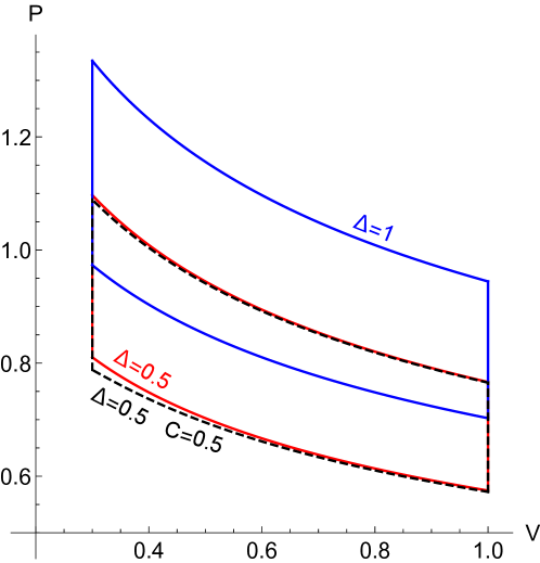
Figure 1: An illustration of the impact of conical deficits and acceleration on the Carnot cycle of an uncharged nonrotating black hole.The cycles have upper (lower) temperature $T=1.3$ ($1.0$) and maximum (minimum) volume $V=1.0$ ($0.3$). First an average deficit $\Delta=0.5$ is added (solid red), and can be seen to have a strong effect on the geometry of the cycle, however, when the maximum possible thermodynamic acceleration, $\delta\mu=0.25$, $C=0.5$, is added (still having the same average deficit $\Delta=0.5$) the cycle changes very little.

Since introducing a deficit distorts and rescales the isotherms needed to construct Carnot cycles, it is necessary to instead use a geometrically fixed benchmarking cycle. Rectangular cycles are relatively straightforward. Indeed, an exact formula for their efficiency for any black hole was given in Hennigar:2017apu :

$$\eta=\frac{\Delta V\Delta P}{\Delta M_{T}+\Delta U_{L}}\,,$$ (20)

where $\Delta M_{T}$ is the difference in enthalpy between the top-right and top-left corners of the cycle in the $(V,P)$-plane, and $\Delta U_{L}$ is the difference in internal energy $U=M-PV$ between the top-left and bottom-left corners. For the vanilla C-metric, this evaluates to

$$\eta=\frac{2A}{A+2P_{0}\Delta V+\left(\frac{3\Delta^{2}}{4\pi}\right)^{\frac{1}{3}}\left(V_{R}^{\frac{1}{3}}-V_{L}^{\frac{1}{3}}\right)}+\mathcal{O}(C^{2})\,,$$ (21)

where $A=\Delta V\Delta P$ is the area of the cycle; $V_{R}$ and $V_{L}$ are the maximum and minimum volumes attained respectively; and $P_{0}$ is the pressure at the cycle’s centroid. The correction of order $C^{2}$ is calculated by resorting to the expansion (32) which we present later in our analysis of circular cycles.

Adding a deficit (i.e. lowering $\Delta$) acts to increase the efficiency of rectangular cycles. When calculated, the correction from acceleration decreases the efficiency again, albeit by a lesser amount. These effects are demonstrated in figure 2 wherein the efficiency of a typical rectangular cycle is plotted against $\Delta$ for various values of $C$. Here we see how increasing the deficit (corresponding slightly counterintuitively by moving to the left in the plot) increases efficiency. Adding acceleration via $C$ on the other hand lowers efficiency, as can be seen from the coloured dashed/dotted lines lying below the black $\delta\mu=0$ curve.

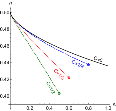
Figure 2: The efficiency of a typical rectangular cycle with maximum (minimum) pressure $P=1.0$ ($0.5$) and volume $V=1$ ($0.5$), for a $Q=J=0$ solution. The non-accelerating case is shown in solid black. Cases with three values of non-zero $C$ are plotted using broken curves, up to the maximum legal $\Delta$. Increasing the average deficit (dropping $\Delta$) is seen to increase efficiency. Greater values of acceleration are seen to give reduced efficiency.

As discussed in the introduction, previous authors Rosso:2018acz ; Chakraborty:2016ssb ; Chakraborty:2017weq have also calculated the efficiency of circular benchmarking cycles for black hole solutions with $C_{V}=0$. However, we can use the first law to give a more general geometric expression for the efficiency for any black hole heat engine, even those with non-vanishing specific heat. Consider for convenience a circular benchmarking cycle defined parametrically by

$$V(\theta) =V_{0}+R\cos{\theta}\,,$$ (22)

$$P(\theta) =P_{0}-R\sin{\theta}\,.$$

Here, $(V_{0},P_{0})$ indicates the centre of the cycle and $R$ its radius. Calculating the work done in traversing the circle is in principle straightforward as, in the canonical ensemble, the heat flow is given simply by the first law:

$$\delta Q =TdS=dM-VdP\,,$$ (23)

$$\implies Q =\Delta M-\int VdP\,.$$

In general the presence of charges means that isochores are no longer adiabats, and the turning points of $S$ along the circle are displaced from the symmetric position (see figure 3), however the first law integral (23) is still applicable and we may write the integrals for $Q_{C}$ and $Q_{H}$ as simple combinations of mass differentials and areas of regions in the circle. Assuming the turning points $\theta_{1,2}$ divide the circle into two segments, with areas $C_{1}$ and $C_{2}$, above and below the chords parallel to the $V$–axis defined by $\theta_{1}$ and $\theta_{2}$ respectively, the strip of the circle remaining has area ${\cal S}=\pi R^{2}-C_{1}-C_{2}$. These regions are shown in figure 3. Inspection of the area under the $V$–curve to the $P$–axis then gives the expressions

$$-Q_{C}=M_{2}-M_{1}+V_{0}(P_{1}-P_{2})+\frac{1}{2}{\cal S}+C_{2}\,,$$ (24)

$$Q_{H}=M_{1}-M_{2}-V_{0}(P_{1}-P_{2})+\frac{1}{2}{\cal S}+C_{1}\,,$$

allowing one to straightforwardly write down the efficiency:

$$\eta=\frac{\pi R^{2}}{M_{1}-M_{2}-V_{0}R(\sin\theta_{2}-\sin\theta_{1})+\frac{R^{2}}{2}[\theta_{1}-\theta_{2}+\sin(\theta_{1}-\theta_{2})\cos(\theta_{1}-\theta_{2})]}\,.$$ (25)

Figure 3: A general benchmarking cycle, partitioned into subregions.

The turning points are typically found numerically, and the mass determined by solving for $S(V,P)$ at $\theta_{1},\theta_{2}$, and inputting into $M$. Note that this method is extremely efficient numerically, as one can discretise the circle very coarsely to get a ballpark range for the $\theta_{i}$, then refine for the precision required. The numerical problem is fairly independent of the circle size, and is mostly dependent on the level of precision desired.

One should note that for cases of vanishing $C_{V}$, (such as a black hole described by the uncharged C-metric), $(\theta_{2},\theta_{1})$ aproaches $(0,\pi)$ and our efficiency formula (25) reduces to the previously found expression Hennigar:2017apu :

$$\eta=\frac{\pi R^{2}}{\pi R^{2}/2+\Delta M}\,.$$ (26)

4 Impact of Conical Deficits on Cycle Efficiency

Now we would like to explore the impact of conical deficits and acceleration on the efficiency of holographic heat engines. We consider a circular cycle of the type described by (22).

To determine the turning points of $S$, we must invert the expression $V(S,P)$ to obtain $S(P,V)$. This is a conceptually straightforward, though algebraically involved, procedure, complicated however by the fact that with acceleration $S(V,P)$ is multivalued, leading to a constraint on parameter space discussed in §5. Fixing $Q$, $J$, $\Delta$, and $\delta\mu$ and substituting the expressions (22) into the volume

$$V(\theta)=\frac{4S^{3/2}}{3\sqrt{\pi\Delta}}\frac{\left[1+\frac{\pi Q^{2}}{\Delta S}+\frac{8P(\theta)S}{3\Delta}+2\left(\frac{\pi J}{\Delta S}\right)^{2}+2\left(\frac{3\Delta C}{8P(\theta)S}\right)^{2}\right]}{\left[\left(1+\frac{\pi Q^{2}}{\Delta S}+\frac{8P(\theta)S}{3\Delta}\right)^{2}+4\left(1+\frac{8P(\theta)S}{3\Delta}\right)\left\{\left(\frac{\pi J}{\Delta S}\right)^{2}-\frac{3\Delta C^{2}}{8P(\theta)S}\right\}\right]^{1/2}}\,$$ (27)

leads to a rational (though complicated!) expression for $S(\theta)$. Once we have the expressions for heat flow in terms of $P$ and $V$, a further constraint arises from requiring that the black hole indeed does have a horizon – i.e. that the rotation or charge is below or at the extremal limit.

Insight into the behaviour with deficits and acceleration can be gained by considering the simple case $Q=J=0$. Setting $C=0$ at first, things simplify considerably, and

$$S=\left(\pi\Delta\right)^{\frac{1}{3}}\left(\frac{3V}{4}\right)^{\frac{2}{3}}\;\;\;\Rightarrow\quad M=PV+\frac{\Delta^{\frac{2}{3}}}{2}\left(\frac{3V}{4}\right)^{\frac{1}{3}}\,.$$ (28)

In this very simple case, $\delta S=0$ at the turning points of the circle $\delta V=0$, i.e. $\theta=0,\pi$, and the integral of $VdP$ around each half of the cycle simply gives half of the area of the circle, $\pi R^{2}/2$. Thus, the efficiency takes the straightforward form

$$\eta=\frac{2\pi R^{2}}{\pi R^{2}+4RP_{0}+(\frac{3\Delta^{2}}{4})^{\frac{1}{3}}\left((V_{0}+R)^{\frac{1}{3}}-(V_{0}-R)^{\frac{1}{3}}\right)}\,.$$ (29)

An ideal gas black hole has $M=PV$, and the efficiency of its benchmarking cycle has been evaluated Hennigar:2017apu to be

$$\eta_{\text{ideal gas}}=\frac{2\pi R^{2}}{\pi R^{2}+4RP_{0}}\,.$$ (30)

Such a solution can (thermodynamically) be regarded as the limit of the Schwarzschild-AdS metric as horizon radius grows, and acts as an upper bound on efficiency Chakraborty:2016ssb . One can see from (29) that the essential effect of $\Delta$ is to damp down the “non-ideal gas” part of the black hole behaviour; black holes with a conical deficit approach the “large black hole” limit more rapidly than their non-deficited counterparts.

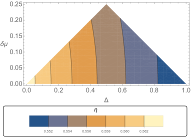
Figure 4: A contour plot to illustrate the effect of deficits and acceleration on uncharged nonrotating solutions. The efficiency is shown as a function of $\Delta$ and $\delta\mu$ for a cycle of unit radius centred at $(V_{0}=2,P_{0}=2)$.

Let us repeat our analysis to assess the effect of acceleration. Including non-zero $C$ in (28) yields

$$V =\frac{4S^{3/2}}{3\sqrt{\pi\Delta}}\frac{1+\left(\frac{3\Delta}{8PS}\right)^{2}\frac{2C^{2}}{(1+8PS/3\Delta)}}{\left[1-\left(\frac{3\Delta}{8PS}\right)\frac{4C^{2}}{(1+8PS/3\Delta)}\right]^{1/2}}$$ (31)

$$\approx\frac{4S^{3/2}}{3\sqrt{\pi\Delta}}\left[1+2\left(\frac{3\Delta C}{8PS}\right)^{2}\right]$$

upon expansion to order $C^{2}$. Note that since each tension $\mu_{\pm}$ is bounded by $1/4$, $\Delta C\leq 1/4$. Hence, unless we are dealing with very small black holes, this should be an excellent approximation. Inverting, we find

$$S =\left(\pi\Delta\right)^{\frac{1}{3}}\left(\frac{3V}{4}\right)^{\frac{2}{3}}\left[1-\frac{2C^{2}}{x_{0}^{2}}\right]^{\frac{1}{3}}$$ (32)

$$\Rightarrow\quad M =PV+\frac{\Delta^{\frac{2}{3}}}{2}\left(\frac{3V}{4\pi}\right)^{\frac{1}{3}}-\frac{\Delta^{2}C^{2}}{16\pi P^{2}V}\left(1+8\pi P\left(\frac{4V^{2}}{3\pi^{2}\Delta^{2}}\right)^{\frac{1}{3}}\right)\,,$$

where for shorthand we write

$$x_{0}=\frac{8PS}{3\Delta}\Bigg{|}_{C=0}=2P\left(\frac{4\pi V^{2}}{3\Delta^{2}}\right)^{\frac{1}{3}}\,.$$ (33)

Thus, the difference in mass across the cycle is

$$\Delta M=P_{0}\Delta V+\frac{\Delta^{\frac{2}{3}}}{2}\left(\frac{3}{4\pi}\right)^{\frac{1}{3}}(V_{1}^{\frac{1}{3}}-V_{2}^{\frac{1}{3}})+\frac{\Delta^{2}C^{2}}{16\pi P_{0}^{2}}\left(\frac{V_{1}-V_{2}}{V_{1}V_{2}}+6^{\frac{2}{3}}P_{0}\frac{4(V_{1}^{\frac{1}{3}}-V_{2}^{\frac{1}{3}})}{\Delta^{\frac{2}{3}}V_{1}^{\frac{1}{3}}V_{2}^{\frac{1}{3}}}\right)\,.$$ (34)

From (26) the effect of acceleration is to decrease efficiency, whereas the effect of a conical deficit is to increase it. This is illustrated in figure 4, and refines the findings of Zhang:2018vqs in which it was (incorrectly) reported that acceleration increases efficiency. Their conclusion followed from a choice of $K$ which regularised one of the C-metric’s poles. However, this constrains the thermodynamic charges and removes the independence of $\Delta$ and $C$. Our analysis shows that the situation is in fact more subtle. The dominant effect is the existence of the conical deficit, not the acceleration itself. When the thermodynamic charges are constrained by fixing $K$, these two effects are inseparable, giving a misleading picture of the phenomenology. This viewpoint is concurrent with the findings of Gregory:2019dtq in which it was argued that the average deficit is usually the more impactful of the two effects for the thermodynamics.

Figure 4 shows the efficiency contours in the $(\Delta,\delta\mu)$ plane for a circular benchmarking cycle of unit radius centred on $P_{0}=V_{0}=2$. The relatively small values of $P_{0}$ and $V_{0}$ (in contrast to the benchmarking cycles of Hennigar:2017apu ; Zhang:2018vqs ) were chosen to maximise the impact of acceleration. Even so, the contour lines are predominantly vertical, indicating that it is the value of $\Delta$, the mean deficit, that dominates the change in efficiency.

Once charges are added, the level of complexity rapidly rises, not least because the turning points from hot to cool parts of the cycle now arise at different $P$. As $Q$ or $J$ are increased, the points $\theta_{i}$ at which $\delta S$ vanishes are “shifted clockwise” around the cycle, in a qualitatively similar arrangement to the one shown in figure 3. We numerically explored this shifting, identifying $\theta_{i}$ for the complete range possible of cycle radii (those which kept pressure and volume positive) for a range of $P_{0}$ and $V_{0}$ from close to zero to values of order $10^{3}$, but were unable to identify valid choices of charges or deficits for which $\theta_{1}$ and $\theta_{2}$ did not fall in the upper–right and lower–left quadrants of the cycle respectively. This verifies that our efficiency formula (25) is valid across this broad sampling of the phase space for the metric (2).

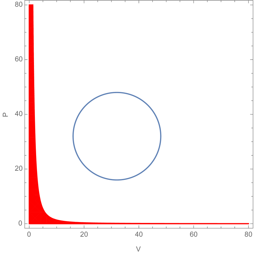
(a) $J=8$, $Q=0$, $\Delta=1$, $\delta\mu=0$.

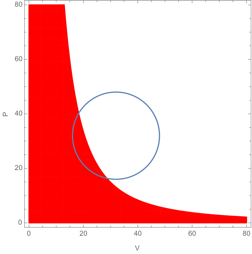
(b) $J=8$, $Q=0$, $\Delta=0.1$, $\delta\mu=0.01$.

Figure 5: An illustration of the truncation process. For the chosen value of charges and $\Delta$ and $\delta\mu$, the extremal limit template is plotted and the cycle superimposed. If it intersects the disallowed region, the grid point is removed from consideration. Here, in (a), the black hole without any deficit is allowed, whereas the grid point illustrated in (b) with acceleration and a deficit would be excluded.

Given this insight, we investigated the effect of acceleration on rotating and electrically charged black holes. We used both the method described in §3, and cross-checked against a discretised integration of the heat flow around the cycle – the method used in Hennigar:2017apu . First, the $(\Delta,\delta\mu)$ parameter space was discretised in a grid, and the cycle checked against a template for the chosen values of $Q$ and $J$, with the grid value of $\Delta$ and $\delta\mu$ to ensure that the cycle remains within the allowed region of parameter space with non-negative temperature (increasing $\Delta/C$ lowers the values of $Q$ and $J$ at which extremality occurs). Figure 5 illustrates this template procedure. Typically, charged cycles placed further from the origin in the $V$–$P$ plane can retain positive temperature over a larger range of $\Delta$, although the qualitative behaviour of efficiency remains the same.

Next, the efficiency was calculated at each point on the grid in the allowed region, and figures 6 and 7 illustrate the dependence of efficiency on the deficit and acceleration for sample values of $Q,J$ in benchmarking cycles closer to, and further from, the origin of the $(P,V)$ plane respectively.

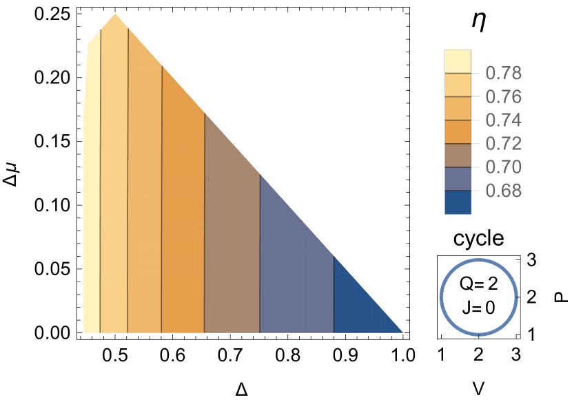
(a) Charged black hole, no rotation.

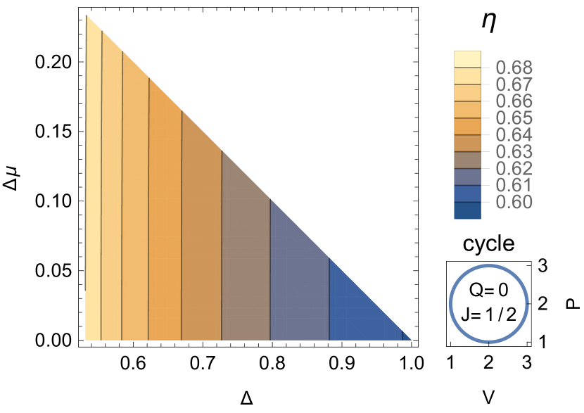
(b) Rotating black hole, no charge.

Figure 6: Contour plots of the efficiency dependence in the $(\Delta,\delta\mu)$ plane for a cycle centred on $P_{0}=V_{0}=2$ shown for a charged black hole in (a) and a rotating black hole in (b). Due to the placing of the cycle, and the chosen values of $J$ and $Q$, black holes on the cycle hit extremality for relatively large values of $\Delta$.

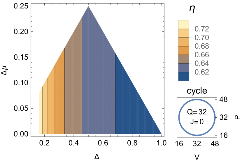
(a) Charged black hole, no rotation.

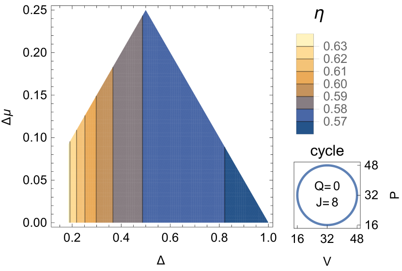
(b) Rotating black hole, no charge.

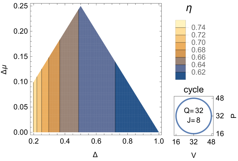
(c) Charged and rotating black hole.

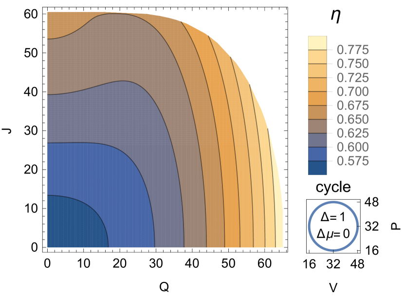
(d) The $Q$ and $J$ plane.

Figure 7: Contour plots of the efficiency dependence in the $(\Delta,\delta\mu)$ plane for a cycle centred on $P_{0}=V_{0}=32$ shown for black hole with either charge in (a), rotation in (b), or both in (c). In this case, the placing of the cycle allows a larger probe of the $(\Delta,\delta\mu)$ plane than figure 6. Subfigure (d) shows the dependence of efficiency on charge and rotation for the pure black hole for reference. The truncation of parameter space due to extremality is very clear.

It is clear from the figures that the general conclusion is that adding charge and rotation does not change the qualitative behaviour: the average conical deficit is dominant and acts to increase efficiency. If the geometry is restricted (as in Zhang:2018vqs ; Zhang:2018hms ) by imposing regularity on one axis, then as acceleration increases $\Delta$ will drop since the mean deficit is increasing, and the efficiency will increase. It is misleading to assign this effect to acceleration however, as figure 6 and 7 clearly show that significant changes in cycle efficiency are a consequence of the existence of a deficit, rather than the presence of acceleration.

5 Discussion

We have explored the impact of conical deficits on the efficiency of black hole heat engines. The result is that conical deficits give a marked improvement on the efficiency of black hole heat engines, whereas acceleration has a relatively small effect, and tends to decrease efficiency. In the literature, when considering an accelerating black hole, it is common to drive the acceleration by having a single cosmic string segment emerging from one pole of the black hole. By restricting the tension on the other pole to vanish, this leads to a constrained system - increasing acceleration necessarily increases the mean deficit of the spacetime, and it is this mean deficit that has the largest impact on thermodynamics.

A simple understanding of why conical deficits increase efficiency can be found by looking at the scaling (18). This shows how adding a deficit can be interpreted as a rescaling in the $(P,S)$ plane. The heat engines are cycles in the $(P,V)$ plane, and while in inverting $S(V,P,...)$ the other charges of the black hole come into play, there is no rescaling of these charges ($Q$, $J$) so that one can still map a cycle with $\Delta$ into a geometrically different cycle for the same black hole on the $(P,V)$ plane. Figure 8 gives a simple illustration of how the deficit can be thought of as a mapping between cycles on the $(P,V)$ plane for a rotating black hole (chosen because it has $C_{V}\neq 0$). The small square cycle near the origin is mapped to a larger distorted almost-parallelogram further from the origin. The efficiency of the square cycle for the $J=1$ black hole with $\Delta=0.75$ is mapped to the efficiency of the dashed cycle with $\Delta=1$. Given that larger black holes are closer to the ideal gas limit (and larger area cycles are typically more efficient), one can see the dual drivers towards greater efficiency in this mapping.

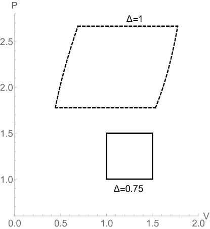
Figure 8: An illustration of the impact of a conical deficit on a square cycle of a rotating uncharged black hole ($J=1$).

A study of the efficiencies also reveals that the placing of the benchmarking cycle can impact on the details of how the efficiency varies. Typically, cycles placed closer to the origin have more variation with acceleration. This is understood from a study of the ‘vanilla’ C-metric as coming from the order of magnitude of the $C-$term. It is also interesting to note that rectangular benchmarking cycles bias against rotating black holes, as efficiency largely decreases with rotation, whereas circular cycles show a uniform increase. The efficiencies for each cycle are

$$\eta_{\text{circ}}=\frac{\pi R^{2}}{\Delta M-V_{0}\Delta P+{\cal S}/2+C_{1}}\;\;,\qquad\eta_{\text{rect}}=\frac{A}{\Delta M-V_{L}\Delta P}$$ (35)

where $\Delta M$ is the mass difference across the turning points of the cycle, that typically increases with $J$ at fixed points in the $(P,V)$ plane. $\Delta P$ likewise is the pressure difference, however, this has a very different meaning for the rectangular and circular cycles. For the rectangular cycle, the turning points are fixed, so the only variation is in $\Delta M$ in the denominator that increases as $J$ increases, thus the efficiency drops. For the circular cycle however, the turning points shift as rotation is increased, so, not only is the contribution from the geometric terms on the denominator lowered, but also the masses at the turning points, and $\Delta M$, (although this is less obvious to see) hence efficiency increases. This was precisely the motivation of Chakraborty and Johnson to consider more general cycles in the $(P,V)$ plane Chakraborty:2016ssb ; Chakraborty:2017weq .

Figure 9: The exclusion region for a vanilla accelerating black hole.

Finally, although we did not explore extremely close to the origin of the $(P,V)$ plane, there are additional “no-go” regions once acceleration is introduced (see fig. 9). For small nonrotating black holes, it is possible for the enthalpy to vanish due to the exothermic effect of acceleration in (16). This then means that the thermodynamic volume has a minimum, leading to an exclusion region very near the origin. This is related to the “snapping swallowtail” phenomenon noted in Abbasvandi:2018vsh ; Gregory:2019dtq ; Abbasvandi:2019vfz . Thus, even though acceleration has little impact on the black hole heat engine efficiency, it introduces some new subtleties for the phase plane of the holographic heat engine.

- (1) J. M. Maldacena, The Large N limit of superconformal field theories and supergravity, Int. J. Theor. Phys. 38 (1999) 1113 [Adv. Theor. Math. Phys. 2 (1998) 231] [hep-th/9711200].
- (2) S. S. Gubser, I. R. Klebanov and A. M. Polyakov, Phys. Lett. B 428, 105 (1998) doi:10.1016/S0370-2693(98)00377-3 [hep-th/9802109].
- (3) E. Witten, Anti-de Sitter space and holography, Adv. Theor. Math. Phys. 2, 253 (1998) [hep-th/9802150].
- (4) A. Chamblin, R. Emparan, C. V. Johnson and R. C. Myers, Charged AdS black holes and catastrophic holography, Phys. Rev. D 60, 064018 (1999) [hep-th/9902170].
- (5) D. Z. Freedman, S. S. Gubser, K. Pilch and N. P. Warner, Renormalization group flows from holography supersymmetry and a c theorem, Adv. Theor. Math. Phys. 3, 363 (1999) [hep-th/9904017].
- (6) M. M. Caldarelli, G. Cognola and D. Klemm, Thermodynamics of Kerr-Newman-AdS black holes and conformal field theories, Class. Quant. Grav. 17, 399 (2000) [hep-th/9908022].
- (7) R. C. Myers and A. Sinha, Seeing a c-theorem with holography, Phys. Rev. D 82 (2010) 046006 [arXiv:1006.1263 [hep-th]].
- (8) S. W. Hawking and D. N. Page, Thermodynamics of Black Holes in anti-De Sitter Space, Commun. Math. Phys. 87, 577 (1983).
- (9) H. Casini, M. Huerta and R. C. Myers, Towards a derivation of holographic entanglement entropy, JHEP 1105 (2011) 036 [arXiv:1102.0440 [hep-th]].
- (10) C. V. Johnson and F. Rosso, Holographic Heat Engines, Entanglement Entropy, and Renormalization Group Flow, Class. Quant. Grav. 36 (2019) no.1, 015019 [arXiv:1806.05170 [hep-th]].
- (11) D. Kubizňák, R. B. Mann and M. Teo, Black hole chemistry: thermodynamics with Lambda, Class. Quant. Grav. 34, no. 6, 063001 (2017) [arXiv:1608.06147 [hep-th]].
- (12) M. Henneaux and C. Teitelboim, The Cosmological Constant As A Canonical Variable, Phys. Lett. 143B, 415 (1984).
- (13) C. Teitelboim, The Cosmological Constant As A Thermodynamic Black Hole Parameter, Phys. Lett. 158B, 293 (1985).
- (14) D. Kastor, S. Ray and J. Traschen, Enthalpy and the Mechanics of AdS Black Holes, Class. Quant. Grav. 26, 195011 (2009) [arXiv:0904.2765 [hep-th]].
- (15) B. P. Dolan, The cosmological constant and the black hole equation of state, Class. Quant. Grav. 28, 125020 (2011) [arXiv:1008.5023 [gr-qc]].
- (16) B. P. Dolan, Pressure and volume in the first law of black hole thermodynamics, Class. Quant. Grav. 28, 235017 (2011) [arXiv:1106.6260 [gr-qc]].
- (17) D. Kubizňák and R. B. Mann, P-V criticality of charged AdS black holes, JHEP 1207, 033 (2012) [arXiv:1205.0559 [hep-th]].
- (18) B. P. Dolan, Where Is the PdV in the First Law of Black Hole Thermodynamics?, [arXiv:1209.1272 [gr-qc]].
- (19) M. Cvetic, G. W. Gibbons, D. Kubizňák and C. N. Pope, Black Hole Enthalpy and an Entropy Inequality for the Thermodynamic Volume, Phys. Rev. D 84, 024037 (2011) [arXiv:1012.2888 [hep-th]].
- (20) B. P. Dolan, D. Kastor, D. Kubizňák, R. B. Mann and J. Traschen, Thermodynamic Volumes and Isoperimetric Inequalities for de Sitter Black Holes, Phys. Rev. D 87, no. 10, 104017 (2013) [arXiv:1301.5926 [hep-th]].
- (21) R. Gregory and A. Scoins, Accelerating Black Hole Chemistry [arXiv:1904.09660 [hep-th]].
- (22) N. Altamirano, D. Kubizňák, R. B. Mann and Z. Sherkatghanad, Kerr-AdS analogue of triple point and solid/liquid/gas phase transition, Class. Quant. Grav. 31 (2014) 042001 [arXiv:1308.2672 [hep-th]].
- (23) S. Gunasekaran, R. B. Mann and D. Kubizňák, Extended phase space thermodynamics for charged and rotating black holes and Born-Infeld vacuum polarization, JHEP 1211 (2012) 110 [arXiv:1208.6251 [hep-th]].
- (24) R. A. Hennigar, R. B. Mann and E. Tjoa, Superfluid Black Holes, Phys. Rev. Lett. 118 (2017) no.2, 021301 [arXiv:1609.02564 [hep-th]].
- (25) D. Kastor, S. Ray and J. Traschen, Chemical Potential in the First Law for Holographic Entanglement Entropy, JHEP 1411 (2014) 120 [arXiv:1409.3521 [hep-th]].
- (26) B. P. Dolan, Bose condensation and branes, JHEP 1410 (2014) 179 [arXiv:1406.7267 [hep-th]].
- (27) A. Karch and B. Robinson, Holographic Black Hole Chemistry, JHEP 1512 (2015) 073 [arXiv:1510.02472 [hep-th]].
- (28) C. V. Johnson, Holographic Heat Engines, Class. Quant. Grav. 31 (2014) 205002 [arXiv:1404.5982 [hep-th]].
- (29) C. V. Johnson, An Exact Efficiency Formula for Holographic Heat Engines, Entropy 18 (2016) 120 [arXiv:1602.02838 [hep-th]].
- (30) F. Rosso, Holographic heat engines and static black holes: a general efficiency formula, Int. J. Mod. Phys. D 28 (2018) no.02, 1950030 [arXiv:1801.07425 [hep-th]].
- (31) A. Chakraborty and C. V. Johnson, Benchmarking black hole heat engines, I, Int. J. Mod. Phys. D 27 (2018) no.16, 1950012 [arXiv:1612.09272 [hep-th]].
- (32) A. Chakraborty and C. V. Johnson, Benchmarking Black Hole Heat Engines, II, Int. J. Mod. Phys. D 27 (2018) no.16, 1950006 [arXiv:1709.00088 [hep-th]].
- (33) C. V. Johnson, Holographic Heat Engines as Quantum Heat Engines, [arXiv:1905.09399 [hep-th]].
- (34) R. A. Hennigar, F. McCarthy, A. Ballon and R. B. Mann, Holographic heat engines: general considerations and rotating black holes, Class. Quant. Grav. 34 (2017) no.17, 175005 [arXiv:1704.02314 [hep-th]].
- (35) J. Zhang, Y. Li and H. Yu, Accelerating AdS black holes as the holographic heat engines in a benchmarking scheme, Eur. Phys. J. C 78 (2018) no.8, 645 [arXiv:1801.06811 [hep-th]].
- (36) J. Zhang, Y. Li and H. Yu, Thermodynamics of charged accelerating AdS black holes and holographic heat engines, JHEP 1902, 144 (2019) doi:10.1007/JHEP02(2019)144 [arXiv:1808.10299 [hep-th]].
- (37) A. Anabalón, M. Appels, R. Gregory, D. Kubizňák, R. B. Mann and A. Övgün, Holographic Thermodynamics of Accelerating Black Holes, [arXiv:1805.02687 [hep-th]].
- (38) A. Anabalón, F. Gray, R. Gregory, D. Kubizňák and R. B. Mann, Thermodynamics of Charged, Rotating, and Accelerating Black Holes, [arXiv:1811.04936 [hep-th]].
- (39) M. Appels, R. Gregory and D. Kubizňák, Thermodynamics of Accelerating Black Holes, Phys. Rev. Lett. 117, no. 13, 131303 (2016) [arXiv:1604.08812 [hep-th]].
- (40) M. Appels, R. Gregory and D. Kubizňák, Black Hole Thermodynamics with Conical Defects, JHEP 1705, 116 (2017) [arXiv:1702.00490 [hep-th]].
- (41) R. Gregory, Accelerating Black Holes, J. Phys. Conf. Ser. 942, no. 1, 012002 (2017) [arXiv:1712.04992 [hep-th]].
- (42) M. Astorino, CFT Duals for Accelerating Black Holes, Phys. Lett. B 760, 393 (2016) [arXiv:1605.06131 [hep-th]].
- (43) M. Astorino, Thermodynamics of Regular Accelerating Black Holes, [arXiv:1612.04387 [gr-qc]].
- (44) M. Appels, Thermodynamics of Accelerating Black Holes, Ph.D. thesis, Durham U., Dept. of Math., 2018.
- (45) K. Dutta, S. Ray and J. Traschen, Boost mass and the mechanics of accelerated black holes, Class. Quant. Grav. 23, 335 (2006) [hep-th/0508041].
- (46) W. Kinnersley and M. Walker, Uniformly accelerating charged mass in general relativity, Phys. Rev. D 2, 1359 (1970).
- (47) J. F. Plebanski and M. Demianski, Rotating, charged, and uniformly accelerating mass in general relativity, Annals Phys. 98, 98 (1976).
- (48) J. B. Griffiths and J. Podolsky, A New look at the Plebanski-Demianski family of solutions, Int. J. Mod. Phys. D 15 (2006) 335 [gr-qc/0511091].
- (49) M. Aryal, L. Ford, and A. Vilenkin, Cosmic strings and black holes, Phys.Rev. D34 (1986) 2263.
- (50) A. Achucarro, R. Gregory, and K. Kuijken, Abelian Higgs hair for black holes, Phys.Rev. D52 (1995) 5729–5742, [gr-qc/9505039].
- (51) R. Gregory and M. Hindmarsh, Smooth metrics for snapping strings, Phys. Rev. D 52, 5598 (1995) [gr-qc/9506054].
- (52) R. Gregory, D. Kubizňák and D. Wills, Rotating black hole hair, JHEP 1306, 023 (2013) [arXiv:1303.0519 [gr-qc]].
- (53) R. Gregory, P. C. Gustainis, D. Kubizňák, R. B. Mann and D. Wills, Vortex hair on AdS black holes, JHEP 1411, 010 (2014) [arXiv:1405.6507 [hep-th]].
- (54) J. Podolsky, Accelerating black holes in anti-de Sitter universe, Czech. J. Phys. 52, 1 (2002) [gr-qc/0202033].
- (55) L. Smarr, Mass formula for Kerr black holes, Phys. Rev. Lett. 30, 71 (1973) Erratum: [Phys. Rev. Lett. 30, 521 (1973)].
- (56) N. Abbasvandi, W. Cong, D. Kubizňák and R. B. Mann, Snapping swallowtails in accelerating black hole thermodynamics, [arXiv:1812.00384 [gr-qc]].
- (57) N. Abbasvandi, W. Ahmed, W. Cong, D. Kubizňák and R. B. Mann, Finely Split Phase Transitions of Rotating and Accelerating Black Holes, [arXiv:1906.03379 [gr-qc]].
- (58) D. Christodoulou and R. Ruffini, Reversible transformations of a charged black hole, Phys. Rev. D 4, 3552 (1971).