On the Erdős–Sós conjecture for trees with bounded degree

Abstract

We prove the Erdős–Sós conjecture for trees with bounded maximum degree and large dense host graphs. As a corollary, we obtain an upper bound on the multicolour Ramsey number of large trees whose maximum degree is bounded by a constant.

1 Introduction

Given $k\in\mathbb{N}$, the famous Erdős–Sós conjecture from 1964 (see [4]) states that every graph with average degree greater than $k-1$ contains all trees with $k$ edges. This conjecture is tight for every $k\in\mathbb{N}$, which can be seen by considering the complete graph on $k$ vertices. This graph has average degree $k-1$ but it is too small to contain any tree with $k$ edges. A structurally different example is the balanced complete bipartite graph on $2k-2$ vertices (where by balanced we mean that the bipartition classes have equal sizes). This graph has average degree $k-1$ but does not contain the $k$-edge star. In order to obtain examples of larger order, one can consider the disjoint union of copies of the two extremal graphs we just described.

It is easy to see that the Erdős–Sós conjecture is true for stars and double stars (the latter are graphs obtained by joining the centres of two stars with an edge). A classical result of Erdős and Gallai [5] implies that it also holds for paths. In the early 90’s Ajtai, Komlós, Simonovits and Szemerédi announced a proof of the Erdős–Sós conjecture for large $k$. Nevertheless, many particular cases has been settled since then. For instance, Brandt and Dobson [3] proved that the Erdős–Sós conjecture is true for graphs with girth at least $5$, and Saclé and Woźniak [15] proved it for $C_{4}$-free graphs. Goerlich and Zak [7] proved the Erdős–Sós conjecture for graphs of order $n=k+c$, where $c$ is a given constant and $k$ is sufficiently large depending on $c$. More recently, Rozhoň [14] gave an approximate version of the Erdős–Sós conjecture for trees with linearly bounded maximum degree and dense host graph. Independently, the authors proved in [2] a similar result but for trees with maximum degree bounded by $k^{\frac{1}{67}}$ and dense host graphs.

Given a positive integers $k$ and $\Delta$, let $\mathcal{T}(k,\Delta)$ denote the set of all trees $T$ with $k$ edges and $\Delta(T)\leq\Delta$. The main result of this paper is that the Erdős–Sós conjecture holds for all trees whose maximum degree is bounded by a constant and whose size is linear in the order of the host graph.

Theorem 1.1.

For all $\delta>0$ and $\Delta\in\mathbb{N}$, there is $n_{0}\in{\mathbb{N}}$ such that for each $k,n\in\mathbb{N}$ with $n\geq n_{0}$ and $n\geq k\geq\delta n$, and for each $n$-vertex graph $G$ the following holds. If $G$ satisfies $d(G)>k-1$, then $G$ contains every tree $T\in\mathcal{T}(k,\Delta)$.

Our proof of Theorem 1.1 splits into two cases. If $G$ is connected and considerably larger than $k$, we proceed as follows. After regularising $G$ we inspect the components of the reduced graph, at least one of which has to have large average degree. If this component is large enough, then we can show it is either bipartite or contains a useful matching structure, and can embed any given tree $T\in\mathcal{T}(k,\Delta)$ using regularity and tools from [2]. Otherwise, the reduced graph is a union of graphs corresponding to the description given in the first paragraph of the Introduction, that is, graphs which are almost complete and of size roughly $k$ or balanced almost complete bipartite graphs of size roughly $2k$. In that case we use an edge of $G$ to connect two components and embed $T$ there.

If, on the other hand, the order of the host graph is very close to $k$, if the host graph is close to being a bipartite graph of order $2k$, or if the host graph is the disjoint union of such graphs, then a different approach is needed. To take care of these cases, we prove the following result, Theorem 1.2.

This theorem might be of independent interest as it greatly improves the main result from [7] for bounded degree trees. Note that given a graph $G$ with $d(G)>k-1$, a standard argument shows that $G$ has a subgraph of minimum degree $\delta(G)\geq\frac{k}{2}$ that preserves the average degree. So, since in the Erdős-Sós conjecture and all our theorems, we are looking for subgraphs, we may always assume that in addition to the average degree condition, $G$ fulfills a minimum degree condition. (In particular, this is assumed in Theorem 1.2.)

Given $\beta>0$, we say that a graph $H$ is $\beta$-bipartite if there is a partition $V(H)=A\cup B$ such that $e(A)+e(B)\leq\beta e(H).$

Theorem 1.2.

For each $k,\Delta\in\mathbb{N}$ and each graph $G$ with $d(G)>k-1$ and $\delta(G)\geq\frac{k}{2}$ the following holds.

1. If $k\geq 10^{6}$ and $|G|\leq(1+10^{-11})k$ then $G$ contains each tree $T\in\mathcal{T}(k,\frac{\sqrt{k}}{1000})$.

2. If $k\geq 8\Delta^{2}$ and $G=(A,B)$ is $\frac{1}{50\Delta^{2}}$-bipartite with $|A|,|B|\leq(1+\frac{1}{25\Delta^{2}})k$ then $G$ contains each tree $T\in\mathcal{T}(k,\Delta)$.

As a third result we prove an approximate version of the Erdős–Sós conjecture for trees with linearly bounded maximum degree and dense host graph; this was independently proved by Rozhoň [14].

Theorem 1.3.

For all $\delta\in(0,1)$ there are $n_{0}\in{\mathbb{N}}$ and $\gamma\in(0,1)$ such that for each $k$ and for each $n$-vertex graph $G$ with $n\geq n_{0}$ and $n\geq k\geq\delta n$ the following holds. If $G$ satisfies $d(G)\geq(1+\delta)k$, then $G$ contains every tree $T\in\mathcal{T}(k,\gamma k)$.

Finally, let us briefly mention a well-known consequence of the Erdős–Sós conjecture in Ramsey theory. Given an integer $\ell\geq 2$ and a graph $H$, the $\ell$-colour Ramsey number $r_{\ell}(H)$ of $H$ is the smallest $n\in\mathbb{N}$ such that every $\ell$-colouring of the edges of $K_{n}$ yields a monochromatic copy of $H$. In 1973, Erdős and Graham conjectured [6] that every tree $T$ with $k$ edges satisfies

$$r_{\ell}(T)=\ell(k+1)+O(1),$$ (1)

and they established the lower bound $r_{\ell}(T)>\ell(k+1)+1$ for large enough $\ell$ satisfying $\ell\equiv 1\mod k$. Erdős and Graham also observed that the upper bound in (1) would follow from the Erdős–Sós conjecture. Indeed, for $n\geq\ell(k-1)+2$ note that the most popular colour in any $\ell$-colouring of $K_{n}$ has at least $\frac{1}{\ell}\binom{n}{2}$ edges and thus average degree at least $\frac{n-1}{\ell}>k-1$. So the Erdős–Sós conjecture would imply that the most popular colour contains a copy of every tree with $k$ edges. Therefore, from Theorem 1.1 we deduce the following result.

Corollary 1.4.

For all $\ell\geq 2$, $\Delta\in\mathbb{N}$ there exists $k_{0}\in\mathbb{N}$ such that for every $k\geq k_{0}$ and every tree $T\in\mathcal{T}(k,\Delta)$ we have $r_{\ell}(T)\leq\ell(k-1)+2.$

We remark that in Corollary 1.4 one can actually find a copy of every tree $T\in\mathcal{T}(k,\Delta)$ in the same colour, at the same time.

The paper is organised as follows. After some preliminaries in Section 2, we prove Theorem 1.1 in Section 3. That Section also contains the proof of Theorem 1.2, more precisely, Theorem 1.2 follows directly from Propositions 3.1 and 3.3 stated and proved in that section. We finally prove Theorem 1.3 in Section 4.

2 Preliminaries

2.1 Notation

For $\ell\in\mathbb{N}$, we write $[\ell]$ for the discrete interval $\{1,\ldots,\ell\}$. We write $a\ll b$ to indicate that given a constant $b$, constant $a$ is chosen significantly smaller. The explicit value for such $a$ can be calculated from the proofs. Also, we write $a=b\pm c$ if $a\in[b-c,b+c]$.

Given a graph $H$, write $|H|=|V(H)|$ and $e(H)=|E(H)|$. Let $\delta(H)$, $d(H)$ and $\Delta(H)$ denote the minimum, average and maximum degree of $H$, respectively. As usual, $\deg_{H}(x)$ denotes the degree of a vertex $x\in V(H)$, and we write $N_{H}(x)$ for its neighbourhood in $H$, $N_{H}(x,S)=N_{H}(x)\cap S$ for its neighbourhood in $S\subseteq V(H)$ and $\deg_{H}(x,S)$ for the respective degree. For two sets $X,Y\subseteq V(H)$, we write $E_{H}(X,Y)$ for the family of edges $xy\in E(H)$ with $x\in X$ and $y\in Y$ and set $e_{H}(X,Y):=|E_{H}(X,Y)|$. Note that edges lying in the intersection of $X$ and $Y$ are counted twice. In all of the above, we omit the subscript $H$ if it is clear from the context. Given $U\subset V(H)$ we write $H[U]$ for the graph induced in $H$ by the vertices in $U$, and we say a vertex $x$ sees $U$ if it has at least one neighbour in $U$.

Given a collection of sets $\mathcal{F}$, we write $\bigcup\mathcal{F}$ for the union of all members of $\mathcal{F}$. If $\mathcal{G}$ is a collection of graphs, then $\bigcup\mathcal{G}$ denotes the graph which is the union of all graphs in $\mathcal{G}$.

2.2 Regularity Lemma

Let us fix two parameters $\varepsilon,\eta\in(0,1)$. Let $H=(A,B;E)$ be a bipartite graph with density $d(A,B):=\frac{e(A,B)}{|A||B|}$. We say that the pair $(A,B)$ is $\varepsilon$-regular if

$$|d(X,Y)-d(A,B)|<\varepsilon$$

for all $X\subseteq A$ and $Y\subseteq B$, with $|X|>\varepsilon|A|$ and $|Y|>\varepsilon|B|$. Furthermore, we say that $(A,B)$ is $(\varepsilon,\eta)$-regular if $(A,B)$ is $\varepsilon$-regular and $d(A,B)\geq\eta$. Given an $\varepsilon$-regular pair $(A,B)$, with density $d$, we say that a subset $X\subseteq A$ is $\varepsilon$-significant if $|X|>\varepsilon|A|$ (analogously for subsets of $B$). A vertex $x\in A$ is called $\varepsilon$-typical to a significant set $Y\subseteq B$ if $\deg(x,Y)>(d-\varepsilon)|Y|$, and similar for a vertex $x\in B$. We will write just regular, significant or typical if $\varepsilon$ is clear from the context.

Regular pairs behave like a typical random graph of the same edge density. For instance, almost every vertex is typical to any given significant set, and regularity is inherited by subpairs. Let us state these well-known facts in a precise form (see [10] for a proof).

Fact 2.1.

Let $(A,B)$ be an $\varepsilon$-regular pair with density $d$. Then the following holds:

1. For any $\varepsilon$-significant $Y\subseteq B$, all but at most $\varepsilon|A|$ vertices from $A$ are $\varepsilon$-typical to $Y$.

2. Let $\alpha\in(0,1)$. For any subsets $X\subseteq A$ and $Y\subseteq B$, with $|X|\geq\alpha|A|$ and $|Y|\geq\alpha|B|$, the pair $(X,Y)$ is $\frac{2\varepsilon}{\alpha}$-regular with density $d\pm\varepsilon$.

Given a graph $G$, we say that a vertex partition $V(G)=V_{1}\cup\ldots\cup V_{\ell}$ is $(\varepsilon,\eta)$-regular if

1. $|V_{1}|=|V_{2}|=\ldots=|V_{\ell}|$;

2. $V_{i}$ is independent for all $i\in[\ell]$; and

3. for all $1\leq i<j\leq\ell$, the pair $(V_{i},V_{j})$ is $\varepsilon$-regular with density either $d(V_{i},V_{j})\geq\eta$ or $d(V_{i},V_{j})=0$.

Szemerédi’s regularity lemma [16] states that every large graph has an almost spanning subgraph that admits a regular partition. We will use the following version (see for instance [10]).

Lemma 2.2 (Regularity lemma).

For all $\varepsilon>0$ and $m_{0}\in{\mathbb{N}}$ there are $N_{0},M_{0}$ such that the following holds for all $\eta\in[0,1]$ and $n\geq N_{0}$. Any $n$-vertex graph $G$ has a subgraph $G^{\prime}$, with $|G|-|G^{\prime}|\leq\varepsilon n$ and $\deg_{G^{\prime}}(x)\geq\deg_{G}(x)-(\eta+\varepsilon)n$ for all $x\in V(G^{\prime})$, such that $G^{\prime}$ admits an $(\varepsilon,\eta)$-regular partition $V(G^{\prime})=V_{1}\cup\ldots\cup V_{\ell}$, with $m_{0}\leq\ell\leq M_{0}$.

The $(\varepsilon,\eta)$-reduced graph $\mathscr{R}$ corresponding to the $(\varepsilon,\eta)$-regular partition that is given by Lemma 2.2 has vertex set $V(\mathscr{R})=\{V_{i}:i\in[\ell]\}$, called clusters, and an edge $V_{i}V_{j}$ for each $i,j$ with $d(V_{i},V_{j})\geq\eta$. We use calligraphic letters to refer to the reduced graph, or to subsets of its vertex set. Moreover, given $\mathscr{C}\subseteq V(\mathscr{R})$, we write $|\mathscr{C}|$ for the number of clusters in $\mathscr{C}$. In contrast, we write $|\bigcup\mathscr{C}|$ for the number of vertices of the subgraph $\bigcup\mathscr{C}$ of $G$. Now we state some useful facts about the reduced graph (see [10] for a proof).

Fact 2.3.

Let $G$ be a $n$-vertex graph and let $\mathscr{R}$ be an $(\varepsilon,\eta)$-reduced graph of $G$. Then the following holds.

1. Given a cluster $C\in V(\mathscr{R})$ we have

   $$\deg_{\mathscr{R}}(C)\geq\frac{1}{|C|}\sum_{v\in C}\deg(v)\cdot\frac{|\mathscr{R}|}{n}.$$

   In particular, summing over all clusters we have $d(\mathscr{R})\geq d(G)\cdot\frac{|\mathscr{R}|}{n}$.

2. Let $\mathscr{Y}$ be a collection of significant sets of clusters in $\mathscr{R}$ and let $C\in V(\mathscr{R})$. Then

   $$|\{Y\in\mathscr{Y}:v\text{ is typical to }Y\}|\geq(1-\sqrt{\varepsilon})|\mathscr{Y}|$$

   for all but at most $\sqrt{\varepsilon}|C|$ vertices $v\in C$.

We close this subsection with a well-known lemma that illustrates why regularity is so useful for embedding trees. It states that a tree will always fit into a regular pair, if the tree is small enough (but it may still be linear in the size of the pair). A proof can be found for instance in [1, 2].

Lemma 2.4.

Let $0<\beta\leq\varepsilon\leq\tfrac{1}{25}$. Let $(A,B)$ be a $(\varepsilon,5\sqrt{\varepsilon})$-regular pair with $|A|=|B|=m$, and let $X\subseteq A,Y\subseteq B,Z\subseteq A\cup B$ be such that $\min\{|X\setminus Z|,|Y\setminus Z|\}>\sqrt{\varepsilon}m$.
Then any tree $T$ on at most $\beta m$ vertices can be embedded into $(X\cup Y)\setminus Z$. Moreover, for each $v\in V(T)$ there are at least $2\varepsilon m$ vertices from $(X\cup Y)\setminus Z$ that can be chosen as the image of $v$.

2.3 Trees

Let us give some notation for trees. We will write $(T,r)$ for a tree $T$ rooted at $r\in V(T)$. Given any rooted tree $(T,r)$ and $x,y\in V(T)$, we say that $x$ is below $y$ (resp. $y$ is above $x$) if $y$ lies on the unique path from $x$ to $r$ (our trees grow from the top to the bottom). If in addition, $xy\in E(T)$, we say $x$ is a child of $y$, and $y$ is the parent of $x$.

The following lemma allow us to find a cut vertex which splits the tree into connected components of convenient sizes. See [2, 8, 13] for other variants and a proof.

Lemma 2.5.

For all $0<\gamma\leq 1$ and for all $k\geq\frac{200}{\gamma}$, any given tree $T$ with $k$ edges has a subtree $(T^{*},t^{*})$ such that

1. $\frac{\gamma k}{2}\leq|V(T^{*})|\leq\gamma k$; and

2. every component of $T-T^{*}$ is adjacent to $t^{*}$.

A bare path in a tree is a path all whose internal vertices have degree $2$ in the tree. The next lemma has been extensively used in the literature of tree embeddings. It states that the structure of any given tree satisfies a certain dichotomy. Namely, each tree contains either a large number of leaves or a large number of bare paths of some fixed constant length (we refer to [11, 12] for a more general statement and a proof, and note that here, the length of a path is its number of edges).

Lemma 2.6.

Let $\ell>2$ and let $T$ be a tree. Then either $T$ has at least $|T|/4\ell$ leaves or it has at least $|T|/4\ell$ vertex disjoint bare paths, each of length $\ell$.

Another well-known fact we shall use in our proof is the following. One can prove it by rooting the tree at any vertex in the smaller bipartition class, and comparing the number of vertices in a odd level to the number of vertices in the preceding level.

Fact 2.7.

Let $T$ be a tree with bipartition $V(T)=C\cup D$ and maximum degree $\Delta(T)\leq\Delta$. Then $\min\{|C|,|D|\}\geq\frac{k}{\Delta}.$

2.4 Tree embeddings

A greedy argument shows that every $k$-edge tree can be embedded into any graph of minimum degree at least $k$. We give two lemmas that generalise this simple observation.

Lemma 2.8.

Let $\Delta,h,k\in{\mathbb{N}}$, let $(T,r)$ be a tree with $k-h$ edges and $\Delta(T)\leq\Delta$, and let $G$ be a graph satisfying

1. $\delta(G)\geq\Delta+h$;

2. there are at most $h$ vertices $x\in V(G)$ with $\deg(x)<k$.

Then $T$ can be embedded in $G$. Moreover, any vertex $v$ of $G$ can be chosen as the image of $r$.

Proof.

We construct an embedding $\phi$ as follows. We set $\phi(r):=v$. Since $\deg(v)\geq\Delta+h$, we can embed each neighbour of $r$ into a neighbour of $v$ that has degree at least $k$. Since $T$ has $k-h$ vertices, we can then embed the rest of $T$ levelwise using only vertices of degree at least $k$ at each step. ∎

Observe that for $h=0$ Lemma 2.8 recovers the greedy procedure we mentioned above.

If the host graph $G$ is bipartite, one can relax the minimum degree condition for one side of the bipartition of $G$. We leave the proof of the following lemma to the reader.

Lemma 2.9.

Let $\Delta,h,k_{1},k_{2}\in{\mathbb{N}}$, let $(T,r)$ be a tree with colour classes $C,D$ of sizes $k_{1}-h$ and $k_{2}-h$, respectively, and $\Delta(T)\leq\Delta$. Let $G=(A,B)$ be a bipartite graph such that

1. $\delta(G)\geq\Delta+h$;

2. there are at most $h$ vertices $a\in A$ with $\deg(x)<k_{2}$;

3. there are at most $h$ vertices $b\in B$ with $\deg(x)<k_{1}$.

Then $T$ can be embedded into $G$ with $C$ going to $A$ and $D$ going to $B$. Moreover, if $r\in C$ (resp. $D$), then any vertex $a\in A$ (resp. $b\in B$) can be chosen as the image of $r$.

2.5 Matching lemma

Later on we will need the following lemma on matchings in graphs with large minimum degree. This lemma is a slight variation of Lemma 5.7 from [2].

Lemma 2.10.

Let $\varepsilon,\eta\in(0,1)$, let $t,\ell\in\mathbb{N}$, and let $G$ be a graph on $n\geq 2t+\ell$ vertices with $\delta(G)\geq t+\ell$ which has an $(\varepsilon,\eta)$-regular partition into $\ell$ parts. Then $G$ has a subgraph $G^{\prime}$ with $|G^{\prime}|\geq n-\ell$ that admits a $(5\varepsilon,\eta-\varepsilon)$-regular partition with $2\ell$ parts whose corresponding reduced graph $\mathscr{R}$ contains a matching $\mathscr{M}$ and an independent family of clusters $\mathscr{I}$, disjoint from $\mathscr{M}$, such that

1. $\bigcup V(\mathscr{M})\cup V(\bigcup\mathscr{I})=V(G^{\prime})$;

2. $|\bigcup V(\mathscr{M})|\geq 2t$; and

3. there is a partition $V(\mathscr{M})=\mathscr{V}_{1}\cup\mathscr{V}_{2}$ such that $N_{\mathscr{R}}(\mathscr{I})\subseteq\mathscr{V}_{1}$ and every edge in $\mathscr{M}$ has one endpoint in $\mathscr{V}_{1}$ and one endpoint in $\mathscr{V}_{2}$.

3 Trees with constant maximum degree

In this section we work towards the proof of our main result, Theorem 1.1, and along the way, we prove Theorem 1.2. This latter theorem follows directly from Propositions 3.1 and 3.3. These are proved in Sections 3.1 and 3.2, respectively. In Section 3.3 we use a regularity approach and results from [2] to cover the case when the host graph is significantly larger than the tree. Finally, in Subsection 3.4, we put everything together to prove Theorem 1.1.

3.1 Almost complete bipartite graphs

Recall that $H$ is $\beta$-bipartite if at least a $(1-\beta)$-fraction of its edges lie between $A$ and $B$.

Proposition 3.1.

Let $k,\Delta\in\mathbb{N}$ such that $k\geq 8\Delta^{2}$. Let $G=(A,B)$ be a $\frac{1}{50\Delta^{2}}$-bipartite graph, with $|A|,|B|\leq(1+\frac{1}{25\Delta^{2}})k$, $d(G)>k-1$ and $\delta(G)\geq\frac{k}{2}$. Then $G$ contains each tree $T\in\mathcal{T}(k,\Delta)$.

Proof.

Set $\varepsilon:=\frac{1}{25\Delta^{2}}$ and write $n=|V(G)|$. Then, $n\leq(1+\varepsilon)2k$. Since $G$ is $\frac{\varepsilon}{2}$-bipartite, we know that $e(A,B)\geq(1-\varepsilon)\frac{kn}{2}.$ Suppose that $|B|\geq\frac{n}{2}\geq|A|$. Then

$$\frac{1}{|A|}\sum_{a\in A}\deg(a,B)>\frac{(1-\varepsilon)kn}{2|A|}\geq(1-\varepsilon)k,$$ (2)

and thus $|B|\geq(1-\varepsilon)k$. Furthermore, since $n=|A|+|B|$, we have

$$|A||B|\geq e(A,B)\geq(1-\varepsilon)\frac{kn}{2}\geq(1-\varepsilon)k\sqrt{|A||B|},$$

and thus, the fact that $|B|\leq(1+\varepsilon)k$ implies that $|A|\geq\frac{(1-\varepsilon)^{2}}{1+\varepsilon}k\geq(1-3\varepsilon)k.$ Now we can give a lower bound for the average degree from $B$ to $A$ by using the first inequality from (2) and the fact that $n=|A|+|B|$ to calculate

$$\frac{1}{|B|}\sum_{b\in B}\deg(b,A)>(1-\varepsilon)\frac{k}{2}\Big{(}1+\frac{|A|}{|B|}\Big{)}\geq\frac{1-\varepsilon}{2}\Big{(}1+\frac{1-3\varepsilon}{1+\varepsilon}\Big{)}k\geq(1-4\varepsilon)k.$$ (3)

Using Lemma A.2 with $f_{A}(a)=\deg(a,B)$ for $a\in A$, $t_{A}=(1-\varepsilon)k$ and $\varepsilon_{A}=4\varepsilon$, and with $f_{B}(b)=\deg(b,A)$ for $b\in B$, $t_{B}=(1-3\varepsilon)k$ and $\varepsilon_{B}=9\varepsilon$, we see that all but at most $2\sqrt{\varepsilon}|A|$ vertices from $A$ have degree at least $(1-2\sqrt{\varepsilon})k$ to $B$, and all but at most $3\sqrt{\varepsilon}|B|$ vertices from $B$ have degree at least $(1-3\sqrt{\varepsilon})k$ to $A$. Let $A_{0}$ and $B_{0}$ be the set of vertices of low degree in $A$ and $B$ respectively, and let $H$ be the bipartite graph induced by $A^{\prime}=A\setminus A_{0}$ and $B^{\prime}=B\setminus B_{0}$. Then the minimum degree of $H$ is at least $(1-5\sqrt{\varepsilon})k$. Now, given a tree $T\in\mathcal{T}(k,\Delta)$, if $V(T)=C\cup D$ is its natural bipartition, Fact 2.7 implies that

$$\max\{|C|,|D|\}\leq\Big{(}1-\frac{1}{\Delta}\Big{)}k\leq(1-5\sqrt{\varepsilon})k,$$

and therefore, by Lemma 2.9, we can embed $T$ in $H$.∎

3.2 Almost complete graphs

Now we turn to the non-bipartite case. In this case we can embed trees with maximum degree in $o(\sqrt{k})$. As a first step we will embed a small but linear size subtree $T^{*}\subseteq T$ trying to fill up as many low degree vertices of $G$ as possible. We can then use the following result to embed the leftover vertices from $T-T^{*}$.

Lemma 3.2 ([8], Lemma 4.4).

Let $0<\nu<\tfrac{1}{200}$, let $k\in\mathbb{N}$ and let $H$ be a $k+1$-vertex graph with $\delta(H)\geq(1-2\nu)k$, and let $v\in V(H)$ be a vertex of degree $k$. If $(T,r)$ is a tree with at most $k$ edges such that every vertex is adjacent to at most $\nu k/2$ leaves, then $T$ can be embedded in $H$ and any vertex in $H-v$ can be chosen as the image of $r$.

Proposition 3.3.

Let $k\geq 10^{6}$ and let $G$ be a graph on $n\leq(1+10^{-11})k$ vertices such that $d(G)>k-1$ and $\delta(G)\geq\frac{k}{2}$. Then $G$ contains every tree $T\in\mathcal{T}(k,\frac{\sqrt{k}}{1000})$.

Proof.

Given $G$ and $k$, set $\varepsilon:=10^{-11}$ and note that necessarily, $n>k$. Moreover, for the complement $\bar{G}$ of $G$, we have that $d(\bar{G})<n-k$. Thus,

$$2e(\bar{G})<n(n-k)\leq(1+\varepsilon)k\cdot\varepsilon k\leq 2\varepsilon k^{2}.$$ (4)

Let $X$ be the set of all vertices of $G$ having degree at most $\lfloor(1-\sqrt{\varepsilon})k\rfloor$ in $G$, and let $Y$ be the set of all vertices of $G$ having degree at least $k$ in $G$. Since $\deg(v)\leq k-1$ for all $v\not\in Y$, we have that

$$\sum_{v\in V(G)\setminus(X\cup Y)}\deg(v)\leq(k-1)|V(G)\setminus(X\cup Y)|$$

and thus, since $d(G)>k-1$ and hence $\sum_{v\in V(G)}\deg(v)>(k-1)|V(G)|$, we obtain

$$(k-1)|X\cup Y|\ <\ \sum_{v\in X\cup Y}\deg(v)\ \leq\ |X|(1-\sqrt{\varepsilon})k+|Y|(1+\varepsilon)k.$$

Therefore,

$$|X|<2\sqrt{\varepsilon}|Y|<3\sqrt{\varepsilon}k.$$ (5)

For each $v\in Y$ set $X_{v}:=N(v)\cap X$. Let $v^{\ast}\in Y$ be a vertex that minimises $|X_{v}|$ among all $v\in Y$. So,

$$\text{for each }v\in Y,\hskip 8.5359pt\deg(v,X)\geq|X_{v^{\ast}}|.$$ (6)

Let $T\in\mathcal{T}(k,\frac{\sqrt{k}}{1000})$. Now if $X_{v^{\ast}}=\emptyset$, then the graph induced by $v^{\ast}$ and a $k$-subset of $N(v^{\ast})$ satisfies the conditions of Lemma 3.2, with $\nu:=\sqrt{\varepsilon}$, and thus we can embed $T$. So, we will from now on assume that $X_{v^{\ast}}\not=\emptyset$.

We use Lemma 2.5, with $\gamma:=168\sqrt{\varepsilon}$, to obtain a subtree $(T^{*},t^{*})$ such that

$$84\sqrt{\varepsilon}k\leq|T^{*}|\leq 168\sqrt{\varepsilon}k$$ (7)

and such that every component of $T-T^{*}$ is adjacent to $t^{*}$. We will now embed $T^{*}$ in a way that at least $|X_{v^{\ast}}|$ vertices from $X$ will be used. Then, we embed the rest of $T$ into $G-X$ with the help of Lemma 2.6. Before we start, we quickly prove two claims that will be helpful for the embedding of $T^{*}$.

First, using (5) and the fact that $\delta(G)\geq\frac{k}{2}$, the following claim is easy to see.

Claim 3.3.1.

For every $x,x^{\prime}\in V(G)$, there are more than $2^{-4}k$ internally disjoint paths of length at most $3$ connecting $x$ and $x^{\prime}$.

Second, we will see now that a useful subset of $Y$ can be ‘reserved’ for later use.

Claim 3.3.2.

There is a subset $Y^{\prime}\subseteq Y\setminus\{v^{\ast}\}$ of size at most $\lfloor 5\sqrt{\varepsilon}k\rfloor$ such that all but at most $\lfloor 2\varepsilon k\rfloor$ vertices in $G-X$ have at least $|X|$ neighbours in $Y^{\prime}$.

To see this, suppose first that $|Y|\geq\lfloor 5\sqrt{\varepsilon}k\rfloor+1$ and take any subset $Y^{\prime}\subseteq Y\setminus\{v^{\ast}\}$ of size $\lfloor 5\sqrt{\varepsilon}k\rfloor$. Since every vertex $v$ in $G-X$ has degree at least $\lceil(1-\sqrt{\varepsilon})k\rceil$ and since $n\leq(1+\varepsilon)k$, we know that $v$ has at least $\lceil 3\sqrt{\varepsilon}k\rceil\geq|X|$ neighbours in $Y^{\prime}$, and we are done.

Assume now that $|Y|\leq\lfloor 5\sqrt{\varepsilon}k\rfloor$ and let us write $Z$ for the set of vertices in $G-X$ having less than $|X|$ neighbours in $Y\setminus\{v^{\ast}\}$. Then one has the estimates

$$e(Y\setminus\{v^{\ast}\},G)=\sum_{y\in Y\setminus\{v^{\ast}\}}\deg(y)\geq(|Y|-1)k,$$

and

$$e(Y\setminus\{v^{\ast}\},G)=\sum_{z\in Z}\deg(z,Y\setminus\{v^{\ast}\})+\sum_{z\not\in Z}\deg(z,Y\setminus\{v^{\ast}\})\leq|Z||X|+(n-|Z|)(|Y|-1).$$

Therefore, as $|X|<2\sqrt{\varepsilon}|Y|$ by (5), and since by assumption $n\leq(1+\varepsilon)k$, we have $|Z|<2\varepsilon k$ and we can take $Y^{\prime}=Y\setminus\{v^{\ast}\}$. This finishes the proof of Claim 3.3.2.

By applying Lemma 2.6, with $\ell=3$, we deduce that $T^{*}$ has either $|T^{*}|/12$ bare paths, each of length $3$, or it has at least $|T^{*}|/12$ leaves. The embedding of $T^{*}$ splits into two cases depending on the structure of $T^{*}$.

Case 1: $T^{*}$ has a set $\mathcal{B}$ of $|T^{*}|/12$ vertex disjoint bare paths, each of length $3$.

We embed $T^{*}$ vertex by vertex in a pseudo-greedy fashion always avoiding $v^{\ast}$. We start by embedding $t^{*}$ arbitrarily into any vertex of degree at least $(1-\sqrt{\varepsilon})k$ of $G-v^{\ast}$. Now suppose we are about to embed a vertex $u^{\prime}$ whose parent $u$ has already been embedded into a vertex $\phi(u)$. If $u^{\prime}$ is not the starting point of a path from $\mathcal{B}$ or if all of $X_{v^{\ast}}$ is already used, we embed $u^{\prime}$ greedily. Now assume that $u^{\prime}$ is the starting point of some $B\in\mathcal{B}$ and there is at least one unused vertex $x\in X_{v^{\ast}}$. By Claim 3.3.1 and since $|T^{*}|<2^{-4}k$, vertices $x$ and $\phi(u)$ are connected by a path $P$ of length at most $3$ that uses only unoccupied vertices. Embed $B$ (including $u$) into $P$, and if $|B|>|P|$, choose its last vertices greedily. Since by (5) and (7),

$$|X|\leq 3\sqrt{\varepsilon}k<\frac{|T^{*}|}{12}=|\mathcal{B}|,$$

we know that after embedding $T^{*}$ every vertex in $X_{v^{\ast}}$ is used.

Case 2: $T^{*}$ has at least $|T^{*}|/12$ leaves.

In this case, we cannot ensure that every vertex in $X_{v^{\ast}}$ is used for the embedding of $T^{*}$, however, we can still guarantee that at least $|X_{v^{\ast}}|$ vertices from $X$ are used.

Because of our bound on the maximum degree of $T$, we can find a set $U^{*}\subseteq V(T^{*})\setminus\{t^{*}\}$ of parents of leaves such that the number of leaves pending from $U^{*}$ is at least $6\sqrt{\varepsilon}k$, which by (5) is greater than $2|X|$. We then take an independent set $U\subseteq U^{*}$ such that for the set $L$ of leaves pending from $U$ we have $|L|\geq|X|$, and such that $|U|\leq|X|$.

Starting from $t^{*}$ we embed $T^{*}$, following its natural order but leaving out the vertices from $L$. All vertices are embedded greedily into $G-Y^{\prime}$, except vertices from $U$ and their parents which are embedded in a different way. Assume $v\in V(T^{*})$ is a parent of some vertex in $U$. Since $T^{*}$ is small, because of (5), because of our assumption on the minimum degree of $G$, and because of Claim 3.3.2, we may embed $v$ into a vertex having at least $|X|$ neighbours in $Y^{\prime}$. After this, we embed the children of $v$ in $U$ into unoccupied vertices of $Y^{\prime}$. Other children of $v$ are embedded greedily. At the end of this process we have embedded all of $T^{*}-L$. If we have used at least $|X_{v^{\ast}}|$ vertices from $X$, we complete the embedding of $T^{*}$ greedily, so let us assume we have used less than $|X_{v^{\ast}}|$ vertices from $X$. We embed the leaves pending from $U$ one by one into vertices from $X$ until we use $|X_{v^{\ast}}|$ vertices, which is possible since $U$ was embedded into $Y^{\prime}$ and because of (6). After this point, we simply embed the leftover leaves of $T^{*}$ greedily but always avoiding $v^{\ast}$.

This finishes the case distinction. Set $T^{\prime}:=T-(T^{*}-t^{*})$. Denoting by $\phi$ the embedding we note that

$$|N(v^{\ast})\setminus(\phi(T^{*})\cup X_{v^{\ast}})|\geq k-|\phi(T^{*})|-|X_{v^{\ast}}|+|\phi(T^{*})\cap X_{v^{\ast}}|+|\phi(T^{*})\setminus N(v^{\ast})|\geq|T^{\prime}|-2.$$

Therefore, the graph $H$ induced by $v^{\ast}$, $\phi(t^{*})$ and any $(|T^{\prime}|-2)-$subset of $|N(v^{\ast})\setminus(\phi(T^{*})\cup X_{v^{\ast}})|$ has order $|T^{\prime}|$ and we may complete the embedding of $(T^{\prime},t^{*})$ by using Lemma 3.2 for $H$, with $\nu:=86\sqrt{\varepsilon}$, fixing the image of $t^{*}$ as $\phi(t^{*})$. ∎

3.3 Using the regularity method

In this section we embed a given tree $T\in\mathcal{T}(k,\Delta)$ into $G$ using tools developed in [2]. The first auxiliary result that we need is stated as Proposition 5.1 and Remark 5.2 in [2].

Lemma 3.4.

[2] For all $\varepsilon\in(0,10^{-8})$ and $M_{0},\Delta\in{\mathbb{N}}$ there is $k_{0}$ such that for all $n,k_{1},k_{2}\geq k_{0}$ the following holds. Let $G$ be an $n$-vertex graph having an $(\varepsilon,5\sqrt{\varepsilon})$-reduced graph $\mathscr{R}$ such that $|\mathscr{R}|\leq M_{0}$ and $\mathscr{R}=(\mathscr{A},\mathscr{B})$ is connected and bipartite. If there is a subset $\mathscr{V}\subseteq\mathscr{A}$ such that

1. $\deg(C)\geq(1+100\sqrt{\varepsilon})k_{2}\cdot\frac{|\mathscr{R}|}{n}$ for all $C\in\mathscr{V}$; and

2. $|\mathscr{V}|\geq(1+100\sqrt{\varepsilon})k_{1}\cdot\frac{|\mathscr{R}|}{n}$,

then every tree $T\in\mathcal{T}(k,\Delta)$, with colour classes $A$ and $B$ obeying $|A|\leq k_{1}$ and $|B|\leq k_{2}$, can be embedded into $G$, with $A$ going to clusters in $\mathscr{V}$ and $B$ going to clusters in $\mathscr{B}$.

Now we show that Lemma 3.4 is enough for embedding large trees in large graphs having a reduced graph which is connected and bipartite.

Lemma 3.5.

For all $\Delta\geq 2$, $M_{0}\in\mathbb{N}$, $\delta,\varepsilon,\eta\in(0,1)$ with $\varepsilon\ll\eta\leq\frac{\delta^{2}}{10^{4}}$ there is $k_{0}\in\mathbb{N}$ such that for all $k\geq k_{0}$, $n\in\mathbb{N}$ with $\delta^{-1}k\geq n\geq k$ the following holds.
Let $G$ be an $n$-vertex graph with an $(\varepsilon,\eta)$-regular partition and corresponding reduced graph $\mathscr{R}$, with $|\mathscr{R}|\leq M_{0}$, which is connected and bipartite with parts $\mathscr{A}$ and $\mathscr{B}$ such that $|\mathscr{A}|\geq|\mathscr{B}|$. If

1. $d(G)\geq(1-3\sqrt{\eta})k$;

2. $\delta(G)\geq(1-3\sqrt{\eta})\tfrac{k}{2}$; and

3. $|\bigcup\mathscr{A}|\geq(1+\delta)k$,

then $G$ contains every tree $T\in\mathcal{T}(k,\Delta)$.

Proof.

Given $\Delta,M_{0}$, $\varepsilon$ and $\eta$, we choose $k_{0}$ as the output of Lemma 3.4. Given $G$ as in Lemma 3.5, we suppose for contradiction that some $T\in\mathcal{T}(k,\Delta)$ cannot be embedded into $G$. Set

$$t=\frac{|\mathscr{R}|}{n}$$

and let $|\bigcup\mathscr{A}|=a$ and $|\bigcup\mathscr{B}|=b$. We claim that

$$b\geq\Big{(}1+\frac{\delta}{4}\Big{)}\frac{k}{2}.$$ (8)

Indeed, otherwise can use (i) to calculate that

$$(1-3\sqrt{\eta})kn\leq 2e(G)\leq 2ab\leq\Big{(}1+\frac{\delta}{4}\Big{)}ka\leq\Big{(}1+\frac{\delta}{4}\Big{)}k\cdot\Big{(}1-\frac{\delta}{4}\Big{)}n\leq\Big{(}1-\frac{\delta^{2}}{16}\Big{)}kn$$

where the second to last inequality follows from the fact that because of (ii) we have $a=n-b\leq n-(1-3\sqrt{\eta})\frac{k}{2}\leq(1-\frac{\delta}{4})n$. But this is a contradiction to our assumptions on $\eta$ and $\delta$. This proves (8), and so, we also know that

$$|\mathscr{A}|\geq|\mathscr{B}|\geq\Big{(}1+\frac{\delta}{4}\Big{)}\frac{k}{2}t.$$ (9)

Now we turn to the tree $T$. Let $A$ and $B$ denote its colour classes, and assume $|A|\geq|B|$. Moreover, we may assume that

$$(1-4\sqrt{\eta})\frac{k}{2}<|B|\leq\frac{k+1}{2}\hskip 14.22636pt\text{and}\hskip 14.22636pt\frac{k+1}{2}\leq|A|\leq(1+4\sqrt{\eta})\frac{k}{2}.$$ (10)

as otherwise, since $\varepsilon\ll\eta$ we have $\delta(G)\geq(1+100\sqrt{\varepsilon})|B|$ and so, by (iii), we can use Lemma 3.4 to embed $T$.

Let $\mathscr{V}_{A}\subseteq\mathscr{A}$ and $\mathscr{V}_{B}\subseteq\mathscr{B}$ be the sets of all clusters of degree at least $(1+\sqrt{\eta})\frac{k}{2}t$. We claim that

$$|\mathscr{V}_{A}|+|\mathscr{V}_{B}|\geq(1+\sqrt{\eta})kt.$$ (11)

Suppose this is not the case. Then Fact 2.3 (i), condition (i), and (9) imply that

$$(1-3\sqrt{\eta})kt|\mathscr{R}| \leq 2e(\mathscr{R})$$

$$\leq |\mathscr{V}_{A}||\mathscr{B}|+|\mathscr{V}_{B}||\mathscr{A}|+(1+\sqrt{\eta})\frac{k}{2}t\Big{(}|\mathscr{R}|-|\mathscr{V}_{A}|-|\mathscr{V}_{B}|\Big{)}$$

$$= (1+\sqrt{\eta})\frac{k}{2}t|\mathscr{R}|+|\mathscr{V}_{A}|\Big{(}|\mathscr{B}|-(1+\sqrt{\eta})\frac{k}{2}t\Big{)}+|\mathscr{V}_{B}|\Big{(}|\mathscr{A}|-(1+\sqrt{\eta})\frac{k}{2}t\Big{)}$$

$$< (1+\sqrt{\eta})\frac{k}{2}t|\mathscr{R}|+(1+\sqrt{\eta})kt\cdot\Big{(}\frac{\delta}{8}-\sqrt{\eta}\Big{)}\frac{k}{2}t.$$

Therefore, and since $n\geq k$, we have

$$\frac{1}{2}t\cdot k\leq(1-7\sqrt{\eta})tn=(1-7\sqrt{\eta})|\mathscr{R}|<(1+\sqrt{\eta})\Big{(}\frac{\delta}{4}-\sqrt{\eta}\Big{)}kt\leq\frac{3}{2}\cdot\frac{\delta}{4}kt,$$

a contradiction. So, assuming that $|\mathscr{V}_{A}|\geq(1+\sqrt{\eta})\frac{k}{2}t$, by Lemma 3.4 we can embed $T$ into $G$, with $A$ going to clusters in $\mathscr{V}_{A}$ and $B$ going to clusters in $\mathscr{B}$. ∎

Now we turn to the case when the reduced graph is connected, non-bipartite and large.

Lemma 3.6 ([2], Proposition 5.8).

For all $\Delta\geq 2$ and $\varepsilon\in(0,10^{-8})$, there is $k_{0}\in\mathbb{N}$ such that for all $n,k\geq k_{0}$ and for every $n$-vertex graph $G$ the following holds. If $G$ has an $(\varepsilon,5\sqrt{\varepsilon})$-regular partition, and the corresponding reduced graph $\mathscr{R}$ has a non-bipartite connected component $\mathscr{C}$ which contains a matching with at least $(1+100\sqrt{\varepsilon})\frac{k}{2}\frac{|\mathscr{R}|}{n}$ edges, then $G$ contains every tree $T\in\mathcal{T}(k,\Delta)$.

With the help of Lemma 3.6 we can derive some useful information on the structure of the reduced graph of $G$ if it is connected and non-bipartite, and $G$ fails to contain a copy of some tree $T\in\mathcal{T}(k,\Delta)$.

Lemma 3.7.

For all $\Delta\geq 2$, $M_{0}\in\mathbb{N}$, $\delta,\varepsilon,\eta\in(0,1)$ with $\varepsilon\ll\eta\leq\frac{\delta^{4}}{10^{8}}$, there is $k_{0}\in\mathbb{N}$ such that for all $k,n\geq k_{0}$ with $\delta^{-1}k\geq n\geq(1+\delta)k$ the following holds. Let $G$ be an $n$-vertex graph that admits an $(\varepsilon,\eta)$-regular partition into $M_{0}$ parts, and assume the corresponding $(\varepsilon,\eta)$-reduced graph is connected and non-bipartite. If furthermore,

1. $d(G)\geq(1-3\sqrt{\eta})k$; and

2. $\delta(G)\geq(1-3\sqrt{\eta})\tfrac{k}{2}$,

and there is a $T\in\mathcal{T}(k,\Delta)$ that cannot be embedded into $G$, then $G$ has a subgraph $G^{\prime}\subseteq G$ of size $|G^{\prime}|\geq|G|-M_{0}$ such that there is a partition $V(G^{\prime})=I\cup V_{1}\cup V_{2}$ with

1. $|V_{i}|=(1\pm 3\sqrt{\eta})\frac{k}{2}$ for $i=1,2$;

2. $I$ is an independent set in $G^{\prime}$ and there are no edges between $I$ and $V_{2}$ in $G^{\prime}$;

3. $\deg_{G^{\prime}}(x)\geq(1-5\sqrt[4]{\eta})n$ for at least $(1-4\sqrt[4]{\eta})|V_{1}|$ vertices $x\in V_{1}$;

4. $\deg_{G^{\prime}}(y)\geq(1-3\sqrt[8]{\eta})k$ for at least $(1-2\sqrt[8]{\eta})|V_{2}|$ vertices $y\in V_{2}$.

Proof.

Let $k_{0}\geq\frac{M_{0}}{\varepsilon}$ be at least as large as the output of Lemma 3.6 for $\frac{\varepsilon}{5}$ and $\Delta$. Applying Lemma 2.10 to $G$, with $\ell=M_{0}$ and $t=(1-3\sqrt{\eta})\frac{k}{2}$, we find a subgraph $G^{\prime}$ of size $|G^{\prime}|\geq n-M_{0}$ that admits an $(5\varepsilon,\frac{\eta}{2})$-regular partition. Moreover, the corresponding reduced graph $\mathscr{R}$ contains a matching $\mathscr{M}$ and a disjoint independent set $\mathscr{I}$ such that $V(\mathscr{R})=\mathscr{I}\cup V(\mathscr{M})=\mathscr{I}\cup\mathscr{V}_{1}\cup\mathscr{V}_{2}$ and $N_{\mathscr{R}}(\mathscr{I})\subseteq\mathscr{V}_{1}$.

Letting $I=\bigcup\mathscr{I}$ and $V_{i}=\bigcup\mathscr{V}_{i}$ for $i=1,2$ we have (b). Furthermore, because of Lemma 3.6 we know that $|\mathscr{V}_{i}|\leq(1+\eta)\frac{k}{2}\tfrac{|\mathscr{R}|}{n}$ and thus $|V_{i}|\leq(1+\eta)\tfrac{k}{2}$ for $i=1,2$. Therefore, and because of condition (ii) we have (a).

In order to see (c) and (d), we do the following. For any subset $A\subseteq V(G^{\prime})$ let $d_{A}$ denote the average degree in $G^{\prime}$ of the vertices in $A$. By (b), we have $d_{I}\leq|V_{1}|\leq(1+\eta)\frac{k}{2}$. By condition (i) and since $\deg_{G^{\prime}}(x)\geq\deg_{G}(x)-M_{0}$ for every $x\in V(G^{\prime})$, we have

$$(1-4\sqrt{\eta})kn\ \leq\ 2e(G^{\prime}) = |I|d_{I}+|V_{1}|d_{V_{1}}+|V_{2}|d_{V_{2}}$$

$$\leq \textstyle(1+\eta)\frac{k}{2}(|I|+d_{V_{1}}+d_{V_{2}})$$

$$\leq \textstyle(1+\eta)\frac{k}{2}(n-(|V_{1}|+|V_{2}|)+d_{V_{1}}+d_{V_{2}})$$

$$\leq \textstyle(1+\eta)\frac{k}{2}(n-(1-3\sqrt{\eta})k+d_{V_{1}}+d_{V_{2}}),$$

and therefore,

$$d_{V_{1}}+d_{V_{2}}\geq(1-8\sqrt{\eta})n+(1-3\sqrt{\eta})k.$$ (12)

Because of (b), we have $d_{V_{2}}\leq|V_{1}|+|V_{2}|\leq(1+\eta)k$. Thus (12) implies that $d_{V_{1}}\geq(1-12\sqrt{\eta})n$. Since $d_{V_{1}}\leq n$ and since $n\leq\delta^{-1}k$, inequality (12) also implies that $d_{V_{2}}\geq(1-\sqrt[4]{\eta})k$. Apply Lemma A.2 to $f_{1}(v)=\deg_{G^{\prime}}(v)$ for $v\in V_{1}$, with parameters $t_{1}=(1-12\sqrt{\eta})n$, and $\varepsilon_{1}=16\sqrt{\eta}$, and to $f_{2}(v)=\deg_{G^{\prime}}(v)$ for $v\in V_{2}$, with $t_{2}=(1-\sqrt[4]{\eta})k$ and $\varepsilon_{2}=4\sqrt[4]{\eta}$, to obtain (c) and (d). ∎

The next lemma finishes the analysis of the non-bipartite case.

Lemma 3.8.

For all $\Delta\geq 2,M_{0}\in\mathbb{N}$, $\delta,\varepsilon,\eta\in(0,1)$ with $\varepsilon\ll\eta\leq\frac{\delta^{8}}{10^{80}}$, there is $k_{0}\in\mathbb{N}$ such that for all $k,n\geq k_{0}$ with $\delta^{-1}k\geq n\geq(1+\delta)k$ the following holds. Let $G$ be an $n$-vertex graph that admits an $(\varepsilon,\eta)$-regular partition into at most $M_{0}$ parts and assume the corresponding reduced graph is connected and non-bipartite. If

1. $d(G)\geq(1-3\sqrt{\eta})k$; and

2. $\delta(G)\geq(1-3\sqrt{\eta})\tfrac{k}{2}$,

then $G$ contains every tree $T\in\mathcal{T}(k,\Delta)$.

Proof.

Let $k_{0}$ be the output of Lemma 3.7 and let $G$ and $T\in\mathcal{T}(k,\Delta)$ be given. If we cannot embed $T$ into $G$, then by Lemma 3.7 we find a subgraph $G^{\prime}\subseteq G$ and a partition $V(G^{\prime})=I\cup V_{1}\cup V_{2}$ fulfilling the properties of Lemma 3.7.

Let $U_{1}\subseteq V_{1}$ be the set of all vertices $x\in V_{1}$ with $\deg_{G^{\prime}}(x)\geq(1-5\sqrt[4]{\eta})n$, and let $U_{2}\subseteq V_{2}$ be the set of all vertices $x\in V_{2}$ with $\deg_{G^{\prime}}(x)\geq(1-3\sqrt[8]{\eta})k$. In particular, because of Lemma 3.7 (a), we have that

$$\textstyle\text{each vertex $x\in U_{1}$ has at least $(1-\sqrt{\eta})|I|$ neighbours in $I$}.$$ (13)

Also, note that $|U_{1}|\geq(1-4\sqrt[4]{\eta})|V_{1}|\geq|V_{1}|-\sqrt[8]{\eta}k$ and $|U_{2}|\geq(1-2\sqrt[8]{\eta})|V_{2}|$, by Lemma 3.7 (a),  (c) and (d). Let $H$ be the graph induced by $U_{1}$ and $U_{2}$. Note that because of Lemma 3.7 (b) and (d), we know that the vertices from $U_{2}$ have minimum degree at least $(1-6\sqrt[8]{\eta})k$ in $H$, and because of Lemma 3.7 (a) and (d), the vertices from $U_{1}$ have minimum degree at least $(1-9\sqrt[4]{\eta})n-2\sqrt[8]{\eta}k-|I|\geq(1-3\sqrt[8]{\eta})k$ in $H$. Hence,

$$\delta(H)\geq(1-6\sqrt[8]{\eta})k.$$ (14)

So, by Lemma 2.8 every tree with at most $(1-6\sqrt[8]{\eta})k$ edges can be embedded greedily into $H$. Let $(T^{*},t^{*})$ be the subtree given by Lemma 2.5 for $\gamma=\frac{1}{2}$, so that $\frac{k}{4}\leq|T^{\ast}|\leq\frac{k}{2}$ and every component of $T-T^{*}$ is adjacent to $t^{*}$. We apply Lemma 2.6 to $T^{*}$, with $\ell=3$, which splits the proofs into two cases.

Case 1: $T^{\ast}$ has a set $\mathcal{B}$ of $|T^{\ast}|/12$ vertex disjoint bare paths, each of length $3$.

Note that each vertex from $H$ has at least $\Delta$ neighbours in $U_{1}$, because of Lemma 3.7 (a) and our bound from (14), which will be tacitly used in what follows.

We embed $t^{\ast}$ into any vertex from $H$. The rest of $T^{\ast}$ will be embedded in DFS order into $H$. We will use the following strategy until we have occupied $\lceil\frac{\delta}{100}k\rceil$ vertices from $I$. For each path $P\in\mathcal{B}$, we proceed as follows. We embed the first vertex $v_{1}$ of the path $P$ into a vertex $u_{1}\in U_{1}$, and then find another vertex $u_{3}\in U_{1}$ which has a common neighbour $u_{2}$ with $u_{1}$ in $I$. Note that the vertex $u_{3}$ exists because of (13). We then embed the middle vertex $v_{2}$ of $P$ into $u_{2}\in I$, and the end point $v_{3}$ into $u_{3}\in U_{1}$. The remaining vertices of $T^{\ast}$ are embedded greedily into $H$.

Case 2: $T^{\ast}$ has $|T^{\ast}|/12$ leaves.

In this case, the embedding of $T^{\ast}$ follows a similar strategy. We embed $t^{\ast}$ into any vertex from $H$ and the rest will be embedded in DFS order. We take care to embed all parents of leaves into $U_{1}$ and all leaves into $I$, until we have used $\lceil\tfrac{\delta}{100}k\rceil$ vertices from $I$. The remaining vertices of $T^{\ast}$ are embedded greedily into $H$.

Now, let $m$ be the number of vertices we have embedded so far into $H$, and let $H^{\prime}\subseteq H$ contain all unused vertices of $H$. By our embedding strategy, we have that $m\leq|T^{\ast}|-\tfrac{\delta}{100}k$. Therefore, and by (14),

$$\delta(H^{\prime})\geq(1-6\sqrt[8]{\eta})k-m\geq(1-6\sqrt[8]{\eta})k+\tfrac{\delta}{100}k-|T^{\ast}|\geq(1+\tfrac{\delta}{200})k-|T^{\ast}|,$$

and so we can finish the embedding of $T$ by embedding $T-T^{*}$ greedily into $H^{\prime}$. ∎

3.4 Proof of Theorem 1.1

In this subsection we prove Theorem 1.1 with the help of the results from the previous subsections. In order to do this, we need a result that follows from Theorem 1.9 in [2] (the original Theorem 1.9 allows for a weaker bound on the maximum degree of $T$).

Lemma 3.9.

[2] For all $\Delta\geq 2$ and $\delta,\theta\in(0,1)$ there is $n_{0}\in\mathbb{N}$ such that for all $n\geq n_{0}$ and $k\in\mathbb{N}$ with $n>k\geq\delta n$ the following holds. Let $G$ be an $n$-vertex graph with $d(G)\geq(1+\theta)k$, then $G$ contains every tree $T\in\mathcal{T}(k,\Delta)$.

Now we are ready for the proof of Theorem 1.1.

Proof of Theorem 1.1.

Given $\Delta$ and $\delta$, we set $\nu=\min\{\frac{\delta^{2}}{2^{10}},\frac{1}{10^{11}},\frac{1}{25\Delta^{2}}\}$ and we fix parameters $\varepsilon$, $\eta$, $\theta$ such that

$$0<\varepsilon\ll\eta\ll\theta\leq\frac{\nu^{8}}{10^{80}}.$$

Let $k_{0}$ be the maximum of $\frac{3}{\varepsilon}$ and the outputs of Lemma 2.2, Lemma 3.5, Lemma 3.8 and Lemma 3.9 (with $\nu$ playing the role of $\delta$, and $m_{0}=\lceil\frac{1}{\varepsilon}\rceil$). Set $n_{0}=\lceil\delta^{-1}k_{0}\rceil$.

By Proposition 3.3 we may assume that $|G|\geq(1+\nu)k$ and if $G$ is $\nu$-bipartite, Proposition 3.1 allows us to assume that the larger bipartition class of $G$ has at least $(1+\nu)k$ vertices. Now the regularity lemma (Lemma 2.2) provides us with a subgraph $G^{\prime}$ with $|G^{\prime}|\geq(1-\varepsilon)n$ that has an $(\varepsilon,\eta)$-regular partition. Let $\mathscr{R}$ be the corresponding reduced graph and let $\mathscr{U}_{1},\ldots,\mathscr{U}_{\ell}$ be the connected components of $\mathscr{R}$. Then, since we may assume that $\delta(G)\geq\frac{k}{2}$ (see the footnote in the Introduction), we have

$$\deg_{G^{\prime}}(x)\geq(1-2\sqrt{\eta})\deg_{G}(x)\geq(1-2\sqrt{\eta})\frac{k}{2} x\in V(G^{\prime})$$  for all ,

and therefore

$$\frac{\ell k}{4}\leq(1-2\sqrt{\eta})\tfrac{k}{2}\ell\leq\sum_{i\in[\ell]}\textstyle{|\bigcup\mathscr{U}_{i}|}\leq n\leq\delta^{-1}k,$$

implying that

$$\ell\leq 4\delta^{-1}.$$ (15)

We set $U^{\prime}_{i}=\bigcup\mathscr{U}_{i}$ for each $i\in[\ell]$.

Claim 3.9.1.

Suppose that exists $T\in\mathcal{T}(k,\Delta)$ which cannot be embedded into $G^{\prime}$, then

1. $d(G^{\prime}[U^{\prime}_{i}])=(1\pm\frac{\nu}{2})k$ and $\delta(G^{\prime}[U^{\prime}_{i}])\geq(1-\frac{\nu}{2})\frac{k}{2}$ for all $i\in[\ell]$; and

2. for each $i\in[\ell]$ either

   1. $G^{\prime}[U^{\prime}_{i}]$ is non-bipartite and $|U_{i}|=(1\pm\frac{\nu}{2})k$, or

   2. $G^{\prime}[U^{\prime}_{i}]$ is bipartite with $V(U_{i})=A_{i}\cup B_{i}$ such that $|A_{i}|,|B_{i}|=(1\pm\frac{\nu}{2})k$.

In order to see this claim, observe that since $T$ cannot be embedded into $G^{\prime}$, Lemma 3.9 implies that $d(G^{\prime}[U^{\prime}_{i}])<(1+\theta)k$ for each $i\in[\ell]$. Note that

$$\sum_{i=1}^{\ell}\frac{|U^{\prime}_{i}|}{n}d(G^{\prime}[U^{\prime}_{i}])=d(G^{\prime})\geq(1-3\sqrt{\eta})k.$$

Set $t=(1-3\sqrt{\eta})k$. Applying Lemma A.1 with $N=\ell$, $\mu(i)=|U^{\prime}_{i}|/n$ and $f(i)=d(G^{\prime}[U^{\prime}_{i}])$, and with $\sqrt{\theta}$ in the role of $\varepsilon$, we see that the set $I=\{i\in[\ell]:d(G^{\prime}[U^{\prime}_{i}])<(1-2\sqrt{\theta})t\}$ satisfies

$$\frac{t|I|}{2n}\leq\mu(I)\leq 2\sqrt{\theta}$$

(where for the first inequality we use that $|U_{i}|>\frac{t}{2}$ for each $i$). Thus, $|I|\leq 8\delta^{-1}\sqrt{\theta}<1$. In other words, $I=\emptyset$, and therefore, for each $i\in[\ell]$ we have

$$d(G^{\prime}[U^{\prime}_{i}])\geq(1-2\sqrt{\theta})(1-3\sqrt{\eta})k\geq(1-3\sqrt{\theta})k.$$ (16)

This, together with the minimum degree in $G^{\prime}$, proves (i). In order to see (ii), we use (16) and Lemmas 3.5 and 3.8. This proves Claim 3.9.1.

Now we distribute the vertices from $G-G^{\prime}$ into the sets $U^{\prime}_{i}$. We successively assign each leftover vertex to the set $U^{\prime}_{i}$ it sends most edges to (or to any one of these sets, if there is more than one). Then for each $i\in[\ell]$ and all $x\in U_{i}$ we have

$$\deg(x,U^{\prime}_{i})\geq\frac{k}{2\ell}\geq\frac{\delta}{8}k,$$

where we used (15) for the second inequality. Since we add at most $\varepsilon n\ll\nu k$ vertices to each set, we end up with a partition $V(G)=U_{1}\cup\ldots\cup U_{\ell}$ satisfying, for each $i\in[\ell]$,

1. $d(G[U_{i}])=(1\pm\nu)k$ and $\delta(G[U_{i}])\geq\frac{\delta}{8}k$;

2. $\deg(x,U_{i})<(1-\nu)\frac{k}{2}$ for less than $\nu k$ vertices $x\in U_{i}$; and

3. either $G[U_{i}]$ is non-bipartite and $|U_{i}|=(1\pm\nu)k$, or $G[U_{i}]$ is $\nu$-bipartite with $U_{i}=A_{i}\cup B_{i}$ such that $|A_{i}|,|B_{i}|=(1\pm\nu)k$.

For each $i\in[\ell]$, we use Lemma A.2 for $f(x)=\deg(x,U_{i})$, with $2\nu$ playing the role of $\varepsilon$, to deduce that

$$\deg(x,U_{i})\geq(1-\sqrt{2\nu})k\text{ for at least $(1-\sqrt{2\nu})|U_{i}|$ vertices from $U_{i}$.}$$ (17)

Now we embed $T$ using this structural information of $G$. We apply Lemma 2.5 to $T$, with $\gamma=\frac{1}{2}$, to obtain a subtree $(T,t^{*})$ with $\frac{k}{4}\leq|T^{*}|\leq\frac{k}{2}$ such that every component of $T-T^{*}$ is adjacent to $t^{*}$. Moreover, since $\Delta(T)\leq\Delta$ there is a component $T^{\prime}$ of $T-T^{*}$ with $\frac{k}{2\Delta}\leq|T^{\prime}|\leq\frac{3k}{4}$.

Note that if there are no edges between different sets $U_{i}$, then an averaging argument shows that there is $i^{\ast}\in[\ell]$ such that $d(G[U_{i^{\ast}}])\geq d(G)>k-1$. But then, because of (III) and because of Theorem 1.2, we are done. Thus, we may assume that there is an edge $u_{i}u_{j}$ with $u_{i}\in U_{i}$ and $u_{j}\in U_{j}$. We map $t^{*}$ into $u_{i}$ and map the root of $T^{\prime}$ into $u_{j}$. Note that by (I), we have

$$\delta(G[U_{i}])\geq\frac{\delta}{8}k\geq 4\sqrt{\nu}k\geq\sqrt{2\nu}|U_{i}|+\Delta$$ (18)

and that (III), together with our choice of $\nu$ ensures that $\sqrt{2\nu}|U_{i}|\leq\frac{k}{2\Delta}$. So, we may finish the proof by using Lemma 2.8 and Lemma 2.9 to embed $T-T^{\prime}$ into $U_{i}$ and $T^{\prime}$ into $U_{j}$, which we can do because of (17) and (18).

∎

4 Trees with up to linearly bounded maximum degree

4.1 Proof of Theorem 1.3

We will need the following lemma, which will be proved in Section 4.3.

Lemma 4.1.

For all $\delta\in(0,\frac{1}{2})$ there are $k_{0}\in{\mathbb{N}}$ and $\rho\in(0,1)$ such that for all $k\geq k_{0}$ and every $n$-vertex graph $G$ with $n\geq k\geq\delta n$ the following holds. If $\delta(G)\geq(1+\delta)\frac{k}{2}$ and at least $\lceil\delta n\rceil$ vertices of $G$ have degree at least $(1+\delta)k$, then $G$ contains every tree $T\in\mathcal{T}(k,\rho k)$.

Now, Theorem 1.3 follows from the Lemma 4.1 together with Lemma A.1 from the appendix.

Proof of Theorem 1.3.

Given $\delta$ from Theorem 1.3 (note that we may assume $\delta<\frac{1}{2}$), let $k_{0}$ and $\rho$ be the output of Lemma 4.1 for input $\delta^{12}$. Set $n_{0}:=\delta^{-1}k_{0}$ and set $\gamma:=\rho$.

Given $k$, $n$ and $G$, a standard argument gives a subgraph $G^{\prime}$ with $d(G^{\prime})\geq(1+{\delta})k$ and $\delta(G^{\prime})\geq(1+\delta)\frac{k}{2}$. If there are $\lceil\delta^{12}|G^{\prime}|\rceil$ vertices in $G^{\prime}$ of degree at least $(1+\delta^{12})k$, we are done by Lemma 4.1. So assume otherwise. Then by Lemma A.1, with $f(v)=d_{G^{\prime}}(v)$, $\varepsilon=\delta^{12}$ and $t=(1+\delta)k$, we know $G^{\prime}$ has at most $\delta^{3}|G^{\prime}|\leq\delta^{3}n\leq\delta^{2}k$ vertices of degree less than $(1-\delta^{3})(1+\delta)k$. Since $(1-\delta^{3})(1+\delta)k\geq(1+\frac{\delta}{2})k$, we can simply delete these vertices, obtaining a subgraph $G^{\prime\prime}$ of $G$ with $\delta(G^{\prime})\geq k$. We greedily embed $T$ into $G^{\prime\prime}$. ∎

4.2 Preparing for the proof of Lemma 4.1

We start by stating a standard tool (see [1, 2, 9, 13] for other versions and a proof).

Lemma 4.2.

Let $\beta\in(0,1)$. If $(T,r)$ is a rooted tree with $k\geq\beta^{-1}$ edges, then there is a set $S\subseteq V(T)$ with $r\in S$ and $|S|\leq\beta^{-1}+2$ such that $|P|\leq\beta k$ for each component $P$ of $T-S$.

We now show a variant of Lemma 4.2.

Lemma 4.3.

For all $\beta\in(0,\frac{1}{2})$ and for every tree $(T,r)$ with $k\geq\beta^{-1}$ edges and $\Delta(T)\leq\frac{\beta^{2}}{2}k$ there is a set $S\subseteq V(T)$ with $r\in S$ and $|S|<\beta k$ such that each $s\in S$ is at even distance from $r$ and each component of $T-S$ has at most $\beta k$ vertices.

Proof.

Given $(T,r)$, Lemma 4.2 yields a set $S^{\prime}$ with $|S^{\prime}|\leq\frac{1}{\beta}+2<\frac{2}{\beta}.$ Let $S_{odd}$ be the set of all vertices in $S^{\prime}$ that lie at odd distance from $r$, and set $S:=(S^{\prime}-S_{odd})\cup N_{T}(S_{odd}).$ Note that each component of $T-S$ either is a component of $T-S^{\prime}$, or consists of a single vertex from $S_{odd}$. To see that $|S|<\beta k$, note that $\textstyle|S|\leq|S^{\prime}|+|S_{odd}|\cdot\Delta(T)<\frac{2}{\beta}\cdot\frac{\beta^{2}}{2}k=\beta k.$ ∎

The next lemma will help us with grouping the components fo $T-S$ into convenient sets.

Lemma 4.4.

Let $I$ be a finite set, let $M,\lambda>0$, and let $a_{i},b_{i}\in\mathbb{R}$, with $a_{i}+b_{i}\leq\lambda$, for each $i\in I$. Then there is a set $J\subseteq I$ such that

$$\textstyle\min\{M-\lambda,\sum_{i\in I}(a_{i}+b_{i})\}\leq\sum_{i\in J}(a_{i}+b_{i})\leq M\ \ \ \text{and}\ \ \ \frac{\sum_{i\in J}a_{i}}{\sum_{i\in J}b_{i}}\geq\frac{\sum_{i\in I}a_{i}}{\sum_{i\in I}b_{i}}.$$

Proof.

Define a total order $\preceq$ on $I$ by setting $i\preceq j$ if $\frac{b_{i}}{a_{i}}<\frac{b_{j}}{a_{j}}$, and ordering arbitrarily those $i,j$ with $\frac{b_{i}}{a_{i}}=\frac{b_{j}}{a_{j}}$. Let $j^{*}$ be maximal with $\textstyle\sum_{i\preceq j^{*}}(a_{i}+b_{i})\leq M$ and set $J:=\{j\in I\,:\,j\preceq j^{*}\}$. It is is easy to see that this choice is as desired. ∎

We will now find a specific structure in the regularised host graph $G$.

Lemma 4.5.

For all $\varepsilon,\eta,\delta>0$ with $\varepsilon<\eta<\delta<1$ and $M_{0}\geq\frac{1}{\varepsilon}$ there is $k_{0}\in\mathbb{N}$ such that for all $n,k\geq k_{0}$ and for every $n$-vertex graph $G$ with $\delta(G)\geq(1+{\delta})\frac{k}{2}$ and at least $\lceil\delta n\rceil$ vertices of degree at least $(1+\delta)k$ the following holds.
If $G$ has an $(\varepsilon,\eta)$-regular partition into $M_{0}$ parts, then $G$ has a subgraph $G^{\prime}$ on $n^{\prime}\geq n-M_{0}$ vertices that has a $(5\varepsilon,\eta-\varepsilon)$-regular partition with $2M_{0}$ parts. Moreover, the corresponding reduced graph $\mathscr{R}^{\prime}$ contains two matchings $\mathscr{M}_{W}$ and $\mathscr{M}_{V}$, a bipartite subgraph $\mathscr{H=(A,B)}\subseteq\mathscr{R}^{\prime}\setminus V(\mathscr{M}_{W})$, and a cluster $X\in V(\mathscr{R}^{\prime})$ satisfying

1. $V(\mathscr{M}_{W})\cap V(\mathscr{M}_{V})=\emptyset=\mathscr{A}\cap V(\mathscr{M}_{V})$;

2. $V(\mathscr{M}_{W})\cup\mathscr{A}\subseteq N(X)$, and every edge in $\mathscr{M}_{V}$ has exactly one endpoint in $N(X)$;

3. $|V(\mathscr{M}_{W})|+\frac{|V(\mathscr{M}_{V})|}{2}+|\mathscr{A}|\geq(1+\tfrac{\delta}{2})k\tfrac{|\mathscr{R}^{\prime}|}{n^{\prime}}$; and

4. $\deg_{\mathscr{R}^{\prime}}(A,\mathscr{B})\geq(1+\tfrac{\delta}{2})\tfrac{k}{2}\tfrac{|\mathscr{R}^{\prime}|}{n^{\prime}}-\tfrac{|V(\mathscr{M}_{W})|}{2}\text{ for every $A\in\mathscr{A}$.}$

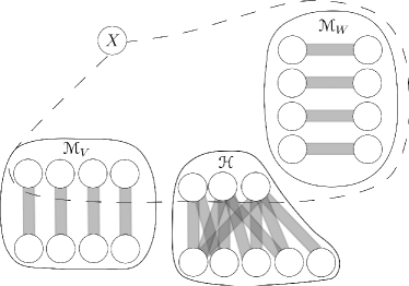
Figure 1: Structure given by Lemma 4.5

Proof.

Set $k_{0}=\frac{M_{0}}{\varepsilon}$. Apply Lemma 2.10 to $G$, with $t=(1+\delta)\frac{k}{2}$ and $\ell=|\mathscr{R}|$, to obtain a subgraph $G^{\prime}$, with a $(5\varepsilon,\eta-\varepsilon)$-regular partition into $2M_{0}$ parts whose corresponding reduced graph $\mathscr{R}^{\prime}$ contains a matching $\mathscr{M}$ and an independent set $\mathscr{I}$ with the properties stated in the lemma. By the choice of $k_{0}$ and $\varepsilon$, and by our assumption on $G$, at least $\lceil\tfrac{\delta}{2}|G^{\prime}|\rceil$ vertices of $G^{\prime}$ have degree at least $(1+\tfrac{\delta}{2})k$. So, there is a cluster $X\in V(\mathscr{R}^{\prime})$ with

$$\deg_{\mathscr{R}^{\prime}}(X)\geq(1+\tfrac{\delta}{2}){k}\tfrac{|\mathscr{R}^{\prime}|}{|G^{\prime}|}.$$ (19)

Let $\mathscr{M}_{W}$ be a maximal matching contained in $N(X)$, so that for every $CD\in\mathscr{M}_{W}$ either $CD\in\mathscr{M}$ or $C\in\mathscr{I}$ and $D\in V(\mathscr{M})$. This choice ensures that there are no edges between $\mathscr{A}:=\big{(}N_{\mathscr{R}^{\prime}}(X)\cap\mathscr{I}\big{)}\setminus V(\mathscr{M}_{W})$ and $\big{(}N_{\mathscr{R}^{\prime}}(X)\cap V(\mathscr{M})\big{)}\setminus V(\mathscr{M}_{W})$. Set $\mathscr{B}:=N_{\mathscr{R}^{\prime}}(\mathscr{A})\setminus V(\mathscr{M}_{W}).$ Let $\mathscr{M}_{V}$ consist of all edges in $\mathscr{M}-\mathscr{M}_{W}$ having one endpoint in $N(X)$.

By construction, properties $(I)-(II)$ hold, and $(III)$ holds because of (19). Finally, $(IV)$ holds because of our assumption on the minimum degree of $G$, and since any $A\in\mathscr{A}\subseteq\mathscr{I}$ sees at most one endpoint of each edge from $\mathscr{M}_{W}$. ∎

4.3 Proof of Lemma 4.1

Proof.

Given $\delta$, we choose $\varepsilon$ and $\eta$ such that $0<\varepsilon\ll\eta\ll\delta.$ Apply Lemma 2.2 with parameters $\frac{\varepsilon}{5}$ and $m_{0}=\frac{1}{\varepsilon}$ to obtain numbers $N_{0}$ and $M_{0}$. Set $k_{0}:=\max\{N_{0},\frac{2M_{0}}{\varepsilon},k^{\prime}_{0}\}$ where $k^{\prime}_{0}$ comes from Lemma 4.5, with input $\frac{\varepsilon}{5},2\eta$ and $\tfrac{\delta}{2}$. Set $\rho:=\frac{\varepsilon^{2}}{16M_{0}^{2}}$.

Given $n$, $k$ and $G$, Lemma 2.2 yields a subgraph $G^{\prime\prime}$ of $G$ with $\delta(G^{\prime\prime})\geq(1+\tfrac{\delta}{2})\frac{k}{2}$ having at least $\lceil\tfrac{\delta}{2}|G^{\prime\prime}|\rceil$ vertices of degree at least $(1+\tfrac{\delta}{2})k$, which has an $(\frac{\varepsilon}{5},2\eta)$-regular partition. Apply Lemma 4.5 to $G^{\prime\prime}$ to obtain a subgraph $G^{\prime}\subseteq G^{\prime\prime}$ having an $(\varepsilon,\eta)$-regular partition with reduced graph $\mathscr{R}^{\prime}$, which contains a cluster $X$, matchings $\mathscr{M}_{V}$ and $\mathscr{M}_{W}$, and a bipartite subgraph $\mathscr{H}=(\mathscr{A},\mathscr{B})$ satisfying properties $(I)-(IV)$.

Let $T\in\mathcal{T}(k,\rho k)$ be given, with colour classes $A,B$. Our aim is to embed $T$ into $G^{\prime}$. We may assume $|A|\geq|B|$ and choose any $r\in B$. Apply Lemma 4.3 to $(T,r)$, with $\beta=\frac{\varepsilon}{|\mathscr{R}^{\prime}|}$, to obtain a set $S\subseteq B$ with $|S|<\beta k$ and a set $\mathcal{P}$ containing all components of $T-S$.

Lemma 4.4 with $\mathcal{P}$, $|A\cap V(P)|,|B\cap V(P)|$, $M:=k-(1-11\sqrt[4]{\varepsilon})|\bigcup V(\mathscr{M}_{W})|$ and $\lambda:=\beta k$, yields a set $\mathcal{P}_{1}\subseteq\mathcal{P}$ fulfilling

1. $\sum_{P\in\mathcal{P}_{1}}a_{P}\geq\dfrac{|A\setminus S|}{|B\setminus S|}\cdot\sum_{P\in\mathcal{P}_{1}}b_{P}>\dfrac{|B|-\beta k}{|B|}\cdot\sum_{P\in\mathcal{P}_{1}}b_{P}\geq\sum_{P\in\mathcal{P}_{1}}b_{P}-\beta k$;

2. $M-\beta k\leq\sum_{P\in\mathcal{P}_{1}}|P|\leq M$;

Setting $\mathcal{P}_{2}:=\mathcal{P}\setminus\mathcal{P}_{1}$, from the first inequality in (b) we infer that

$$\textstyle\sum_{P\in\mathcal{P}_{2}}|P|\leq(1-10\sqrt[4]{\varepsilon})|\bigcup V(\mathscr{M}_{W})|.$$ (20)

Furthermore, by the second inequality in (b) and by Lemma 4.5 (III),

$$\textstyle\sum_{P^{\prime}\in\mathcal{P}_{1}}|P^{\prime}|\leq(1-10\sqrt[4]{\varepsilon})\textstyle\Big{(}\frac{|\bigcup V(\mathscr{M}_{V})|}{2}+|\bigcup\mathscr{A}|\Big{)}.$$ (21)

We will construct an embedding $\phi$ of $T$ into $G^{\prime}$ iteratively in $|S|$ steps. In each step $j$, we embed some $s_{j}\in S$ together with all subtrees ‘below’ $s_{j}$. We go through $S$ in an order that ensures our embedding remains connected throughout the process, that is, we choose $s_{1}:=r$, and for $j\geq 2$ we choose any yet unembedded $s_{j}\in S$ whose parent is already embedded. Write $U_{j}(C)$ for the set of all unused vertices in a cluster $C$ at the beginning of step $j$. Four conditions will hold throughout the embedding process:

1. If $j\geq 2$, the parent of $s_{j}$ is embedded into a vertex that is typical to $X$.

2. $|U_{j}(C)|>5\sqrt[4]{\varepsilon}|C|$ for every cluster $C$.

3. $\bigcup\mathcal{P}_{2}$ is embedded into $\bigcup V(\mathscr{M}_{W})$, $\bigcup\mathcal{P}_{1}\cap A$ is embedded into $\bigcup V(\mathscr{A}\cup(\mathscr{M}_{V}\cap N(X)))$ and $\bigcup\mathcal{P}_{1}\cap B$ is embedded into $\bigcup V(\mathscr{B}\cup(V(\mathscr{M}_{V})\setminus N(X)))$.

4. $\Big{|}|U_{j}(C)|-|U_{j}(D)|\Big{|}\leq\varepsilon|C|$ for every edge $CD\in\mathscr{M}_{W}$.

Now suppose we are at step $j\leq|S|$. Choose $s_{j}\in S$ as detailed above. Set

$$\mathscr{Y}:=\{U_{j}(C)\,:\,C\in N_{\mathscr{R}^{\prime}}(X)\cap\big{(}V(\mathscr{M}_{V})\cup V(\mathscr{M}_{W})\cup\mathscr{A}\big{)}.$$

Note that (E2) ensures that every set in $\mathscr{Y}$ is significant. Since $S$ is small, we can use Fact 2.3 (ii) to obtain a set $X^{\prime}\subset X\setminus\phi(S)$ with $|X^{\prime}|\geq(1-4\sqrt{\varepsilon})|X|$ such that

every $$v\in X^{\prime} (1-\sqrt{\varepsilon})|\mathscr{Y}| \mathscr{Y}$$ is typical to at least clusters in . (22)

If $j\geq 2$, let $w$ be the image of the parent of $s_{j}$. By (E1), $\deg(w,X)\geq\frac{\eta}{2}|X|,$ and hence $\deg(w,X^{\prime})\geq\frac{\eta}{4}|X|>\beta k>|S|.$ In particular, we can choose some vertex $v_{j}\in X^{\prime}\cap U_{j}(X)$ (adjacent to $w$, if $j\geq 2$) as $\phi(s_{j})$. Now reserve some space for the children of $s_{j}$. For each cluster $C$ such that $v_{j}$ is typical towards $U_{j}(C)$, let $C_{r}$ be any set of $2\varepsilon|C|+\rho k$ vertices in $N(v_{j})\cap U_{j}(C)$. For convenience, say $C\in V(\mathscr{R}^{\prime})$ is good if $|U_{j}(C)|\geq 7\sqrt[4]{\varepsilon}|C|$, and say $CD\in E(\mathscr{R}^{\prime})$ is good if both $C$ and $D$ are good.

It remains to embed all components of $T-S$ adjacent to $s_{j}$ that have not been embedded yet. Let $P$ be such a component. We distinguish three cases.

Case 1: $P\in\mathcal{P}_{1}$ and there are more than $\big{(}1-10\sqrt[4]{\varepsilon}\big{)}\frac{|\bigcup V(\mathscr{M}_{V})|}{2}$ unused vertices in $\bigcup V(\mathscr{M}_{V})$.

In this case there are more than $\sqrt{\varepsilon}|\mathscr{M}_{V}|$ good edges in $\mathscr{M}_{V}$. Indeed, otherwise,

$$\textstyle\big{(}1+10\sqrt[4]{\varepsilon}\big{)}\frac{|\bigcup V(\mathscr{M}_{V})|}{2} \leq\sum_{CD\in\mathscr{M}_{V},CD\text{ good}}(|U_{j}(C)\cup U_{j}(D)|)+\sum_{CD\in\mathscr{M}_{V},CD\text{ bad}}(|U_{j}(C)\cup U_{j}(D)|)$$

$$\leq\sqrt{\varepsilon}|\mathscr{M}_{V}|\cdot 2\textstyle\frac{|G^{\prime}|}{|\mathscr{R}^{\prime}|}+|\mathscr{M}_{V}|\cdot(1+7\sqrt[4]{\varepsilon})\frac{|G^{\prime}|}{|\mathscr{R}^{\prime}|},$$

a contradiction. So by (22) there is a good edge $CD\in\mathscr{M}_{V}$, with $C\in N(X)$, and $v_{j}$ typical to $U_{j}(D)$. Embed the root of $P$ into $C_{r}$ and use Lemma 2.4 to embed the remaining vertices into $(U_{j}(C)\cup U_{j}(D))\setminus(C_{r}\cup D_{r})$. In particular, all of $A\cap V(P)$ is mapped to $C$. We take care to embed parents of vertices in $S$ into vertices that are typical to $X$. So, properties (E1)-(E4) continue to hold after this step (for (E2), recall that $CD$ is good and $|P|\leq\beta k\leq\sqrt[4]{\varepsilon}|C|$).

Case 2: $P\in\mathcal{P}_{1}$ and at least $\big{(}1-10\sqrt[4]{\varepsilon}\big{)}\frac{|\bigcup V(\mathscr{M}_{V})|}{2}$ vertices of $\bigcup V(\mathscr{M}_{V})$ have been used already.

In this case, (21) ensures there are at least $10\sqrt[4]{\varepsilon}|\bigcup\mathscr{A}|$ unused vertices in $\bigcup\mathscr{A}$. So, there are more than $\sqrt{\varepsilon}|\mathscr{A}|$ good clusters in $\mathscr{A}$, as otherwise we reach a contradiction by calculating

$$\textstyle{10\sqrt[4]{\varepsilon}|\bigcup\mathscr{A}|}\leq\textstyle{\sum_{C\in\mathscr{A}}|U_{j}(C)|}\leq\textstyle\sqrt{\varepsilon}|\bigcup\mathscr{A}|+|\bigcup\mathscr{A}|7\sqrt[4]{\varepsilon}.$$

By (22), $v_{j}$ is typical towards $U_{j}(C)$ for some good $C\in\mathscr{A}$. Moreover, there is a good cluster $D\in N_{\mathscr{R}^{\prime}}(C)\cap\mathscr{B}$, as otherwise we must have already used more than

$$\textstyle(1-7\sqrt[4]{\varepsilon})\deg_{\mathscr{R}^{\prime}}(C,\mathscr{B})\cdot\frac{|G^{\prime}|}{|\mathscr{R}^{\prime}|} \geq\textstyle(1-7\sqrt[4]{\varepsilon})\cdot\tfrac{1}{2}\big{(}(1+\tfrac{\delta}{4})k-|\bigcup V(\mathscr{M_{W}})|\big{)}$$

$$\geq\textstyle\tfrac{1}{2}\big{(}k-(1-11\sqrt[4]{\varepsilon})|\bigcup V(\mathscr{M_{W}})|\big{)}$$

$$\textstyle>\frac{1}{2}\cdot\sum_{P^{\prime}\in\mathcal{P}_{1}}|P^{\prime}|$$

vertices of $\bigcup\mathscr{B}$ (where the first inequality comes from Lemma 4.5 (IV), and the last one from the second inequality in (b)). But this is impossible since by (E3) and by (a), we know that $\bigcup\mathscr{A}$ hosts at least as many vertices from $V(\bigcup\mathcal{P}_{1})$ as $\bigcup\mathscr{B}$ does, up to an error term of $\beta k$.

Embed the root of $P$ into $C_{r}$ and use Lemma 2.4 to embed the rest of $P$ into $(U_{j}(C)\cup U_{j}(D))\setminus(C_{r}\cup D_{r})$. Parents of vertices in $S$ are embedded into vertices that are typical to $X$.

Case 3: $P\in\mathcal{P}_{2}$.

Using (20) and (E4) we see as above there is a good edge $CD\in\mathscr{M}_{W}$, with $v_{j}$ typical to both $U_{j}(C)$ and $U_{j}(D)$. Embed $P$ into $U_{j}(C)\cup U_{j}(D)$ avoiding $C_{r}\cup D_{r}$, except for the root $r_{P}$ of $P$. Note that we can choose into which of $C_{r}$ or $D_{r}$ we embed $r_{P}$, and we choose wisely so that after the embedding of $P$, (E4) still holds. As always, we embed parents of vertices in $S$ into vertices that are typical to $X$. This finishes the embedding for Case 3, and thus the proof of Lemma 4.1. ∎

Appendix A Concentration lemmas

In this appendix we prove two results on the concentration of a given function around its mean value. Given $N\in\mathbb{N}$ and a function $f:[N]\to\mathbb{R}$, we write

$$\|f\|_{\infty}=\max_{n\in[N]}|f(n)|$$

for the infinity norm of $f$. If $\mu$ is a probability measure on $[N]$ then, as usual,

$${\mathbb{E}}_{\mu}(f)=\sum_{n\in[N]}f(n)\mu(n)$$

denotes the expectation of $f$ under $\mu$, and if $\mu$ is the uniform probability we write

$$\mathbb{E}_{n\in[N]}f(n)=\frac{1}{N}\sum_{n\in[N]}f(n).$$

Lemma A.1.

Let $N\in\mathbb{N}$, $t\in\mathbb{R}$ and $\varepsilon\in(0,1)$. Let $\mu$ be a probability measure on $[N]$ and let $f:[N]\to\mathbb{R}_{+}$ satisfying $\sqrt{\varepsilon}\|f\|_{\infty}<t\leq{\mathbb{E}}_{\mu}(f).$ Then at least one of the following holds

1. $\mu(\{n:f(n)>(1+\sqrt{\varepsilon})t\})\geq\varepsilon$, or

2. $\mu(\{n:f(n)>(1-\sqrt[4]{\varepsilon})t\})\geq 1-\sqrt[4]{\varepsilon}$.

Proof.

Let $A$ be the set of all $n\in[N]$ with $f(n)>(1+\sqrt{\varepsilon})t$ and set $B:=[N]\setminus A$. Suppose that (i) does not hold. Then $\mu(A)\leq\varepsilon$, and therefore,

$$\sum_{n\in B}\mu(n)f(n)={\mathbb{E}}_{\mu}(f)-\sum_{n\in A}\mu(n)f(n)\geq t-\mu(A)\|f\|_{\infty}\geq(1-\sqrt{\varepsilon})t.$$ (23)

Let $B_{1}$ be the set of all $n\in B$ such that $f(n)<(1+\sqrt{\varepsilon}-2\sqrt[4]{\varepsilon})t$, and set $B_{2}:=B\setminus B_{1}$. From (23) and the definition of $B$ we deduce that

$$(1-\sqrt{\varepsilon})t\leq(1+\sqrt{\varepsilon})t\cdot\mu(B)-2\sqrt[4]{\varepsilon}t\cdot\mu(B_{1})\leq(1+\sqrt{\varepsilon})t-2\sqrt[4]{\varepsilon}t\cdot\mu(B_{1}),$$

and hence, $\mu(B_{1})\leq\sqrt[4]{\varepsilon}$. Therefore, $\mu(A\cup B_{2})\geq 1-\mu(B_{1})\geq 1-\sqrt[4]{\varepsilon},$ which implies (ii).∎

As a corollary of Lemma A.1 we get the following useful result.

Lemma A.2.

Let $N\in\mathbb{N}$, and let $\varepsilon\in(0,\frac{1}{2})$. Let $f:[N]\to\mathbb{R}_{+}$ be a function and let $t>0$ such that $t\leq{\mathbb{E}}_{n\in[N]}f(n)$ and $\|f\|_{\infty}\leq(1+\varepsilon)t$. Then $f(n)\geq(1-\sqrt{\varepsilon})t$ for every $n$ in a set of size at least $(1-\sqrt{\varepsilon})N$.

References

- [1] Ajtai, M., Komlós, J., and Szemerédi, E. On a conjecture of Loebl. In Graph theory, combinatorics, and algorithms, Vol. 1, 2 (Kalamazoo, MI, 1992), Wiley-Intersci. Publ. Wiley, New York, 1995, pp. 1135–1146.
- [2] Besomi, G., Pavez-Signé, M., and Stein, M. Degree conditions for embedding trees. SIAM J. Discrete Math. 33, 3 (2019), 1521–1555.
- [3] Brandt, S., and Dobson, E. The Erdős–Sós conjecture for graphs of girth . Discrete Math. 150 (1996), 411–414.
- [4] Erdős, P. Extremal problems in graph theory. In Theory of graphs and its applications, Proc. Sympos. Smolenice (1964), pp. 29–36.
- [5] Erdős, P., and Gallai, T. On maximal paths and circuits of graphs. Acta Math. Acad. Sci. Hungar. 10, 3 (1959), 337–356.
- [6] Erdős, P., and Graham, R. L. On partition theorems for finite graphs. In Infinite and finite sets (Colloq. Keszthely, 1973; dedicated to P. Erdős on his 60th birthday), vol. 10. Colloq. Math. Soc. János Bolyai, 1975, pp. 515–527.
- [7] Goerlich, A., and Zak, A. On Erdős-Sós Conjecture for Trees of Large Size. Electron. J. Combin. 23, 1 (2016), P1–52.
- [8] Havet, F., Reed, B., Stein, M., and Wood, D. R. A variant of the Erdős–Sós conjecture. J. Graph Theory 94, 1 (2020), 131–158.
- [9] Hladký, J., Komlós, J., Piguet, D., Simonovits, M., Stein, M., and Szemerédi, E. The Approximate Loebl–Komlós–Sós Conjecture IV: Embedding Techniques and the Proof of the Main Result. SIAM J. Discrete Math. 31, 2 (2017), 1072–1148.
- [10] Komlós, J., Shokoufandeh, A., Simonovits, M., and Szemerédi, E. The regularity lemma and its applications in graph theory. In Theoretical Aspects of Computer Science, Advanced Lectures (2000), pp. 84–112.
- [11] Krivelevich, M. Embedding spanning trees in random graphs. SIAM J. Discrete Math. 24, 4 (2010), 1495–1500.
- [12] Montgomery, R. Spanning trees in random graphs. Adv. Math. 356 (2019), 106793.
- [13] Reed, B., and Stein, M. Spanning trees in graphs of high minimum degree with a universal vertex I: An approximate asymptotic result. Preprint 2019, arXiv 1905.09801.
- [14] Rozhoň, V. A local approach to the Erdős–Sós conjecture. SIAM J. Discrete Math. 33, 2 (2019), 643–664.
- [15] Saclé, J.-F., and Woźniak, M. A note on the Erdős–Sós conjecture for graphs without . J. Combin. Theory (Series B) 70, 2 (1997), 229–234.
- [16] Szemerédi, E. Regular partitions of graphs. In Problèmes combinatoires et théorie des graphes (Colloq. Internat. CNRS, Univ. Orsay, Orsay, 1976), vol. 260 of Colloq. Internat. CNRS. CNRS, Paris, 1978, pp. 399–401.