A Stochastic Composite Gradient Method with Incremental Variance Reduction

Abstract

We consider the problem of minimizing the composition of a smooth (nonconvex) function and a smooth vector mapping, where the inner mapping is in the form of an expectation over some random variable or a finite sum. We propose a stochastic composite gradient method that employs an incremental variance-reduced estimator for both the inner vector mapping and its Jacobian. We show that this method achieves the same orders of complexity as the best known first-order methods for minimizing expected-value and finite-sum nonconvex functions, despite the additional outer composition which renders the composite gradient estimator biased. This finding enables a much broader range of applications in machine learning to benefit from the low complexity of incremental variance-reduction methods.

1 Introduction

We consider stochastic composite optimization problems of the form

$$\mathop{\textrm{minimize}}_{x\in\mathbf{R}^{d}}\quad f\bigl{(}\mathbf{E}_{\xi}[g_{\xi}(x)]\bigr{)}+r(x)\,,$$ (1)

where $f:\mathbf{R}^{p}\to\mathbf{R}$ is a smooth and possibly nonconvex function, $\xi$ is a random variable, each $g_{\xi}:\mathbf{R}^{d}\to\mathbf{R}^{p}$ is a smooth vector mapping, and $r$ is convex and lower-semicontinuous. A special case we will consider separately is when $\xi$ is a discrete random variable with uniform distribution over $\{1,2,\ldots,n\}$. In this case the problem is equivalent to a deterministic optimization problem

$$\mathop{\textrm{minimize}}_{x\in\mathbf{R}^{d}}\quad f\biggl{(}\frac{1}{n}\sum_{i=1}^{n}g_{i}(x)\biggr{)}+r(x)\,.$$ (2)

The formulations in (1) and (2) cover a broader range of applications than classical stochastic optimization and empirical risk minimization (ERM) problems where each $g_{\xi}$ is a scalar function ($p=1$) and $f$ is the scalar identity map. A well-known example is policy evaluation in reinforcement learning (RL) [e.g., 29]. With linear value function approximation, it can be formulated as

$$\mathop{\textrm{minimize}}_{x\in\mathbf{R}^{d}}\quad\bigl{\|}\mathbf{E}[A]x-\mathbf{E}[b]\bigr{\|}^{2},$$

where $A$ and $b$ are random matrix and vector generated by a Markov decision process (MDP) [e.g., 6]. Here we have $f(\cdot)=\|\cdot\|^{2}$, $\xi=(A,b)$ and $g_{\xi}(x)=Ax-b$.

Another interesting application is risk-averse optimization [e.g., 27, 28], which has many applications in RL and financial mathematics. We consider a general formulation of mean-variance trade-off:

$$\mathop{\textrm{maximize}}_{x\in\mathbf{R}^{d}}~{}~{}\left\{\,\mathbf{E}\bigl{[}h_{\xi}(x)\bigr{]}-\lambda\mathbf{Var}\bigl{(}h_{\xi}(x)\bigr{)}~{}\equiv~{}\mathbf{E}\bigl{[}h_{\xi}(x)\bigr{]}-\lambda\Bigl{(}\mathbf{E}\bigl{[}h_{\xi}^{2}(x)\bigr{]}-\mathbf{E}\bigl{[}h_{\xi}(x)\bigr{]}^{2}\Bigr{)}\right\},$$ (3)

where each $h_{\xi}(x):\mathbf{R}^{d}\to\mathbf{R}$ is a reward function (such as total portfolio return). The goal of problem (3) is to maximize the average reward with a penalty on the variance which captures the potential risk. It can be cast in the form of (1) by using the mappings

$$g_{\xi}(x):\mathbf{R}^{d}\to\mathbf{R}^{2}=\bigl{[}h_{\xi}(x)~{}~{}h^{2}_{\xi}(x)\bigr{]}^{T},\qquad f(y,z):\mathbf{R}^{2}\to\mathbf{R}=-y+\lambda y^{2}-\lambda z\,.$$ (4)

Here, the intermediate dimension is very low, i.e., $p=2$. This leads to very little overhead in computation compared with stochastic optimization without composition.

Besides these applications, the composition structure in (1) and (2) are of independent interest for research on stochastic and randomized algorithms. For the ease of notation, we define

$$g(x):=\mathbf{E}_{\xi}[g_{\xi}(x)],\qquad F(x):=f(g(x)),\qquad\Phi(x):=F(x)+r(x).$$ (5)

In addition, let $f^{\prime}$ and $F^{\prime}$ denote the gradients of $f$ and $F$ respectively, and $g^{\prime}_{\xi}(x)\in\mathbf{R}^{p\times d}$ denote the Jacobian matrix of $g_{\xi}$ at $x$. Then we have

$$F^{\prime}(x)=\nabla\Bigl{(}f\bigl{(}\mathbf{E}_{\xi}[g_{\xi}(x)]\bigr{)}\Bigr{)}=\Bigl{(}\mathbf{E}_{\xi}[g^{\prime}_{\xi}(x)]\Bigr{)}^{T}f^{\prime}\bigl{(}\mathbf{E}_{\xi}[g_{\xi}(x)]\bigr{)}\,.$$

In practice, computing $F^{\prime}(x)$ exactly can be very costly if not impossible. A common strategy is to use stochastic approximation: we randomly sample a subset $\mathcal{S}$ of $\xi$ from its distribution and let

$$\tilde{g}(x)=\frac{1}{|\mathcal{S}|}\sum_{\xi\in\mathcal{S}}g_{\xi}(x),\qquad\tilde{g^{\prime}}(x)=\frac{1}{|\mathcal{S}|}\sum_{\xi\in\mathcal{S}}g^{\prime}_{\xi}(x).$$ (6)

However, $\left(\tilde{g^{\prime}}(x)\right)^{T}\!f(\tilde{g}(x))$ is always a biased estimate of $F^{\prime}(x)$ unless one can replace $\tilde{g}(x)$ with the full expectation $\mathbf{E}_{\xi}[g_{\xi}(x)]$. This is in great contrast to the classical stochastic optimization problem

$$\mathop{\textrm{minimize}}_{x\in\mathbf{R}^{d}}\quad\mathbf{E}_{\xi}\bigl{[}g_{\xi}(x)\bigr{]}+r(x)\,,$$ (7)

where $\tilde{g^{\prime}}(x)$ in (6) is always an unbiased gradient estimator for the smooth part $g(x)=\mathbf{E}_{\xi}\bigl{[}g_{\xi}(x)\bigr{]}$. Using biased gradient estimators can cause various difficulties for constructing and analyzing randomized algorithms, but is often inevitable in dealing with more complex objective functions other than the empirical risk [see, e.g., 5, 11, 10, 18]. As a simplest model, the analysis of randomized algorithms for (1) may provide insights for solving more challenging problems.

In this paper, we develop an efficient stochastic composite gradient method called CIVR (Composite Incremental Variance Reduction), for solving problems of the forms (1) and (2). We measure efficiency by the sample complexity of the individual functions $g_{\xi}$ and their Jacobian $g^{\prime}_{\xi}$, i.e., the total number of times they need to be evaluated at some point, in order to find an $\epsilon$-approximate solution. For nonconvex functions, an $\epsilon$-approximate solution is some random output of the algorithm $\bar{x}\in\mathbf{R}^{d}$ that satisfies $\mathbf{E}[\|\mathcal{G}(\bar{x})\|^{2}]\leq\epsilon$, where $\mathcal{G}(\bar{x})$ is the proximal gradient mapping of the objective function $\Phi$ at $\bar{x}$ (see details in Section 2). If $r\equiv 0$, then $\mathcal{G}(\bar{x})=F^{\prime}(\bar{x})$ and the criteria for $\epsilon$-approximation becomes $\mathbf{E}[\|F^{\prime}(\bar{x})\|^{2}]\leq\epsilon$. If the objective $\Phi$ is convex, we require $\mathbf{E}[\Phi(\bar{x})-\Phi^{\star}]\leq\epsilon$ where $\Phi^{\star}=\inf_{x}\Phi(x)$. For smooth and convex functions, these two notions are compatible, meaning that the dependence of the sample complexity on $\epsilon$ in terms of both notions are of the same order.

Table 1: Sample complexities of CIVR (Composite Incremental Variance Reduction)

	Assumptions (common: $f$ and $g_{\xi}$ Lipschitz and smooth, thus $F$ smooth)
Problem	$F$ nonconvex	$F$ $\nu$-gradient dominant	$F$ convex, $r$ convex
	$r$ convex	$r\equiv 0$	$\Phi$ $\mu$-optimally strongly convex
(1)	${\mathcal{O}}\bigl{(}\epsilon^{-3/2}\bigr{)}$	${\mathcal{O}}\left(\bigl{(}\nu\epsilon^{-1}\bigr{)}\log\epsilon^{-1}\right)$	${\mathcal{O}}\left(\bigl{(}\mu^{-1}\epsilon^{-1}\bigr{)}\log\epsilon^{-1}\right)$
(2)	${\mathcal{O}}\bigl{(}\min\{\epsilon^{-3/2},\,n^{1/2}\epsilon^{-1}\}\bigr{)}$	${\mathcal{O}}\left(\bigl{(}n+\nu n^{1/2}\bigr{)}\log\epsilon^{-1}\right)$	${\mathcal{O}}\left(\bigl{(}n+\mu^{-1}n^{1/2}\bigr{)}\log\epsilon^{-1}\right)$

Table 1 summarizes the sample complexities of the CIVR method under different assumptions obtained in this paper. We can define a condition number $\kappa={\mathcal{O}}(\nu)$ for $\nu$-gradient dominant functions and $\kappa={\mathcal{O}}(1/\mu)$ for $\mu$-optimally strongly convex functions, then the complexities become ${\mathcal{O}}\bigl{(}\bigl{(}\kappa\epsilon^{-1}\bigr{)}\log\epsilon^{-1}\bigr{)}$ and ${\mathcal{O}}\bigl{(}\bigl{(}n+\kappa n^{1/2}\bigr{)}\log\epsilon^{-1}\bigr{)}$ for (1) and (2) respectively. In order to better position our contributions, we next discuss related work and then putting these results into context.

1.1 Related Work

We first discuss the nonconvex stochastic optimization problem (7), which is a special cases of (1). When $r\!\equiv\!0$ and $g(x)\!=\!\mathbf{E}_{\xi}[g_{\xi}(x)]$ is smooth, Ghadimi and Lan [9] developed a randomized stochastic gradient method with iteration complexity ${\mathcal{O}}(\epsilon^{-2})$. Allen-Zhu [2] obtained ${\mathcal{O}}\bigl{(}\epsilon^{-1.625}\bigr{)}$ with additional second-order guarantee. There are also many recent works on solving its finite-sum version

$$\mathop{\textrm{minimize}}_{x\in\mathbf{R}^{d}}\quad\frac{1}{n}\sum_{i=1}^{n}g_{i}(x)+r(x),$$ (8)

which is a special case of (2). By extending the variance reduction techniques SVRG [13, 33] and SAGA [7] to nonconvex optimization, Allen-Zhu and Hazan [3] and Reddi et al. [23, 24, 25] developed randomized algorithms with sample complexity ${\mathcal{O}}(n+n^{2/3}\epsilon^{-1})$. Under additional assumptions of gradient dominance or strong convexity, they obtained sample complexity ${\mathcal{O}}((n+\kappa n^{2/3})\log\epsilon^{-1})$, where $\kappa$ is a suitable condition number. Allen-Zhu [1] and Lei et al. [15] obtained ${\mathcal{O}}\bigl{(}\min\{\epsilon^{-5/3},\,n^{2/3}\epsilon^{-1}\}\bigr{)}$.

Based on a new variance reduction technique called SARAH [20], Nguyen et al. [21] and Pham et al. [22] developed nonconvex extensions to obtain sample complexities ${\mathcal{O}}\bigl{(}\epsilon^{-3/2}\bigr{)}$ and ${\mathcal{O}}\bigl{(}n+n^{1/2}\epsilon^{-1}\bigr{)}$ for solving the expectation and finite-sum cases respectively. Fang et al. [8] introduced another variance reduction technique called Spider, which can be viewed as a more general variant of SARAH. They obtained sample complexities ${\mathcal{O}}\bigl{(}\epsilon^{-3/2}\bigr{)}$ and ${\mathcal{O}}\bigl{(}\min\{\epsilon^{-3/2},\,n^{1/2}\epsilon^{-1}\}\bigr{)}$ for the two cases respectively, but require small step sizes that are proportional to $\epsilon$. Wang et al. [32] extended Spider to obtain the same complexities with constant step sizes and ${\mathcal{O}}\bigl{(}(n+\kappa^{2})\log\epsilon^{-1}\bigr{)}$ under the gradient-dominant condition. In addition, Zhou et al. [35] obtained similar results using a nested SVRG approach.

In addition to the above works on solving special cases of (1) and (2), there are also considerable recent works on a more general, two-layer stochastic composite optimization problem

$$\mathop{\textrm{minimize}}_{x\in\mathbf{R}^{d}}\quad\mathbf{E}_{\nu}\bigl{[}f_{\nu}\left(\mathbf{E}_{\xi}[g_{\xi}(x)]\right)\bigr{]}+r(x)\,,$$ (9)

where $f_{\nu}$ is parametrized by another random variables $\nu$, which is independent of $\xi$. When $r\equiv 0$, Wang et al. [30] derived algorithms to find an $\epsilon$-approximate solution with sample complexities ${\mathcal{O}}(\epsilon^{-4})$, ${\mathcal{O}}(\epsilon^{-3.5})$ and ${\mathcal{O}}(\epsilon^{-1.25})$ for the smooth nonconvex case, smooth convex case and smooth strongly convex case respectively. For nontrivial convex $r$, Wang et al. [31] obtained improved sample complexity of ${\mathcal{O}}(\epsilon^{-2.25})$, ${\mathcal{O}}(\epsilon^{-2})$ and ${\mathcal{O}}(\epsilon^{-1})$ for the three cases mentioned above respectively.

As a special case of (9), the following finite-sum problem also received significant attention:

$$\mathop{\textrm{minimize}}_{x\in\mathbf{R}^{d}}\quad\frac{1}{m}\sum_{j=1}^{m}f_{j}\biggl{(}\frac{1}{n}\sum_{i=1}^{n}g_{i}(x)\biggr{)}+r(x)\,.$$ (10)

When $r\equiv 0$ and the overall objective function is strongly convex, Lian et al. [17] derived two algorithms based on the SVRG scheme to attain sample complexities ${\mathcal{O}}((m+n+\kappa^{3})\log\epsilon^{-1}))$ and ${\mathcal{O}}((m+n+\kappa^{4})\log\epsilon^{-1}))$ respectively, where $\kappa$ is some suitably defined condition number. Huo et al. [12] also used the SVRG scheme to obtain an ${\mathcal{O}}(m+n+(m+n)^{2/3}\epsilon^{-1})$ complexity for the smooth nonconvex case and ${\mathcal{O}}((m+n+\kappa^{3})\log\epsilon^{-1}))$ for strongly convex problems with nonsmooth $r$. More recently, Zhang and Xiao [34] proposed a composite randomized incremental gradient method based on the SAGA estimator [7], which matches the best known ${\mathcal{O}}(m+n+(m+n)^{2/3}\epsilon^{-1})$ complexity when $F$ is smooth and nonconvex, and obtained an improved complexity ${\mathcal{O}}\bigl{(}(m+n+\kappa(m+n)^{2/3})\log\epsilon^{-1}\bigr{)}$ under either gradient dominant or strongly convex assumptions. When applied to the special cases (1) and (2) we focus on in this paper ($m=1$), these results are strictly worse than ours in Table 1.

1.2 Contributions and Outline

We develop the CIVR method by extending the variance reduction technique of SARAH [20, 21, 22] and Spider [8, 32] to solve the composite optimization problems (1) and (2). The complexities of CIVR in Table 1 match the best results for solving the non-composite problems (7) and (8), despite the additional outer composition and the composite-gradient estimator always being biased. In addition:

• It is shown in [8] that the ${\mathcal{O}}\bigl{(}\min\{\epsilon^{-3/2},\,n^{1/2}\epsilon^{-1}\}\bigr{)}$ complexity is nearly optimal for the non-composite finite-sum optimization problem (8). Therefore, we do not expect algorithms with better complexity for solving the more general composite finite-sum problem (2).

• Under the assumptions of gradient dominance or strong convexity, the ${\mathcal{O}}\bigl{(}\bigl{(}n\!+\!\kappa n^{1/2}\bigr{)}\log\epsilon^{-1}\bigr{)}$ complexity only appeared for the special case (8) in the recent work [16].

Our results indicate that the additional smooth composition in (1) and (2) does not incur higher complexity compared with (7) and (8), despite the difficulty of dealing with biased estimators. We believe these results can also be extended to the two-layer problems (9) and (10), by replacing $n$ with $m+n$ in Table 1. But the extensions require quite different techniques and we will address them in a separate paper.

The rest of this paper is organized as follows. In Section 2, we introduce the CIVR method. In Section 3, we present convergence results of CIVR for solving the composite optimization problems (1) and (2) and the required parameter settings. Better complexities of CIVR under the gradient-dominant and optimally strongly convex conditions are given in Section 4. In Section 5, we present numerical experiments for solving a risk-averse portfolio optimization problem (3) on real-world datasets.

2 The composite incremental variance reduction (CIVR) method

input: initial point $x^{1}_{0}$, step size $\eta>0$, number of epochs $T\geq 1$, and a set of triples $\{\tau_{t},B_{t},S_{t}\}$ for $t=1,\ldots,T$, where $\tau_{t}$ is the epoch length and $B_{t}$ and $S_{t}$ are sample sizes in epoch $t$.

for $t=1,...,T$ do

       Sample a set $\mathcal{B}_{t}$ with size $B_{t}$ from the distribution of $\xi$, and construct the estimates

      

$$y_{0}^{t}=\frac{1}{B_{t}}\sum_{\xi\in\mathcal{B}_{t}}g_{\xi}(x_{0}^{t}),\qquad z_{0}^{t}=\frac{1}{B_{t}}\sum_{\xi\in\mathcal{B}_{t}}g_{\xi}^{\prime}(x_{0}^{t}),\qquad$$ (11)

Compute $\tilde{\nabla}F(x_{0}^{t})=(z_{0}^{t})^{T}f^{\prime}(y_{0}^{t})$ and update: $x_{1}^{t}=\mathbf{prox}_{r}^{\eta}\bigl{(}x_{0}^{t}-\eta\tilde{\nabla}F(x_{0}^{t})\bigr{)}$.

       for $i=1,...,\tau_{t}-1$ do

             Sample a set $\mathcal{S}_{i}^{t}$ with size $S_{t}$ from the distribution of $\xi$, and construct the estimates

            [-2ex]

$$y_{i}^{t} = y_{i-1}^{t}+\frac{1}{S_{t}}\sum_{\xi\in\mathcal{S}_{i}^{t}}\left(g_{\xi}(x_{i}^{t})-g_{\xi}(x_{i-1}^{t})\right),$$ (12)

$$z_{i}^{t} = z_{i-1}^{t}\,+\,\frac{1}{S_{t}}\sum_{\xi\in\mathcal{S}_{i}^{t}}\bigl{(}g^{\prime}_{\xi}(x_{i}^{t})-g^{\prime}_{\xi}(x_{i-1}^{t})\bigr{)}.$$ (13)

Compute $\tilde{\nabla}F(x_{i}^{t})=(z_{i}^{t})^{T}f^{\prime}(y_{i}^{t})$ and update: $x_{i+1}^{t}=\mathbf{prox}_{r}^{\eta}\bigl{(}x_{i}^{t}-\eta\tilde{\nabla}F(x_{i}^{t})\bigr{)}$.

            

       end for

      Set $x_{0}^{t+1}=x_{\tau_{t}}^{t}$.

      

end for

output: $\bar{x}$ randomly chosen from $\bigl{\{}x_{i}^{t}\bigr{\}}_{i=0,...,\tau_{t}-1}^{t=1,...,T}$.

Algorithm 1 Composite Incremental Variance Reduction (CIVR)

With the notations in (5), we can write the composite stochastic optimization problem (1) as

$$\mathop{\textrm{minimize}}_{x\in\mathbf{R}^{d}}\quad\bigl{\{}\Phi(x)=F(x)+r(x)\bigr{\}}\,,$$ (14)

where $F$ is smooth and $r$ is convex. The proximal operator of $r$ with parameter $\eta$ is defined as

$$\mathbf{prox}^{\eta}_{r}(x):=\mathop{\rm argmin}_{y}\,\Bigl{\{}r(y)+\frac{1}{2\eta}\|y-x\|^{2}\Bigr{\}}.$$ (15)

We assume that $r$ is relatively simple, meaning that its proximal operator has a closed-form solution or can be computed efficiently. The proximal gradient method [e.g., 19, 4] for solving problem (14) is

$$x^{t+1}=\mathbf{prox}_{r}^{\eta}\bigl{(}x^{t}-\eta F^{\prime}(x^{t})\bigr{)}\,,$$ (16)

where $\eta$ is the step size. The proximal gradient mapping of $\Phi$ is defined as

$$\mathcal{G}_{\eta}(x)\triangleq\frac{1}{\eta}\Bigl{(}x-\mathbf{prox}^{\eta}_{r}\bigl{(}x-\eta F^{\prime}(x)\bigr{)}\Bigr{)}.$$ (17)

As a result, the proximal gradient method (16) can be written as $x^{t+1}=x^{t}-\eta\,\mathcal{G}(x^{t})$. Notice that when $r\equiv 0$, $\mathbf{prox}_{r}^{\eta}(\cdot)$ becomes the identity mapping and we have $\mathcal{G}_{\eta}(x)\equiv F^{\prime}(x)$ for any $\eta>0$.

Suppose $\bar{x}$ is generated by a randomized algorithm. We call $\bar{x}$ an $\epsilon$-stationary point in expectation if

$$\mathbf{E}\bigl{[}\|\mathcal{G}_{\eta}(\bar{x})\|^{2}\bigr{]}\leq\epsilon.$$ (18)

(We assume that $\eta$ is a constant that does not depend on $\epsilon$.) As we mentioned in the introduction, we measure the efficiency of an algorithm by its sample complexity of $g_{\xi}$ and their Jacobian $g^{\prime}_{\xi}$, i.e., the total number of times they need to be evaluated, in order to find a point $\bar{x}$ that satisfies (18). Our goal is to develop a randomized algorithm that has low sample complexity.

We present in Algorithm 1 the Composite Incremental Variance Reduction (CIVR) method. This methods employs a two time-scale variance-reduced estimator for both the inner function value of $g(\cdot)=\mathbf{E}_{\xi}[g_{\xi}(\cdot)]$ and its Jacobian $g^{\prime}(\cdot)$. At the beginning of each outer iteration $t$ (each called an epoch), we construct a relatively accurate estimate $y_{0}^{t}$ for $g(x_{0}^{t})$ and $z_{0}^{t}$ for $g^{\prime}(x_{0}^{t})$ respectively, using a relatively large sample size $B_{t}$. During each inner iteration $i$ of the $t$th epoch, we construct an estimate $y_{i}^{t}$ for $g(x_{i}^{t})$ and $z_{i}^{t}$ for $g^{\prime}(x_{i}^{t})$ respectively, using a smaller sample size $S_{t}$ and incremental corrections from the previous iterations. Note that the epoch length $\tau_{t}$ and the sample sizes $B_{t}$ and $S_{t}$ are all adjustable for each epoch $t$. Therefore, besides setting a constant set of parameters, we can also adjust them gradually in order to obtain better theoretical properties and practical performance.

This variance-reduction technique was first proposed as part of SARAH [20] where it is called recursive variance reduction. It was also proposed in [8] in the form of a Stochastic Path-Integrated Differential EstimatoR (Spider). Here we simply call it incremental variance reduction. A distinct feature of this incremental estimator is that the inner-loop estimates $y_{i}^{t}$ and $z_{i}^{t}$ are biased, i.e.,

$$\begin{cases}~{}\mathbf{E}[y_{i}^{t}|x_{i}^{t}]=g(x_{i}^{t})-g(x_{i-1}^{t})+y_{i-1}^{t}\neq g(x_{i}^{t})\,,\\ ~{}\mathbf{E}[z_{i}^{t}|x_{i}^{t}]=g^{\prime}(x_{i}^{t})-g^{\prime}(x_{i-1}^{t})+z_{i-1}^{t}\neq g^{\prime}(x_{i}^{t})\,.\end{cases}$$ (19)

This is in contrast to two other popular variance-reduction techniques, SVRG [13] and SAGA [7], whose gradient estimators are always unbiased. Note that unbiased estimators for $g(x_{i}^{t})$ and $g^{\prime}(x_{i}^{t})$ are not essential here, because the composite estimator $\tilde{\nabla}F(x_{i}^{t})=(z_{i}^{t})^{T}f^{\prime}(y_{i}^{t})$ is always biased.

3 Convergence Analysis

In this section, we present theoretical results on the convergence properties of CIVR (Algorithm 1) when the composite function $F$ is smooth. More specifically, we make the following assumptions.

Assumption 1.

The following conditions hold concerning problems (1) and (2):

• $f:\mathbf{R}^{p}\rightarrow\mathbf{R}$ is a $C^{1}$ smooth and $\ell_{f}$-Lipschitz function and its gradient $f^{\prime}$ is $L_{f}$-Lipschitz.

• Each $g_{\xi}:\mathbf{R}^{d}\rightarrow\mathbf{R}^{p}$ is a $C^{1}$ smooth and $\ell_{g}$-Lipschitz vector mapping and its Jacobian $g_{\xi}^{\prime}$ is $L_{g}$-Lipschtiz. Consequently, $g$ in (5) is $\ell_{g}$-Lipschitz and its Jacobian $g^{\prime}$ is $L_{g}$-Lipschitz.

• $r:\mathbf{R}^{d}\rightarrow\mathbf{R}\cup\{\infty\}$ is a convex and lower-semicontinuous function.

• The overall objective function $\Phi$ is bounded below, i.e., $\Phi^{*}=\inf_{x}\Phi(x)>-\infty$.

Assumption 2.

For problem (1), we further assume that there exist constants $\sigma_{g}$ and $\sigma_{g^{\prime}}$ such that

$$\mathbf{E}_{\xi}[\|g_{\xi}(x)-g(x)\|^{2}]\leq\sigma_{g}^{2}\,,\qquad\mathbf{E}_{\xi}[\|g^{\prime}_{\xi}(x)-g^{\prime}(x)\|^{2}]\leq\sigma_{g^{\prime}}^{2}\,.$$ (20)

As a result of Assumption 1, $F(x)=f\bigl{(}g(x)\bigr{)}$ is smooth and $F^{\prime}$ is $L_{F}$-Lipschitz continuous with

$$L_{F}=\ell_{g}^{2}L_{f}+\ell_{f}L_{g}$$

(see proof in the supplementary materials). For convenience, we also define two constants

$$G_{0}:=2\bigl{(}\ell_{g}^{4}L_{f}^{2}+\ell_{f}^{2}L_{g}^{2}\bigr{)}\,,\qquad\mbox{and}\qquad\sigma_{0}^{2}:=2\bigl{(}\ell_{g}^{2}L_{f}^{2}\sigma_{g}^{2}+\ell_{f}^{2}\sigma_{g^{\prime}}^{2}\bigr{)}\,.$$ (21)

It is important to notice that $G_{0}={\mathcal{O}}(L_{F}^{2})$, since we will use step size $\eta=\Theta(1/\sqrt{G_{0}})=\Theta(1/L_{F})$.

In the next two subsections, we present complexity analysis of CIVR for solving problem (1) and (2) respectively. Due to the space limitation, all proofs are provided in the supplementary materials.

3.1 The composite expectation case

The following results for solving problem (1) are presented with notations defined in (5), (17) and (21).

Theorem 1.

Suppose Assumptions 1 and 2 hold. Given any $\epsilon>0$, we set $T=\lceil 1/\sqrt{\epsilon}\rceil$ and

$$\tau_{t}=\tau=\lceil 1/\sqrt{\epsilon}\rceil,\quad B_{t}=B=\lceil\sigma_{0}^{2}/\epsilon\rceil,\quad S_{t}=S=\lceil 1/\sqrt{\epsilon}\rceil,\quad\mbox{for}\quad t=1,\ldots,T.$$

Then as long as $\eta\leq\frac{4}{L_{F}+\sqrt{L_{F}^{2}+12G_{0}}}$, the output $\bar{x}$ of Algorithm 1 satisfies

$$\mathbf{E}\bigl{[}\|\mathcal{G}_{\eta}(\bar{x})\|^{2}\bigr{]}\leq\Bigl{(}8\bigl{(}\Phi(x_{0}^{1})-\Phi^{*}\bigr{)}\eta^{-1}+6\Bigr{)}\cdot\epsilon={\mathcal{O}}(\epsilon).$$ (22)

As a result, the sample complexity of obtaining an $\epsilon$-approximate solution is $TB+2T\tau S={\mathcal{O}}\bigl{(}\epsilon^{-3/2}\bigr{)}$.

Note that in the above scheme, the epoch lengths $\tau_{t}$ and all the batch sizes $B_{t}$ and $S_{t}$ are set to be constant (depending on a pre-fixed $\epsilon$) without regard of $t$. Intuitively, we do not need as many samples in the early stage of the algorithm as in the later stage. In addition, it will be useful in practice to have a variant of the algorithm that can adaptively choose $\tau_{t}$, $B_{t}$ and $S_{t}$ throughout the epochs without dependence on a pre-fixed precision. This is done in the following theorem.

Theorem 2.

Suppose Assumptions 1 and 2 hold. We set $\tau_{t}=S_{t}=\lceil at+b\rceil$ and $B_{t}=\lceil\sigma_{0}^{2}(at+b)^{2}\rceil$ where $a>0$ and $b\geq 0$. Then as long as $\eta\leq\frac{4}{L_{F}+\sqrt{L_{F}^{2}+12G_{0}}}$, we have for any $T\geq 1$,

$$\mathbf{E}\bigl{[}\|\mathcal{G}_{\eta}(\bar{x})\|^{2}\bigr{]}\leq\frac{2}{aT^{2}+(a+2b)T}\left(\frac{8\bigl{(}\Phi(x_{0}^{1})-\Phi^{*}\bigr{)}}{\eta}+\frac{6}{a+b}+\frac{6}{a}\ln\left(\frac{aT+b}{a+b}\right)\right)={\mathcal{O}}\Bigl{(}\frac{\ln T}{T^{2}}\Bigr{)}.$$ (23)

As a result, obtaining an $\epsilon$-approximate solution requires $T=\tilde{{\mathcal{O}}}(1/\sqrt{\epsilon})$ epochs and a total sample complexity of $\tilde{{\mathcal{O}}}\bigl{(}\epsilon^{-3/2}\bigr{)}$, where the $\tilde{{\mathcal{O}}}(\cdot)$ notation hides logarithmic factors.

3.2 The composite finite-sum case

In this section, we consider the composite finite-sum optimization problem (2). In this case, the random variable $\xi$ has a uniform distribution over the finite index set $\{1,...,n\}$. At the beginning of each epoch in Algorithm 1, we use the full sample size $\mathcal{B}_{t}=\{1,\ldots,n\}$ to compute $y_{0}^{t}$ and $z_{0}^{t}$. Therefore $B_{t}=n$ for all $t$ and Equation (11) in Algorithm 1 becomes

$$y_{0}^{t}=g(x_{0}^{t})=\frac{1}{n}\sum_{j=1}^{n}g_{j}(x_{0}^{t})\,,\qquad z_{0}^{t}=g^{\prime}(x_{0}^{t})=\frac{1}{n}\sum_{j=1}^{n}g^{\prime}_{j}(x_{0}^{t})\,.$$ (24)

Also in this case, we no longer need Assumption 2.

Theorem 3.

Suppose Assumptions 1 holds. Let the parameters in Algorithm 1 be set as $\mathcal{B}_{t}=\{1,\ldots,n\}$ and $\tau_{t}=S_{t}=\lceil\sqrt{n}\rceil$ for all $t$. Then as long as $\eta\leq\frac{4}{L_{F}+\sqrt{L_{F}^{2}+12G_{0}}}$, we have for any $T\geq 1$,

$$\mathbf{E}\bigl{[}\|\mathcal{G}_{\eta}(\bar{x})\|^{2}\bigr{]}\leq\frac{8\bigl{(}\Phi(x_{0}^{1})-\Phi^{*}\bigr{)}}{\eta\sqrt{n}T}={\mathcal{O}}\left(\frac{1}{\sqrt{n}T}\right),$$ (25)

As a result, obtaining an $\epsilon$-approximate solution requires $T={\mathcal{O}}\bigl{(}1/(\sqrt{n}\epsilon)\bigr{)}$ epochs and a total sample complexity of $TB+2T\tau S={\mathcal{O}}\bigl{(}n+\sqrt{n}\epsilon^{-1}\bigr{)}$.

Similar to the previous section, we can also choose the epoch lengths and sample sizes adaptively to save the sampling cost in the early stage of the algorithm. However, due to the finite-sum structure of the problem, when the batch size $B_{t}$ reaches $n$, we will start to take the full batch at the beginning of each epoch to get the exact $g(x_{0}^{t})$ and $g^{\prime}(x_{0}^{t})$. This leads to the following theorem.

Theorem 4.

Suppose Assumptions 1 holds. For some positive constants $a>0$ and $0\leq b<\sqrt{n}$, denote $T_{0}:=\bigl{\lceil}\frac{\sqrt{n}-b}{a}\bigr{\rceil}={\mathcal{O}}\bigl{(}\sqrt{n}\bigr{)}$. When $t\leq T_{0}$ we set the parameters to be $\tau_{t}=S_{t}=\sqrt{B_{t}}=\lceil at+b\rceil$; when $t>T_{0}$, we set $\mathcal{B}_{t}=\{1,\ldots,n\}$ and $\tau_{t}=S_{t}=\bigl{\lceil}\sqrt{n}\bigr{\rceil}$. Then as long as $\eta\leq\frac{4}{L_{F}+\sqrt{L_{F}^{2}+12G_{0}}}$,

$$\mathbf{E}\bigl{[}\|\mathcal{G}_{\eta}(\bar{x})\|^{2}\bigr{]}\leq\begin{cases}{\mathcal{O}}\bigl{(}\frac{\ln T}{T^{2}}\bigr{)}&\mbox{ if }T\leq T_{0}\,,\\ {\mathcal{O}}\bigl{(}\frac{\ln n}{\sqrt{n}(T-T_{0}+1)}\bigr{)}&\mbox{ if }T>T_{0}\,.\end{cases}$$ (26)

As a result, the total sample complexity of Algorithm 1 for obtaining an $\epsilon$-approximate solution is $\tilde{{\mathcal{O}}}\bigl{(}\min\bigl{\{}\sqrt{n}\epsilon^{-1},\epsilon^{-3/2}\bigr{\}}\bigr{)}$, where $\tilde{{\mathcal{O}}}(\cdot)$ hides logarithmic factors.

4 Fast convergence rates under stronger conditions

In this section we consider two cases where fast linear convergence can be guaranteed for CIVR.

4.1 Gradient-dominant function

The first case is when $r\equiv 0$ and $F$ is $\nu$-gradient dominant, i.e., there is some $\nu>0$ such that

$$F(x)-\inf_{y}F(y)\leq\frac{\nu}{2}\|F^{\prime}(x)\|^{2},\qquad\forall\,x\in\mathbf{R}^{d}.$$ (27)

Note that a $\mu$-strongly convex function is $(1/\mu)$-gradient dominant by this definition. Hence strong convexity is a special case of the gradient dominant condition, which in turn is a special case of the Polyak-Łojasiewicz condition with the Łojasiewicz exponent equal to 2 [see, e.g., 14].

In order to solve (1) with a pre-fixed precision $\epsilon$, we use a periodic restart strategy depicted below.

Theorem 5.

Consider (1) with $r\equiv 0$. Suppose Assumptions 1 and 2 hold and $F$ is $\nu$-gradient dominant. Given any $\epsilon>0$, let $\tau_{t}=S_{t}=\bigl{\lceil}\frac{1}{\sqrt{\epsilon}}\bigr{\rceil}$, $B_{t}=\bigl{\lceil}\frac{12\nu\sigma_{0}^{2}}{\epsilon}\bigr{\rceil}$ and $T=\bigl{\lceil}\frac{16\nu\sqrt{\epsilon}}{\eta}\bigr{\rceil}$. Then as long as $\eta\leq\frac{4}{L_{F}+\sqrt{L_{F}^{2}+12G_{0}}}$,

$$\mathbf{E}\bigl{[}F(\bar{x})-F^{*}\bigr{]}\leq\frac{1}{2}\bigl{(}F(x_{0}^{1})-F^{*}\bigr{)}+\frac{1}{2}\epsilon.$$ (28)

Therefore, we can periodically restart Algorithm 1 after every $T$ epochs (using the output of previous period as input to the new period), then $\mathbf{E}[F(\bar{x})-F^{*}]$ converges linearly to $\epsilon$ with a factor of $\frac{1}{2}$ per period. As a result, the sample complexity for finding an $\epsilon$-solution is ${\mathcal{O}}\bigl{(}\bigl{(}\nu\epsilon^{-1}\bigr{)}\ln\epsilon^{-1}\bigr{)}$.

The restart strategy also applies to the finite-sum case.

Theorem 6.

Consider problem (2) with $r\equiv 0$. Suppose Assumption 1 hold and $F$ is $\nu$-gradient dominant. If we set $\tau_{t}=S_{t}=\sqrt{B_{t}}=\lceil\sqrt{n}\rceil$ and $T=\bigl{\lceil}\frac{16\nu}{\sqrt{n}\eta}\bigr{\rceil}$, then as long as $\eta\leq\frac{4}{L_{F}+\sqrt{L_{F}^{2}+12G_{0}}}$,

$$\mathbf{E}\bigl{[}F(\bar{x})-F^{*}\bigr{]}\leq\frac{1}{2}\bigl{(}F(x_{0}^{1})-F^{*}\bigr{)}\,.$$ (29)

By periodically restart Algorithm 1 after every $T$ epochs, $\mathbf{E}[F(\bar{x})-F^{*}]$ converges linearly to $0$. As a result, the sample complexity for finding an $\epsilon$-solution is ${\mathcal{O}}\bigl{(}\bigl{(}n+\frac{\nu\sqrt{n}}{\eta}\bigr{)}\ln\frac{1}{\epsilon}\bigr{)}$.

4.2 Optimally strongly convex function

In this part, we assume a $\mu$-optimally strongly convex condition on the function $\Phi(x)=F(x)+r(x)$, i.e., there exists a $\mu>0$ such that

$$\Phi(x)-\Phi(x^{*})\geq\frac{\mu}{2}\|x-x^{*}\|^{2},\qquad\forall x\in\mathbf{R}^{d}.$$ (30)

We have the following two results for solving problems (1) and (2) respectively.

Theorem 7.

Consider problem (1). Suppose Assumptions 1 and 2 hold and $\Phi$ is $\mu$-optimally strongly convex. We set $\tau_{t}=S_{t}=\bigl{\lceil}\frac{1}{\sqrt{\epsilon}}\bigr{\rceil}$, $B_{t}=\bigl{\lceil}\frac{9\sigma_{0}^{2}}{2\mu\epsilon}\bigr{\rceil}$ and $T=\lceil\frac{5\sqrt{\epsilon}}{\mu\eta}\rceil$. Then if we choose $\eta<\frac{2}{L_{F}+\sqrt{L_{F}^{2}+36G_{0}}}$,

$$\mathbf{E}\bigl{[}\Phi(\bar{x})-\Phi^{*}\bigr{]}\leq\frac{1}{2}\bigl{(}\Phi(x_{0}^{1})-\Phi^{*}\bigr{)}+\frac{1}{2}\epsilon.$$ (31)

By periodically restart Algorithm 1 after every $T$ epochs, $\mathbf{E}[\Phi(\bar{x})-\Phi^{*}]$ converges linearly to $\epsilon$ As a result, the sample complexity for finding an $\epsilon$-solution is ${\mathcal{O}}\bigl{(}\mu^{-1}\epsilon^{-1}\ln\epsilon^{-1}\bigr{)}$.

Theorem 8.

Consider the finite-sum problem (2). Suppose Assumption 1 hold and $\Phi$ is $\mu$-optimally strongly convex. We set $\tau_{t}=S_{t}=\sqrt{B_{t}}=\lceil\sqrt{n}\rceil$ and $T=\bigl{\lceil}\frac{5}{\sqrt{n}\mu\eta}\bigr{\rceil}$. If $\eta<\frac{2}{L_{F}+\sqrt{L_{F}^{2}+36G_{0}}}$, then

$$\mathbf{E}\bigl{[}\Phi(\bar{x})-\Phi^{*}\bigr{]}\leq\frac{1}{2}\bigl{(}\Phi(x_{0}^{1})-\Phi^{*}\bigr{)}.$$ (32)

By periodically restart Algorithm 1 after every $T$ epochs, $\mathbf{E}[\Phi(\bar{x})-\Phi^{*}]$ converges linearly to $0$ with rate $\frac{1}{2}$. Therefore, the sample complexity of finding an $\epsilon$-solution is ${\mathcal{O}}\bigl{(}\bigl{(}n+\frac{\sqrt{n}}{\mu\eta}\bigr{)}\ln\frac{1}{\epsilon}\bigr{)}$.

If we define a condition number $\kappa=L_{F}/\mu$, then since $\eta=\Theta(1/L_{F})$, we have $1/(\mu\eta)=O(\kappa)$ and the above complexities become ${\mathcal{O}}\bigl{(}\bigl{(}\kappa\epsilon^{-1}\bigr{)}\ln\epsilon^{-1}\bigr{)}$ and ${\mathcal{O}}\bigl{(}\bigl{(}n+\kappa n^{1/2}\bigr{)}\ln\epsilon^{-1}\bigr{)}$.

5 Numerical Experiments

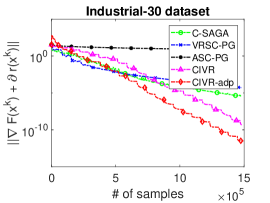
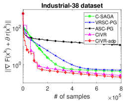
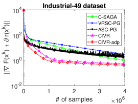
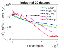
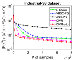
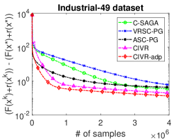
Figure 1: Experiments on the risk-averse portfolio optimization problem.

In this section, we present numerical experiments for a risk-averse portfolio optimization problem. Suppose there are $d$ assets that one can invest during $n$ time periods labeled as $\{1,...,n\}$. Let $R_{i,j}$ be the return or payoff per unit of asset $j$ at time $i$, and $R_{i}$ be the vector consists of $R_{i,1},\ldots,R_{i,d}$. Let $x\in\mathbf{R}^{d}$ be the decision variable, where each component $x_{j}$ represent the amount of investment or percentage of the total investment allocated to asset $j$, for $j=1,\ldots,d$. The same allocations or percentages of allocations are repeated over the $n$ time periods. We would like to maximize the average return over the $n$ periods, but with a penalty on the variance of the returns across the $n$ periods (in other words, we would like different periods to have similar returns).

This problem can be formulated as a finite-sum version of problem (3), with a discrete random variable $\xi\!\in\!\{1,\ldots,n\}$ and $h_{i}(x)\!=\!\langle R_{i},x\rangle$ for $i=1,\ldots,n$. The function $r$ can be chosen as the indicator function of an $\ell_{1}$ ball, or a soft $\ell_{1}$ regularization term. We choose the later one in our experiments to obtain a sparse asset allocation. Using the mappings defined in (4), it can be further transformed into the composite finite-sum problem (2), hence readily solved by the CIVR method. For comparison, we implement the C-SAGA algorithm [34] as a benchmark. As another benchmark, this problem can also be formulated as a two-layer composite finite-sum problem (10), which was done in [12] and [17]. We solve the two-layer formulation by ASC-PG [31] and VRSC-PG [12]. Finally, we also implemented CIVR-adp, which is the adaptive sampling variant described in Theorem 4.

We test these algorithms on three real world portfolio datasets, which contain 30, 38 and 49 industrial portfolios respectively, from the Keneth R. French Data Library. For the three datasets, the daily data of the most recent 24452, 10000 and 24400 days are extracted respectively to conduct the experiments. We set the parameter $\lambda=0.2$ in (3) and use an $\ell_{1}$ regularization $r(x)=0.01\|x\|_{1}$. The experiment results are shown in Figure 1. The curves are averaged over 20 runs and are plotted against the number of samples of the component functions (the horizontal axis).

Throughout the experiments, VRSC-PG and C-SAGA algorithms use the batch size $S=\lceil n^{2/3}\rceil$ while CIVR uses the batch size $S=\lceil\sqrt{n}\rceil$, all dictated by their complexity theory. CIVR-adp employs the adaptive batch size $S_{t}=\bigl{\lceil}\min\{\sqrt{10t+1},\sqrt{n}\}\bigr{\rceil}$ for $t=1,...,T$. For Industrial-30 dataset, all of VRSC-PG, C-SAGA, CIVR and CIVR-adp use the same step size $\eta=0.1$. They are chosen from the set $\eta\in\{1,0.1,0.01,0.001,0.0001\}$ by experiments. And $\eta=0.1$ works best for all four tested methods simultaneously. Similarly, $\eta=0.001$ is chosen for the Industrial-38 dataset and $\eta=0.0001$ is chosen for the Industrial-49 dataset. For ASC-PG, we set its step size parameters $\alpha_{k}=0.001/k$ and $\beta_{k}=1/k$ [see details in 31]. They are hand-tuned to ensure ASC-PG converges fast among a range of tested parameters. Overall, CIVR and CIVR-adp outperform other methods.

Appendices

Appendix A Convergence analysis for composite expectation case

In this section, we focus on convergence analysis of CIVR for solving the stochastic composite optimization problem (1), and prove Theorems 1 and 2.

First, we show that under Assumption 1, the composite function $F(x)=f(g(x))$ is smooth and $F^{\prime}$ has Lipschitz constant $L_{f}=\ell_{g}^{2}L_{f}+\ell_{f}L_{g}$.

$$\left\|F^{\prime}(x)-F^{\prime}(y)\right\| = \left\|g^{\prime}(x)^{T}f^{\prime}(g(x))-g^{\prime}(y)^{T}f^{\prime}(g(y))\right\|$$

$$= \left\|g^{\prime}(x)^{T}f^{\prime}(g(x))-g^{\prime}(x)^{T}f^{\prime}(g(y))+g^{\prime}(x)^{T}f^{\prime}(g(y))-g^{\prime}(y)^{T}f^{\prime}(g(y))\right\|$$

$$\leq \left\|g^{\prime}(x)^{T}f^{\prime}(g(x))-g^{\prime}(x)^{T}f^{\prime}(g(y))\right\|+\left\|g^{\prime}(x)^{T}f^{\prime}(g(y))-g^{\prime}(y)^{T}f^{\prime}(g(y))\right\|$$

$$\leq \left\|g^{\prime}(x)\right\|\left\|f^{\prime}(g(x))-f^{\prime}(g(y))\right\|+\left\|f^{\prime}(g(y))\right\|\left\|g^{\prime}(x)-g^{\prime}(y)\right\|$$

$$\leq \left\|g^{\prime}(x)\right\|\cdot L_{f}\left\|g(x)-g(y)\right\|+\left\|f^{\prime}(g(y))\right\|\cdot L_{g}\left\|x-y\right\|$$

$$\leq \ell_{g}L_{f}\ell_{g}\left\|x-y\right\|+\ell_{f}L_{g}\left\|x-y\right\|$$

$$= \bigl{(}\ell_{g}^{2}L_{f}+\ell_{f}L_{g}\bigr{)}\|x-y\|,$$

where we used $\|g^{\prime}(x)\|\leq\ell_{g}$ and $\|f^{\prime}(g(y))\|\leq\ell_{f}$, which are implied by the Lipschitz conditions on $g$ and $f$ respectively.

Although the incremental estimators used in CIVR are biased, as shown in (19), we can still bound their squared distances from the targets. This is given in the following lemma.

Lemma 1.

Suppose Assumption 1 holds. Let $y_{i}^{t}$ and $z_{i}^{t}$ be constructed according to (11) and (12) in Algorithm 1. For any $t\geq 1$ and $1\leq i\leq\tau_{t}-1$, we have the following mean squared error (MSE) bounds

$$\begin{cases}\displaystyle~{}\mathbf{E}\left[\|y_{i}^{t}-g(x_{i}^{t})\|^{2}\right]\leq\mathbf{E}\left[\|y_{0}^{t}-g(x_{0}^{t})\|^{2}\right]+\sum_{r=1}^{i}\frac{\ell_{g}^{2}}{S_{t}}\mathbf{E}\left[\|x_{r}^{t}-x_{r-1}^{t}\|^{2}\right]\,,\\ \displaystyle~{}\mathbf{E}\left[\|z_{i}^{t}-g^{\prime}(x_{i}^{t})\|^{2}\right]\leq\mathbf{E}\left[\|z_{0}^{t}-g^{\prime}(x_{0}^{k})\|^{2}\right]+\sum_{r=1}^{i}\frac{L_{g}^{2}}{S_{t}}\mathbf{E}\left[\|x_{r}^{t}-x_{r-1}^{t}\|^{2}\right]\,.\end{cases}$$ (33)

Proof.

We first state a fact that allows us to decompose the MSE into a squared bias term and a variance term, that is, for an arbitrary random vector $\zeta$ and a constant vector $u$, we have

$$\mathbf{E}[\|\zeta-u\|^{2}]=\|\mathbf{E}[\zeta]-u\|^{2}+\mathbf{Var}(\zeta),$$ (34)

where $\mathbf{Var}(\zeta):=\mathbf{E}[\|\zeta-\mathbf{E}[\zeta]\|^{2}]$. As a result,

$$\mathbf{E}\left[\|y_{i}^{t}-g(x_{i}^{t})\|^{2}\big{|}x_{i}^{t}\right]=\bigl{\|}\mathbf{E}[y_{i}^{t}|x_{i}^{t}]-g(x_{i}^{t})\bigr{\|}^{2}+\mathbf{Var}\bigl{(}y_{i}^{t}|x_{i}^{t}\bigr{)}.$$

For the bias term, we have $\mathbf{E}[y_{i}^{t}|x_{i}^{t}]-g(x_{i}^{t})=y_{i-1}^{t}-g(x_{i-1}^{t})$. For the variance term, we have

$$\mathbf{Var}\bigl{(}y_{i}^{t}|x_{i}^{t}\bigr{)} = \mathbf{Var}\biggl{(}y_{i-1}^{t}+\frac{1}{S_{t}}\sum_{\xi\in\mathcal{S}_{i}^{t}}(g_{\xi}(x_{i}^{t})-g_{\xi}(x_{i-1}^{t}))\;\Big{|}\;x_{i}^{t}\biggr{)}$$

$$= \frac{1}{S_{t}}\mathbf{Var}\bigl{(}g_{\xi}(x_{i}^{t})-g_{\xi}(x_{i-1}^{t})\;|\,x_{i}^{t}\bigr{)}$$

$$\leq \frac{1}{S_{t}}\mathbf{E}\bigl{[}\|g_{\xi}(x_{i}^{t})-g_{\xi}(x_{i-1}^{t})\|^{2}|x_{i}^{t}\bigr{]}$$

$$\leq \frac{\ell_{g}^{2}}{S_{t}}\|x_{i}^{t}-x_{i-1}^{t}\|^{2},$$

where the second equality is due to the fact that $y_{i-1}^{t}$ is a constant conditioning on $x_{i}^{t}$ and in the last inequality we used the $\ell_{g}$-Lipschitz continuity of $g_{\xi}$. Consequently,

$$\mathbf{E}\left[\|y_{i}^{t}-g(x_{i}^{t})\|^{2}\right]\leq\mathbf{E}\left[\|y_{i-1}^{t}-g(x_{i-1}^{t})\|^{2}\right]+\frac{\ell_{g}^{2}}{S_{t}}\mathbf{E}\left[\|x_{i}^{t}-x_{i-1}^{t}\|^{2}\right].$$

Recursively applying the above procedure yields

$$\mathbf{E}\left[\|y_{i}^{t}-g(x_{i}^{t})\|^{2}\right]\leq\mathbf{E}\left[\|y_{0}^{t}-g(x_{0}^{t})\|^{2}\right]+\sum_{r=1}^{i}\frac{\ell_{g}^{2}}{S_{t}}\mathbf{E}\left[\|x^{t}_{r}-x^{t}_{r-1}\|^{2}\right].$$ (35)

Similarly, the bound on $\mathbf{E}\left[\|z_{i}^{t}-g^{\prime}(x_{i}^{t})\|^{2}\right]$ can be shown by using the $L_{g}$-Lipschitz continuity of $g^{\prime}_{\xi}$. ∎

In Algorithm 1, we approximate the gradient of $F(x):=f(g(x))$ by $\tilde{\nabla}F(x_{i}^{t})=(z_{i}^{t})^{T}f^{\prime}(y_{i}^{t})$. The next lemma bounds the MSE of this estimator.

Lemma 2.

Suppose Assumptions 1 and 2 hold. Then we have

$$\mathbf{E}[\|\tilde{\nabla}F(x_{i}^{t})-F^{\prime}(x_{i}^{t})\|^{2}]\leq\frac{G_{0}}{S_{t}}\sum_{r=1}^{i}\mathbf{E}[\|x_{r}^{t}-x_{r-1}^{t}\|^{2}]+\frac{\sigma_{0}^{2}}{B_{t}},$$ (36)

where

$$G_{0}:=2\bigl{(}\ell_{g}^{4}L_{f}^{2}+\ell_{f}^{2}L_{g}^{2}\bigr{)}\quad\mbox{and}\quad\sigma_{0}^{2}:=2\bigl{(}\ell_{g}^{2}L_{f}^{2}\sigma_{g}^{2}+\ell_{f}^{2}\sigma_{g^{\prime}}^{2}\bigr{)}\,.$$

Proof.

Using Assumption 1, one immediately gets

$$\mathbf{E}\left[\|\tilde{\nabla}F(x_{i}^{t})-F^{\prime}(x_{i}^{t})\|^{2}\right]$$ (37)

$$= \mathbf{E}\left[\|(z_{i}^{t})^{T}f^{\prime}(y_{i}^{t})-(g^{\prime}(x_{i}^{t}))^{T}f^{\prime}(g(x_{i}^{t}))\|^{2}\right]$$

$$= \mathbf{E}\left[\|(z_{i}^{t})^{T}f^{\prime}(y_{i}^{t})-(g^{\prime}(x_{i}^{t}))^{T}f^{\prime}(y_{i}^{t})+(g^{\prime}(x_{i}^{t}))^{T}f^{\prime}(y_{i}^{t})-(g^{\prime}(x_{i}^{t}))^{T}f^{\prime}(g(x_{i}^{t}))\|^{2}\right]$$

$$\leq 2\mathbf{E}\left[\|(z_{i}^{t})^{T}f^{\prime}(y_{i}^{t})-(g^{\prime}(x_{i}^{t}))^{T}f^{\prime}(y_{i}^{t})\|^{2}\right]+2\mathbf{E}\left[\|(g^{\prime}(x_{i}^{t}))^{T}f^{\prime}(y_{i}^{t})-(g^{\prime}(x_{i}^{t}))^{T}f^{\prime}(g(x_{i}^{t}))\|^{2}\right]$$

$$\leq 2\ell_{f}^{2}\mathbf{E}\left[\|z_{i}^{t}-g(x_{i}^{t})\|^{2}\right]+2\ell_{g}^{2}L_{f}^{2}\mathbf{E}\left[\|y_{i}^{t}-g^{\prime}(x_{i}^{t})\|^{2}\right].$$

Therefore, by substituting the MSE bounds provided in Lemma 1 into inequality (37), we obtain

$$\mathbf{E}\left[\|\tilde{\nabla}F(x_{i}^{t})-F^{\prime}(x)\|^{2}\right] \leq \frac{2\bigl{(}\ell_{g}^{4}L_{f}^{2}+\ell_{f}^{2}L_{g}^{2}\bigr{)}}{S_{t}}\sum_{r=1}^{i}\mathbf{E}\left[\|x_{r}^{t}-x_{r-1}^{t}\|^{2}\right]$$ (38)

$$+\;2\ell_{g}^{2}L_{f}^{2}\mathbf{E}\left[\|y_{0}^{t}-g(x_{0}^{t})\|^{2}\right]+2\ell_{f}^{2}\mathbf{E}\left[\|z_{0}^{t}-g^{\prime}(x_{0}^{k})\|^{2}\right].$$

Under Assumption 2, we can bound the MSE of the estimates in (11) as

$$\mathbf{E}\left[\|y_{0}^{t}-g(x_{0}^{t})\|^{2}\right]\leq\frac{\sigma_{g}^{2}}{B_{t}}\,,\qquad\mathbf{E}\left[\|z_{0}^{t}-g^{\prime}(x_{0}^{k})\|^{2}\right]\leq\frac{\sigma_{g^{\prime}}^{2}}{B_{t}}\,.$$

Combining these MSE bounds with (38) yields the desired result. ∎

For the proximal gradient type of algorithms, no matter deterministic or stochastic, a common metric to quantify the optimality of $x_{i}^{t}$ is the norm of the so-called proximal gradient mapping

$$\mathcal{G}_{\eta}(x_{i}^{t}):=\frac{1}{\eta}\bigl{(}x_{i}^{t}-\hat{x}_{i+1}^{t}\bigr{)},$$ (39)

where $\eta$ is the step size used to produce the update

$$\hat{x}_{i+1}^{t}=\mathbf{prox}_{r}^{\eta}\bigl{(}x_{i}^{t}-\eta F^{\prime}(x_{i}^{t})\bigr{)}.$$

Since we use a constant $\eta$ throughout this paper, we will omit the subscript $\eta$ and use $\mathcal{G}(x)$ to denote the proximal gradient mapping at $x$.

Our goal is to find a point $x$ with $\mathbf{E}\bigl{[}\|\mathcal{G}(x)\|^{2}\bigr{]}\leq\epsilon$. However, in Algorithm 1, we only have the approximate proximal gradient mapping

$$\tilde{\mathcal{G}}(x_{i}^{t}):=\frac{1}{\eta}(x_{i}^{t}-x_{i+1}^{t})\,,$$ (40)

where $x_{i+1}^{t}$ is computed using the estimated gradient $\tilde{\nabla}F(x_{i}^{t})$:

$$x_{i+1}^{t}=\mathbf{prox}_{r}^{\eta}\bigl{(}x_{i}^{t}-\eta\tilde{\nabla}F(x_{i}^{t})\bigr{)}.$$

Hence we need to establish the connection between $\mathcal{G}(x_{i}^{t})$ and $\tilde{\mathcal{G}}(x_{i}^{t})$, which is done in the next lemma.

Lemma 3.

For the two gradient mappings defined in (39) and (40), we have

$$\mathbf{E}\left[\|\mathcal{G}(x_{i}^{t})\|^{2}\right]\leq 2\mathbf{E}\left[\|\tilde{\mathcal{G}}(x_{i}^{t})\|^{2}\right]+2\mathbf{E}\left[\|\tilde{\nabla}F(x_{i}^{t})-F^{\prime}(x_{i}^{t})\|^{2}\right].$$ (41)

Proof.

Using the inequality $\|x_{i}^{t}-\hat{x}_{i+1}^{t}\|^{2}\leq 2\|x_{i}^{t}-x_{i+1}^{t}\|^{2}+2\|x_{i+1}^{t}-\hat{x}_{i+1}^{t}\|^{2}$ and the definitions of $\mathcal{G}(x_{i}^{t})$ and $\tilde{\mathcal{G}}(x_{i}^{t})$, we have

$$\mathbf{E}\left[\|\mathcal{G}(x_{i}^{t})\|^{2}\right] \leq 2\mathbf{E}\left[\|\tilde{\mathcal{G}}(x_{i}^{t})\|^{2}\right]+\frac{2}{\eta^{2}}\left\|x_{i+1}^{t}-\hat{x}_{i+1}^{t}\right\|^{2}$$

$$= 2\mathbf{E}\left[\|\tilde{\mathcal{G}}(x_{i}^{t})\|^{2}\right]+\frac{2}{\eta^{2}}\left\|\mathbf{prox}_{r}^{\eta}\bigl{(}x_{i}^{t}-\eta F^{\prime}(x_{i}^{t})\bigr{)}-\mathbf{prox}_{r}^{\eta}\bigl{(}x_{i}^{t}-\eta\tilde{\nabla}F(x_{i}^{t})\bigr{)}\right\|^{2}$$

$$\leq 2\mathbf{E}\left[\|\tilde{\mathcal{G}}(x_{i}^{t})\|^{2}\right]+\frac{2}{\eta^{2}}\left\|x_{i}^{t}-\eta F^{\prime}(x_{i}^{t})-\bigl{(}x_{i}^{t}-\eta\tilde{\nabla}F(x_{i}^{t})\bigr{)}\right\|^{2}$$

$$= 2\mathbf{E}\left[\|\tilde{\mathcal{G}}(x_{i}^{t})\|^{2}\right]+2\mathbf{E}\left[\|\tilde{\nabla}F(x_{i}^{t})-F^{\prime}(x_{i}^{t})\|^{2}\right],$$

where in the second inequality we used the non-expansive property of proximal mapping [e.g., 26, Section 31]. ∎

The next lemma bounds the amount of expected descent per iteration in Algorithm 1.

Lemma 4.

Let the sequence $\{x_{i}^{t}\}$ be generated by Algorithm 1. Then for all $t\geq 1$ and $0\leq i\leq\tau_{t}-1$, we have the following two inequalities

$$\mathbf{E}[\Phi(x_{i+1}^{t})]~{}\leq~{}\mathbf{E}[\Phi(x_{i}^{t})]-\left(\frac{\eta}{2}-\frac{L_{F}\eta^{2}}{2}\right)\mathbf{E}\left[\|\tilde{\mathcal{G}}(x_{i}^{t})\|^{2}\right]+\frac{\eta}{2}\mathbf{E}[\|\tilde{\nabla}F(x_{i}^{t})-F^{\prime}(x_{i}^{t})\|^{2}],$$ (42)

and

$$\mathbf{E}[\Phi(x_{i+1}^{t})]~{}\leq~{} \mathbf{E}[\Phi(x_{i}^{t})]-\frac{\eta}{8}\mathbf{E}[\|\mathcal{G}(x_{i}^{t})\|^{2}]+\frac{3\eta}{4}\mathbf{E}[\|\tilde{\nabla}F(x_{i}^{t})-F^{\prime}(x_{i}^{t})\|^{2}]$$

$$-\left(\frac{1}{4\eta}-\frac{L_{F}}{2}\right)\mathbf{E}\left[\|x_{i}^{t}-x_{i+1}^{t}\|^{2}\right].$$ (43)

Proof.

By applying the $L_{F}$-Lipschitz continuity of $F^{\prime}$ and the optimality of the $\frac{1}{\eta}$-strongly convex subproblem, we have

$$\Phi(x_{i+1}^{t}) = F(x_{i+1}^{t})+r(x_{i+1}^{t})$$

$$\leq F(x_{i}^{t})+\langle F^{\prime}(x_{i}^{t}),x_{i+1}^{t}-x_{i}^{t}\rangle+\frac{L_{F}}{2}\|x_{i+1}^{t}-x_{i}^{t}\|^{2}+r(x_{i+1}^{t})$$

$$= F(x_{i}^{t})+\langle\tilde{\nabla}F(x_{i}^{t}),x_{i+1}^{t}-x_{i}^{t}\rangle+\frac{1}{2\eta}\|x_{i+1}^{t}-x_{i}^{t}\|^{2}+r(x_{i+1}^{t})$$

$$+\langle F^{\prime}(x_{i}^{t})-\tilde{\nabla}F(x_{i}^{t}),x_{i+1}^{t}-x_{i}^{t}\rangle-(\frac{1}{2\eta}-\frac{L_{F}}{2})\|x_{i+1}^{t}-x_{i}^{t}\|^{2}$$

$$\leq F(x_{i}^{t})+r(x_{i}^{t})-\frac{1}{2\eta}\|x_{i+1}^{t}-x_{i}^{t}\|^{2}-(\frac{1}{2\eta}-\frac{L_{F}}{2})\|x_{i+1}^{t}-x_{i}^{t}\|^{2}$$

$$+\frac{\eta}{2}\|\tilde{\nabla}F(x_{i}^{t})-F^{\prime}(x_{i}^{t})\|^{2}+\frac{1}{2\eta}\|x_{i+1}^{t}-x_{i}^{t}\|^{2}$$

$$= \Phi(x_{i}^{t})-(\frac{1}{2\eta}-\frac{L_{F}}{2})\|x_{i+1}^{t}-x_{i}^{t}\|^{2}+\frac{\eta}{2}\|\tilde{\nabla}F(x_{i}^{t})-F^{\prime}(x_{i}^{t})\|^{2}.$$

Taking the expectation on both sides completes the proof of inequality (42). By inequality (41), we know that

$$-\frac{\eta}{4}\mathbf{E}[\|\tilde{\mathcal{G}}(x_{i}^{t})\|^{2}]\leq-\frac{\eta}{8}\mathbf{E}[\|\mathcal{G}(x_{i}^{t})\|^{2}]+\frac{\eta}{4}\mathbf{E}[\|\tilde{\nabla}F(x_{i}^{t})-F^{\prime}(x_{i}^{t})\|^{2}].$$

Adding this inequality in to (42) yields (43). ∎

A.1 Proof of Theorem 1

Proof.

Because all $\tau_{t}$, $B_{t}$ and $S_{t}$ are taking their values independent of $t$. We denote $\tau=\tau_{t}$, $B=B_{t}$ and $S=S_{t}$ for all $t$ for clarity. By Lemma 4, summing up inequality (43) throughout the $t$-th epoch and applying (36) gives

$$\frac{\eta}{8}\sum_{i=0}^{\tau-1}\mathbf{E}[\|\mathcal{G}(x_{i}^{t})\|^{2}] \leq \mathbf{E}[\Phi(x_{0}^{t})]-\mathbf{E}[\Phi(x_{\tau}^{t})]-\left(\frac{1}{4\eta}-\frac{L_{F}}{2}\right)\sum_{r=1}^{\tau}\mathbf{E}[\|x_{r}^{t}-x_{r-1}^{t}\|^{2}]$$

$$+\frac{3G_{0}\eta}{4S}\sum_{i=1}^{\tau-1}\sum_{r=1}^{i}\mathbf{E}[\|x_{r}^{t}-x_{r-1}^{t}\|^{2}]+\frac{3\sigma_{0}^{2}\eta}{4B}\tau$$

$$\leq \mathbf{E}[\Phi(x_{0}^{t})]-\mathbf{E}[\Phi(x_{\tau}^{t})]-\left(\frac{1}{4\eta}-\frac{L_{F}}{2}-\tau\frac{3G_{0}\eta}{4S}\right)\sum_{r=1}^{\tau}\mathbf{E}[\|x_{r}^{t}-x_{r-1}^{t}\|^{2}]$$

$$+\frac{3\sigma_{0}^{2}\eta}{4B}\tau,$$

where the second inequality is due to the fact that

$$\sum_{i=1}^{\tau-1}\sum_{r=1}^{i}\mathbf{E}[\|x_{r}^{t}-x_{r-1}^{t}\|^{2}]\leq\tau\sum_{r=1}^{\tau}\mathbf{E}[\|x_{r}^{t}-x_{r-1}^{t}\|^{2}].$$

When we choose the parameters satisfying $\tau\leq S$, then the coefficient $\frac{1}{4\eta}-\frac{L_{F}}{2}-\tau\frac{3G_{0}\eta}{4S}\geq\frac{1}{4\eta}-\frac{L_{F}}{2}-\frac{3G_{0}\eta}{4}$ which depends only on the parameter $\eta$ and some constant. If we choose the $\eta$ according to the theorem, then $\frac{1}{4\eta}-\frac{L_{F}}{2}-\frac{3G_{0}\eta}{4}\geq 0$, yielding that

$$\frac{\eta}{8}\sum_{i=0}^{\tau-1}\mathbf{E}[\|\mathcal{G}(x_{i}^{t})\|^{2}]~{}\leq~{}\mathbf{E}[\Phi(x_{0}^{t})]-\mathbf{E}[\Phi(x_{\tau}^{t})]+\frac{3\sigma_{0}^{2}\eta}{4B}\tau.$$ (44)

Summing this up throughout the epochs gives

$$\frac{\eta}{8}\sum_{t=1}^{T}\sum_{i=0}^{\tau-1}\mathbf{E}[\|\mathcal{G}(x_{i}^{t})\|^{2}]~{}\leq~{}\mathbf{E}[\Phi(x_{0}^{1})]-\mathbf{E}[\Phi(x_{\tau}^{T})]+\frac{3\sigma_{0}^{2}\eta}{4B}\tau T\leq\Phi(x_{0}^{1})-\Phi^{*}+\frac{3\sigma_{0}^{2}\eta}{4B}\tau T,$$

where we have applied the fact that $x_{0}^{t}=x_{\tau}^{t-1}$. By the random sampling scheme for output $\bar{x}$, we have

$$\mathbf{E}[\|\mathcal{G}(\bar{x})\|^{2}]=\frac{1}{\tau T}\sum_{t=1}^{T}\sum_{i=0}^{\tau-1}\mathbf{E}[\|\mathcal{G}(x_{i}^{t})\|^{2}]\leq\frac{8(\Phi(x_{0}^{1})-\Phi^{*})}{\tau T\eta}+\frac{6\sigma_{0}^{2}}{B}.$$ (45)

Substitute the values of $T,\tau$ and $B$ gives (22). ∎

To simplify presentation, we omit $\lceil\cdot\rceil$ on integer parameters in the following discussion.

• With $\eta\leq\frac{4}{L_{F}+\sqrt{L_{F}^{2}+12G_{0}}}$, and letting $T=1/\sqrt{\epsilon}$, $B=\sigma_{0}^{2}/\epsilon$, and $\tau=S=1/\sqrt{\epsilon}$, we have

  $$\mathbf{E}[\|\mathcal{G}(\bar{x})\|^{2}]\leq 8\bigl{(}(\Phi(x_{0}^{1})-\Phi^{*})\eta^{-1}+6\bigr{)}\epsilon,$$

  and the sample complexity is $T(B+2\tau S)={\mathcal{O}}\bigl{(}\sigma_{0}^{2}\epsilon^{-3/2}+\epsilon^{-3/2}\bigr{)}$, as in our theorem.

• With $\eta\leq\frac{4}{L_{F}+\sqrt{L_{F}^{2}+12G_{0}}}$, and letting $T=1/\epsilon$, $B=1+\sigma_{0}^{2}/\epsilon$, and $\tau=S=1$, we again obtain

  $$\mathbf{E}[\|\mathcal{G}(\bar{x})\|^{2}]\leq 8\bigl{(}(\Phi(x_{0}^{1})-\Phi^{*})\eta^{-1}+6\bigr{)}\epsilon,$$

  but the sample complexity is $T(B+2\tau S)={\mathcal{O}}\bigl{(}\sigma_{0}^{2}\epsilon^{-2}+\epsilon^{-1}\bigr{)}$, which is same as in Ghadimi and Lan [9]. For deterministic optimization with $\sigma_{0}=0$, this recovers the ${\mathcal{O}}(\epsilon^{-1})$ complexity.

A.2 Proof of Theorem 2

Proof.

Note that for this set of parameters, we still have the relationship that $\tau_{t}=S_{t}$. Therefore, within each epoch, (44) is still true with epoch specific $\tau_{t}$ and $B_{t}$. Summing this up gives

$$\frac{\eta}{8}\sum_{t=1}^{T}\sum_{i=0}^{\tau_{t}-1}\mathbf{E}[\|\mathcal{G}(x_{i}^{t})\|^{2}]\leq\Phi(x_{0}^{1})-\Phi^{*}+\sum_{t=1}^{T}\frac{3\sigma_{0}^{2}\eta}{4B_{t}}\tau_{t}.$$ (46)

By the random selection rule of $\bar{x}$, we have

$$\mathbf{E}[\|\mathcal{G}(\bar{x})\|^{2}]=\frac{1}{\sum_{t=1}^{T}\tau_{t}}\sum_{t=1}^{T}\sum_{i=0}^{\tau-1}\mathbf{E}[\|\mathcal{G}(x_{i}^{t})\|^{2}]\leq\frac{8(\Phi(x_{0}^{1})-\Phi^{*})}{\eta\sum_{t=1}^{T}\tau_{t}}+6\sigma_{0}^{2}\cdot\frac{\sum_{t=1}^{T}\tau_{t}/B_{t}}{\sum_{t=1}^{T}\tau_{t}}.$$ (47)

Note that $\tau_{t}=\lceil at+b\rceil$ and $B_{t}=\lceil\sigma_{0}^{2}(at+b)^{2}\rceil.$ We have

$$\sum_{t=1}^{T}\tau_{t}\geq\sum_{t=1}^{T}at+b=\frac{a}{2}T(T+1)+bT={\mathcal{O}}(T^{2})$$

and

$$\sigma_{0}^{2}\sum_{t=1}^{T}\tau_{t}/B_{t}\leq\sum_{t=1}^{T}\frac{1}{at+b}\leq\frac{1}{a+b}+\int_{1}^{T}\frac{dt}{at+b}=\frac{1}{a+b}+\frac{1}{a}\ln\left(\frac{aT+b}{a+b}\right)={\mathcal{O}}(\ln T).$$

Substituting the above bounds into inequality (47) gives (23). As a result, the total sample complexity is

$$\sum_{t=1}^{T}\bigl{(}B_{t}+2\tau_{t}S_{t}\bigr{)}\leq\sum_{t=1}^{T}\left(\sigma_{0}^{2}(at+b)^{2}+2(at+b)^{2}\right)={\mathcal{O}}(\sigma_{0}^{2}T^{3}+T^{3})\,.$$

Setting $T=\tilde{{\mathcal{O}}}(\epsilon^{-1/2})$ so that $\mathbf{E}[\|\mathcal{G}\|\bar{x}\|^{2}]\leq\epsilon$, we get sample complexity $\tilde{{\mathcal{O}}}(\sigma_{0}^{2}\epsilon^{-3/2}+\epsilon^{-3/2})$. ∎

We can also choose a different set of parameters. With $\eta\leq\frac{4}{L_{F}+\sqrt{L_{F}^{2}+12G_{0}}}$, and letting $B=1+\sigma_{0}^{2}(at+b)$, and $\tau=S=1$, we also have

$$\mathbf{E}[\|\mathcal{G}(\bar{x})\|^{2}]\leq\frac{8(\Phi(x_{0}^{1})-\Phi^{*})}{\eta T}+\frac{6\ln T}{T}\,,$$

but the sample complexity, by setting $T=\tilde{{\mathcal{O}}}(\epsilon^{-1})$ so that the above bound is less than $\epsilon$, is

$$\sum_{t=1}^{T}\bigl{(}B_{t}+2\tau_{t}S_{t}\bigr{)}\leq\sum_{t=1}^{T}\left(\sigma_{0}^{2}(at+b)+2\right)={\mathcal{O}}(\sigma_{0}^{2}T^{2}+T)=\tilde{{\mathcal{O}}}(\sigma_{0}^{2}\epsilon^{-2}+\epsilon^{-1})\,.$$

This is more close to the classical results on stochastic optimization.

Appendix B Convergence analysis for composite finite-sum case

In this section, we consider the composite finite-sum problem (2) and prove Theorems 3 and 4.

In this case, the random variable $\xi$ uniformly takes value from the finite index set $\{1,...,n\}$. At the beginning of each epoch in Algorithm 1, we can choose to estimate $g(x_{0}^{t})^{t}$ and $g^{\prime}(x_{0}^{t})$ by their exact value rather than the approximate ones constructed by subsampling. Namely, in (11) of Algorithm 1, we choose $\mathcal{B}_{t}=\{1,\ldots,n\}$ for all $t\geq 1$. Therefore,

$$y_{0}^{t}=g(x_{0}^{t})=\frac{1}{n}\sum_{j=1}^{n}g_{j}(x_{0}^{t}),\qquad z_{0}^{t}=g^{\prime}(x_{0}^{t})=\frac{1}{n}\sum_{j=1}^{n}g^{\prime}_{j}(x_{0}^{t})$$

and

$$\mathbf{E}\left[\|y_{0}^{t}-g(x_{0}^{t})\|^{2}\right]=0\,,\qquad\mathbf{E}\left[\|z_{0}^{t}-g^{\prime}(x_{0}^{k})\|^{2}\right]=0\,.$$ (48)

As a result, the initial variances in Lemma 1 diminishes and (33) reduces to

$$\begin{cases}\displaystyle\mathbf{E}[\|y_{i}^{t}-g(x_{i}^{t})\|^{2}]\leq\sum_{r=1}^{i}\frac{\ell_{g}^{2}}{S_{t}}\mathbf{E}[\|x_{r}^{t}-x_{r-1}^{t}\|^{2}],\\ \displaystyle\mathbf{E}[\|z_{i}^{t}-g^{\prime}(x_{i}^{t})\|^{2}]\leq\sum_{r=1}^{i}\frac{L_{g}^{2}}{S_{t}}\mathbf{E}[\|x_{r}^{t}-x_{r-1}^{t}\|^{2}].\end{cases}$$ (49)

In addition, combining (38) and (48), we have

$$\mathbf{E}[\|\tilde{\nabla}F(x_{i}^{t})-F^{\prime}(x)\|^{2}]\leq\frac{G_{0}}{S_{t}}\sum_{r=1}^{i}\mathbf{E}[\|x_{r}^{t}-x_{r-1}^{t}\|^{2}].$$ (50)

Note that Lemma 4 is still true.

B.1 Proof of Theorem 3

Proof.

The proof follows similar steps as those in the proof of Theorem 1. So we only note down the significantly different steps here.

Specifically, following the proof of Theorem 1 in Section A.1, by applying (49) instead of (33), we get the following result instead of inequality (44),

$$\frac{\eta}{8}\sum_{i=0}^{\tau-1}\mathbf{E}[\|\mathcal{G}(x_{i}^{t})\|^{2}]\leq\mathbf{E}[\Phi(x_{0}^{t})]-\mathbf{E}[\Phi(x_{\tau}^{t})].$$

Summing this up apply the random selection rule of $\bar{x}$ gives

$$\mathbf{E}[\|\mathcal{G}(\bar{x})\|^{2}]=\frac{1}{\tau T}\sum_{t=1}^{T}\sum_{i=0}^{\tau-1}\mathbf{E}[\|\mathcal{G}(x_{i}^{t})\|^{2}]\leq\frac{8(\Phi(x_{0}^{1})-\Phi^{*})}{\tau T\eta}=\frac{8(\Phi(x_{0}^{1})-\Phi^{*})}{\sqrt{n}T\eta}.$$

Therefore, we have to set $T={\mathcal{O}}(\frac{1}{\sqrt{n}\epsilon})$ to get an $\epsilon$-solution. Note that the sample complexity per epoch is $n+\tau_{t}S_{t}=2n$, the total sample complexity will be ${\mathcal{O}}(n+\sqrt{n}\epsilon^{-1})$. ∎

B.2 Proof of Theorem 4

Proof.

If $T\leq T_{0}$, then the result is exactly what we proved from Theorem 2. Therefore, the first bound in (26) is already guaranteed.

If $T>T_{0}$, when $1\leq t\leq T_{0}$, then everything still runs identically to that described in Theorem 2. Consequently, the following bound is effective

$$\frac{\eta}{8}\sum_{t=1}^{T_{0}}\sum_{i=0}^{\tau_{t}-1}\mathbf{E}[\|\mathcal{G}(x_{i}^{t})\|^{2}]\leq\Phi(x_{0}^{1})-\mathbf{E}[\Phi(x^{T_{0}+1}_{0})]+\sum_{t=1}^{T_{0}}\frac{3\sigma_{0}^{2}\eta}{4B_{t}}\tau_{t}.$$ (51)

When $T_{0}+1\leq t\leq T$, the following bound becomes effective,

$$\frac{\eta}{8}\sum_{t=T_{0}+1}^{T}\sum_{i=0}^{\tau-1}\mathbf{E}[\|\mathcal{G}(x_{i}^{t})\|^{2}]\leq\mathbf{E}[\Phi(x_{0}^{T_{0}+1})]-\Phi^{*}.$$

Therefore, we have

$$\mathbf{E}[\|\mathcal{G}(\bar{x})\|^{2}]=\frac{1}{\sum_{t=1}^{T}\tau_{t}}\sum_{t=1}^{T}\sum_{i=0}^{\tau-1}\mathbf{E}[\|\mathcal{G}(x_{i}^{t})\|^{2}]\leq\frac{8(\Phi(x_{0}^{1})-\Phi^{*})}{\eta\sum_{t=1}^{T}\tau_{t}}+6\sigma_{0}^{2}\cdot\frac{\sum_{t=1}^{T_{0}}\tau_{t}/B_{t}}{\sum_{t=1}^{T}\tau_{t}}.$$

Note that

$$\sum_{t=1}^{T_{0}}\tau_{t}/B_{t}\leq\sum_{t=1}^{T_{0}}\frac{1}{at+b}\leq\frac{1}{a+b}+\frac{1}{a}\ln\left(\frac{aT_{0}+b}{a+b}\right)={\mathcal{O}}(\ln n),$$

and

$$\sum_{t=1}^{T}\tau_{t}\geq(T-T_{0})\sqrt{n}+\sum_{t=1}^{T_{0}}(at+b)=\sqrt{n}(T-T_{0})+\frac{a}{2}T^{2}_{0}+(\frac{a}{2}+b)T_{0}={\mathcal{O}}(\sqrt{n}(T-T_{0}+1)).$$

With the above two bounds, we have proved the second result in (26).

For any $\epsilon>0$, if $\epsilon\geq{\mathcal{O}}(1/T_{0}^{2})={\mathcal{O}}(n^{-1}).$ In this case, the algorithm will spend most epochs in the adaptive phase, whose sample complexity is $\tilde{{\mathcal{O}}}(\epsilon^{-3/2})$. if $\epsilon=o(n^{-1})$, we need $T>T_{0}$. By (26), we know $\sqrt{n}(T-T_{0}+1)=\tilde{\mathcal{O}}(\epsilon^{-1})$, this means that the total sample complexity will be

$$\sum_{t=1}^{T}\bigl{(}B_{t}+2\tau_{t}S_{t}\bigr{)}\leq 3\sum_{t=1}^{T_{0}}(at+b+1)^{2}+3(T-T_{0})n=\tilde{\mathcal{O}}(n^{3/2}+\sqrt{n}\epsilon^{-1})=\tilde{{\mathcal{O}}}(\sqrt{n}\epsilon^{-1}).$$

When $\epsilon\geq{\mathcal{O}}(n^{-1})$, we have $\epsilon^{-3/2}\leq\sqrt{n}\epsilon^{-1}$. When $\epsilon=o(n^{-1})$, we have $\epsilon^{-3/2}>\sqrt{n}\epsilon^{-1}$. Combining the two cases together gives the sample complexity of $\tilde{{\mathcal{O}}}(\min\{\sqrt{n}\epsilon^{-1},\epsilon^{-3/2}\})$. ∎

Appendix C Convergence analysis under gradient-dominant condition

C.1 Proof of Theorem 5

Proof.

Note that in this case $\Phi(x)=F(x)$. By (45) and (27), we have

$$\mathbf{E}[F(\bar{x})-F^{*}]\leq\nu\mathbf{E}[\|F^{\prime}(\bar{x})\|^{2}]\leq\frac{8\nu(F(x_{0}^{1})-F^{*})}{\tau T\eta}+\frac{6\nu\sigma_{0}^{2}}{B}$$

By the selection of $T=\bigl{\lceil}\frac{16\nu\sqrt{\epsilon}}{\eta}\bigr{\rceil}$, $\tau=1/\sqrt{\epsilon}$ and $B=1+12\nu\sigma_{0}^{2}/\epsilon$, we have

$$\mathbf{E}[F(\bar{x})-F^{*}]\leq\frac{1}{2}(F(x_{0}^{1})-F^{*})+\frac{1}{2}\epsilon,$$ (52)

which is (28).

Suppose we periodically restart the Algorithm 1 after every $T$epochs, and set the outputs to be $\bar{x}^{k}$, where $k=1,2,...$ denotes the number of restarts. We use the output of the $k$th period $\bar{x}^{k}$ as the initial point to start the next period, which produces $\bar{x}^{k+1}$. As a result, the above inequality translates to

$$\mathbf{E}[F(\bar{x}^{k+1})-F^{*}]\leq\frac{1}{2}(\mathbf{E}[F(\bar{x}^{k})]-F^{*})+\frac{1}{2}\epsilon.$$

Equivalently,

$$\mathbf{E}[F(\bar{x}^{k})-F^{*}]-\epsilon\leq\frac{1}{2}\left(\mathbf{E}[F(\bar{x}^{k-1})-F^{*}]-\epsilon\right),$$

which leads to

$$\mathbf{E}[F(\bar{x}^{k})-F^{*}]\leq\frac{1}{2^{k}}\left(\mathbf{E}[F(\bar{x}^{0})-F^{*}]-\epsilon\right)+\epsilon.$$

Therefore, the expected optimality gap converges linearly to a $\epsilon$-ball around 0. ∎

Next we discuss the sample complexity with different parameter settings.

• If we choose $\tau=S=1/\sqrt{\epsilon}$, $B_{t}=12\nu\sigma_{0}^{2}/\epsilon$, and $T=\bigl{\lceil}\frac{16\nu\sqrt{\epsilon}}{\eta}\bigr{\rceil}$, then the total sample complexity is

  $$T(B+2\tau S)\ln\frac{1}{\epsilon}=\frac{16\nu\sqrt{\epsilon}}{\eta}\left(\frac{12\nu\sigma_{0}^{2}}{\epsilon}+\frac{1}{\sqrt{\epsilon}}\frac{1}{\sqrt{\epsilon}}\right)\ln\frac{1}{\epsilon}={\mathcal{O}}\left((\nu^{2}\sigma_{0}^{2}\epsilon^{-1/2}+\nu\epsilon^{-1/2})\ln\epsilon^{-1}\right)$$

  However, the above derivation needs to assume $\frac{16\nu\sqrt{\epsilon}}{\eta}\geq 1$ or at least ${\mathcal{O}}(1)$, which means $\epsilon>(\eta/\nu)^{2}$. If this condition is not satisfied, then we have $T=1$ and the complexity is

  $${\mathcal{O}}\bigl{(}(\nu\sigma_{0}^{2}\epsilon^{-1}+\epsilon^{-1})\ln\epsilon^{-1}\bigr{)}.$$

  Notice that the second term does not depend on $\nu$ or the conditions number.

• If we choose $\tau=S=1$, $B_{t}=1+12\nu\sigma_{0}^{2}/\epsilon$, and $T=\bigl{\lceil}\frac{16\nu}{\eta}\bigr{\rceil}$, the we also have

  $$\mathbf{E}[F(\bar{x})-F^{*}]\leq\frac{1}{2}(F(x_{0}^{1})-F^{*})+\frac{1}{2}\epsilon,$$

  and the total sample complexity is

  $$T(B+2\tau S)\ln\frac{1}{\epsilon}=\frac{16\nu}{\eta}\left(\frac{12\nu\sigma_{0}^{2}}{\epsilon}+2\right)\ln\frac{1}{\epsilon}={\mathcal{O}}\left(\nu^{2}\sigma_{0}^{2}\epsilon^{-1/2}+\nu\right)\ln\epsilon^{-1}$$

  Defining the condition number $\kappa=L_{F}\nu={\mathcal{O}}(\nu/\eta)$, the above complexity becomes

  $$T(B+2\tau S)\ln\frac{1}{\epsilon}={\mathcal{O}}\left(\kappa^{2}\sigma_{0}^{2}\epsilon^{-1}+\kappa\right)\ln\epsilon^{-1}$$

  Thus when $\sigma=0$, we have ${\mathcal{O}}\bigl{(}\kappa\ln\epsilon^{-1}\bigr{)}$ for deterministic optimization.

C.2 Proof of Theorem 6

The proof is very similar to the previous one. It actually becomes simpler by noticing that in the finite-sum case, the terms involving $\sigma_{0}^{2}$ disappear:

$$\mathbf{E}[F(\bar{x})-F^{*}]\leq\nu\mathbf{E}[\|F^{\prime}(\bar{x})\|^{2}]\leq\frac{8\nu(F(x_{0}^{1})-F^{*})}{\tau T\eta}.$$

By choosing $T=\bigl{\lceil}\frac{16\nu}{\eta\sqrt{n}}\bigr{\rceil}$, $\tau=S=\sqrt{n}$. we again obtain (52). In this case, we have $B=n$ and

$$T(B+2\tau S)\epsilon^{-1}=\left\lceil\frac{16\nu}{\eta\sqrt{n}}\right\rceil\left(n+2\sqrt{n}\sqrt{n}\right)\ln\epsilon^{-1}={\mathcal{O}}\left(n+\nu\sqrt{n}\right)\ln\epsilon^{-1}.$$

Appendix D Convergence analysis under optimally strong convexity

In order to prove Theorems 7 and 8, we first state Lemma 3 in [33] in our notations.

Lemma 5 (Lemma 3 in [33]).

Let $\Phi(x)=F(x)+r(x)$, where $F^{\prime}(x)$ is $L_{F}$-Lipschitz continuous, and $F(x)$ and $r(x)$ are convex. For any $x\in\mathrm{dom}(r)$, and any $v\in\mathbf{R}^{d}$, define

$$x^{+}:=\mathrm{Prox}_{\eta r(\cdot)}(x-\eta v),\mbox{ }\mathcal{G}:=\frac{1}{\eta}(x-x^{+}),\mbox{ and }\Delta:=v-F^{\prime}(x),$$

where $\eta$ is a step size satisfying $0<\eta\leq 1/L_{F}$. Then for any $y\in\mathbf{R}^{d}$,

$$\Phi(y)\geq\Phi(x^{+})+\mathcal{G}^{T}(y-x)+\frac{\eta}{2}\|\mathcal{G}\|^{2}+\Delta^{T}(x^{+}-y).$$

D.1 Proof of Theorem 7

Proof.

If we set $x=x_{i}^{t}$, $y=x^{*}$, $v=\tilde{\nabla}F(x_{i}^{t})$, $x^{+}=x_{i+1}^{t}$ and $\mathcal{G}=\tilde{\mathcal{G}}(x_{i}^{t})$, we get the following useful inequality,

$$\langle\tilde{\mathcal{G}}(x_{i}^{t}),x^{*}-x_{i}^{t}\rangle\leq\Phi(x^{*})-\Phi(x_{i+1}^{t})-\frac{\eta}{2}\|\tilde{\mathcal{G}}(x_{i}^{t})\|^{2}-\langle F^{\prime}(x_{i}^{t})-\tilde{\nabla}F(x_{i}^{t}),x^{*}-x_{i+1}^{t}\rangle.$$

As a result we have the following inequality,

$$\|x_{i+1}^{t}-x^{*}\|^{2}$$ (53)

$$= \|x_{i}^{t}-x^{*}\|^{2}+\eta^{2}\|\tilde{\mathcal{G}}(x_{i}^{t})\|^{2}+2\eta\langle\tilde{\mathcal{G}}(x_{i}^{t}),x^{*}-x_{i}^{t}\rangle$$

$$\leq \|x_{i}^{t}-x^{*}\|^{2}+\eta^{2}\|\tilde{\mathcal{G}}(x_{i}^{t})\|^{2}-2\eta(\Phi(x_{i+1}^{t})-\Phi(x^{*}))-\eta^{2}\|\tilde{\mathcal{G}}(x_{i}^{t})\|^{2}$$

$$-2\eta\langle F^{\prime}(x_{i}^{t})-\tilde{\nabla}F(x_{i}^{t}),x^{*}-x_{i+1}^{t}\rangle$$

$$\leq \|x_{i}^{t}-x^{*}\|^{2}-2\eta(\Phi(x_{i+1}^{t})-\Phi(x^{*}))+\frac{2\eta}{\mu}\|F^{\prime}(x_{i}^{t})-\tilde{\nabla}F(x_{i}^{t})\|^{2}+\frac{\eta\mu}{2}\|x_{i+1}^{t}-x^{*}\|^{2}$$

$$\leq \|x_{i}^{t}-x^{*}\|^{2}-\eta(\Phi(x_{i+1}^{t})-\Phi(x^{*}))+\frac{2\eta}{\mu}\|F^{\prime}(x_{i}^{t})-\tilde{\nabla}F(x_{i}^{t})\|^{2}.$$

Note that the inequality (53) is originally obtained in [34]. Adding $2\mu\cdot$(53) to (42), we get

$$2\mu\eta\mathbf{E}[\Phi(x_{i+1}^{t})-\Phi^{*}] \leq \mathbf{E}[\Phi(x_{i}^{t})+2\mu\|x_{i}^{t}-x^{*}\|^{2}]-\mathbf{E}[\Phi(x_{i+1}^{t})+2\mu\|x_{i+1}^{t}-x^{*}\|^{2}]$$ (54)

$$-(\frac{1}{2\eta}-\frac{L_{F}}{2})\mathbf{E}[\|x_{i+1}^{t}-x_{i}^{t}\|^{2}]+\frac{9}{2}\eta\mathbf{E}[\|\tilde{\nabla}F(x_{i}^{t})-F^{\prime}(x_{i}^{t})\|^{2}].$$

By (54) and (36), we have

$$2\mu\eta\sum_{i=0}^{\tau_{t}-1}\mathbf{E}[\Phi(x_{i+1}^{t})-\Phi^{*}] \leq \mathbf{E}[\Phi(x_{\tau_{t}}^{t})+2\mu\|x_{\tau_{t}}^{t}-x^{*}\|^{2}]-\mathbf{E}[\Phi(x_{0}^{t})+2\mu\|x_{0}^{t}-x^{*}\|^{2}]$$

$$-(\frac{1}{2\eta}-\frac{L_{F}}{2}-\tau_{t}\frac{9G_{0}\eta}{2S_{t}})\sum_{r=1}^{\tau_{t}}\mathbf{E}[\|x_{r}^{t}-x_{r-1}^{t}\|^{2}]+\tau_{t}\frac{9\sigma_{0}^{2}\eta}{2B_{t}}.$$

According to the selection of $\tau_{t},S_{t},B_{t}$ and $\eta$, we know that the coefficient $(\frac{1}{2\eta}-\frac{L_{F}}{2}-\tau_{t}\frac{9G_{0}\eta}{2S_{t}})\geq 0$. Consequently,

$$2\mu\eta\sum_{i=0}^{\tau_{t}-1}\mathbf{E}[\Phi(x_{i+1}^{t})-\Phi^{*}] \leq \mathbf{E}[\Phi(x_{\tau_{t}}^{t})+2\mu\|x_{\tau_{t}}^{t}-x^{*}\|^{2}]-\mathbf{E}[\Phi(x_{0}^{t})+2\mu\|x_{0}^{t}-x^{*}\|^{2}]+\tau_{t}\frac{9\sigma_{0}^{2}\eta}{2B_{t}}.$$

Summing this up and apply the random selection rule of $\bar{x}$ gives

$$\mathbf{E}[\Phi(\bar{x})-\Phi^{*}] \leq \frac{1}{2\mu\eta\tau T}\mathbf{E}[\Phi(x_{0}^{1})-\Phi^{*}+2\mu\|x_{0}^{1}-x^{*}\|^{2}]+\frac{9\sigma_{0}^{2}}{4\mu B_{t}}$$

$$\leq \frac{5}{2\mu\eta\tau T}\mathbf{E}[\Phi(x_{0}^{1})-\Phi^{*}]+\frac{9\sigma_{0}^{2}}{4\mu B_{t}}\,.$$

If we choose $T=\lceil\frac{5\sqrt{\epsilon}}{\mu\eta}\rceil$, $\tau=S=\frac{1}{\sqrt{\epsilon}}$ and $B_{t}=1+\frac{9\sigma_{0}^{2}}{2\mu\epsilon}$, then $\frac{5}{2\mu\eta\tau T}\leq\frac{1}{2}$ and we obtain

$$\mathbf{E}[\Phi(\bar{x})-\Phi^{*}]~{}\leq~{}\frac{1}{2}\mathbf{E}[\Phi(x_{0}^{1})-\Phi^{*}]+\frac{1}{2}\epsilon\,.$$

This proves the inequality (31). The rest of the proof will mimic that of Theorem 5. ∎

Discussions on sample complexity:

• If we choose $\tau=S=1/\sqrt{\epsilon}$, $B_{t}=1+\frac{9\sigma_{0}^{2}}{2\mu\epsilon}$, and $T=\lceil\frac{5\sqrt{\epsilon}}{\mu\eta}\rceil$, then the sample complexity is

  $$T(B+2\tau S)\ln\frac{1}{\epsilon}=\frac{5\sqrt{\epsilon}}{\mu\eta}\left(\frac{9\sigma_{0}^{2}}{2\mu\epsilon}+\frac{1}{\sqrt{\epsilon}}\frac{1}{\sqrt{\epsilon}}\right)\ln\frac{1}{\epsilon}={\mathcal{O}}\left((\mu^{-2}\sigma_{0}^{2}\epsilon^{-1/2}+\mu^{-1}\epsilon^{-1/2})\ln\epsilon^{-1}\right)\,.$$

  The above derivation needs to assume $\frac{5\sqrt{\epsilon}}{\mu\eta}\geq 1$ or at least ${\mathcal{O}}(1)$, which means $\epsilon>(\eta\mu)^{2}$. If this condition is not satisfied, then we have $T=1$ and the complexity is

  $${\mathcal{O}}\bigl{(}(\mu^{-1}\sigma_{0}^{2}\epsilon^{-1}+\epsilon^{-1})\ln\epsilon^{-1}\bigr{)}.$$

• If we choose $\tau=S=1$, $B_{t}=1+\frac{9\sigma_{0}^{2}}{\mu\epsilon}$, and $T=\bigl{\lceil}\frac{5}{\mu\eta}\bigr{\rceil}$, the we also have

  $$\mathbf{E}[F(\bar{x})-F^{*}]\leq\frac{1}{2}(F(x_{0}^{1})-F^{*})+\frac{1}{2}\epsilon,$$

  and the total sample complexity is

  $$T(B+2\tau S)\ln\frac{1}{\epsilon}=\frac{5}{\mu\eta}\left(\frac{9\sigma_{0}^{2}}{\mu\epsilon}+2\right)\ln\frac{1}{\epsilon}={\mathcal{O}}\left(\mu^{-2}\sigma_{0}^{2}\epsilon^{-1}+\mu^{-1}\right)\ln\epsilon^{-1}$$

  Defining the condition number $\kappa=L_{F}\nu={\mathcal{O}}(1/(\mu\eta))$, the above complexity becomes

  $$T(B+2\tau S)\ln\frac{1}{\epsilon}={\mathcal{O}}\left(\kappa^{2}\sigma_{0}^{2}\epsilon^{-1}+\kappa\right)\ln\epsilon^{-1}$$

  Thus when $\sigma=0$, we have ${\mathcal{O}}\bigl{(}\kappa\ln\epsilon^{-1}\bigr{)}$ for deterministic optimization.

D.2 Proof of Theorem 8

The proof is very similar to the previous one. It actually becomes simpler by noticing that in the finite-sum case, the terms involving $\sigma_{0}^{2}$ disappear.

Appendix E Numerical experiments on policy evaluation for MDP

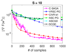
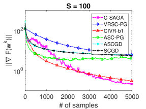
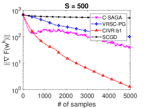
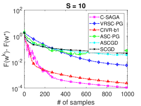
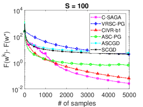
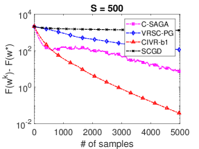
Figure 2: Experiments on policy evaluation for MDP for cases with $S=10$, $S=100$ and $S=500$.

Here we provide additional numerical experiments on the policy evaluation problem for MDP.

Let $\mathcal{S}=\{1,...,S\}$ be the state space of some Markov decision process. Suppose a reward of $R_{i,j}$ is received after transitioning from state $i$ to state $j$. Let $P^{\pi}\in\mathbf{R}^{S\times S}$ be the transition probability matrix under some fixed policy $\pi$. Then the evaluation of the value function $V^{\pi}:\mathcal{S}\to\mathbf{R}$ under such policy is equivalent to solving the following Bellman equation:

$$V^{\pi}(i)=\sum_{j=1}^{S}P^{\pi}_{i,j}(R_{i,j}+\gamma V^{\pi}(j))=\mathbf{E}_{j|i}[R_{i,j}+\gamma V^{\pi}(j)].$$

Following the suggestion of [6, 31], we apply the linear function approximation $V^{\pi}(i)\approx\langle\Psi_{i},w^{*}\rangle$ for a given set of feature vectors $\Psi_{i}$. and would like to compute the optimal vector $w^{*}$. This can be formulated as the following problem

$$\mathop{\textrm{minimize}}_{w}~{}F(w)\triangleq\sum_{i=1}^{S}\bigg{(}\langle\Psi_{i},w\rangle-\sum_{j=1}^{S}P^{\pi}_{i,j}(R_{i,j}+\gamma\langle\Psi_{j},w\rangle)\bigg{)}^{2}.$$

Let’s denote

$$q^{\pi}_{i}(w)\triangleq\sum_{j=1}^{S}P^{\pi}_{i,j}(R_{i,j}+\gamma\langle\Psi_{j},w\rangle)=\mathbf{E}_{j|i}[R_{i,j}+\gamma\langle\Psi_{j},w\rangle].$$

Then by defining

$$g(w)=\left[\langle\Psi_{1},w\rangle,...,\langle\Psi_{S},w\rangle,q^{\pi}_{i}(w),...,q^{\pi}_{S}(w)\right]^{T}$$

and

$$f(y_{1},...,y_{S},z_{1},...,z_{S})=\|y-z\|^{2}=\sum_{i=1}^{S}(y_{i}-z_{i})^{2},$$

the Least squares problem is transformed into the form of (2).

For this problem, we test the SCGD [30], the ASCGD [30], the ASC-PG [31], the VRSC-PG [12], C-SAGA [34] and our CIVR algorithms. In Section 5, we already tested the algorithms under their standard batch sizes, e.g. $\lceil n^{2/3}\rceil$ and $\lceil\sqrt{n}\rceil$. However, small constant batch sizes are often preferred in practice. Therefore, we would like to set the batch size to $s=1$ for all algorithms. For this special case, we denote the CIVR as the CIVR-b1. To balance the sample complexity between the initial full batch sampling and the later subsampling with $s=1$, we set the epoch length for VRSC-PG and CIVR-b1 to be $S$.

Note that the last $S$ components of $g$ are all independent expectations, therefore the variance reduction technique of VRSC-PG [12], C-SAGA [34] and CIVR-b1 applied to each of these components. In the experiments, $P^{\pi}$, $\Phi$ and $R^{\pi}$ are generated randomly.

Similar to the experiments performed in Section 5, the step sizes are chosen from $\{0.1,0.05,0.01,0.005,0.001,0.0005,0.0001\}$ by experiments for VRSC-PG, C-SAGA as well as for CIVR-b1. For $S=10$, $\eta=0.1$ works best for both C-SAGA and CIVR-b1, while $\eta=0.01$ works best for VRSC-PG; For $S=100$, $\eta=0.001$ works best for both C-SAGA and CIVR-b1, while $\eta=0.0001$ works best for VRSC-PG. For $S=500$, $\eta=0.0001$ works best for all three of them.

When $S=10$ and $S=100$, we choose $\alpha_{k}=0.01k^{-3/4}$ and $\beta_{k}=0.1k^{-1/2}$ for SCGD, $\alpha_{k}=0.01k^{-5/7}$ and $\beta_{k}=0.1k^{-4/7}$ for ASCGD and $\alpha_{k}=0.01k^{-1/2}$ and $\beta_{k}=0.1k^{-1}$ for ASC-PG. When $S=500$, we choose $\alpha_{k}=0.0001k^{-3/4}$ and $\beta_{k}=0.001k^{-1/2}$ for SCGD while ASCGD and ASC-PG fail to converge under various trials of parameters. The meaning of these step size parameters can be found in [31] and [30].

Figure 2 shows three experiments with sizes $S=10$, $S=100$ and $S=500$ respectively. We can see that both C-SAGA and CIVR-b1 preform much better than other algorithms in our setting. CIVR-b1 has more smooth and stable trajectory than C-SAGA.

References

Allen-Zhu [2017]
Zeyuan Allen-Zhu.
Natasha: Faster non-convex stochastic optimization via strongly
non-convex parameter.
In Proceedings of the 34th International Conference on Machine
Learning (ICML), volume 70 of Proceedings of Machine Learning
Research, pages 89–97, Sydney, Australia, 2017.
Allen-Zhu [2018]
Zeyuan Allen-Zhu.
Natasha 2: Faster non-convex optimization than SGD.
In Advances in Neural Information Processing Systems 31, pages
2675–2686. Curran Associates, Inc., 2018.
Allen-Zhu and Hazan [2016]
Zeyuan Allen-Zhu and Elad Hazan.
Variance reduction for faster non-convex optimization.
In Proceedings of the 33rd International Conference on Machine
Learning (ICML), pages 699–707, 2016.
Beck [2017]
Amir Beck.
First-Order Methods in Optimization.
MOS-SIAM Series on Optimization. SIAM, 2017.
Chaudhari et al. [2016]
Pratik Chaudhari, Anna Choromanska, Stefano Soatto, Yann LeCun, Carlo Baldassi,
Christian Borgs, Jennifer Chayes, Levent Sagun, and Riccardo Zecchina.
Entropy-sgd: Biasing gradient descent into wide valleys.
arXiv preprint, arXiv:1611.01838, 2016.
Dann et al. [2014]
Christoph Dann, Gerhard Neumann, and Jan Peters.
Policy evaluation with temporal differences: a survey and comparison.
Journal of Machine Learning Research, 15(1):809–883, 2014.
Defazio et al. [2014]
Aaron Defazio, Francis Bach, and Simon Lacoste-Julien.
SAGA: A fast incremental gradient method with support for
non-strongly convex composite objectives.
In Advances in Neural Information Processing Systems 27, pages
1646–1654, 2014.
Fang et al. [2018]
Cong Fang, Chris Junchi Li, Zhouchen Lin, and Tong Zhang.
Spider: Near-optimal non-convex optimization via stochastic
path-integrated differential estimator.
In Advances in Neural Information Processing Systems 31, pages
689–699. Curran Associates, Inc., 2018.
Ghadimi and Lan [2013]
Saeed Ghadimi and Guanghui Lan.
Stochastic first- and zeroth-order methods for nonconvex stochastic
programming.
SIAM Journal on Optimization, 23(4):2341–2368, 2013.
Gulcehre et al. [2016]
Caglar Gulcehre, Marcin Moczulski, Francesco Visin, and Yoshua Bengio.
Mollifying networks.
arXiv preprint, arXiv:1608.04980, 2016.
Hazan et al. [2016]
Elad Hazan, Kfir Yehuda Levy, and Shai Shalev-Shwartz.
On graduated optimization for stochastic non-convex problems.
In International conference on machine learning, pages
1833–1841, 2016.
Huo et al. [2018]
Zhouyuan Huo, Bin Gu, Ji Jiu, and Heng Huang.
Accelerated method for stochastic composition optimization with
nonsmooth regularization.
In Proceedings of the 32nd AAAI Conference on Artificial
Intelligence, pages 3287–3294, 2018.
Johnson and Zhang [2013]
Rie Johnson and Tong Zhang.
Accelerating stochastic gradient descent using predictive variance
reduction.
In Advances in Neural Information Processing Systems 26, pages
315–323, 2013.
Karimi et al. [2016]
Hamed Karimi, Julie Nutini, and Mark Schmidt.
Linear convergence of gradient method and proximal-gradient methods
under the Polyak-Łojasiewicz condition.
In Machine Learning and Knowledge Discovery in Database -
European Conference, Proceedings, pages 795–811, 2016.
Lei et al. [2017]
Lihua Lei, Cheng Ju, Jianbo Chen, and Michael I Jordan.
Non-convex finite-sum optimization via SCSG methods.
In Advances in Neural Information Processing Systems 30, pages
2348–2358. Curran Associates, Inc., 2017.
Li and Li [2018]
Zhize Li and Jian Li.
A simple proximal stochastic gradient method for nonsmooth nonconvex
optimization.
In Advances in Neural Information Processing Systems 31, pages
5564–5574. Curran Associates, Inc., 2018.
Lian et al. [2017]
Xiangru Lian, Mengdi Wang, and Ji Liu.
Finite-sum composition optimization via variance reduced gradient
descent.
In Proceedings of the 20th International Conference on
Artificial Intelligence and Statistics (AISTATS), pages 1159–1167, 2017.
Mobahi and Fisher [2015]
Hossein Mobahi and John W Fisher.
On the link between gaussian homotopy continuation and convex
envelopes.
In International Workshop on Energy Minimization Methods in
Computer Vision and Pattern Recognition, pages 43–56. Springer, 2015.
Nguyen et al. [2017]
Lam M. Nguyen, Jie Liu, Katya Scheinberg, and Martin Takáč.
SARAH: A novel method for machine learning problems using
stochastic recursive gradient.
In Doina Precup and Yee Whye Teh, editors, Proceedings of the
34th International Conference on Machine Learning (ICML), volume 70 of
Proceedings of Machine Learning Research (PMLR), pages 2613–2621,
Sydney, Australia, 2017.
Nguyen et al. [2019]
Lam M. Nguyen, Marten van Dijk, Dzung T. Phan, Phuong Ha Nguyen, Tsui-Wei Weng,
and Jayant R. Kalagnanam.
Finite-sum smooth optimization with sarah.
arXiv preprint, arXiv:1901.07648, 2019.
Pham et al. [2019]
Nhan H. Pham, Lam M. Nguyen, Dzung T. Phan, and Quoc Tran-Dinh.
ProxSARAH: An efficient algorithmic framework for stochastic
composite nonconvex optimization.
arXiv preprint, arXiv:1902.05679, 2019.
Reddi et al. [2016a]
Sashank J. Reddi, Ahmed Hefny, Suvrit Sra, Barnabas Poczos, and Alex Smola.
Stochastic variance reduction for nonconvex optimization.
In Proceedings of The 33rd International Conference on Machine
Learning, volume 48 of Proceedings of Machine Learning Research,
pages 314–323, New York, New York, USA, 2016a.
Reddi et al. [2016b]
Sashank J Reddi, Suvrit Sra, Barnabás Póczos, and Alex Smola.
Fast incremental method for smooth nonconvex optimization.
In 2016 IEEE 55th Conference on Decision and Control (CDC),
pages 1971–1977. IEEE, 2016b.
Reddi et al. [2016c]
Sashank J Reddi, Suvrit Sra, Barnabás Póczos, and Alexander J Smola.
Proximal stochastic methods for nonsmooth nonconvex finite-sum
optimization.
In Advances in Neural Information Processing Systems 29, pages
1145–1153, 2016c.
Rockafellar [1970]
R. Tyrrell Rockafellar.
Convex Analysis.
Princeton University Press, 1970.
Rockafellar [2007]
R. Tyrrell Rockafellar.
Coherent approaches to risk in optimization under uncertainty.
INFORMS TutORials in Operations Research, 2007.
Ruszczyński [2013]
Andrzej Ruszczyński.
Advances in risk-averse optimization.
INFORMS TutORials in Operation Research, 2013.
Sutton and Barto [1998]
Richard S Sutton and Andrew G Barto.
Reinforcement Learning: An Introduction.
MIT Press, Cambridge, MA, 1998.
Wang et al. [2017a]
Mengdi Wang, Ethan X Fang, and Han Liu.
Stochastic compositional gradient descent: algorithms for minimizing
compositions of expected-value functions.
Mathematical Programming, 161(1-2):419–449, 2017a.
Wang et al. [2017b]
Mengdi Wang, Ji Liu, and Ethan Fang.
Accelerating stochastic composition optimization.
Journal of Machine Learning Research, 18(105):1–23, 2017b.
Wang et al. [2018]
Zhe Wang, Kaiyi Ji, Yi Zhou, Yingbin Liang, and Vahid Tarokh.
SpiderBoost: A class of faster variance-reduced algorithms for
nonconvex optimization.
arXiv preprint, arXiv:1810.10690, 2018.
Xiao and Zhang [2014]
Lin Xiao and Tong Zhang.
A proximal stochastic gradient method with progressive variance
reduction.
SIAM Journal on Optimization, 24(4):2057–2075, 2014.
Zhang and Xiao [2019]
Junyu Zhang and Lin Xiao.
A composite randomized incremental gradient method.
In Proceedings of the 36th International Conference on Machine
Learning (ICML), number 97 in Proceedings of Machine Learning Research
(PMLR), Long Beach, California, 2019.
Zhou et al. [2018]
Dongruo Zhou, Pan Xu, and Quanquan Gu.
Stochastic nested variance reduced gradient descent for nonconvex
optimization.
In Advances in Neural Information Processing Systems 31, pages
3921–3932. Curran Associates, Inc., 2018.