The Power of Unbiased Recursive Partitioning:
A Unifying View of CTree, MOB, and GUIDE

The Power of Unbiased Recursive Partitioning Lisa Schlosser, Torsten Hothorn, Achim Zeileis A core step of every algorithm for learning regression trees is the selection of the best splitting variable from the available covariates and the corresponding split point. Early tree algorithms (e.g., AID, CART) employed greedy search strategies, directly comparing all possible split points in all available covariates. However, subsequent research showed that this is biased towards selecting covariates with more potential split points. Therefore, unbiased recursive partitioning algorithms have been suggested (e.g., QUEST, GUIDE, CTree, MOB) that first select the covariate based on statistical inference using $p$-values that are adjusted for the possible split points. In a second step a split point optimizing some objective function is selected in the chosen split variable. However, different unbiased tree algorithms obtain these $p$-values from different inference frameworks and their relative advantages or disadvantages are not well understood, yet. Therefore, three different popular approaches are considered here: classical categorical association tests (as in GUIDE), conditional inference (as in CTree), and parameter instability tests (as in MOB). First, these are embedded into a common inference framework encompassing parametric model trees, in particular linear model trees. Second, it is assessed how different building blocks from this common framework affect the power of the algorithms to select the appropriate covariates for splitting: observation-wise goodness-of-fit measure (residuals vs. model scores), dichotomization of residuals/scores at zero, and binning of possible split variables. This shows that specifically the goodness-of-fit measure is crucial for the power of the procedures, with model scores without dichotomization performing much better in many scenarios. classification and regression trees, independence tests, recursive partitioning, simulation Lisa Schlosser, Achim Zeileis
Universität Innsbruck
Department of Statistics
Faculty of Economics and Statistics
Universitätsstr. 15
6020 Innsbruck, Austria
E-mail: ,
URL: https://www.uibk.ac.at/statistics/personal/schlosser-lisa/,
URL: https://eeecon.uibk.ac.at/~zeileis/
Torsten Hothorn
Universität Zürich
Institut für Epidemiologie, Biostatistik und Prävention
Hirschengraben 84
8001 Zürich, Switzerland
E-mail:
URL: http://user.math.uzh.ch/hothorn/

1 Introduction

In many situations fitting one global model to a given data set can be very challenging, especially if the data contains lots of different features with strong variation and complex interactions. Therefore, separating the data into more homogeneous subgroups based on a set of covariates first can simplify the task and fitting a local model to each of the resulting subgroups often leads to better results. This separation can be done by applying a tree algorithm. While almost all algorithms proposed in the literature follow the general idea of splitting the data such that some objective function is optimized locally, they differ in their specific approaches to selecting a split variable and the corresponding split point. Some of the first tree algorithms (e.g., AID, Morgan and Sonquist, 1963; CART, Breiman et al., 1984) rely on exhaustive search procedures to find both, the best split point and split variable in one step by directly comparing all possible split points in all possible split variables. However, it has been shown that this is not only computationally expensive but also biased towards split variables with many possible split points (Doyle, 1973; Kim and Loh, 2001). Therefore, selecting a split variable in a first step and then searching for the best split point only within this variable in a separated second step is a more promising strategy as applied for example by the algorithms QUEST (Loh and Shih, 1997), GUIDE (Loh, 2002), CTree (Hothorn et al., 2006b) and MOB (Zeileis et al., 2008). For the first step of selecting a split variable they all share the same basic concept of choosing the covariate which shows the highest association to the response variable based on $p$-values provided by a statistical test. While QUEST and GUIDE employ statistical significance tests for contingency tables, CTree applies permutation tests in a conditional inference framework and MOB uses fluctuation tests based on central limit theorems for the parameter estimators. All these approaches have been shown to work well for various situations, however, the relative (dis)advantages of the testing strategies have not yet been investigated and compared in detail.

Therefore, in this paper the focus will be put on that first step of tree algorithms, i.e., the task of selecting the best split variable in a given (sub)sample. In particular, the approach of the GUIDE algorithm is compared to the one of the CTree algorithm and the MOB algorithm by investigating the building blocks of their testing strategies in which they differ: (1) Variation of the goodness-of-fit measure for the response: using residuals or full model scores. (2) Dichotomization of these residuals or scores. (3) Categorization of possible split variables. Apart from these three main factors further aspects such as the approximation of the null distribution (conditional vs. unconditional) or the type of test statistic (maximally selected vs. sum of squares) will be considered as well. For this purpose, a unifying framework for testing strategies in unbiased model-based tree algorithms is presented such that each of the three strategies in GUIDE, CTree, and MOB can be obtained by a specific combination of the available building blocks. This allows to systematically vary the building blocks and assess the power of the resulting inference procedure. Moreover, it is investigated whether the performance of the inference impacts the performance of the trees differently under pre- vs. post-pruning.

In many of the considered scenarios the choice of goodness-of-fit measure heavily influences the performance of testing strategies. In particular, using model scores leads to overall clearly better results than employing residuals only. Moreover, the original values of the goodness-of-fit measure are preferred over dichotomized versions of them. Also regarding the effects of categorizing possible split variables and the selection of a pruning strategy clear recommendations can be given based on the presented results.

The remainder of this manuscript is structured as follows: Section 2 reviews unbiased tree models, starting with the general algorithmic idea (Section 2.1) followed by the specific algorithms CTree (Section 2.2), MOB (2.3), and GUIDE (2.4), before possible pruning strategies (2.5) are discussed. In Section 3 the unifying framework for testing strategies in unbiased model-based recursive partitioning algorithms is presented. The setting for the simulation study is introduced in Section 4 and the results are illustrated and discussed in Section 5.

2 Unbiased recursive partitioning

2.1 Generic algorithm

The basic idea of building a regression tree model is to partition the data into smaller and more homogeneous subgroups based on a set of covariates. Various tree algorithms have been developed, following essentially the same general structure, employing the covariates as split variables in the tree induction. Starting at the root of the tree, pertaining to the full available data sample, the algorithms proceed in the following steps:

1. For the current sample a (possibly simple) model is fitted by optimizing some objective function (or loss function) that reflects the goodness of fit.

2. Among all available split variables one is selected as the split variable, choosing the split point such that goodness of fit is maximized in the resulting subgroups.

3. Steps 1 and 2 are repeated within each subgroup until some stopping criterion is attained.

The term “model” is used here in a very broad sense and encompasses not only least-squares or maximum-likelihood models but also simple constant fits such as means or average proportions. Therefore, depending on the type of model, the employed objective function can for example be the sum of deviations from a typical/average value, but it can also be based on a model for a response along with potential split variables. For instance, different types of residuals (or the signs thereof) can be employed (see e.g., Loh, 2002) as well as rank sums or logrank scores (as in Hothorn et al., 2006a).

As explained in Section 1 the considered tree algorithms CTree, MOB, and GUIDE first select the split variable and then, in a separate step, the split point. For the first step of selecting a split variable they all apply statistical tests following the same basic strategy:

1. To capture how the objective function changes with the observations in the current subgroup, a disaggregated, observation-wise goodness-of-fit measure is obtained. More formally, this is an $N\times K$ matrix where $N\in\mathbb{N}$ is the number of observations and $K\in\mathbb{N}$ the number of goodness-of-fit measures per observation.

2. The dependency or association of this goodness-of-fit matrix with each possible split variable $Z_{j}$, $j\in\{1,\dots,J\}$, is assessed using some suitable test statistic. The corresponding $p$-values allow for a comparison of all $J$ split variables on a standardized or unified scale and in that way for an unbiased split variable selection.

3. The split variable corresponding to the smallest $p$-value – and thus the highest influence on the goodness of fit of the model – is selected for splitting the data into subgroups.

As an example – and explained in more detail below – consider a linear regression tree. Thus, a linear regression model is fitted in each subgroup, minimizing the residual sum of squares as the aggregated goodness-of-fit measure. The corresponding observation-wise goodness-of-fit measure can be given by the residuals or the scores (gradient contributions). Analogously, the log-likelihood and corresponding score function could be used.

While this basic approach is the same for the GUIDE, CTree, and MOB algorithms, they differ in their strategies on how to calculate test statistics. In order to point out these specific characteristics in Section 3 the strategies of the three tree algorithms are first explained in more detail in Sections 2.2, 2.3, and 2.4.

2.2 CTree

The CTree algorithm (Hothorn et al., 2006b) is based on the idea of providing non-parametric regression tree models in a conditional inference framework by applying permutation tests. To select a split variable it is tested whether there is any association between the transformed response $h(Y)$ and each possible transformed split variable $g(Z_{j})$, $j=1,\dots,J$. The only requirement for the function $h$ is to depend on $Y$ in a permutation-symmetric way but this encompasses ranks, scores, indicator functions, etc. and can also be multidimensional. For a numeric response the identity function $h(Y)=Y$ is a common choice while a categorical response can be mapped to a unity vector by an indicator function $h(Y)=(0,\ldots,1,\ldots,0)^{\top}$. Alternatively, the function $h$ can capture location and scale of $Y$ via $h(Y)=(Y,(Y-\bar{Y})^{2})^{\top}$. If a parametric model is fitted to the response $Y$ with some covariate(s) $X$ employed as regressor variable(s), then a model-based transformation $h(Y)=s(Y,X,\hat{\beta})$ can be used, e.g., the residuals in a linear model with regression coefficients $\beta$. Moreover, $s$ can be the score function pertaining to the objective function (or loss function) $\ell$:

$$s(Y,X,\beta)=\frac{\partial\ell(Y,X,\beta)}{\partial\beta}$$

The estimate of the model parameters $\hat{\beta}$ is obtained by optimizing the sum of the objective function $\ell$, aggregated over all observations. This framework includes many different M-type estimators as special cases, including maximum likelihood and ordinary least squares estimation. For a $K$-dimensional parameter $\beta$ the score function evaluated for the $i$-th observation $s(y_{i},x_{i},\beta)$ is also a $K$-dimensional vector, i.e., the gradient contribution of the $i$-th observation. Thus, the $N\times K$-matrix consisting of these scores or gradient contributions for all $i=1,\dots,N$ observations is a natural candidate for the observation-wise goodness-of-fit measure as described in the previous Section 2.1.

Similarly, different types of functions can be chosen for the influence function $g$ depending on a possible split variable $Z$. A simple choice in case of $Z$ being a numeric variable is again the identity function $g(Z)=Z$. For categorical variables $g$ can also map its values to the corresponding unity vectors by an indicator function $g(Z)=(0,\ldots,1,\ldots,0)^{\top}$.

To test for independence of $h(Y)$ and $g(Z)$ CTree calculates a linear association test statistic, following the framework of Strasser and Weber (1999). The corresponding conditional expectation and covariance given all permutations of the response variable can be calculated and used to standardize the test statistic. This standardized statistic has an asymptotic normal distribution which is in fact multivariate if either of the transformation $h(Y)$ and/or $g(Z)$ is multivariate. The actual test is carried out by mapping this standardized statistic to the real line either by taking the absolute maximum or using a quadratic form – with $p$-values being computed from the analogous transformation of the normal distribution (see Hothorn et al., 2006a, for a hands-on introduction and Appendix A.1 for more details on the linear test statistic).

If both variables $Y$ and $Z$ are numeric the default independence test corresponds to a Pearson correlation test. For one numeric and one categorical variable essentially a one-way ANOVA (analysis of variance) is employed while for two categorical variables a $\chi^{2}$ test is performed. Thus, in the general CTree framework many types of tests can be specified by selecting suitable transformations $g$ and $h$. While originally conceived for nonparametric models, it is easy to adapt CTree to model-based testing and recursive partitioning by choosing a model-based $h$ transformation as argued above (see the concrete examples in Zeileis and Hothorn, 2013; Seibold et al., 2016).

2.3 MOB

In contrast to CTree the MOB algorithm (Zeileis et al., 2008) was explicitly designed for a model-based goodness-of-fit measure in order to embed parametric models into a regression tree framework. Thus, MOB is based on an objective/loss function $\ell$ and corresponding score function $s$. The original paper considered generalized linear models (GLMs) and survival regression models but subsequently various other models have been applied as well, including beta regression (Grün et al., 2012), psychometric item response theory models (Strobl et al., 2015), or mixed effects models (Fokkema et al., 2018). But just like CTree can be applied to parametric models, MOB conversely also encompasses simple regression and classification trees, e.g., by choosing an intercept-only model.

For selecting a split variable MOB employs a score-based test that relies on the central limit theorem for the parameter estimate $\hat{\beta}$. The test assesses whether the scores – when ordered by the potential split variable $Z$ – fluctuate randomly around their zero mean or differ systematically in certain subgroups. The latter would indicate a parameter instability that could be captured by fitting separate models (optimizing $\ell$) in the resulting subgroups. In case of a numeric split variable $Z$ both the score-based statistic and the partitioned objective function $\ell$ are maximized over all possible splits in $Z$ (subject to certain minimal subgroup size constraints). Unlike the CTree framework, MOB relies on classical unconditional inference. For more details see Zeileis and Hornik (2007) and Appendix A.2.

2.4 GUIDE

Building on earlier work for the QUEST algorithm (Loh and Shih, 1997), Loh (2002) proposed the GUIDE algorithm blending trees with parametric regression models and encompassing simpler classification and regression trees as special cases. Thus, linear regression models could be fitted in the nodes of a tree as well as constant fits such as simple mean response $\hat{\beta}=\bar{y}=\frac{1}{N}\sum_{i=1}^{N}y_{i}$. The tests for selecting the split variable are then based on the corresponding residuals, e.g., for a simple linear regression (as used in Loh, 2002):

$$r(Y,X,\hat{\beta})=Y-\hat{\beta_{0}}-\hat{\beta_{1}}\cdot X.$$

In subsequent work other models together with an appropriate choice of residuals have been applied such as in regression trees for longitudinal and multiresponse data (Loh and Zheng, 2013), quantile regression models (Chaudhuri and Loh, 2002), and proportional hazards modeling via Poisson regression (Loh et al., 2015), among others.

To construct a statistical test two additional transformations are carried out: (1) The residuals $r(Y,X,\hat{\beta})$ are dichotomized at zero, yielding an indicator for positive vs. negative residuals. (2) Each possible split variable $Z$ is categorized, i.e., unless $Z$ is already categorical it is split at its quartiles into four bins. Subsequently, a $\chi^{2}$ test of independence is performed for the dichotomized residuals and each categorized/categorical split variable. After choosing the split variable showing the highest dependency by yielding the lowest $p$-value, the split point minimizing the overall goodness-of-fit measure is selected. Note that the split point in numeric variables $Z$ is searched over all possible splits, not just the four bins that were constructed for the $\chi^{2}$ test. More details on the applied test statistic can be found in Appendix A.3.

2.5 Pruning

To avoid overfitting recursive partitioning algorithms need to assure that trees do not grow too large. Apart from certain minimal subgroup size or maximal tree depth constraints this is classically accomplished by so-called “pruning” approaches. As the three tree algorithms considered here (CTree, MOB, and GUIDE) differ in their default choice of pruning approach, we briefly discuss these here. However, as all three algorithms can in principle be combined with any of the pruning approaches this is done only relatively briefly.

The classical CART algorithm (Breiman et al., 1984) proposed to first grow a large tree and then prune those splits in the tree that did not increase predictive performance in a cross-validation. This is also know as post-pruning (after growing the initial tree) and more specifically cost-complexity pruning.

In the unbiased recursive partitioning literature this post-pruning approach is also used frequently (e.g., in Loh and Vanichsetakul, 1988; Loh and Shih, 1997; Kim and Loh, 2001; Loh, 2002) and the $p$-values from the association tests are only employed for selecting the split variable on a unified scale. However, Hothorn et al. (2006b) proposed to also use these $p$-values for a so-called pre-pruning strategy which stops growing the tree as soon as no significant association can be found in a given subgroup. This approach is the default in CTree and also in MOB. However, Zeileis et al. (2008) also pointed out that a natural strategy for post-pruning in model-based partitioning is to use information criteria such as AIC (Akaike information criterion) or BIC (Bayes information criterion), following the ideas of Su et al. (2004).

Clearly, for inference-based pre-pruning it is crucial that the association tests employed for split selection work well as statistical significance test, i.e., conform with their nominal size and have high power. In contrast, when using post-pruning (either based on cross-validation or information criteria) it might not be as crucial that the significance test works well and has high power.

Due to these considerations we first evaluate the significance tests underlying CTree, MOB, and GUIDE by themselves, i.e., without growing an actual tree in combination with a pruning strategy. Subsequently we combine the tests with a cost-complexity post-pruning approach in order to assess whether shortcomings of the tests are mitigated by pruning.

3 Unifying framework

Each of the algorithms CTree, GUIDE, and MOB can be characterized by its combination of the type of model fits, tests, and pruning strategy employed to grow the tree. Table 1 provides an overview of the default combinations. However, as discussed above, subsequent publications have emphasized that all three algorithms can be combined with different model fitting approaches and to some degree different pruning strategies have been explored as well. Thus, the class of tests employed for the unbiased splitting variable selection forms the core of each of the algorithms: conditional inference (CTree) vs. score-based fluctuation tests (MOB) vs. residual-based $\chi^{2}$ tests (GUIDE). Therefore, we consider a standard class of model fits (namely, linear regression trees) and investigate the relative advantages and disadvantages of the tests themselves (which are essential to pre-pruning) as well as the combination with post-pruning. Thus, subsequently the names CTree, MOB, and GUIDE distinguish the test-based variable and split selection rather than the entire algorithm with all default settings.

	Fit	Test	Pruning
CTree	Non-parametric	Conditional inference	Pre
MOB	Parametric	Score-based fluctuation	Pre (or post with AIC/BIC)
GUIDE	Parametric	Residual-based $\chi^{2}$	Post (cost-complexity pruning)

Table 1: Default combinations of fitted model type, test type and pruning strategy for the algorithms CTree, MOB, and GUIDE.

3.1 Building blocks of testing strategies

Even though CTree, MOB, and GUIDE differ in the specific tests they apply, their approaches for split variable selection follow the same basic structure as explained in Section 2.1. In fact, the tests can be embedded in a unifying conceptual framework that yields the different tests by combining various building blocks. These mostly differ in the way the model for the dependent variable on the one hand and the splitting variables on the other are prepared or transformed:

• Goodness-of-fit measure:
  Different variations of the disaggregated, observation-wise goodness-of-fit measure of the model for the response $Y$ and possible regressors $X$ can be considered. Either residuals $r(Y,X,\hat{\beta})$ can be used as proposed for GUIDE or model scores $s(Y,X,\hat{\beta})$ as proposed for MOB. All three algorithms can, in principle, use both goodness-of-fit measures though, which is probably brought out most clearly in the CTree algorithm that explicitly allowed for different transformations $h(Y)$ in its original description already.

• Dichotomization of residuals/scores:
  Rather than testing independence between the split variables and the residuals/scores themselves, it is possible to dichotomize residuals/scores at $0$ so that only their signs are assessed (as proposed for GUIDE).

• Categorization of split variables:
  Similarly, the split variables can also be categorized (for testing only). This was proposed for GUIDE, employing binning at the quartiles yielding four categories of approximately equal size.

The three algorithms combine these building blocks in different ways as shown in Table 2: When applying CTree for unbiased model-based recursive partitioning it has been suggested to use the model scores without dichotomization and assess their association with the untransformed split variables using a conditional inference test. This is similar to a squared correlation test statistic. MOB also employs the scores without dichotomization and maximally selects a score statistic over all potential split points in the split variable. GUIDE employs the dichotomized residuals and assesses their association with the categorized split variable in a classical (unconditional) $\chi^{2}$ test.

But the building blocks could be easily re-combined to yield new types of tests. For example, in the GUIDE approach, a one-way ANOVA can be used for assessing the association of the residuals (without dichotomization) with the categorized split variable. Or alternatively, a multivariate one-way ANOVA can be used for the non-dichotomized scores as opposed to the residuals etc.

Note that there are further differences in the testing strategies between the three algorithms, e.g., using conditional vs. unconditional approximations of the null distributions. However, this difference has relatively little influence compared to the other building blocks considered in detail here. Moreover, both similarities and relative differences between these approaches have been previously discussed, e.g., in Hothorn and Zeileis (2008) and Zeileis and Hothorn (2013).

	Scores	Dich.	Cat.	Statistic
CTree	Model scores	–	–	Sum of squares
MOB	Model scores	–	–	Maximally selected
GUIDE	Residuals	✓	✓	Sum of squares

Table 2: Testing strategies of CTree, MOB, and GUIDE with the corresponding setting of the building blocks in the unifying framework and the type of test statistic.

3.2 Linear model tree

To focus on the unified testing framework, as described in the previous section, we employ the same model fits for all three algorithms. To do so, we employ linear regression models because it is such a basic and widely used model and linear model trees were the leading illustrations in both the original MOB (Zeileis et al., 2008) and GUIDE (Loh, 2002) papers. However, the conclusions drawn from this example also hold for many other model types.

To fix notation, we consider the following models for the simulation study in Section 4:

$$Y=\beta_{0}+\beta_{1}\cdot X+\epsilon$$

with response variable $Y$, regressor variable $X$, and error term $\epsilon$. In particular, in the investigated tree models the coefficients $\beta_{0}$ and $\beta_{1}$ can depend on the possible split variables $Z_{j}$, $j=1,\ldots,J$, such that

$$Y=\beta_{0}(Z_{1},\ldots,Z_{J})+\beta_{1}(Z_{1},\ldots,Z_{J})\cdot X+\epsilon.$$

This model is fitted, as usual, by ordinary least squares (OLS) to the observations in each notation, yielding the parameter estimates $\hat{\beta}=(\hat{\beta_{0}},\hat{\beta_{1}})^{\top}$. To keep notation simple we present the following equations for the root node with all observations $\{(y_{i},x_{i})\}_{i=1,\ldots,N}$ and $N\in\mathbb{N}$. In subsequent nodes the same equations are used but just for a smaller subgroup.

The aggregated goodness-of-fit measure (or objective or loss function) in OLS estimation is the sum of squared residuals: $\sum_{i=1}^{N}\ell(y_{i},x_{i},\beta_{0},\beta_{1})$ where

$$\ell(y_{i},x_{i},\beta_{0},\beta_{1})=r(y_{i},x_{i},\beta_{0},\beta_{1})^{2}$$

is the squared residual which is defined as

$$r(y_{i},x_{i},\beta_{0},\beta_{1})=y_{i}-\beta_{0}-\beta_{1}\cdot x_{i}.$$

These residuals can also intuitively be used as the corresponding disaggregated observation-wise goodness-of-fit measure. Another natural candidate for this is the score function for the $i$-th observation:

$$s(y_{i},x_{i},\beta_{0},\beta_{1})=\frac{\partial\ell}{\partial(\beta_{0},\beta_{1})^{\top}}(y_{i},x_{i},\beta_{0},\beta_{1})=-2\cdot r(y_{i},x_{i},\beta_{0},\beta_{1})\cdot(1,x_{i})^{\top}$$

Thus, up to a constant scaling factor of $-2$ (that could also be omitted) the first component of the scores is in fact the residual. However, it is complemented by a second component that captures the slope effect of $x_{i}$. Therefore, when computing the score for all $N$ observations this yields an $N\times 2$ score matrix whose first column corresponds to the $N$ residuals. As this is the derivative with respect to the intercept parameter $\beta_{0}$, it captures changes in the intercept. Moreover, the second column of the score matrix contains derivatives with respect to the slope parameter $\beta_{1}$ and thus captures changes in this.

Hence, tests based on the full scores (as in CTree and MOB) include residual-based tests (as in GUIDE) as a special case. Therefore, score-based tests can in principle capture all changes in the objective function that residual-based tests can capture – but the reverse is not necessarily true. In the next sections we will investigate how relevant this is in practice and how much it depends on the concrete test statistics employed.

4 Simulation setting and evaluation

In this simulation study two different scenarios are considered for the linear model trees presented in Section 3.2. First, the underlying tree structure based on which the data is generated is a stump, i.e., a tree with only one split (“stump” scenario, see Figure 1). By keeping the tree so simple we can focus on the testing strategy only giving focus to their power in terms of selecting the correct split variable.

In the second scenario the true tree structure contains two splits in two different variables yielding a tree with three terminal nodes (“tree” scenario, see Figure 2). It employs the same basic structure as the first scenario but simply adds another split. This allows to evaluate the power of the three testing strategies in a more complex setting, in combination with using a post-pruning strategy.

4.1 Data generating process

4.1.1 “Stump” scenario

Each generated data set consists of the response and regressor variables, one true split variable and nine noise split variables as listed in Table 3 together with the corresponding distributions.

Name	Notation	Specification
Variables:
Response	$Y$	$=\beta_{0}(Z_{1})+\beta_{1}(Z_{1})\cdot X+\epsilon$
Regressor	$X$	$\mathcal{U}([-1,1])$
Error	$\epsilon$	$\mathcal{N}(0,1)$
True split variable	$Z_{1}$	$\mathcal{U}([-1,1])$
Noise split variables	$Z_{2}$–$Z_{10}$	$\mathcal{U}([-1,1])$ or $\mathcal{N}(0,1)$
		(alternating)
Parameters/functions:
Intercept	$\beta_{0}$	$0$ or $\pm\delta$
Slope	$\beta_{1}$	$1$ or $\pm\delta$
True split point	$\xi$	$\in\{0,0.2,0.5,0.8\}$
Effect size	$\delta$	$\in\{0,0.1,0.2,\ldots,1\}$

Table 3: Variables included in the data generating process as used for the “stump” scenario. In the “tree” scenario $Z_{2}$ is also a true split variable, not only $Z_{1}$, and hence $\beta_{0}$ and $\beta_{1}$ are functions $\beta_{k-1}(Z_{1},Z_{2})$, $k=1,2=K$.

The location parameter $\mu$ of the normally distributed response variable $Y$ depends linearly on the regressor variable $X$. Moreover, the intercept $\beta_{0}$ and/or the slope parameter $\beta_{1}$ can depend on the true split variable $Z_{1}$. More specifically, three different variations are considered for the coefficients $\beta_{0}$ and $\beta_{1}$:

1. The intercept $\beta_{0}$ varies depending on $Z_{1}$ while $\beta_{1}$ is fixed (at $1$).

2. The slope coefficient $\beta_{1}$ varies depending on $Z_{1}$ while $\beta_{0}$ is fixed (at $0$).

3. Both coefficients $\beta_{0}$ and $\beta_{1}$ vary depending on $Z_{1}$.

See Figure 1 for an illustration. More precisely, the coefficient that changes ($\beta_{k-1}$ with $k=1,2=K$) switches between two values at the split point $\xi$:

$$\beta_{k-1}(Z_{1})=\begin{cases}-\delta\cdot(-1)^{k-1}\quad\text{if }Z_{1}\leq\xi\\ +\delta\cdot(-1)^{k-1}\quad\text{if }Z_{1}>\xi\end{cases}$$

In that way, the type of variation is the same for $\beta_{0}$ and $\beta_{1}$, however, in opposite directions.

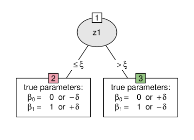
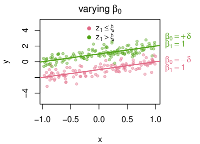
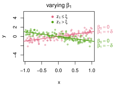
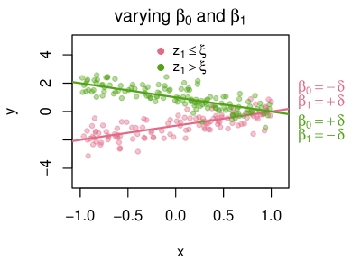
Figure 1: Top left panel: True stump structure applied in the data generating process for the “stump” scenario with the true model parameters $\beta_{0}$ and $\beta_{1}$, either varying or being fixed at $0$ or $1$ respectively. Top right and bottom panels: Bivariate plot of the response $Y$ on regressor $X$ with effect size $\delta=1$ and for three variations: varying $\beta_{0}$ and fixed $\beta_{1}$ (top right), fixed $\beta_{0}$ and varying $\beta_{1}$ (bottom left), varying $\beta_{0}$ and varying $\beta_{1}$ (bottom right).

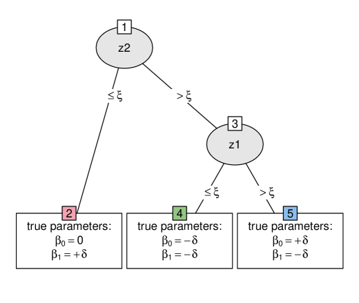
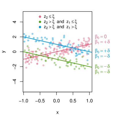
Figure 2: Left panel: True tree structure applied in the data generating process for the “tree” scenario with the true model parameters $\beta_{0}$ and $\beta_{1}$ for each terminal panel. Right panel: Bivariate plot of the response $Y$ on regressor $X$ with effect size $\delta=1$.

4.1.2 “Tree” scenario

For the second simulation scenario (“tree” scenario, see Figure 2) the same basic setting with the same variables as in the “stump” scenario is applied (see Table 3). However, not only $Z_{1}$ but also $Z_{2}$ is used as a true split variable following a uniform distribution on $[-1,1]$. Therefore, an additional split is preformed yielding a tree with three terminal nodes. The first split (in $Z_{2}$, at $\xi$) induces a change in the slope parameter $\beta_{1}$ while the second split (in $Z_{1}$, also at $\xi$) corresponds to a change in the intercept $\beta_{0}$. Hence, contrary to the “stump” scenario where three variations are considered for the parameters $\beta_{0}$ and $\beta_{1}$, only this one variation with both parameters varying is investigated for the “tree” scenario. In particular, the parameters depend on the split variables in the following way:

$$\beta_{0}(Z_{1},Z_{2})=\begin{cases}0\qquad\text{if }Z_{2}\leq\xi\\ -\delta\quad\text{ if }Z_{1}\leq\xi\land Z_{2}>\xi\\ +\delta\quad\text{ if }Z_{1}>\xi\land Z_{2}>\xi\end{cases}$$

$$\beta_{1}(Z_{1},Z_{2})=\beta_{1}(Z_{2})=\begin{cases}+\delta\quad\text{if }Z_{2}\leq\xi\\ -\delta\quad\text{if }Z_{2}>\xi\end{cases}$$

4.2 Evaluation

The testing strategies are evaluated over a stepwise increasing effect size $\delta$, on 100 replications per step each consisting of 250 observations. To compare the performance of the evaluated testing strategies for each step in the “stump” scenario the following criteria are considered: the $p$-values pertaining only to the true split variable $Z_{1}$; and the proportion of replications for which the $p$-value of $Z_{1}$ is the lowest and significant at 5% level (i.e., where $Z_{1}$ would be selected for splitting in a pre-pruning approach), denoted by the “selection probability”. In that way, the power of the considered statistical tests can be compared as they are all applied as significance tests answering two questions at once: (1) Should a split be performed at all? (2) If so, in which variable? For the first question the $p$-values regarding all available split variables are compared to a predefined level of significance $\alpha=0.05$. Only if the smallest $p$-value is smaller than $\alpha$ a split is performed and the split variable corresponding to this $p$-value is selected.

For the “tree” scenario the adjusted Rand index (ARI) is calculated as a measure of similarity between the true tree structure and the fitted model tree.

As explained before, the aim of this simulation study is to investigate the effects of each particular building block of the unifying framework presented in Section 3 rather than the whole testing strategies. Therefore, other combinations as presented in Table 2, hence adapted versions of GUIDE, CTREE, and MOB are evaluated as well as their original versions.

5 Results

In the following we first investigate the properties of the testing strategies in the “stump” scenario, focusing on the tests’ $p$-values for the true split variable $Z_{1}$ and its corresponding selection probability (i.e., the association of $Y$ and $Z_{1}$ being significant at 5% level and having the lowest $p$-value among all split variables). Section 5.1 begins by highlighting the importance of using full model scores vs. residuals only before Section 5.2 considers all building blocks (scores vs. residuals, dichotomization of these, and categorization of the split variable). Subsequently, the “tree” scenario is employed to investigate how the performance of the tests affects growing the trees overall. This is evaluated using the adjusted Rand index for trees grown by pre-pruning and cost-complexity post-pruning (Section 5.3).

5.1 “Stump” scenario: Residuals vs. full model scores

A crucial difference between the testing strategies of CTree/MOB and GUIDE is the difference between using only the residuals vs. the full model scores. In the literature on structural change tests it is well-established that residual-based tests can only capture parameter differences that affect the conditional mean (see e.g., Ploberger and Krämer, 1992, and further discussion in Section 6). Hence we compare the CTree, MOB, and GUIDE algorithms – all three using the default specification as shown in Table 2 – and additionally consider a new GUIDE flavor, denoted GUIDE+scores, that uses dichotomized scores rather than residuals.

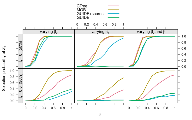
Figure 3: Selection probability of the true split variable $Z_{1}$ for testing strategies CTree, MOB, GUIDE, and GUIDE+scores in the “stump” scenario. Probabilities are estimated over increasing effect size $\delta$ with 100 replications of 250 observations per step. The true split point in $Z_{1}$ is either the median 0 (top) or the 90% quantile 0.8 (bottom) for either varying intercept $\beta_{0}$ (left), varying slope $\beta_{1}$ (middle), or both coefficients varying (right).

In Figure 3 the performances of the testing strategies are represented by the corresponding selection probability, i.e., a significance level is incorporated. (Appendix C shows that the same qualitative conclusions can be drawn when the significance level is not included.) For a split point at the median ($\xi=0$, top row) all testing strategies perform similarly well as long as the intercept varies (left and right panel) with CTree and MOB being only slightly ahead. However, for the split point at the $90$% quantile $\xi=0.8$ (bottom row) the performance of all of the applied strategies decreases. While both GUIDE versions struggle to detect the correct split variable even for a high effect size, MOB is clearly ahead with CTree leading to the second best results. This advantage of MOB over CTree is mainly due to the abrupt shift in the model parameters $\beta_{0}$ and $\beta_{1}$ and turns into an advantage of CTree over MOB for a smooth transition with continuously-changing parameters (see Appendix D).

However, in the scenario where only $\beta_{1}$ (but not the intercept $\beta_{0}$) is affected by the split, the residual-based GUIDE approach has no power at all even for a true split at the median (top middle panel). It is easily possible, though, to substantially mitigate this problem by using scores (sensitive to changes in all parameters) rather than residuals only (sensitive to changes in the conditional mean). The remaining difference between MOB/CTree and GUIDE+scores is due to dichotomizing the scores at zero and due to categorizing the split variables which are investigated in more detail in the following section.

5.2 “Stump” scenario: Full factorial analysis of building blocks

To investigate the impact of each of the building blocks separately the most general case of the “stump” scenario where the intercept and slope parameter are both varying is considered. In this evaluation all possible combinations of the building blocks have been included. The different levels of each of the three building blocks are listed in Table 4 where $h$ and $g$ refer to the transformation functions applied to the response $Y$ or a split variable $Z$ respectively, both as described in Section 2.2.

In the case of categorization, the split variable $Z$ is binned at the quartiles. This corresponds to a four-dimensional 0/1 transformation function $g(Z)$ that indicates into which of the bins each observation falls. Maximum selection across potential split points in a variable $Z$ also corresponds to a multivariate 0/1 transformation function $g(Z)$. However, in this case for each potential split point an indicator is used that is 0 before and 1 after the respective split point. (See also Table 5 in Appendix B for a more detailed overview of all 12 combinations of the building blocks.)

Building block	Levels	Transformation
Residuals vs. scores	residuals	$h(Y)=r(Y,X,\hat{\beta})$
($h$ transformation)	scores	$h(Y)=s(Y,X,\hat{\beta})$
Dichotomization	yes	$\mathds{1}_{[0,\infty)}(h)$
(of $h$)	no	$h$ without
		dichotomization
Categorization	cat	$g(Z)=(0,1,0,0)^{\top}$
($g$ transformation)		indicating the
		assigned bin
	max	$g(Z)=(0,\ldots,0,1,\ldots,1)^{\top}$
		indicating the
		potential split point
	lin	$g(Z)=Z$

Table 4: Available levels of the building blocks.

Based on the results displayed in Figure 4 it can be stated that dichotomizing residuals/scores decreases the performance as it leads to higher $p$-values for the true split variable $Z_{1}$ and thus to lower power in the settings considered. For a true split at the median ($\xi=0$, left panel) this effect is almost constant across the three types of categorization considered. However, in case of the true split point at the $90$% quantile $\xi=0.8$ (right panel), categorizing split variables increases the $p$-value of $Z_{1}$ even more. Not surprisingly, maximum selection is most advantageous in this case (i.e., for a late abrupt shift) which is harder to detect based on a linear statistic. But overall it depends on the situation whether a linear or a maximum selection of a split variable leads to lower $p$-values.

Comparing the two panels suggests that a categorization weakens the performance of the tests unless the true split point is close to one of the breaks from the binning (as in the left panel). Moreover, while the effect of both transformations (dichotomization of residuals/scores and categorization of split variables) can be observed separately in Figure 4, combining them increases the negative impact remarkably.

As already shown in Section 5.1 the use of scores vs. residuals has a minor effect if there is a change in the intercept which is supported by the small differences between the dashed lines (scores) and the solid lines (residuals) in Figure 4.

Note that the effect size $\delta$ in the results from Figure 3 has been chosen so that $p$-values for the non-dichotomized tests are roughly comparable: $\delta=0.3$ for the true split point at the median $\xi=0$ (left) vs. a stronger effect of $\delta=1$ for the true split point at the 90% quantile $\xi=0.8$ (right). Additional evaluations for varying effect size $\delta$ can be found in Appendix E.

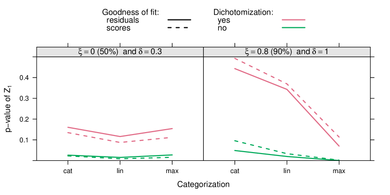
Figure 4: Effects of the three building blocks residuals vs. scores, dichotomization, and categorization in the “stump” scenario with the intercept and the slope parameter both varying. All possible combinations have been evaluated in two different settings and their performances are compared based on the mean $p$-values corresponding to the true split variable $Z_{1}$. Left panel: true split point at the median $0$ and with effect size $0.3$. Right panel: true split point at the $90$% quantile $0.8$ and with effect size $1$.

5.3 “Tree” scenario: Pre-pruning vs. post-pruning

So far the testing strategies underlying the different tree algorithms have only been considered as classical significance tests, i.e., in terms of power and $p$-values. However, one could argue that for a tree this is practically not really relevant – at least when combined with a post-pruning strategy such as cost-complexity pruning (Breiman et al., 1984). In the latter case it only matters that the relevant split variables have the lowest $p$-value among all potential split variables – but it is irrelevant whether this is significant or not. To investigate to which extent this is actually true we evaluate the different tree algorithms in the more complex “tree” scenario (see Figure 2): once with significance-based pre-pruning and once with cost-complexity post-pruning.

Recall that the true split structure is composed of splits in two different variables, both at the same split point $\xi$. First, the split in $Z_{2}$ changes the slope from $+\delta$ to $-\delta$. Second, the split in $Z_{1}$ changes the intercept in the negative slope group from $-\delta$ to $+\delta$. In the simulation the effect size $\delta$ is increased from 0 to 1 for different split points $\xi$ from 0 to 0.8. Here, the performance is not evaluated in terms of test properties but only in terms of tree properties, namely the adjusted Rand index (ARI) in comparison to the true partition of the data.

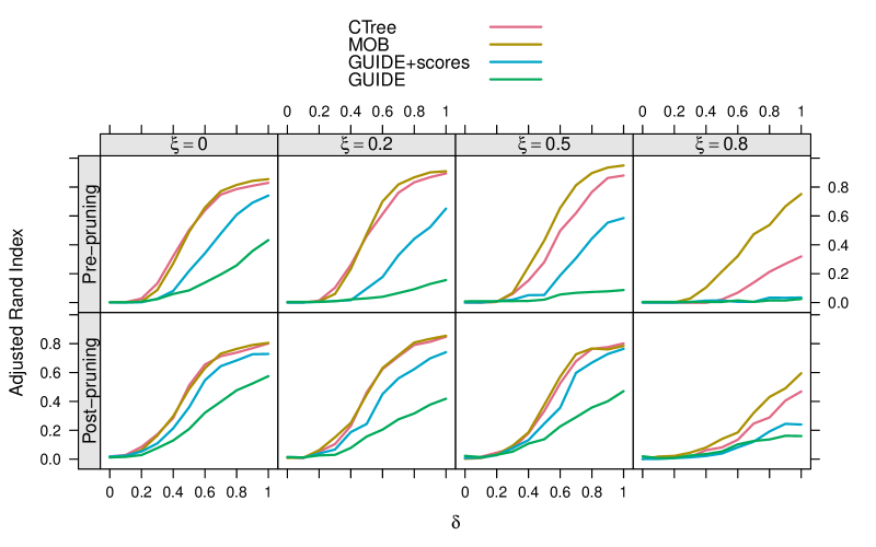
Figure 5: Adjusted Rand index (ARI) for the testing strategies CTree, MOB, GUIDE, and GUIDE+scores in the “tree” scenario, once applying pre-pruning (top row) and once post-pruning (bottom row). The ARI is evaluated over increasing effect size $\delta$ with 100 replications of 250 observations per step. Each panel represents a different value of the true split point $\xi$ ($0$, $0.2$, $0.5$ and $0.8$ from left to right, corresponding to the $50$%, $60$%, $75$%, and $90$% quantile).

The top row of Figure 5 presents the results for pre-pruning which, not surprisingly, reflect the results from previous sections. Thus, CTree and MOB perform similarly and rather well as the underlying significance tests have good power properties. Only for late abrupt shifts the linear test statistics in CTree clearly have lower power than the maximally-selected statistics in MOB. Again, this picture would reverse for smooth changes instead of abrupt shifts. Compared to CTree/MOB both GUIDE flavors clearly perform worse as the underlying tests are less powerful; notably for the residual-based GUIDE which again has problems picking up the slope change associated with $Z_{2}$.

When switching from pre-pruning to post-pruning (bottom row of Figure 5) it is indeed shown that many of the problems stemming from the low power of the two GUIDE flavors are indeed mitigated. Thus, by first growing a large tree without stopping upon non-significance and then pruning back based on predictive performance instead substantially improves the fit of the two GUIDE flavors. However, using the residuals only in GUIDE still performs clearly worse compared to the GUIDE+scores. The latter is essentially on par with CTree and MOB when the true split matches one of the categorization bins (i.e., $\xi=0$ and $\xi=0.5$, respectively) while CTree/MOB still perform somewhat better in the other cases ($\xi=0.2$ and $\xi=0.8$).

In summary, there is clear support for the conventional wisdom that the power of the testing strategy in an unbiased tree algorithm is not so important when combined with post-pruning. However, there are limits to this. Consequently, when tests can be made more powerful – e.g., by using scores instead of residuals – then this improves the corresponding tree algorithm. Finally, the simulation also supports using pre-pruning in an unbiased tree algorithm when the underlying testing strategy also works well as a classical significance test.

6 Discussion

The testing strategies underlying the unbiased recursive partitioning algorithms CTree, MOB, and GUIDE have been embedded in a common inference framework, highlighting what the tests have in common and what sets them apart. Concerning the effects of the corresponding building blocks for the tests, three main conclusions can be drawn:

• Goodness-of-fit measure: Assessing all dimensions of a model via the full scores is to be preferred over assessing only a subset with the residuals. The former can substantially improve performance while leading only to minor deteriorations when it is not necessary.

• Dichotomization of residuals/scores: No scenarios could be found where this is beneficial and tests without dichotomization performed clearly better in several scenarios.

• Categorization of split variables: The effects of categorization are not so clear-cut and depend on the true data structure. If there are indeed abrupt shifts close to the breaks from the categorization, it works well. However, for splits close to the margins performance can deteriorate and a maximally-selected test is preferable. Finally, a linear statistic performs better for smooth rather than abrupt changes.

Thus, also when categorization as in GUIDE is used we would recommend to employ the non-dichotomized scores instead of the dichotomized residuals. Note that such a test corresponds to a multiple ANOVAs (for the score components) and is easily available in statistical software. Moreover, in the R system the coin package provides a convenient toolbox that encompasses multivariate transformation functions $h$ and/or $g$.

Linear models as presented in this study have been chosen as they are highly relevant in practice, allow for simple illustrations, and theoretical insights are available for the testing strategies. However, the results can be easily extended to a wide variety of other models where the introduced building blocks can be applied in the same way. Specifically, it has been shown theoretically that certain changes in the parameters do not lead to shifts in the residuals (but in other components of the scores). Ploberger and Krämer (1992) showed that residual-based tests can detect a change in the parameters of a linear model only if it also causes a shift in the expected value $\mathbb{E}(Y)$. This is not the case if changes are orthogonal to the mean regressor which in our case is $(1,0)^{\top}$. Consequently, if only the slope $\beta_{1}$ but not the intercept $\beta_{0}$ changes, the shift is of type $(0,\delta)^{\top}$ and thus orthogonal to the mean regressor. Due to this residual-based tests as in GUIDE break down and do not have power to detect this. Note that this situation does not have to be rare in practice: Especially for binary regressor variables (e.g., as in treatment-subgroup investigations) it can easily occur (see Figure 2 in Loh et al., 2015, for an illustration).

Also in more general models, residual-based and score-based procedures are expected to perform equally well if all model parameters are highly correlated. But if parameters do change orthogonally this might again be missed when only considering residuals – and full model scores are typically easily available as the appropriate remedy. Note that the score function $s$ can also simply be seen as a transformation of the response variable $Y$ (and potentially regressors $X$) to a different space in order to allow for a well structured analysis of dependencies. This has been exploited in several tree-based approaches previously published in the literature, e.g., in Hothorn and Zeileis (2017) and Schlosser et al. (2019). Similarly, it would be of interest to investigate a score-based version of the extended GUIDE algorithms beyond the linear model, e.g., in Loh and Zheng, 2013, Chaudhuri and Loh, 2002, and Loh et al., 2015.

Computational details

The applied implementation is based on the R package partykit (version 1.2.4) which is available on R-Forge at https://R-Forge.R-project.org/projects/partykit/. The code to reproduce the simulation study is available in the supplement for this paper on arXiv.org E-Print Archive (https://arxiv.org/).

The functions ctree and mob provide an implementation of the two tree algorithms in their original form. For their adapted versions additional modifications have been applied within these functions allowing for a categorization of possible split variables and a dichotomization of scores. To evaluate the GUIDE algorithm a reimplementation of this algorithm has been built using the basic framework of ctree and mob.

Appendix A Test statistics

This section provides further information on the test statistics applied in CTree, MOB, and GUIDE. Most of the presented details have been extracted from the original papers Hothorn et al. (2006b), Zeileis et al. (2008), and Loh (2002), however, notation is adapted to the main manuscript in order to allow for better comparison.

A.1 CTree

To measure the association of a response $Y$ and each possible split variable $Z_{j}$, $j=1,\ldots,J$, the CTree algorithm applies a linear test statistic $T_{j}$ which is excerpted from Section 3.1. (“Variable selection and stopping criteria”) of the original paper (Hothorn et al., 2006b) and is of the following form:

$$T_{j}(Y,Z_{j},w)=\text{vec}\left(\sum_{i=1}^{N}w_{i}g_{j}(Z_{ji})h(Y_{i})^{\top}\right)$$

where $w$ are optional weights, $g_{j}:\mathcal{Z}_{j}\rightarrow\mathbb{R}^{P}$ is a nonrandom transformation of the split variable $Z_{j}$ and the influence function $h:\mathcal{Y}\times\mathcal{Y}^{N}\rightarrow\mathbb{R}^{Q}$ depends on the response $Y=(Y_{1},\ldots,Y_{N})$ in a permutation symmetric way and is set to $h(Y_{i})=s(Y_{i},X_{i},\hat{\beta})$ for a score-based approach. Moreover, by applying the “vec” operator the resulting $P~{}\times~{}Q$ matrix is converted into a $PQ$ column vector. Following Strasser and Weber (1999) the conditional expectation $\mu_{j}$ and covariance $\Sigma_{j}$ of a linear test statistic $T_{j}$ can be calculated and used to standardize an observed linear test statistic $t_{j}$ within a function $c$ mapping into the real line. For example, the maximum of the absolute values of the standardized linear statistic

$$c_{\max}(t_{j},\mu_{j},\Sigma_{j})=\max\left|\frac{(t_{j}-\mu_{j})}{\text{diag}(\Sigma_{j})}\right|$$

or a quadratic form

$$c_{\text{quad}}(t_{j},\mu_{j},\Sigma_{j})=(t_{j}-\mu_{j})\Sigma_{j}^{+}(t_{j}-\mu_{j})^{\top}$$

can be considered where $\Sigma_{j}^{+}$ is the Moore-Penrose inverse of $\Sigma_{j}$. Since the asymptotic conditional distribution of a linear test statistic $T_{j}$ is a multivariate normal with parameters $\mu_{j}$ and $\Sigma_{j}$ (Strasser and Weber, 1999), the asymptotic distribution of $c_{\text{max}}$ is normal while the quadratic form $c_{\text{quad}}$ follows an asymptotic $\chi^{2}$ distribution. Based on this knowledge the corresponding $p$-values can be calculated easily.

A.2 MOB

The MOB algorithm employs an empirical fluctuation process $W_{j}$ to measure deviations of the model scores $s$ from zero with respect to an ordering induced by the possible split variable $Z_{j}$, $j=1,\ldots,J$. As described in detail in Section 3.2. (“Testing for parameter instability”) of the original paper (Zeileis et al., 2008) this process is of the following form:

$$W_{j}(t)=\hat{V}^{-1/2}N^{-1/2}\sum_{i=1}^{\lfloor Nt\rfloor}s_{\pi(Z_{ji})}\qquad(0\leq t\leq 1)$$

with the model scores $s_{i}=s(Y_{i},X_{i},\hat{\beta})$ being sorted by the possible split variable $Z_{j}$ by including the ordering permutation $\pi(Z_{ji})$. To scale this partial sum process an estimate $\hat{V}$ of the covariance matrix $\text{cov}(s(Y,X,\hat{\beta}))$ is included. Following Zeileis and Hornik (2007) $W_{j}(t)$ converges to a Brownian bridge $W^{0}$ under the null hypothesis of parameter stability. To obtain a test statistic a scalar functional $\lambda(\cdot)$ capturing the fluctuation in the empirical process can be applied and the corresponding asymptotic distribution of $\lambda(W_{j}(t))$ can be obtained by employing the same functional to the limit process, i.e., $\lambda(W^{0})$.

One possible and intuitive choice for a functional in order to asses instabilities over a numerical split variable is the following:

$$\lambda_{\text{supLM}}(W_{j})=\max_{i=\underline{i},\ldots,\overline{i}}\left(\frac{i}{N}\cdot\frac{N-i}{N}\right)^{-1}\left|\left|W_{j}\left(\frac{i}{N}\right)\right|\right|_{2}^{2}$$

where a minimal segment size $\underline{i}$ and then $\overline{i}=N-\underline{i}$ are used to define the interval $[\underline{i},\overline{i}]$. Other possible functionals, for example also for categorical split variables, and more details, particularly on calculating the corresponding $p$-values can be found in Section 3.2. of the original paper (Zeileis et al., 2008).

A.3 GUIDE

The test statistic of the $\chi^{2}$ test as applied in the GUIDE algorithm is

$$X^{2}=\frac{(O_{11}-E_{11})^{2}}{E_{11}}+\ldots+\frac{(O_{24}-E_{24})^{2}}{E_{24}}$$

where $O_{lm}$ are the observed frequencies of observations in a certain combination of dichotomized residuals ($l=1,2$) and categorized split variables ($m=1,\ldots,4$). $E_{lm}$ are the corresponding expected frequencies under independence $E_{lm}=\frac{O_{l\cdot}\cdot O_{\cdot m}}{N}$. Under the null hypothesis of independence the asymptotic distribution of $X^{2}$ is a $\chi^{2}$ distribution allowing for a straight-forward calculation of $p$-values. If full model scores are used instead of residuals a sum of the test statistic over the number of distribution parameters is considered such that each summand corresponds to one column of the score matrix. For this case the degrees of freedom of the resulting $\chi^{2}$ distribution is then also the corresponding sum of degrees of freedom over the number of distribution parameters.

Appendix B Combinations of building blocks applied

For the evaluation of all 12 possible combinations of the presented building blocks the original testing strategies CTree, MOB, and GUIDE have been applied together with modified versions of them. The employed versions and the corresponding combination of building blocks are listed in Table 5.

Residuals/Scores	Dich.	Cat.	Via testing strategy
residuals	yes	cat	GUIDE	(default)
residuals	yes	max	MOB	(modified)
residuals	yes	lin	CTree	(modified)
residuals	no	cat	MOB	(modified)
residuals	no	max	MOB	(modified)
residuals	no	lin	CTree	(modified)
scores	yes	cat	GUIDE	(modified)
scores	yes	max	MOB	(modified)
scores	yes	lin	CTree	(modified)
scores	no	cat	MOB	(modified)
scores	no	max	MOB	(default)
scores	no	lin	CTree	(default)

Table 5: Testing strategies applied for all 12 factorial combinations of the building blocks. For each combination one of the three testing strategies CTree/MOB/GUIDE is applied, possibly after modifying the assessed variables as indicated (i.e., dichotomized or categorized).

Appendix C Significance level

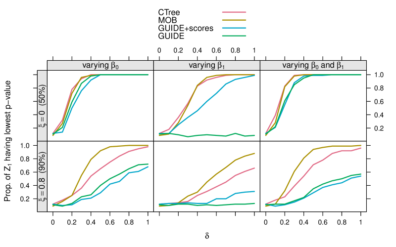
Figure 6: Proportion of replications where the true split variable $Z_{1}$ shows the smallest $p$-value, hence, where $Z_{1}$ is selected without any significance level in the “stump” scenario. The testing strategies CTree, MOB, GUIDE, and GUIDE+scores are evaluated over increasing effect size $\delta$ with 100 replications of 250 observations per step. The true split point in $Z_{1}$ is either the median 0 (top) or the 90% quantile 0.8 (bottom) for either varying intercept $\beta_{0}$ (left), varying slope $\beta_{1}$ (middle), or both coefficients varying (right).

In Section 5.1 the investigated testing strategies are compared based on the selection probability of $Z_{1}$, hence, the number of replications in which the true split variable $Z_{1}$ is detected with a $p$-value smaller than the predefined significance level $\alpha=0.05$. This choice of measurement is due to the aim of investigating how well the tests perform as significance test. However, ignoring this significance level yields the same conclusions which can be seen when comparing Figures 6 and 3, both being based on the exact same evaluation, but in Figure 6 the proportion of replications in which the true splitting variable $Z_{1}$ is detected by showing the smallest $p$-value, but not necessarily smaller than the significance level, is illustrated.

Appendix D Continuous “stump” scenario

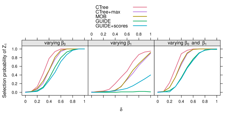
Figure 7: Selection probability of the true split variable $Z_{1}$ for testing strategies CTree, CTree+max, MOB, GUIDE, and GUIDE+scores for continuous parameter functions $\beta_{0}(Z_{1})$ and $\beta_{1}(Z_{1})$. Probabilities are estimated over increasing effect size $\delta$ with 100 replications of 250 observations per step. Each panel represents one variation for the coefficients: varying intercept $\beta_{0}$ (left), varying slope parameter $\beta_{1}$ (middle) and both coefficients varying (right).

In the simulation study presented in Sections 4 and 5 the intercept and slope parameters $\beta_{0}$ and $\beta_{1}$ are both either fixed or binary variables taking either the positive or the negative value of the effect size $\delta$. Therefore, these parameters are step functions for which the maximum selection employed in the testing strategy of MOB has shown to perform better than the linear selection in CTree. However, this changes in case of monotonous functions where CTree is advantageous as it is constructed to detect monotonous effects. To point out that the difference in performance of CTree and MOB depends on the type of effect the same setting for which the results are presented in Figure 3 is evaluated again but this time with the varying parameter(s) changing continuously. In particular, the parameters $\beta_{0}$ and $\beta_{1}$ are linear functions of the true split variable $Z_{1}$:

$$\beta_{k-1}(Z_{1})=\begin{cases}-\delta\cdot(-1)^{k-1}\cdot Z_{1}\\ +\delta\cdot(-1)^{k-1}\cdot Z_{1}\end{cases}$$

for $k=1,2=K$. Additionally, a modified version of CTree employing a maximum selection, such as MOB, is evaluated (denoted by CTree+max). Looking at the selection probability illustrated in Figure 7 it can be observed that in this setting the original version of CTree is ahead while CTree+max and MOB perform almost equally well. Hence, the comparison of Figures 3 and 7 points out that it clearly depends on the type of effect whether the maximum selection (MOB, CTree+max) or the linear selection (CTree) is to be preferred.

Appendix E Results for increasing effect size

E.1 Dichotomization of residuals/scores

To elaborate over an increasing effect size whether a dichotomization of the residuals/scores at zero leads to an improvement or a deterioration of performance, CTree and MOB are applied, once in their original version without dichotomization and once in an adapted version with a dichotomization of scores at zero (CTree+dich, MOB+dich). Moreover, they are compared to the adapted GUIDE version which includes all available scores (GUIDE+scores).

Figure 9 shows the effect of dichotomizing the score values over different values for the true split point $\xi$, however, all four situations lead to the same conclusions: Dichotomizing the score values decreases the selection probability of the true split variable $Z_{1}$, and hence reduces the power of the testing strategy.

E.2 Categorization of splitting variables

To investigate the effect of categorizing the possible splitting variables CTree and MOB are applied, once in their original version without a categorization and once in an adapted version with a categorization of the possible split variables (CTree+cat and MOB+cat). Moreover, they are also compared to GUIDE+scores which includes all available scores.

In Figure 9 the impact of categorizing split variables on the performance is illustrated by the selection probability of $Z_{1}$ over increasing effect size and for four different values of the true split point $\xi$. For both, CTree and MOB, it can be stated that overall they perform better in their original form without categorization. Only if the true split point $\xi$ is close to the quartiles used as breaks for the categorizations both versions lead to a selection probability of $Z_{1}$ (e.g., for CTree and $\xi=0.5$)

Therefore, these results support the conclusions drawn in the main manuscript: Categorizing the values of the split variable does not lead to any advantages unless the true split point corresponds (or is at least close) to one of the quartiles used for the categorization. In most situations it even causes the power of the testing strategy to decrease.

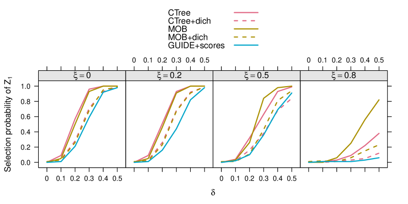
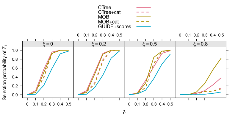
Figure 8: Selection probability of the true split variable $Z_{1}$ for testing strategies CTree, CTree+dich, MOB, MOB+dich, and GUIDE+scores in the “stump” scenario with both parameters varying. CTree+dich and MOB+dich refer to modifications of CTree and MOB applying a dichotomization of residuals/scores. Probabilities are estimated over increasing effect size $\delta$ with 100 replications of 250 observations per step. Each panel represents a different value of the true split point $\xi$ (0, 0.2, 0.5 and 0.8 from left to right corresponding to the 50%, 60%, 75%, and 90% quantile).

Figure 9: Selection probability of the true split variable $Z_{1}$ for testing strategies CTree, CTree+cat, MOB, MOB+cat, and GUIDE+scores in the “stump” scenario with both parameters varying. Probabilities are estimated over increasing effect size $\delta$ with 100 replications of 250 observations per step. Each panel represents a different value of the true split point $\xi$ (0, 0.2, 0.5 and 0.8 from left to right corresponding to the 50%, 60%, 75%, and 90% quantile).

References

- Breiman et al. (1984) Breiman L, Friedman JH, Olshen RA, Stone CJ (1984). Classification and Regression Trees. Wadsworth, California.
- Chaudhuri and Loh (2002) Chaudhuri P, Loh WY (2002). “Nonparametric Estimation of Conditional Quantiles Using Quantile Regression Trees.” Bernoulli, 8(5), 561–576. URL https://projecteuclid.org:443/euclid.bj/1078435218.
- Doyle (1973) Doyle P (1973). “The Use of Automatic Interaction Detector and Similar Search Procedures.” Operational Research Quarterly (1970-1977), 24(3), 465–467. URL http://www.jstor.org/stable/3008131.
- Fokkema et al. (2018) Fokkema M, Smits N, Zeileis A, Hothorn T, Kelderman H (2018). “Detecting Treatment-Subgroup Interactions in Clustered Data with Generalized Linear Mixed-Effects Model Trees.” Behavior Research Methods, 50(5), 2016–2034. 10.3758/s13428-017-0971-x.
- Grün et al. (2012) Grün B, Kosmidis I, Zeileis A (2012). “Extended Beta Regression in R: Shaken, Stirred, Mixed, and Partitioned.” Journal of Statistical Software, Articles, 48(11), 1–25. ISSN 1548-7660. 10.18637/jss.v048.i11.
- Hothorn et al. (2006a) Hothorn T, Hornik K, Van de Wiel MA, Zeileis A (2006a). “A Lego System for Conditional Inference.” The American Statistician, 60(3), 257–263. 10.1198/000313006X118430.
- Hothorn et al. (2006b) Hothorn T, Hornik K, Zeileis A (2006b). “Unbiased Recursive Partitioning: A Conditional Inference Framework.” Journal of Computational and Graphical Statistics, 15(3), 651–674. 10.1198/106186006x133933.
- Hothorn and Zeileis (2008) Hothorn T, Zeileis A (2008). “Generalized Maximally Selected Statistics.” Biometrics, 64(4), 1263–1269. 10.1111/j.1541-0420.2008.00995.x.
- Hothorn and Zeileis (2017) Hothorn T, Zeileis A (2017). “Transformation Forests.” arXiv 1701.02110, arXiv.org E-Print Archive. URL http://arxiv.org/abs/1701.02110.
- Kim and Loh (2001) Kim H, Loh WY (2001). “Classification Trees with Unbiased Multiway Splits.” Journal of the American Statistical Association, 96(454), 589–604. 10.1198/016214501753168271.
- Loh (2002) Loh WY (2002). “Regression Trees with Unbiased Variable Selection and Interaction Detection.” Statistica Sinica, 12(2), 361–386. URL http://www.jstor.org/stable/24306967.
- Loh et al. (2015) Loh WY, He X, Man M (2015). “A Regression Tree Approach to Identifying Subgroups with Differential Treatment Effects.” Statistics in Medicine, 34(11), 1818–1833. 10.1002/sim.6454.
- Loh and Shih (1997) Loh WY, Shih YS (1997). “Split Selection Methods for Classification Trees.” Statistica Sinica, 7(4), 815–840. URL http://www.jstor.org/stable/24306157.
- Loh and Vanichsetakul (1988) Loh WY, Vanichsetakul N (1988). “Tree-Structured Classification via Generalized Discriminant Analysis.” Journal of the American Statistical Association, 83(403), 715–725. 10.1080/01621459.1988.10478652.
- Loh and Zheng (2013) Loh WY, Zheng W (2013). “Regression Trees for Longitudinal and Multiresponse Data.” The Annals of Applied Statistics, 7(1), 495–522. 10.1214/12-AOAS596.
- Morgan and Sonquist (1963) Morgan JN, Sonquist JA (1963). “Problems in the Analysis of Survey Data, and a Proposal.” Journal of the American Statistical Association, 58(302), 415–434. 10.1080/01621459.1963.10500855.
- Ploberger and Krämer (1992) Ploberger W, Krämer W (1992). “The CUSUM Test with OLS Residuals.” Econometrica, 60(2), 271–285. 10.2307/2951597.
- Schlosser et al. (2019) Schlosser L, Hothorn T, Stauffer R, Zeileis A (2019). “Distributional Regression Forests for Probabilistic Precipitation Forecasting in Complex Terrain.” arXiv 1804.02921, arXiv.org E-Print Archive. URL http://arxiv.org/abs/1804.02921.
- Seibold et al. (2016) Seibold H, Zeileis A, Hothorn T (2016). “Model-Based Recursive Partitioning for Subgroup Analyses.” The International Journal of Biostatistics, 12(1), 45–63. 10.1515/ijb-2015-0032.
- Strasser and Weber (1999) Strasser H, Weber C (1999). “On the Asymptotic Theory of Permutation Statistics.” Mathematical Methods of Statistics, 8, 220–250.
- Strobl et al. (2015) Strobl C, Kopf J, Zeileis A (2015). “Rasch Trees: A New Method for Detecting Differential Item Functioning in the Rasch Model.” Psychometrika, 80(2), 289–316. 10.1007/s11336-013-9388-3.
- Su et al. (2004) Su X, Wang M, Fan J (2004). “Maximum Likelihood Regression Trees.” Journal of Computational and Graphical Statistics, 13(3), 586–598. 10.1198/106186004X2165.
- Zeileis and Hornik (2007) Zeileis A, Hornik K (2007). “Generalized M-Fluctuation Tests for Parameter Instability.” Statistica Neerlandica, 61(4), 488–508. 10.1111/j.1467-9574.2007.00371.x.
- Zeileis and Hothorn (2013) Zeileis A, Hothorn T (2013). “A Toolbox of Permutation Tests for Structural Change.” Statistical Papers, 54(4), 931–954. 10.1007/s00362-013-0503-4.
- Zeileis et al. (2008) Zeileis A, Hothorn T, Hornik K (2008). “Model-Based Recursive Partitioning.” Journal of Computational and Graphical Statistics, 17(2), 492–514. 10.1198/106186008x319331.