The Finite-Horizon Two-Armed Bandit Problem
with Binary Responses
 
A Multidisciplinary Survey of the History, State of the Art, and Myths

Abstract

In this paper we consider the two-armed bandit problem, which often naturally appears per se or as a subproblem in some multi-armed generalizations, and serves as a starting point for introducing additional problem features. The consideration of binary responses is motivated by its widespread applicability and by being one of the most studied settings. We focus on the undiscounted finite-horizon objective, which is the most relevant in many applications. We make an attempt to unify the terminology as this is different across disciplines that have considered this problem, and present a unified model cast in the Markov decision process framework, with subject responses modelled using the Bernoulli distribution, and the corresponding Beta distribution for Bayesian updating. We give an extensive account of the history and state of the art of approaches from several disciplines, including design of experiments, Bayesian decision theory, naive designs, reinforcement learning, biostatistics, and combination designs. We evaluate these designs, together with a few newly proposed, accurately computationally (using a newly written package in Julia programming language by the author) in order to compare their performance. We show that conclusions are different for moderate horizons (typical in practice) than for small horizons (typical in academic literature reporting computational results). We further list and clarify a number of myths about this problem, e.g., we show that, computationally, much larger problems can be designed to Bayes-optimality than what is commonly believed.

Keywords: Multi-armed bandit problem; Design of sequential experiments; Bayesian decision theory; Dynamic programming; Index rules; Response-adaptive randomization;

1 Introduction

Statistical testing based on randomized equal allocation is a widespread state-of-the-art approach in the design of experiments for around $100$ years, known today as the randomized controlled trial in biostatistics, the between-group design in social sciences, and the A/B testing in digital marketing. Already Thompson, (1933), a biostatistician from Yale University, proposed a data-driven approach which would in expectation lead to a higher reward from an experiment, using the following words:

“…there can be no objection to the use of data, however meagre, as a guide to action required before more can be collected … Indeed, the fact that such objection can never be eliminated entirely—no matter how great the number of observations—suggested the possible value of seeking other modes of operation than that of taking a large number of observations before analysis or any attempt to direct our course…”

Robbins, (1952), a prominent mathematician and statistician, emphasized that this problem is of a much wider importance:

“In fact, the problem represents in a simplified way the general question of how we learn—or should learn—from past experience.”

A formulation of the problem using the Bayesian decision-theoretic framework allows for Bayes-optimality. Practical application of this Bayesian approach has however been long hindered by its computational complexity, since the optimal solution is known in analytical form only for infinite horizon (Kelly,, 1981). A variety of practical approximations and heuristics have been developed and studied across several disciplines in order to overcome this issue, but their analysis failed to give exact results or bounds sufficiently close to Bayes-optimality for finite horizon problems, which are the problems most relevant to many situations in practice.

1.1 Paper Structure and Contributions

In this paper we thus focus on the finite-horizon setting. We also restrict the discussion to two arms, which often naturally appears per se or as a subproblem in some multi-armed generalizations (e.g. if new arms appear over time), and serves as a starting point for introducing additional problem features. The consideration of binary responses is motivated by its widespread applicability and by being one of the most studied settings.

Our main objective is to give an account of modelling and solution approaches arising in different disciplines, in a unified framework and using a unified terminology. The problem description, origins and terminology is given in Section 2. Our unified model is described in Section 3, cast in the Markov decision process framework, with subject responses modelled using the Bernoulli distribution, and the corresponding Beta distribution for Bayesian updating. Different problem settings, assumptions and objectives are summarized in Section 4. Section 5 gives an account of the history and state of the art of approaches from several disciplines. In Section 6 we evaluate these designs, together with a few newly proposed, accurately computationally (using a newly written package in Julia programming language by the author) in order to compare their performance, showing that conclusions are different for moderate horizons (typical in practice) than for small horizons (typical in academic literature reporting computational results). We further list and clarify a number of myths about this problem in Section 7, e.g., we show that, computationally, much larger problems can be designed to Bayes-optimality than what is commonly believed. Section 8 concludes.

2 Problem

We consider the problem with two arms (or, interventions), called $C$ (mnemonically for “control” or “comparator” or standard of “care”) and $D$ (for “discovery” or “development”). $T$ subjects become available one by one, and each subject must be allocated to exactly one of the arms. Upon allocation of a subject to arm $C$ ($D$), subject’s response is observed, which is binary (success/failure), where the success probability is $\theta_{C}$ ($\theta_{D}$) and the failure probability is $1-\theta_{C}$ ($1-\theta_{D}$). The primary objective is to find a design, i.e. a strategy composed of randomized actions of allocating the subjects to arms, which, in expectation, achieves the highest number of observed successes from the $T$ subjects, assuming that the success probabilities are unknown. A formal model is given in Section 3.

2.1 Problem Origins

The first statement of the two-armed bandit problem is in Thompson, (1933), extended in Thompson, (1935) to multiple arms, in a Bayesian setting. Apparently unaware of Thompson’s works, Robbins, (1952) formulated the two-armed bandit problem in a frequentist setting. Neither Thompson, (1933, 1935) nor Robbins, (1952) used the terms “arm” or “bandit”. The term two-armed bandit problem first appeared in Bradt et al., (1956), referring to the setting with binary responses in which one knows the set $\{\theta_{C},\theta_{D}\}$, but does not know which arm is which. Bradt et al., (1956) also proposed a generalization of that problem, in which $\{\theta_{C},\theta_{D}\}$ is unknown, which is the two-armed bandit problem as known today and as considered in this paper. Bellman, (1956) referred to the latter problem as the two-machine problem.

P. Whittle stated on several occasions that researchers were aware of this type of problem since the 1940s and considered it an important but very hard open problem. That could be attributed to the absence of a suitable mathematical framework and theory, as the progress on the problem occurred slowly alongside the emergence and the development of areas such as sequential analysis, Bayesian statistics, decision theory, dynamic programming, stochastic processes, and concentration inequalities.

Indeed, early papers describing theoretical solutions on the bandit problem were often among the pioneers in these areas, introducing novel terminology and notation, not all of which has been adopted more generally, and might thus be hard to read for today’s researchers. Drawing on the early research in 1950s and 1960s, three dominant “schools” have emerged:

• the Berry’s school: starting with Berry, (1972), and rewritten and further developed in Berry and Fristedt, (1985), focussing predominantly on the finite-horizon setting;

• the Gittins’ school: starting with Gittins and Jones, (1974), and rewritten and further developed in Gittins, (1979, 1989); Gittins et al., (2011), focussing predominantly on the discounted infinite-horizon setting;

• the Robbins’ school: starting with Lai and Robbins, (1985), and rewritten and further developed in Agrawal, (1995); Katehakis and Robbins, (1995); Burnetas and Katehakis, (1996), focussing predominantly on the time-average infinite-horizon setting.

The author’s suggestion is that this pioneering literature should be on the must-read list of researchers on bandit problems, regardless of their discipline.

While the Robbins’ school makes complete learning (i.e. identification of the better arm in infinite time almost surely) lexicographically more important than the way of attaining it, both the Berry’s and Gittins’ schools replace the lexicographic ordering by resolving the trade-off between complete learning and earning (of rewards), with the relative weights implicitly given by the horizon and the discount factor, respectively. In Section 5 we describe these “schools” and their relationships in more detail.

Of course, there are several other fascinating variants of the bandit problem, with different objective (e.g., risk-averse, adversarial, final-period-only, etc.), different control (e.g., randomized, multi-mode, multi-resource, duelling, multi-player, etc.), and/or different dynamics (e.g., non-binary responses, delayed responses, partial observability, arriving arms, covariates, correlation, restlessness, non-stationarity, non-Markovian, etc.); all these are unfortunately beyond the scope of this paper.

2.2 Applications

The problem has been formulated, addressed or applied in a number of disciplines, each developing its own terminology, see Table 1. In this paper we use the terminology which we believe is a reasonable compromise and should not cause confusion for researches and practitioners from all the disciplines. The author wishes to encourage researchers from all the disciplines to follow this terminology as closely as possible to facilitate for researchers and practitioners from other disciplines to learn about their work.

According to Scott, (2010): “Multi-armed bandits have an important role to play in modern production systems that emphasize continuous improvement, where products remain in a perpetual state of feature testing even after they have been launched.” The most commonly listed applications, often requiring to adapt the generic multi-armed bandit problem to specific features, are as follows:

• Digital marketing: In the digital world it is relatively easy to introduce and quick to get feedback on new document variants, and so bandit problems have been proposed for social media advertising, personalized websites and user interfaces, email campaigns, influence maximization, etc; see, e.g., Liberali et al., (2017). Bandit problems can also be used to address the problem of dynamic pricing with demand uncertainty, which requires to solve a trade-off of learning (of the demand curve) and earning (the highest revenue); for a survey, see, e.g., den Boer, (2015).

• Clinical trials: Thompson, (1933) pointed out that his bandit problem “…would be important in cases where either the rate of accumulation of data is slow or the individuals treated are valuable, or both.” Gluss, (1962) further explained the motivation primarily by rare diseases. Following the focus on rare and/or life-threatening diseases, a few novel bandit-based designs have been developed and proposed recently, and are being implemented in a growing number of trials, mainly in several types of cancer, where patients are stratified into smaller groups using genetic biomarkers. Discussions about the advantages and disadvantages of bandit-based designs are ongoing, e.g., Berry and Esserman, (2016) argue that, in certain clinical trials, data-driven approaches make great sense ethically, statistically, economically, scientifically, and logistically. For a survey on real adaptive trials, see e.g., Bothwell et al., (2018).

• Search: Bandit designs have been proposed for recommender systems in which new items and users appear frequently in order to assure sufficient exploration, see, e.g., Aggarwal, (2016). Although digital search is typically considered by recommender systems, many non-digital search applications exist, e.g. search for natural resources, search and rescue, surveillance and monitoring. Related to this category are also the so-called best-arm identification problem and problems appearing in ranking and selection.

Anecdotic	strategy	choice	pull	arms
Operations & Management	policy	allocation	resource	projects
Reinforcement learning	algorithm	decision	time step	actions
Biometrics & Biostatistics	design	randomization	patient	treatments
Ranking & selection	policy	spread over	measurement	alternatives
Economics	strategy	choice	resource	experiments
Computing & Telecom.	scheduler	allocation	server	jobs
Marketing	policy	allocation	impression	advertisements
Transportation	driver	selection	vehicle	roads
This paper	design	randomized action	subject	interventions/arms

Table 1: An illustration of typical terminology for bandit problems across disciplines

3 Model

In this section we formulate a general two-armed problem with binary responses as a Markov decision process, which provides sufficient generality to accommodate all the solution approaches discussed in Section 5.

Interventions.

We consider arms (or, interventions) labelled by $k\in\mathcal{K}:=\{C,D\}$. A subject must be allocated to exactly one intervention, and such allocation yields a binary response from that intervention: $0$ (failure) or $1$ (success). The response set is denoted by $\mathcal{O}:=\{0,1\}$. Subject responses are uncertain, i.e., modelled as Bernoulli-distributed with parameter $0\leq\theta_{k}\leq 1$, the success probability, independent across arms. The responses are immediate, meaning that the response of an allocated subject is observed before the next decision needs to be done.

Timing.

Subjects arrive (i.e., are recruited) sequentially (i.e., one by one) at random moments in continuous time. Since we do not discount the future, we can without loss of generality focus only on the moments of subjects’ arrivals, which we call discrete time epochs and see as regularly spaced. That is, equivalently, we can consider that subjects arrive at time epochs $t\in\mathcal{T}:=\{0,1,2,\dots,T-1\}$, where $T\leq+\infty$ is the number of subjects in the trial, i.e., the trial size, or the time horizon. To clarify, the $(t+1)$-st subject arrives at time epoch $t$. Note that $t=T$ is the time epoch denoting the end of the trial, when the response of the last subject is observed and no subject arrives.

States.

At any moment in continuous time, the physical state is represented by the numbers of observed successes and failures on each arm, the number of allocated subjects without an observed response on each arm, the number of arrived subjects without being allocated, and the number of remaining subjects to arrive. This is a vector with $8$ elements summing up to $T$ at any moment (all are non-negative integers). At time epochs, this can be simplified without loss of generality to a vector with $5$ elements, with the numbers of observed successes and failures on arm $C$ denoted by $s_{C}$ and $f_{C}$, respectively, the numbers of observed successes and failures on arm $D$ denoted by $s_{D}$ and $f_{D}$, respectively, and the number of remaining subjects to be allocated (exactly one of which has arrived), $n$. Since at time epochs $s_{C}+f_{C}+s_{D}+f_{D}+n=T$, it is sufficient to keep track of any four of these five numbers, leading to a state as vector with $4$ elements, which we choose to be $\boldsymbol{x}:=(s_{C},f_{C},s_{D},f_{D})$. Note that at time epoch $t$, $s_{C}+f_{C}+s_{D}+f_{D}=t$.

In addition to the physical state, there is an information state, which at any moment in continuous time captures all the information that could possibly affect the decisions. This may include real-world evidence and/or modelling assumptions. The real world evidence may be available before the start and/or it can arrive anytime during the trial. The modelling assumptions typically refer to the parameters of the prior distributions (built on historical data or expert opinions) for the success probability of each arm (whose weight may change over time, and can be either informative or non-informative), but may also include other parameters such as the probability of dropouts, the probability of errors in recording the observations and/or the subject allocations, the probability of mistakes in the statistical analysis and/or in the administration process, the timing of planned interim analyses, the probability and/or timing of unplanned stopping of the trial due to safety concerns, the estimate of the size of the subject population after the end of the trial, etc. For full generality, we consider the information state $\boldsymbol{i}$ (potentially dependent on the current physical state $\boldsymbol{x}$ and/or otherwise changing during the trial), and thus the state is $(\boldsymbol{x},\boldsymbol{i})$.

Actions.

At every time epoch $t\in\mathcal{T}$ the design must prescribe how the arrived subject should be randomized (i.e., randomly allocated) to interventions. While there are only two possible allocations, in every state we consider a possibly infinite action set $\mathcal{A}_{(\boldsymbol{x},\boldsymbol{i})}$ of randomized actions $a$ identified by probabilities $(p_{C}^{a},p_{D}^{a})$, meaning that the subject is allocated to intervention $C$ ($B$) with probability $p_{C}^{a}$ ($p_{D}^{a}$). Formally, $\mathcal{A}_{(\boldsymbol{x},\boldsymbol{i})}\subseteq\{a:p_{C}^{a}\geq 0,p_{D}^{a}\geq 0,p_{C}^{a}+p_{D}^{a}=1)\}.$ Since from the theory of Markov decision processes it follows that an action which is a randomized combination of other two actions is optimal only if all three are optimal, it is sufficient to consider only an action set of two pure randomized actions, which we call action $1$ (identified by $(p_{C}^{1},p_{D}^{1})$) and action $2$ (identified by $(p_{C}^{2},p_{D}^{2})$). For convenience in situations when both actions are optimal, we also consider an equally-weighted mixed randomized action, which we call action $3$ (identified by $(p_{C}^{3},p_{D}^{3}):=((p_{C}^{1}+p_{C}^{2})/2,(p_{D}^{1}+p_{D}^{2})/2)$), which is a combination of the two pure randomized actions with equal weights. Formally, $\mathcal{A}_{(\boldsymbol{x},\boldsymbol{i})}=\{1,2,3\}$, and without loss of generality we assume $p_{C}^{1}\geq p_{C}^{2}$. In some approaches discussed in Section 5, there is no choice of actions, meaning that the cardinality of $\mathcal{A}_{(\boldsymbol{x},\boldsymbol{i})}$ is one, which can be obtained by setting $1\equiv 2\equiv 3$, effectively reducing the Markov decision process to a Markov reward process.

In some approaches, the action set depends on the observations only via their sum $t=s_{C}+f_{C}+s_{D}+f_{D}$, thus can be written as $\mathcal{A}(t)$. Finally, the simplest case is the one in which the action set is constant, which we write as $\mathcal{A}$.

Transition Probabilities.

Denote by $q_{k,(\boldsymbol{x},\boldsymbol{i}),o}$ the probability of observing response $o\in\mathcal{O}$ for the current subject if it is allocated to arm $k\in\mathcal{K}$ in state $(\boldsymbol{x},\boldsymbol{i})$. We assume that $\sum_{o\in\mathcal{O}}q_{k,(\boldsymbol{x},\boldsymbol{i}),o}=1$ for all $k$, but this can be relaxed in some models, e.g. if allowing for dropouts (i.e., missing responses).

If the information state $\boldsymbol{i}$ does not change during the trial, then the transition probabilities of moving from state $(\boldsymbol{x},\boldsymbol{i})$ to state $(\boldsymbol{x}^{\prime},\boldsymbol{i})$ under action $a$ are

$$h_{(\boldsymbol{x},\boldsymbol{i}),(\boldsymbol{x}^{\prime},\boldsymbol{i})}^{a}=\begin{cases}p_{C}^{a}q_{C,(\boldsymbol{x},\boldsymbol{i}),1}&\text{ if }\boldsymbol{x}^{\prime}=\boldsymbol{x}+\boldsymbol{e}_{1}\\ p_{C}^{a}q_{C,(\boldsymbol{x},\boldsymbol{i}),0}&\text{ if }\boldsymbol{x}^{\prime}=\boldsymbol{x}+\boldsymbol{e}_{2}\\ p_{D}^{a}q_{D,(\boldsymbol{x},\boldsymbol{i}),1}&\text{ if }\boldsymbol{x}^{\prime}=\boldsymbol{x}+\boldsymbol{e}_{3}\\ p_{D}^{a}q_{D,(\boldsymbol{x},\boldsymbol{i}),0}&\text{ if }\boldsymbol{x}^{\prime}=\boldsymbol{x}+\boldsymbol{e}_{4}\\ \end{cases}$$

where $\boldsymbol{e}_{j}$ is the standard basis vector. If the information state changes during the trial, then these transition probabilities need to be amended to reflect its dynamics.

Expected One-Period Rewards.

The expected one-period reward $r_{(\boldsymbol{x},\boldsymbol{i})}^{a}$ for all states $(\boldsymbol{x},\boldsymbol{i})$ and all actions $a$ needs to be defined. If the information state $\boldsymbol{i}$ does not change during the trial, then it is as follows: $r_{(\boldsymbol{x},\boldsymbol{i})}^{a}=0$ for all states such that $s_{C}+f_{C}+s_{D}+f_{D}\leq T-1$ and $r_{(\boldsymbol{x},\boldsymbol{i})}^{a}=s_{C}+s_{D}$ for all states such that $s_{C}+f_{C}+s_{D}+f_{D}=T$ (i.e., the reward is the number of observed successes in all states in which the trial can eventually end).

The above definition of the reward is novel. The conventional one is to set the reward to the expected value of observing one success in a given state under a given action, i.e., $r_{(\boldsymbol{x},\boldsymbol{i})}^{a}=p_{C}^{a}q_{C,(\boldsymbol{x},\boldsymbol{i}),1}+p_{D}^{a}q_{D,(\boldsymbol{x},\boldsymbol{i}),1}$ at all time epochs $t=0,1,\dots,T-1$ and $r_{(\boldsymbol{x},\boldsymbol{i})}^{a}=0$ at time epoch $t=T$. In Appendix B we prove the following theorem.

Theorem 1.

The two reward definitions give the same expected total reward for any fixed design.

State and Action Processes.

The evolution of a Markov decision process is captured by the state process, which in full generality is 2-dimensional in order to keep the physical and information states separately, $(\boldsymbol{X}(\cdot),\boldsymbol{I}(\cdot))$, and the action process which depends on the state process, but can be briefly written as $A(\cdot)$, where $A_{(\boldsymbol{X}(t),\boldsymbol{I}(t))}\in\mathcal{A}_{(\boldsymbol{X}(t),\boldsymbol{I}(t))}$.

4 Assumptions, Settings and Objectives

4.1 Usage

There are three principal types of usage of the model described above.

Evaluation by Simulation.

Computer simulation is now a commonly used evaluation tool as it is relatively straightforward and the accuracy vs runtime trade-off can be addressed by adjusting the number of simulation runs. But we believe that it has the law-of-the-hammer syndrome of all simple universal tools: “if the only tool you have is a hammer, to treat everything as if it were a nail.”

Evaluation by Backward Recursion.

In this paper, we give evidence that it is possible and preferable to use backward recursion instead of simulation for evaluation. This yields a perfectly accurate evaluation (subject to computational accuracy of the chosen numerical type). We discuss its runtime in Section 7.

Optimization.

When the action set is not singular in all states, there is room for choosing one of the actions for every state according to an objective of maximizing some function. This does not necessarily need to be done by backward recursion; we describe several approaches in Section 5. In this case we assume that the success probabilities are unknown as otherwise it is trivial to optimize.

4.2 Knowledge Assumptions

While the success probabilities are assumed unknown for optimization, they may not necessarily be so for evaluation. There are two principal ways of specifying the probabilities $q_{k,(\boldsymbol{x},\boldsymbol{i}),o}$ of observing response $o$, which depend on the knowledge assumption about the success probabilities.

Known Success Probabilities.

Evaluation of all the approaches described in Section 5 can be done by assuming that success probabilities $\theta_{k}$ are known, and part of $\boldsymbol{I}(t)$ for all $t$. In that case the transition probabilities are independent of the physical state, so we can write $q_{k,\boldsymbol{i},o}$. If the information state is $\boldsymbol{i}=(\theta_{C},\theta_{D})$ during the whole trial, then

$$q_{k,\boldsymbol{i},o}=\begin{cases}\theta_{k}&\text{ if }o=1\\ 1-\theta_{k}&\text{ if }o=0\\ \end{cases}$$

Unknown Success Probabilities.

Approaches that allow for optimization assume that the success probabilities are unknown (otherwise the decision with the objective of maximising the expected number of successes is trivial), and so require estimates of these, which can be obtained using Bayesian updating. Following the existing literature, we use the Bayesian Beta-Bernoulli model for each arm $k\in\mathcal{K}$, in which $\theta_{k}$ is assumed to be a random variable drawn from Beta distribution dependent on the state. At the initial time epoch $t=0$, i.e., in physical state $(0,0,0,0)$, each arm $k$ is given a prior Beta distribution with parameters $\widetilde{s}_{k}(0),\widetilde{f}_{k}(0)$. These parameters can be interpreted as the numbers of pseudo-observations of successes and failures before the start of the trial. They are thus part of the information state $\boldsymbol{I}(t)$ for all $t$ and do not change over time. At every time epoch $t$, in physical state $\boldsymbol{x}=(s_{C},f_{C},s_{D},f_{D})$, each arm $k$ has the posterior distribution given, because of conjugacy, by the Beta distribution with parameters $\widetilde{s}_{k},\widetilde{f}_{k}$, briefly $\text{Beta}(\widetilde{s}_{k},\widetilde{f}_{k})$, where $\widetilde{s}_{k}=\widetilde{s}_{k}(0)+s_{k}$ and $\widetilde{f}_{k}=\widetilde{f}_{k}(0)+f_{k}$.

If the information state is $\boldsymbol{i}=(\widetilde{s}_{C}(0),\widetilde{f}_{C}(0),\widetilde{s}_{D}(0),\widetilde{f}_{D}(0))$ during the whole trial, then

$$q_{k,(\boldsymbol{x},\boldsymbol{i}),o}=\begin{cases}\frac{\widetilde{s}_{k}}{\widetilde{s}_{k}+\widetilde{f}_{k}}&\text{ if }o=1\\ \frac{\widetilde{f}_{k}}{\widetilde{s}_{k}+\widetilde{f}_{k}}&\text{ if }o=0\\ \end{cases}$$

The conventional assumption is to take the uniform distribution as a prior distribution on each arm $k$, i.e., $(\widetilde{s}_{k}(0),\widetilde{f}_{k}(0))=(1,1)$; for a discussion on choosing a different prior Beta distribution, see Appendix A.

4.3 Performance Measures and Objectives

In this paper we focus on the number of successes as the principal performance measure (a.k.a. operating characteristic in clinical trials literature). But instead of the number of successes, we report two equivalent measures: the proportion of successes and the regret number of successes, as these provide complementary interpretation and insights. Yet another equivalent measure (not reported in this paper) is the fraction of subjects allocated to the better arm. Many other additive measures, e.g. monetary cost typical in health economics and health technology assessment, can be defined analogously, but are not discussed in this paper.

A particular design $\pi$ prescribes the action process $A(\cdot)$. Let $\Pi$ be the set of designs that are non-anticipating and satisfy the above constraints on $A(\cdot)$.

Let us denote by $\operatorname{\mathbb{E}}^{\pi}_{t}[\cdot]$ the expectation under design $\pi\in\Pi$ conditioned on information available at time epoch $t\in\mathcal{T}$. The mean number of successes is

$$\mathbb{N}^{\pi}_{t}\left(\boldsymbol{x},\boldsymbol{i}\right):=\operatorname{\mathbb{E}}^{\pi}_{t} \left[\left.\sum_{u=t}^{T}r_{(\boldsymbol{X}(u),\boldsymbol{I}(u))}^{A_{(\boldsymbol{X}(u),\boldsymbol{I}(u))}}\right|\left(\boldsymbol{X}(t),\boldsymbol{I}(t)\right)=\left(\boldsymbol{x},\boldsymbol{i}\right)\right].$$ (1)

and the mean proportion of successes is

$$\mathbb{P}^{\pi}_{t}\left(\boldsymbol{x},\boldsymbol{i}\right):=\frac{1}{T-t}\mathbb{N}^{\pi}_{t}\left(\boldsymbol{x},\boldsymbol{i}\right).$$ (2)

These two are measures of subject benefit, while the former is on the absolute scale, the latter yields the average per-subject probability of observed success, i.e., the subject benefit on the percentage scale. We further define the mean regret number of successes,

$$\mathbb{R}^{\pi}_{t}\left(\boldsymbol{x},\boldsymbol{i}\right):=\operatorname{\mathbb{E}}\left[\left.\max\{\theta_{C},\theta_{D}\}\right|\boldsymbol{I}(t)=\boldsymbol{i}\right]-\mathbb{N}^{\pi}_{t}\left(\boldsymbol{x},\boldsymbol{i}\right),$$ (3)

which is a measure of subject loss. Note that all the three measures depend on parameter $T$, although we have suppressed the explicit notation.

The objective is to find an optimal design $\pi^{*}$ that maximises the mean number of successes as evaluated at time epoch $t=0$ when there are no observations ($\boldsymbol{x}=\boldsymbol{0}$), i.e.,

$$\pi^{*}:=\operatorname*{arg\,max}_{\pi\in\Pi}\mathbb{N}^{\pi}_{0}\left(\boldsymbol{0},\boldsymbol{i}\right)$$ (4)

or, equivalently, maximizes the mean proportion of successes, or, equivalently, minimizes the mean regret number of successes.

Following the two knowledge assumptions above, we have two approaches to performance evaluation.

Known Success Probabilities.

When the success probabilities are assumed to be known, we call the above measures the frequentist number of successes, the frequentist proportion of successes, and the frequentist regret number of successes, respectively. Due to symmetry, we can assume that $\theta_{C}\leq\theta_{D}$ without loss of generality, and thus

$$\mathbb{R}^{\pi}_{t}\left(\boldsymbol{x},\boldsymbol{i}\right)=\theta_{D}-\mathbb{N}^{\pi}_{t}\left(\boldsymbol{x},\boldsymbol{i}\right).$$ (5)

Unknown Success Probabilities.

When the success probabilities are assumed to be unknown, we evaluate performance in terms of the quantities known in the literature as the Bayes return, Bayes worth, or Bayes risk. In particular, we call the above measures the Bayes number of successes, the Bayes proportion of successes, and the Bayes regret number of successes, respectively.

For a problem with uniform distribution as a prior distribution on each arm, as considered in this paper, $\operatorname{\mathbb{E}}\left[\left.\max\{\theta_{C},\theta_{D}\}\right|\boldsymbol{I}(t)=\boldsymbol{i}\right]=2/3$ (Berry,, 1978), thus

$$\mathbb{R}^{\pi}_{t}\left(\boldsymbol{x},\boldsymbol{i}\right)=\frac{2}{3}-\mathbb{N}^{\pi}_{t}\left(\boldsymbol{x},\boldsymbol{i}\right),$$ (6)

Note that our definition is different from the so-called Bayesian regret (cf. Lattimore and Szepesvári,, 2019, Section 34.6), which is the average of the frequentist regret with respect to the prior distribution, i.e. it is Bayesian only in the initial time epoch.

5 Approaches

In this section we describe a number of common approaches to the problem described in the previous section. We start with Equal Randomized Allocation, which was originally developed for static setting, in which all the subjects arrive at the same time. All the remaining approaches are suitable only in dynamic setting, i.e., are data-driven.

5.1 Design of Experiments

Statistical testing based on equal (i.e., 1:1) randomized allocation (a.k.a. random assignment) is a widespread state-of-the-art approach in the design of experiments today, known as randomized controlled trial in medicine, between-group design in social sciences, and A/B testing in digital marketing. I theory, it allows the greatest reliability and validity of statistical estimate of the intervention effect (i.e., the difference between the two success probabilities) under an initial equipoise assumption. Originally developed, advocated and popularized by the founders of statistics such as C. S. Peirce in the fields of psychology and education in the late 19th century, and J. Neyman and R. A. Fisher in agriculture and other fields in the early 20th century. In the middle of the 20th century, A. B. Hill popularized the method in the field of medicine and it is now the preferred approach by regulatory agencies for assessing efficacy when deciding about marketing authorisation of new medicinal interventions in many countries. The approach can be evaluated using routine (frequentist) statistical methods.

In this approach the transition probabilities are frequentist, and

• the information state $\boldsymbol{i}$ is ignored;

• the action set is constant, $|\mathcal{A}|=1$ and $p_{C}^{a}=p_{D}^{a}=1/2$;

If the success probabilities are known, then its performance can be evaluated directly: the proportion of successes with mean $(\theta_{C}+\theta_{D})/2$ and standard deviation $\sqrt{(\theta_{C}+\theta_{D})(2-\theta_{C}-\theta_{D})/4T}$; the regret number of successes with mean $T\max\{(\theta_{C}-\theta_{D})/2,(\theta_{D}-\theta_{C})/2\}$ and standard deviation $\sqrt{T(\theta_{C}+\theta_{D})(2-\theta_{C}-\theta_{D})/4}$.

The approach is believed to be well understood. However, there are several potential concerns, e.g., (i) it was developed under the assumption of an infinite population of subjects to which the best arm will be applied, but it is not clear how valid it is when the population is finite or when new, potentially better arms become available in future; (ii) it was developed under the assumption of parallel allocation of subjects, but in dynamic (i.e. sequential) setting, in which subjects arrive one by one, there is a risk of introducing accrual and/or allocation bias in the estimation of the success probabilities if the person (or machine) delivering an intervention is aware of the characteristics and/or responses of the previous subjects; (iii) it was developed under the assumption of the simple random sampling method, which is not true if the subjects need to provide a consent (which is a legal requirement, for instance, in clinical trials); (iv) it was developed under the assumption of the use of random numbers, which not true for computer generated randomization (pseudo-random numbers) provided by error-prone software and procedures of external companies.

5.2 Bayesian Decision Theory

Bayesian Decision Theory emerged together with game theory and mathematical programming in the middle of the 20th century, building on models and techniques from Bayesian statistics, applied mathematics, and economics. A number of prominent researchers contributed to the development of the field, including A. Wald, J. Wolfowitz, L. J. Savage, K. J. Arrow, D. Blackwell, H. Raiffa, R. Schlaifer, R. Bellman, etc.

The two-armed problem with binary responses was first formulated in this framework in Bellman, (1956), with a known success probability of one arm, over an infinite horizon $T=+\infty$, and with geometric discounting of future rewards. He proposed to employ backward recursion based on the Bellman equation from dynamic programming he had developed. Gluss, (1962) extended the model to two unknown arms using the same approach and discussed the theoretical memory requirement relevant for online optimization assuming a finite-horizon truncation, after which the better arm is used forever. Steck, (1964) programmed the backward recursion on one of the scientific computers of those times (Univac 1105) and listed the optimal allocations with the truncation at $T=25$ (and the discount factor $0.95$).

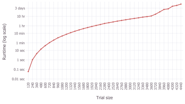
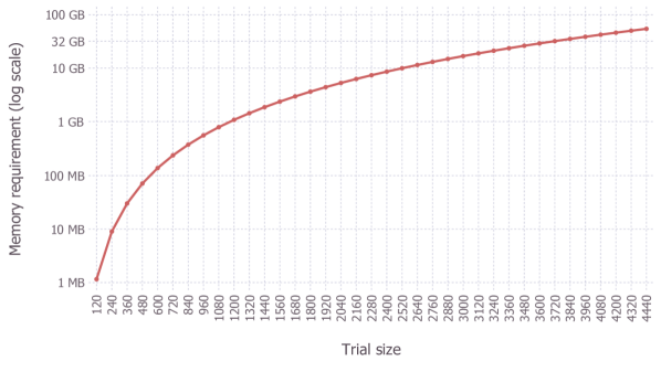
Figure 1: An illustration of computational complexity of online calculation of the deterministic Bayesian decision-theoretic design over a range of trial sizes.

For finding the best action for each state via this approach, the transition probabilities are Bayesian, and

• the conventional assumption is to take as information state $\boldsymbol{i}$ (that does not change over time) the prior distribution on each arm $k$;

• the action set is constant, $|\mathcal{A}|=3$;

Since Theorem 1 is true for any design, it is also true for the optimal design, which is derived using the Bellman equation, which is an optimization equivalent of the Poisson equation.

Theorem 2.

The two reward definitions give the same optimal design and to the same optimal expected total reward.

The conventional assumption is that the two pure actions are deterministic, i.e., $p_{C}^{1}=p_{D}^{2}=1,p_{C}^{2}=p_{D}^{1}=0$, which we will refer to as the deterministic Bayesian decision-theoretic design, despite the fact that randomization is allowed when both actions are optimal.

A more general setting, in which the pure actions are allowed to be randomized instead of deterministic, was proposed in Cheng and Berry, (2007) and further developed in Williamson et al., (2017). In fact, such a setting provides a continuum of designs, ranging from the deterministic Bayesian decision-theoretic design to the equal randomized allocation design, recovered by setting $p_{C}^{1}=p_{C}^{2}=p_{D}^{1}=p_{D}^{2}=1/2$.

5.2.1 Optimal — Dynamic Programming

The Bayesian decision-theoretic model can be solved by (stochastic) dynamic programming (DP), which comprises of a calculation starting by enumerating all the possible states in the final time period, continuing backwards in time while employing the Bellman equation in every state. Unfortunately, complete structure of the optimal design is unknown, thus numerical computation is the only way of obtaining it.

Figure 1 illustrates the computational complexity of online calculation (i.e., outputting the optimal action of the initial state) of this design, using a state-of-the-art package BinaryBandit in Julia programming language. In the number of elements (i.e., without multiplying by the memory required for each element), the memory requirement presented in Figure 1(right) is $2$ times larger than that of Gluss, (1962) because of his elimination of symmetric states, which can be done if the prior Beta distributions are the same for the two arms.

The computational complexity of offline calculation (i.e., outputting the optimal actions of all possible states) of this design is very similar to online calculation in terms of the runtime, but radically different in terms of memory requirement. Using the BinaryBandit Julia package, a computer with 32GB RAM is able to solve the problem of up to trial size $T=1,440$, keeping all the optimal actions in RAM during the calculations. For practical purposes, however, it may be possible to store parts of the solution on hard disk and thus relieve RAM memory to allow calculation for larger trial sizes.

A number of author’s colleagues and PhD students who had programmed this design for their needshave kindly provided runtimes of their code implementations, which are presented in Table 2 for comparison, indicating that the BinaryBandit package is two orders of magnitude faster than ad hoc codes and is able to solve a few times larger problems.

Software	RAM	$T=60$	$T=120$	$T=180$	$T=240$	$T=300$	$T^{\max}$
Julia 0.6.2 & ad hoc	12 GB	2sec	22sec	108sec	331sec	789sec	420
Julia 1.0.1 & ad hoc	12 GB	1sec	17sec	82sec	262sec	643sec	420
R & ad hoc	16 GB	1sec	12sec	59sec	191sec	N/A	240
Julia 1.0.1 & BB	31 GB	0.0036sec	0.046sec	0.23sec	0.73sec	1.6sec	1440
R & ad hoc	5 GB	1sec	6sec	26sec	84sec	209sec	420
Julia 1.0.1 & BB	31 GB	0.0040sec	0.056sec	0.27sec	0.91sec	2.8sec	4440

Table 2: A comparison of runtime of the Bayesian decision-theoretic design for $T=60:60:300$ and the largest horizon $T^{\max}$ (as a multiple of $60$) which does not give an out-of-memory error using code implementations by author’s colleagues and students. The top four are for offline calculation, the bottom two are for online calculation. BB refers to the use of the BinaryBandit package.

5.2.2 Asymptotically Optimal — Gittins and Whittle Index Rules

The structure of the optimal Bayesian decision-theoretic designs with deterministic pure actions is however known when considering the rewards over an infinite horizon $T\to+\infty$ and discounted with a geometrically-distributed discount factor $0<\gamma<1$. Gittins and Jones, (1974) discovered that optimal allocations can be characterized by an index rule, which allows (Gittins) index values to be calculated for every arm separately, and which at every time epoch allocates a subject to the arm with the highest Gittins index value (breaking the ties arbitrarily). See, e.g., Gittins, (1979, 1989); Gittins et al., (2011) for general theory on the Gittins index.

Although theoretically appealing and useful in many other problems, in the setting of the Bayesian decision-theoretic design it does not provide an ultimate solution, because the states are time-dependent and the horizon $T$ is finite. Still, the Gittins index rule can be used as an approximation to the optimal design, being asymptotically optimal as $T\to+\infty$. It decreases the computational complexity of the offline calculation notably because of a decreased size of the problem (one arm, i.e. two dimensions), but is still computed by dynamic programming, which is computationally demanding. In its calculation, however, it is necessary either to use a discount factor and/or a horizon truncation, or to compute it for every horizon $T$ considered by adding the remaining number of subject allocations as a third dimension. In the former case, the resulting index rule is only an approximation and tends to focus on learning less than the optimal design, see e.g. Villar et al., (2015). In the latter case, Niño-Mora, (2011, Section 6.2) provides a comparison of an approximate, so-called calibration, algorithm (using a grid of values to desired accuracy) and an exact algorithm for the calculation of the Whittle index values, showing that already $T\leq 100$ requires several GB of RAM, which suggests that the calibration algorithm with a grid of not more than $4$ significant digits is the only practical method for larger horizons.

Besides the requirement of infinite horizon, the theory of the Gittins index only applies when the pure actions are deterministic. When these are randomized, the problem becomes so-called restless, meaning that more than one arm can change its state in every period. Also, even when the pure actions are deterministic, but the horizon is finite, the problem can be seen as restless, by adding the remaining number of subject allocations to the state of each arm. Whittle, (1988) proposed to solve the restless problem also by an index rule, acknowledging that such a rule would not necessarily be optimal, but conjecturing that it would admit a form of asymptotic optimality as both the number of arms and the number of allocated arms in each period grow to infinity at a fixed proportion, which was eventually proved in Weber and Weiss, (1990) under some technical assumptions. Whittle defined an index, which reduces to the Gittins index in the non-restless setting, which became known as the Whittle index. The above discussion suggests that the Whittle index rule is conceptually more appropriate and more accurate than the Gittins index rule, and this was confirmed for the Bayesian decision-theoretic design numerically, see, e.g., Villar et al., (2015); Villar, (2018). The computational complexity of the approximate Whittle index values calculated by the calibration method for every horizon $T$ considered (using a grid of values to desired accuracy) is similar to that of the approximate Gittins index values using the same method.

Note that both the Gittins and Whittle index rule require to keep $3$ elements in the one-arm state, so the reduction from the optimal two-armed problem is only by one dimension. Moreover, in offline calculation, the index values that need to be stored are non-integer, thus require $64$ bits per one-arm state, while the offline calculation of the solution to the two-armed problem stores directly optimal actions, which require $2$ bits per two-arm state. Thus, the index rules (calculated to a few significant digits) are typically preferable to dynamic programming in calculation for horizons around $T\geq 1000$ and only if planned to be used for evaluation by simulation or for implementation in practice. However, Kaufmann, (2018) reports that she was able to compute the Gittins index values only up to $T=1000$.

Of course, advantages of index rules become important in problems with more than two arms, in which dynamic programming suffers from the curse of dimensionality. A discussion of such problems is however beyond the scope of this paper.

5.2.3 Approximately Optimal — Approximate Dynamic Programming

Several general approaches have been proposed to deal with the curse of dimensionality of stochastic optimization problems, which are collectively known as the approximate dynamic programming. There is a number of approximation techniques, but broadly focus on problem size reduction (e.g., the state space is approximated by a grid for which optimal actions are computed, and interpolated on non-included states) and/or on simplification of function computations (e.g. the value function is approximated by looking at decisions only a few periods ahead). See, e.g., Powell and Ryzhov, (2018, Section 6.6), Ahuja and Birge, (2019).

We will describe one approach, which leads to a Bayesian design known as the knowledge gradient (BKG). The fundamental idea to reduce the amount of information and computation required for a decision in a given state at a given time epoch is to assume that this decision is the last one, and in the next period we will identify the better arm which will whence be allocated to all the remaining subjects. Frazier et al., (2008, Section 7.2) showed that it is optimal for a search variant (i.e., maximizing the final-period expected reward) of the two-armed bandit problem with continuous responses. A specific variant of this approach for our setting was presented in Powell and Ryzhov, (2012, Section 4.7.1) and further studied and improved in Edwards et al., (2017).

Let us denote by $\mu_{k}(\widetilde{s}_{k}(t),\widetilde{f}_{k}(t))$, or briefly $\widetilde{\mu}_{k}$, the belief, i.e., the mean of the posterior Beta distribution of arm $k$ calculated using posterior observations (i.e., both the observations and prior pseudo-observations), i.e.,

$$\widetilde{\mu}_{k}:=\frac{\widetilde{s}_{k}(t)}{\widetilde{s}_{k}(t)+\widetilde{f}_{k}(t)}.$$ (7)

We will further denote the belief conditional on an additional (not necessarily binary) observation $\delta$, respectively, by

$$\widetilde{\mu}_{k}^{+\delta}:=\frac{\widetilde{s}_{k}(t)+\delta}{\widetilde{s}_{k}(t)+\widetilde{f}_{k}(t)+1}.$$ (8)

Under independent prior Beta distributions, the allocation at epoch $t$ by this design is to the arm $k$ with currently the largest value of the following score

$$\begin{cases}\widetilde{\mu}_{k}+(T-t-1)\widetilde{\mu}_{\ell}&\text{ if }\widetilde{\mu}_{\ell}\geq\widetilde{\mu}_{k}^{+1}\\ \widetilde{\mu}_{k}+(T-t-1)\left[(1-\widetilde{\mu}_{k})\widetilde{\mu}_{\ell}+\widetilde{\mu}_{k}\widetilde{\mu}_{k}^{+1}\right]&\text{ if }\widetilde{\mu}_{k}^{+1}\geq\widetilde{\mu}_{\ell}\geq\widetilde{\mu}_{k}^{+0}\\ \widetilde{\mu}_{k}+(T-t-1)\widetilde{\mu}_{k}^{+\widetilde{\mu}_{k}}&\text{ if }\widetilde{\mu}_{k}^{+0}\geq\widetilde{\mu}_{\ell}\end{cases}$$ (9)

where $\ell$ refers to the other arm, and ties are broken randomly. Although this score can be interpreted as capturing the allocation priority similarly to the Gittins and Whittle indices, it depends on the state of the other arm, thus, strictly speaking, it is not an index.

5.3 Naïve Designs

While in the previous subsection we described designs which are horizon-dependent and forward-looking in the way of making allocation decisions, we now turn our attention to horizon-independent designs and present a number of different naïve approaches in this subsection. Such designs are computationally simple and easy to interpret, hence sometimes more appealing for practical use. It turns out that such deterministic designs are either related to myopia ($T=1$) or to utopia ($T=+\infty$).

We will say that a design leads to complete learning, if in the problem considered over an infinite horizon (i.e., $T=+\infty$) it identifies the better arm almost surely. It is easy to see that to achieve complete learning it is necessary to allocate each arm infinitely often.

5.3.1 Myopic Index Rules

Bradt et al., (1956) considered the setting in which one knows the two-point set $\{\theta_{C},\theta_{D}\}$, but does not know which arm is which, and proved that if $\theta_{C}+\theta_{D}=1$, then it is optimal, under any prior distributions, to deterministically allocate every subject to the arm with currently largest Bayesian expected one-period reward. The also proved the same in the case $\theta_{C}+\theta_{D}=1$ when the set $\{\theta_{C},\theta_{D}\}$ is unknown. For the case $\theta_{C}+\theta_{D}\neq 1$ with known set $\{\theta_{C},\theta_{D}\}$ they proved that such a design leads to complete learning and conjectured that it is optimal in terms of the Bayesian expected number of successes. They also discussed that such a design is not optimal if both of these assumptions are dropped.

Note that under independent Beta prior distributions, the allocation at epoch $t$ by this design is to the arm $k$ with currently the largest mean calculated using posterior observations (i.e., both the observations and prior pseudo-observations), i.e.,

$$\frac{\widetilde{s}_{k}(t)}{\widetilde{s}_{k}(t)+\widetilde{f}_{k}(t)}$$ (10)

where ties are broken randomly. We call this the Bayesian myopic (BM) design, because it takes an action which is best for the next subject only and ignores the future.

Feldman, (1962) also considered the setting with known two-point set $\{\theta_{C},\theta_{D}\}$ and further generalized the optimality of the Bayesian myopic design. Berry, (1972, Section 8) realized that the setting with known two-point set $\{\theta_{C},\theta_{D}\}$ (i.e., with strong between-arm dependence) is equivalent to the two-armed problem with independent arms with two-point prior distributions. Kelley, (1974) further generalized the setting with dependent arms and identified conditions for optimality of the Bayesian myopic design.

We also consider the frequentist myopic (FM) design, which allocates each arm once in the first two periods, and then deterministically allocates every subject to the arm with currently the largest mean calculated using the observations only (breaking the ties randomly), i.e.,

$$\frac{s_{k}(t)}{s_{k}(t)+f_{k}(t)}$$ (11)

Such a design was mentioned in Bather, (1981, Eq. (1.1)) and called “play the favourite”. Note that BM and FM are equivalent if and only if $\widetilde{s}_{C}(0)=\widetilde{f}_{C}(0)=\widetilde{s}_{D}(0)=\widetilde{f}_{D}(0)=0$.

Berry, (1978, Section 3) established that, in the setting with known two-point set $\{\theta_{C},\theta_{D}\}$, in which the BM design is optimal, at any epoch $t$ at which the posterior probability that arm $C$ is better than arm $D$ is $1/2$, it is optimal to allocate to the arm with currently the greatest difference between the number of successes and the number of failures. Several tie-breaking rules can be used but they only affect the performance marginally, so these are not discussed here in detail. We refer to this as the Bayesian greatest difference first (BGDF) design. The Bayesian performance of this design was illustrated numerically to be near optimal (Berry,, 1978) and to outperform the BM design (Villar,, 2018). The mentioned condition applies when the one-arm prior distributions satisfy $\widetilde{s}_{C}(0)=\widetilde{f}_{C}(0)=\widetilde{s}_{D}(0)=\widetilde{f}_{D}(0)$, as in this paper, and note that in that case the frequentist analogue, FGDF, yields an equivalent design.

5.3.2 Utopic Index Rules

In the frequentist setting, Robbins, (1952) introduced the deterministic “stay-with-a-winner & switch-on-a-loser” design, in which the first allocation is made randomly, and then the same arm is allocated whenever the observed response is a success, while the other arm is allocated whenever the observed response is a failure. He realized that it leads to complete learning, but fails to achieve the maximum expected proportion of successes, because it allocates the worse arm at a regular rate.

Interestingly, many of the deterministic designs actually have the “stay-with-a-winner” property. It is easy to see that the BM, FM, BGDF and FGDF all have it. In the Bayesian setting, Berry, (1972, Theorem 6.2) proved the “stay-with-a-winner” property for the deterministic DP design. Formally, the “stay-with-a-winner” property in this approach is: if arm $k$ is optimal in period $t\leq T-2$, the subject is allocated to it and its response is a success, then arm $k$ is uniquely optimal in period $t+1$. Contrary to the above, the “switch-on-a-loser” property is not, in general, satisfied by these designs. When one arm looks significantly better than the other one, the designs would not switch after observing a failure on the former arm. See, e.g., Berry and Fristedt, (1985, p. 79).

Berry, (1972, Conjecture A, p. 892) conjectured that for a large number of remaining allocations (i.e. at epochs $t\ll T$), the only criterion for Bayesian optimality in the DP design is the difference between the posterior number of failures on the two arms. (He did not specify what to do if there is the same number of failures on the two arms.)

Kelly, (1981) studied the Gittins index rule in the infinite-horizon setting (in which it is optimal) as the discount factor approaches one (i.e. the undiscounted setting) and established, under a technical condition on the prior distributions, that the Gittins index rule reduces to the following rule which we call the frequenist least failures first (FLFF) design: at every time epoch, allocate the subject to the arm with least observed number of failures, breaking the ties in favor of any arm with greatest observed number of successes (breaking the double ties arbitrarily).

Although the similarity to Berry’s conjecture is remarkable, Kelly, (1981, Remark 4.15) stated that there seems to be no immediate link between these two statements, and that Berry’s conjecture may require a technical condition on the prior distributions. Kelly, (1981, Remark 4.7) further elucidated that FLFF is a slight variation of the “stay-with-a-winner & switch-on-a-loser” design in Robbins, (1952). Indeed, it is easy to see that FLFF has the “stay-with-a-winner” property. After observing a failure, it switches if the other arm has lower number of failures, but it stays or switches accordingly to the greater number of successes if the number of failures on both arms is the same.

Analogously, we call the Bayesian least failures first (BLFF) design the one based on posterior numbers of successes and failures rather than on the observed ones. If the prior distributions on the two arms are the same, then this design is equivalent to the FLFF design, but if they are not, then the arm with lower number of posterior failures will be allocated without switching (at least) until the number of failures on the two arms becomes the same.

We would like to highlight that the three radically different “schools” of the bandit problem, namely Robbins’, Berry’s and Gittins’, all led to the FLFF design with only slight variations. The “stay-with-a-winner & switch-on-a-loser” design may be useful in some practical situations because it only depends on the last observation, not on the numbers of successes and failures over the whole history.

5.4 Reinforcement Learning — UCB Index Rules

Lai and Robbins, (1985) laid out the theory of asymptotically optimal allocation and were the first to actually use the term “upper confidence bound” (UCB). They wrote it in quotes, as the quantity it refers to depends on time period $t$, and is thus not the conventional upper bound of confidence intervals, but can be interpreted as the upper confidence bound with significance level $1/t$. Lai, (1987, Eq. (2.6)) introduced a UCB index rule using the Kullback-Leiber divergence and Agrawal, (1995, Example 5.7) developed UCB index values which are inflations of the observed mean proportion of successes. The theory was further extended in Burnetas and Katehakis, (1996) to multivariate and non-parametric distributions. The first simple UCB index rules with finite-time theoretical guaranties were developed in Auer et al., (2002). See, e.g., Bubeck and Cesa-Bianchi, (2012); Kaufmann and Garivier, (2017); Lattimore and Szepesvári, (2019) for accounts of subsequent developments.

The use of the observed mean proportion of successes in defining an index rule is attractive mainly because it is the maximum likelihood estimator of the success probability in the static setting of the design of experiments. Index rules that use time-dependent inflations of the observed mean proportion of successes were proposed and investigated even before Lai and Robbins, (1985), e.g., Bather, (1980, 1981); Abdel Hamid, (1981) in frequentist setting and Gittins and Jones, (1974); Glazebrook, (1980); Gittins and Wang, (1992) in Bayesian setting.

Following Bubeck and Cesa-Bianchi, (2012, Section 2), we consider the popular $\alpha$UCB design which allocates each arm once in the first two periods, and then deterministically allocates every subject to the arm with currently the largest index (breaking ties randomly) of the form

$$\frac{s_{k}(t)}{s_{k}(t)+f_{k}(t)}+\sqrt{\frac{\alpha\cdot\ln(t+1)}{s_{k}(t)+f_{k}(t)}}$$ (12)

where $\alpha>0$. The original design introduced in Auer et al., (2002) used $\alpha=2$. Theoretical upper bounds currently exist for $\alpha>1$, but researchers have noticed empirically that lower values of $\alpha$ typically lead to better performance and some used $\alpha=1$, see, e.g., Cserna et al., (2017). In our numerical experiments (not reported here) we found that approximately the best performance is achieved with $\alpha=0.18$.

Many other types of UCB designs have been developed, see e.g., Kaufmann, (2018, Figure 2) for comparison of some of them. Besides designs based on idea of UCB, there is a number of popular designs with randomized actions, e.g., epsilon-greedy, Boltzmann exploration, Thompson sampling, etc.

5.5 Biostatistics

Blinding of patients and personnel to the allocated treatment is an important desideratum in many types of clinical trials to mitigate a variety of biases such as performance bias, detection bias and attrition bias (Higgins and Green,, 2011, Section 8.4). If allocation is deterministic, the patients and personnel can, if they know the state of the trial, identify the allocated treatment with certainty or high probability. Thus, some amount of randomness in the allocation decision is desirable. Moreover, the theory of design of experiments explains that randomization is important for mitigation of the selection bias, for ensuring similarity in the treatment groups and for providing a basis for inference, which are essential for making valid conclusions at the end of a trial (Rosenberger et al.,, 2019). Thus, in clinical trials theory and practice, a lot of attention is paid to designs with randomized actions (Rosenberger and Lachin,, 2015), although it should also be noted that not all types of clinical trials require or allow to implement blinding and randomization. There are three major approaches to adaptive randomization: (i) Bayesian Response-Adaptive Randomization, starting with Thompson, (1933), generalized in Thall and Wathen, (2007) (see also Berry et al., (2011, p. 156)), and recently studied also in the reinforcement learning literature (see, e.g., Agrawal and Goyal, (2012)); (ii) Frequentist Pólya Urn Randomization, which is a randomized version of the “stay-with-a-winner & switch-on-a-loser” design, starting with Wei and Durham, (1978); and (iii) Randomized Index Rules such as those proposed by Bather, (1980, 1981); Abdel Hamid, (1981) in frequentist setting and by Glazebrook, (1980) in Bayesian setting.

Note that the term “bandit” usually does not appear in the relevant biostatistics literature.

5.6 Combination Designs

Many researchers have suggested to use one design for the first $N$ subjects and use another one for the remaining $(T-N)$ subjects. This idea appeared implicitly in early papers on sequential design of experiments, considering the 1:1 design initially (on a sample of size $N$), and then sticking to the arm with higher mean (concluded at a given significance level) forever, since that approach assumes $T=+\infty$. Cheng et al., (2003) found that when $T$ is finite, for this combination design it is optimal for $N$ to be of the order of $\sqrt{T}$, and, in the particular case of prior Beta distribution with parameters $(1,1)$ on each arm, the optimal $N\to\sqrt{2T}$ asymptotically as $T\to+\infty$ (and is slightly lower for finite horizons).

Hoel et al., (1972) considered a setting in which $T$ is not fixed in advance, but the allocation is stopped if a predefined difference in the number of successes is reached. They proposed to start with the arm alternating design (i.e., a deterministic version of 1:1), and then to switch to the “stay-with-a-winner & switch-on-a-loser” design if the estimate of $\max\{\theta_{C},\theta_{D}\}$ is greater than $0.6$ and continue with arm alternating otherwise. This paper is just one example from the work in the area of ranking and selection.

Zelen, (1969, Section 4) proposed to initially use the “stay-with-a-winner & switch-on-a-loser” design, and then to stick to the arm with higher mean. He found that this is better than the classic combination if $\theta_{C}+\theta_{D}\geq 1$ and the value of $N\approx T/3$ yields a nearly-optimal number of successes.

Kelly, (1981, Remark 4.10) elucidated that the optimal Bayesian decision-theoretical design in the discounted setting can be regarded as having three stages: first, BLFF, which he refers to as “information gathering”, then it moves further and further away from that design, and finally it always allocates to the same arm. Villar, (2018, Section 3.4) provided some illustrative numerical evaluation of these stages for the Gittins and Whittle index rules.

Motivated by the above and by the discussion in subsubsection 5.3.2, in this paper we consider three combination designs in which the designs used are BLFF in the first stage, followed by BM, $\alpha$UCB and BMSF, respectively, and one combination rule in which the designs used are 1:1 in the first stage, followed by BMSF:

• BLFF+BM with $N=\sqrt{4T}$

• BLFF+$\alpha$UCB with $N=\sqrt{4T}$

• BLFF+BMSF with $N=\sqrt{9T}$

• 1:1+BMSF with $N=\sqrt{2T}$

The lengths of the first stage using BLFF have been obtained heuristically based only on a small numerical study and so they are not necessarily overall optimal, and surely not optimal for each particular scenario. To the best of our knowledge, these three designs have not been studied previously and their theoretical analysis is an open problem. Note that using BMSF in the second stage represents the situation in which the arm with higher mean (most successes is approximately equivalent to highest mean since BLFF keeps the number of failures balanced up to a difference of $1$) after the first stage is allocated to all the subjects in the second stage since only the allocated arm can collect additional successes. This is inspired by but not fully equivalent to the design studied by Zelen, (1969, Section 4), because BLFF is not fully equivalent to “stay-with-a-winner & switch-on-a-loser”.

Using BM in the second stage is similar to BMSF, but allows for additional learning during the second stage: the mean of the arm with higher mean at the end of the first stage may eventually decrease below the mean of the other arm, at which moment the allocation switches to that arm (there may be more than one such “correction”). The combination design that uses $\alpha$UCB in the second stage is included because it has interesting performance, to be discussed in Section 6.

Design 1:1+BMSF is inspired by Cheng et al., (2003), although using BMSF in the second stage is not fully equivalent to sticking to the arm with higher mean at the end of the first stage, because 1:1 may lead to unbalanced allocation due to sampling variability.

6 Designs Performance

For some of the response-adaptive designs, theoretical values of or bounds on their performance exist. However, these are either asymptotic as $T\to+\infty$, or up to an additive and/or multiplicative constants, which are often large or unknown. For small ($T\approx 1:10^{2}$) and moderate ($T\approx 10^{2}:10^{4}$) horizons, computational evaluation is the most appropriate to illustrate designs performance.

In this section we report computational experiments in which every design is evaluated by backward recursion, i.e. at full computational accuracy (of Float64, which is of the order of $10^{\log(T)-16}$). For fairness, we only include deterministic designs and 1:1 as a benchmark (i.e. we exclude the biostatistics ones).

To the best of our knowledge, such accurate evaluation has only been reported for small horizons in the existing literature. For moderate horizons, which are often the most relevant in practice, for instance in clinical trials, designs are usually evaluated by simulation, which is remarkably less accurate.

We present the performance in terms of both the proportion of successes and (equivalently) the regret number of successes, as these provide complementary insights. See Appendix C for small horizons, in which the performance of some of the designs is fundamentally different.

6.1 Bayesian Performance — Moderate Trial Sizes

Figure 2 illustrates the Bayesian performance of the Bayesian decision-theoretic design for $T=120:120:4440$. Although it is an interesting way of summarizing the performance, it has three major drawbacks: (i) it is a simple average over all the possible pairs of parameters $(\theta_{C},\theta_{D})$, while in practice one would be interested in a particular subset of the whole parameter space, possibly weighted in a particular way; (ii) it presents the Bayesian value in which the observations happen according to the belief at every time epoch rather than being fixed over the whole horizon, which blurs its interpretation because the beliefs are biased and which is less desirable since in practice one would be interested in the value under the true (unknown) success probabilities; (iii) it depends on the prior distributions, so a choice needs to be made or it needs to be computed for a number of different options.

Nevertheless, Figure 2 is instrumental in giving an idea about the order of magnitude of the objective, and in particular it is interesting to observe that the regret number of successes is increasing and concave, taking value of around $5$ for the trial size of $3000$ and, by extrapolation, it is likely to be below one per mille of the trial sizes beyond $10^{4}$.

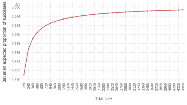
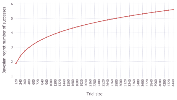
Figure 2: An illustration of two (equivalent) Bayesian performance measures evaluated for the deterministic Bayesian decision-theoretic design over a range of moderate trial sizes.

6.2 Frequentist Performance — Moderate Trial Sizes

In this subsection we evaluate and compare the frequentist performance of the above designs for for $T=120:60:1200\cup 1200:300:2400$. We do so in four scenarios: $(\theta_{C},\theta_{D})\in\{(0.1,0.3),(0.3,0.5),(0.5,0.7),(0.7,0.9)\}$. These scenarios are a natural choice, and have been previously considered, e.g., $(0.3,0.5)$ in Lai, (1987, Table 3), Brezzi and Lai, (2002, Table 2), Villar et al., (2015, Table 5) and Villar, (2018, Table 6), $(0.7,0.9)$ in Lai, (1987, Table 3), and all of them in Hoel et al., (1972). Although conclusions from a number scenarios do not guarantee their validity in other scenarios, we have found these four scenarios to be illustrative enough to provide negative conclusions for many designs.

We report both the proportion of successes, in Figure 3, and the regret number of successes, in Figure 4. Besides the mean, for each measure we report also the standard deviation, which can be considered as a secondary criterion providing additional insights into the performance of the designs.

1:1 is the worst design in terms of the mean and often the best in terms of the SD but, surprisingly, it is not always the best, meaning that in some scenarios there are designs that are better under both measures (all of these are combination designs, to be discussed below). BLFF notably improves the mean, increasingly so in the scenarios with higher success probabilities, while only marginally deteriorates the SD. They both over-explore.

The curves of BMSF, FM, BM, BGDF and BKG look approximately linear in both the mean and SD of the regret number of successes (approximately constant in both the mean and SD of the proportion of successes). The performance of BGDF and BKG is quite bad in general and heavily scenario dependent. BGDF’s mean deteriorates with more extreme success probabilities, but its SD improves with lower success probabilities. BKG’s mean and SD both improve with lower success probabilities, remarkably so in scenario $(0.1,0.3)$, in which the mean regret is the best of all designs and seems to be constant, while all the other designs’ mean regret is increasing.

There are three designs that perform particularly badly in all four scenarios: BMSF, FM and BM are dominated by almost all the other designs. High SD indicates that these three designs are extremely under-exploring: too aggressively sticking to one of the arms, and relatively often choosing the worse one. Among these three, BMSF is worse than the other two in both the mean and SD in all four scenarios. The performance order of FM and BM depends on scenario; BM’s mean remarkably improves with lower success probabilities, while FM’s mean improves with more extreme success probabilities. For these three designs it also holds that the better the mean, the better the SD, so in every scenario the order is identical under both measures.

The curves for the mean of all the remaining designs (DP, $\alpha$UCB, and the combination designs) look approximately concave, leading to significant improvement in the mean. Quantitatively, all three versions of $\alpha$UCB are almost identical across the four scenarios, indicating that its performance depends on the difference $\theta_{C}-\theta_{D}$ rather than on their respective values. Interestingly, the mean regret number of successes of 2UCB is more than $50\%$ higher than that of 1UCB, which is in turn around $3$ times higher than that of 0.18UCB, which is in turn still distinctively higher (between $20\%-100\%$, depending on scenario) than that of DP which is the best performing design except when dominated by BKG in scenario $(0.1,0.3)$. The mean regret of DP in scenario $(0.7,0.9)$ seems to be constant, while all the other designs’ mean regret is increasing. The SD of 2UCB and 1UCB is practically undistinguishable, while the SD of 0.18UCB is notably higher in the scenarios with higher success probabilities, with the SD of DP being in between.

The combination designs bring some surprising results. First, BLFF+2UCB is practically identical to 2UCB and BLFF+1UCB to 1UCB in all the scenarios and trial sizes, indicating that $\alpha$UCB initially behaves essentially as BLFF. That is however not true for BLFF+0.18UCB, which is similar but not identical to 0.18UCB: in terms of the mean being better in scenarios with higher success probabilities while being worse in those with lower success probabilities. The SD of BLFF+0.18UCB is always lower than that of 0.18UCB, and in particular it is the lowest of all designs except when dominated by 1:1 and BLFF in scenarios with low success probabilities.

Somewhat surprisingly, BLFF+BM performs quite well, roughly similarly to BLFF+0.18UCB in terms of the mean, although its SD is sometimes higher. BLFF+BMSF performs worse than BLFF+BM but still significantly better than 1UCB in terms of the mean, but its SD is notably higher. 1:1+BMSF is in most instances significantly worse than BLFF+BMSF both in terms of the mean and SD.

We summarize the above discussion as follows:

• DP may be the preferred design in terms of the mean in scenarios with high and moderate success probabilities;

• BKG may be the preferred design in terms of the mean in scenarios with low success probabilities;

• BLFF+0.18UCB may be the overall preferred design in terms of both the mean (higher weight) and the SD (lower weight);

• BLFF may be the overall preferred design in terms of both the mean (lower weight) and the SD (higher weight);

• 1:1 may be the preferred design in terms of the SD in scenarios with low and moderate success probabilities;

• BLFF+0.18UCB may be the preferred design in terms of the SD in scenarios with high success probabilities;

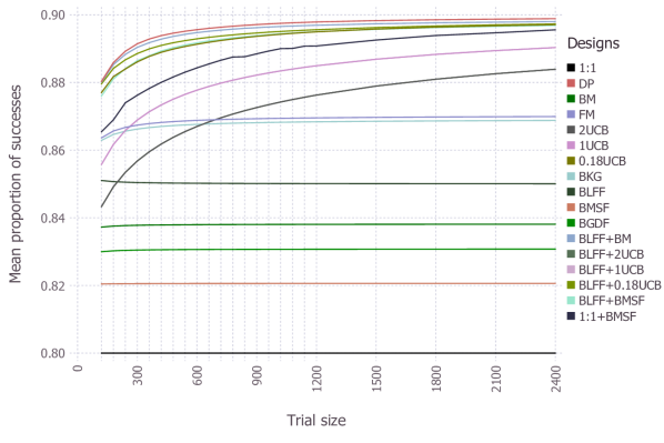
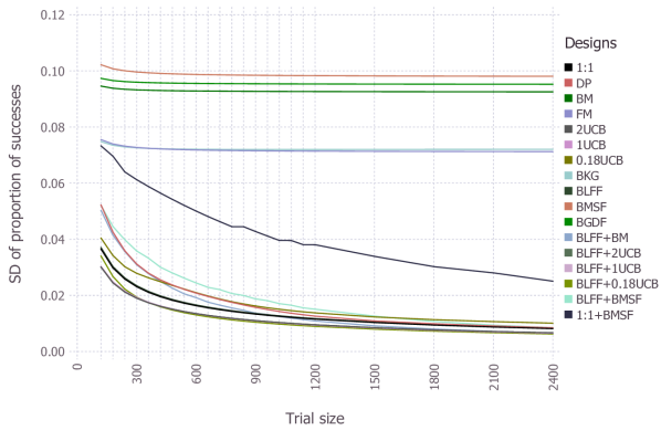
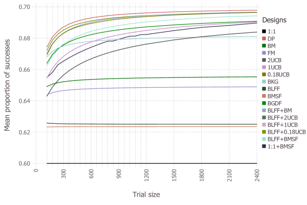
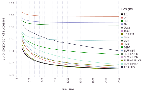
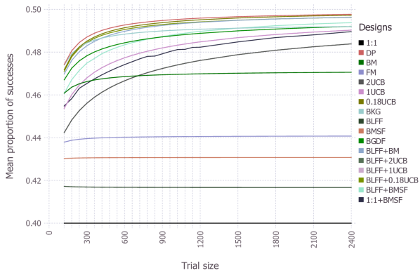
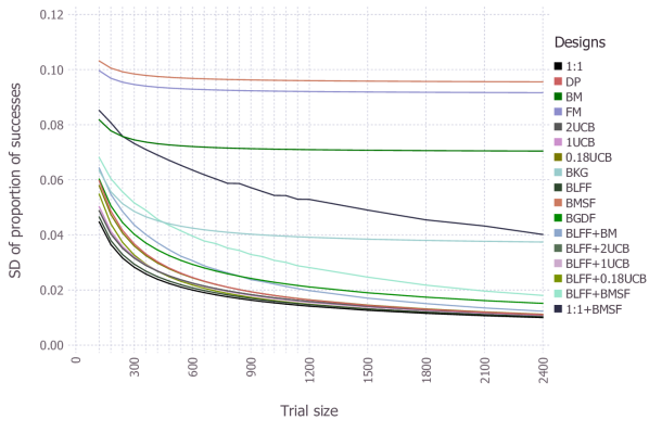
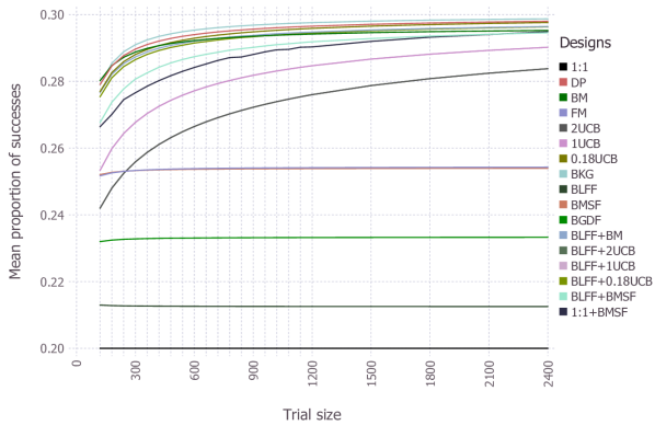
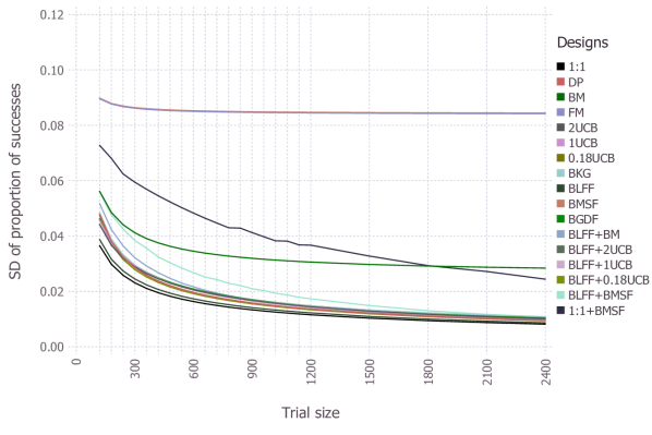
Figure 3: An illustration of performance (mean on the left, standard deviation on the right) in terms of the expected proportion of successes evaluated for deterministic designs over a range of moderate trial sizes, for $(\theta_{C},\theta_{D})=(0.7,0.9)$ in the first row, $(0.5,0.7)$ in the second row, $(0.3,0.5)$ in the third row, $(0.1,0.3)$ in the fourth row.

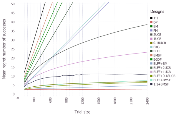
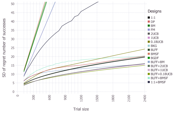
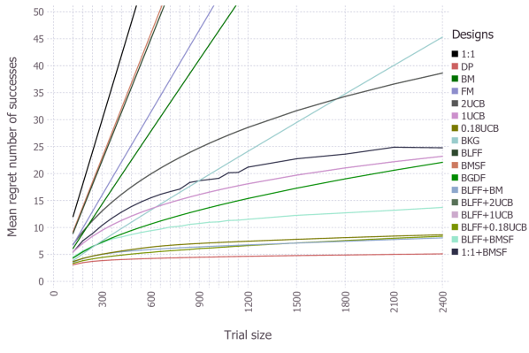
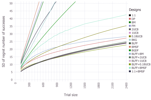
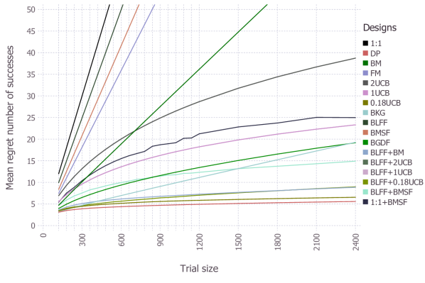
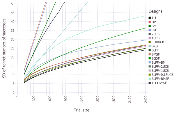
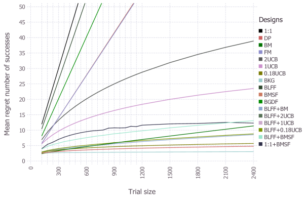
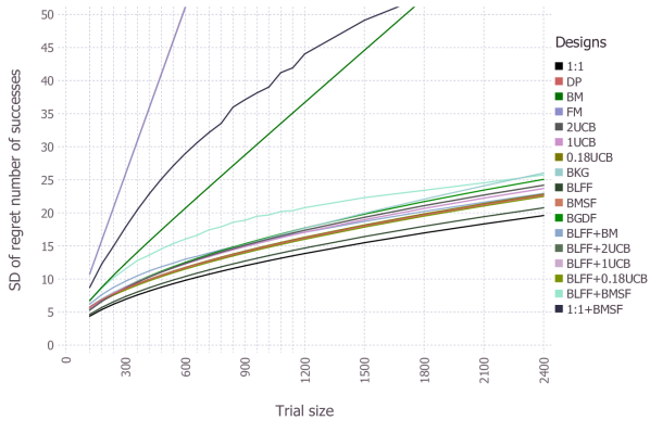
Figure 4: An illustration of performance (mean on the left, standard deviation on the right) in terms of the regret number of successes evaluated for deterministic designs over a range of moderate trial sizes, for $(\theta_{C},\theta_{D})=(0.7,0.9)$ in the first row, $(0.5,0.7)$ in the second row, $(0.3,0.5)$ in the third row, $(0.1,0.3)$ in the fourth row.

7 Myths

The hardness of the problem and the diversity of approaches mean that it is difficult for a single person to have complete information and full understanding of the many details. This paper is, to the best of our knowledge, first attempt to survey key ideas from multiple disciplines. Author’s engagement with researchers and practitioners from a number of fields has given him an impression of common beliefs that may not be fully correct, listed next.

7.1 Myth #1: The Bayesian Decision-Theoretic Design is Intractable

This myth seems to be widespread across disciplines, e.g., “The curse of dimensionality renders exact approaches impractical.” (Ahuja and Birge,, 2019); “Even in relatively benign setups the computation of the Bayesian optimal policy appears hopelessly intractable.” (Lattimore and Szepesvári,, 2019, Section 35.1); “Trials of a size up to 3500 patients would be feasible with today’s number #1 supercomputer (with 1.3 PB of RAM).” (Williamson et al.,, 2017).

Table 3 illustrates the evolution of what was reported as computationally tractable in the literature. Indeed, besides the two results in the 1960s that pre-date the era of personal computers, the existing literature gives an impression that solving the problem beyond $T=100$ is impractical or unfeasible. A closer look however reveals that no improvement seem to have been achieved since Berry, (1978) which appeared more than 40 years ago, despite the theoretical progress in computer science and technological progress in personal computers. In this paper we use a state-of-the-art package in Julia programming language written by the author, and show that on a standard laptop or desktop computer, the DP design can be computed for offline use or evaluated in online fashion in a few minutes ($T\approx 1,000$), in a few hours ($T\approx 2,000$), or in a few days ($T\approx 4,000$). 32GB of RAM allows storing (e.g. for offline use) of the whole design up to trial size around $1440$; when its storing is not needed (e.g. for Bayesian evaluation or for calculation of the initial action) it allows up to trial size around $4440$.

Publication	$T$	$T^{\max}$	SW, HW, RAM
Steck, (1964)	$25$	N/A	N/A, UNIVAC 1105, 54 kB
Yakowitz, (1969)	$5$	N/A	Fortran, N/A, N/A
Berry, (1978)	$100$	N/A	Basic (?), Atari (?), N/A
Ginebra and Clayton, (1999)	$150$	$180$	N/A, N/A, N/A
Hardwick et al., (2006)	$100$	$200$	N/A, N/A, N/A
Ahuja and Birge, (2016)	$96$	$240$	N/A, Mac 4GB
Williamson et al., (2017)	$100$	$215$	R, PC, 16GB
Villar, (2018)	$100$	N/A	Matlab, PC, N/A
Kaufmann, (2018)	$70$	N/A	N/A, N/A, N/A
This paper	$4440$	$4440$	Julia 1.0.1 & BB, PC, 32GB

Table 3: Horizons $T$ with reported results and $T^{\max}$ reported as the largest computationally tractable on a standard computer by backward recursion in the literature on two-armed problem with binary responses.

7.2 Myth #2: The Bayesian Decision-Theoretic Design is Optimal

The DP is Bayes-optimal, but that does not necessarily mean that it is optimal in the non-Bayesian objective, i.e. that it achieves the largest possible mean number of successes. Figure 4 and Figure 6 clearly show that other designs perform better in some scenarios.

7.3 Myth #3: The Gittins Index Rule Leads to Incomplete Learning

According to Brezzi and Lai, (2000): “…we give in Section 3 a simple proof of the incompleteness of optimal learning from endogenous data in the discounted multi-armed bandit problem… This generalizes Rothschild, (1974)’s result for Bernoulli two-armed bandits, and also the result of Banks and Sundaram, (1992) who show that there is positive probability of incomplete learning in multi-armed bandits with general distributions of rewards if the priors have finite support.” This is however true only in the discounted setting; Kelly, (1981) proved that the structure of the Gittins index rule in the undiscounted setting (see subsubsection 5.3.2) leads to complete learning.

7.4 Myth #4: The Gittins Index is Computationally Simpler than Dynamic Programming for the Two-Armed Problem

As we explain in subsubsection 5.2.2, there is a trade-off between accuracy and computational complexity of the Gittins index. For computing the Gittins index, all the algorithms use a truncation of the horizon, and due to numerical instability most of the numerical algorithms use a discount factor strictly lower than one although the appropriate one would be equal to one. So, there are three levels of approximation that the Gittins index requires, and such an approximate Gittins index rule may in the end not even perform better than the Myopic index rule (see e.g. Ahuja and Birge, (2016)).

7.5 Myth #5: The UCB Index Rule is Near-Optimal for the Finite-Horizon Problem

Section 6 illustrates that the 2UCB and 1UCB designs are significantly suboptimal, yielding five to tenfold mean regret number of successes than the optimal design. Tuning the coefficient even beyond the intervals required by theoretical analysis can significantly improve the performance, e.g. 0.18UCB yields around twofold mean regret number of successes than the optimal design, which is still too large to be considered near-optimal.

7.6 Myth #6: The Frequentist Mean Regret Number of Successes is Increasing

Lai and Robbins, (1985) presented a lower bound, valid under certain technical assumptions, indicating that the frequentist mean regret number of successes increases proportionally to $\log T$ as $T\to\infty$. Our computational results indicate that this is not necessarily true for all designs over finite horizons. For instance, the mean regret of DP in scenario $\theta_{C}=0.7,\theta_{D}=0.9$ (see Table 5) at $T=240$ is lower than that at $T=300$, and it is non-increasing over $T=660:60:1200$.

8 Conclusion

The aim of this paper to provide a unified account of approaches from various disciplines to the two-armed bandit problem. We have proposed problem terminology that we believe should not create conflicts with other existing terminology in most of the disciplines, to facilitate mutual learning. We have proposed to use backward recursion instead of simulation for more accurate evaluation. We have created a computational comparison of designs from different disciplines in a standardized set of scenarios. The computational results have showed that some of the simple ones (e.g. BLFF+BM and BLFF+BMSF) perform surprisingly well in our scenarios and outperform may of the more sophisticated and more studied ones. We have also showed that DP is tractable for much larger horizons than it is commonly believed. This suggests that there is a case for these to be used among benchmark designs when developing new designs.

We have given an account of approaches to the problem with the objective of maximizing the mean number of successes, which is linear across arms and over time. Most of the above designs, especially those horizon-ignorant, crucially depend on that property, and it is not clear how they could be modified if the objective changed to another one. The only exception is the DP and its variants, which are quite flexible to accommodate other finite-horizon objectives.

A significant area of research left out of this paper deals with practicalities of implementation of the designs, especially in the context of clinical trials, in which (i) the objective is different, because it focusses much more on estimation of the success probabilities, and (ii) there are additional constraints, e.g. requirement of a certain degree of randomization. A fair comparison of such designs would actually require a series of comparisons fixing the randomization degree and including only those designs that satisfy it. Such work is extensive and is left for a separate paper.

Appendix A Choosing the Prior Beta Distribution Parameters

While in the paper we have used the conventional Bayes parameters $\left(\widetilde{s}(0),\widetilde{f}(0)\right)=(1,1)$ for the prior Beta distribution of each arm, the trials in practice are often designed based on pilot trials, expert opinion, or real-world evidence, which can be summarized by the mean and the variance of the estimate of the success probability.

For Beta distribution with parameters $\widetilde{s}>0,\widetilde{f}>0$, the mean and the variance are

$$\mu(\widetilde{s},\widetilde{f}) =\frac{\widetilde{s}}{\widetilde{s}+\widetilde{f}}, \sigma^{2}(\widetilde{s},\widetilde{f}) =\frac{\mu(\widetilde{s},\widetilde{f})(1-\mu(\widetilde{s},\widetilde{f}))}{\widetilde{s}+\widetilde{f}+1}.$$ (13)

From these expressions we can obtain that for given mean $\mu$ and variance $\sigma^{2}$, the parameters of the Beta distribution are

$$\widetilde{s}(\mu,\sigma^{2}) =\mu\left[\frac{\mu(1-\mu)}{\sigma^{2}}-1\right], \widetilde{f}(\mu,\sigma^{2}) =(1-\mu)\left[\frac{\mu(1-\mu)}{\sigma^{2}}-1\right].$$ (14)

If parameters are $\widetilde{s}=0,\widetilde{f}>0$, the distribution is degenerate and the mean and the variance are

$$\mu(\widetilde{s},\widetilde{f}) =0, \sigma^{2}(\widetilde{s},\widetilde{f}) =0.$$ (15)

These are the only Beta distributions with mean equal to $0$. Such mean thus requires variance equal to $0$, and parameter $\widetilde{s}=0$ while $\widetilde{f}$ cannot be uniquely determined.

If parameters are $\widetilde{s}>0,\widetilde{f}=0$, the distribution is degenerate and the mean and the variance are

$$\mu(\widetilde{s},\widetilde{f}) =1, \sigma^{2}(\widetilde{s},\widetilde{f}) =0.$$ (16)

These are the only Beta distributions with mean equal to $1$. Such mean thus requires variance equal to $0$, and parameter $\widetilde{f}=0$ while $\widetilde{s}$ cannot be uniquely determined.

If parameters are $\widetilde{s}=0,\widetilde{f}=0$, the distribution is a symmetric two-point Bernoulli distribution with support $\{0,1\}$, and the mean and the variance are

$$\mu(\widetilde{s},\widetilde{f}) =\frac{1}{2}, \sigma^{2}(\widetilde{s},\widetilde{f}) =\frac{1}{4}.$$ (17)

This is the only Beta distribution with the largest possible variance, $1/4$. Such variance thus requires mean equal to $1/2$, and parameters are $\widetilde{f}=0,\widetilde{s}=0$.

	0.05	0.10	0.15	0.20	0.25	0.30	0.35	0.40	0.45	0.50
1/140	(0.28, 5.37)	(1.16, 10.44)	(2.53, 14.32)	(4.28, 17.12)	(6.31, 18.94)	(8.52, 19.88)	(10.80, 20.05)	(13.04, 19.56)	(15.14, 18.51)	(17.00, 17.00)
1/136	(0.27, 5.19)	(1.12, 10.12)	(2.45, 13.89)	(4.15, 16.61)	(6.12, 18.38)	(8.27, 19.29)	(10.48, 19.46)	(12.66, 18.98)	(14.70, 17.96)	(16.50, 16.50)
1/132	(0.26, 5.01)	(1.09, 9.79)	(2.37, 13.46)	(4.02, 16.10)	(5.94, 17.81)	(8.02, 18.70)	(10.16, 18.87)	(12.27, 18.41)	(14.25, 17.42)	(16.00, 16.00)
1/128	(0.25, 4.83)	(1.05, 9.47)	(2.30, 13.02)	(3.90, 15.58)	(5.75, 17.25)	(7.76, 18.12)	(9.84, 18.28)	(11.89, 17.83)	(13.81, 16.87)	(15.50, 15.50)
1/124	(0.24, 4.65)	(1.02, 9.14)	(2.22, 12.59)	(3.77, 15.07)	(5.56, 16.69)	(7.51, 17.53)	(9.52, 17.69)	(11.50, 17.26)	(13.36, 16.33)	(15.00, 15.00)
1/120	(0.24, 4.46)	(0.98, 8.82)	(2.14, 12.16)	(3.64, 14.56)	(5.38, 16.12)	(7.26, 16.94)	(9.20, 17.10)	(11.12, 16.68)	(12.92, 15.79)	(14.50, 14.50)
1/116	(0.23, 4.28)	(0.94, 8.50)	(2.07, 11.72)	(3.51, 14.05)	(5.19, 15.56)	(7.01, 16.35)	(8.89, 16.50)	(10.74, 16.10)	(12.47, 15.24)	(14.00, 14.00)
1/112	(0.22, 4.10)	(0.91, 8.17)	(1.99, 11.29)	(3.38, 13.54)	(5.00, 15.00)	(6.76, 15.76)	(8.57, 15.91)	(10.35, 15.53)	(12.02, 14.70)	(13.50, 13.50)
1/108	(0.21, 3.92)	(0.87, 7.85)	(1.92, 10.85)	(3.26, 13.02)	(4.81, 14.44)	(6.50, 15.18)	(8.25, 15.32)	(9.97, 14.95)	(11.58, 14.15)	(13.00, 13.00)
1/104	(0.20, 3.74)	(0.84, 7.52)	(1.84, 10.42)	(3.13, 12.51)	(4.62, 13.88)	(6.25, 14.59)	(7.93, 14.73)	(9.58, 14.38)	(11.13, 13.61)	(12.50, 12.50)
1/100	(0.19, 3.56)	(0.80, 7.20)	(1.76, 9.99)	(3.00, 12.00)	(4.44, 13.31)	(6.00, 14.00)	(7.61, 14.14)	(9.20, 13.80)	(10.69, 13.06)	(12.00, 12.00)
1/96	(0.18, 3.38)	(0.76, 6.88)	(1.69, 9.55)	(2.87, 11.49)	(4.25, 12.75)	(5.75, 13.41)	(7.29, 13.55)	(8.82, 13.22)	(10.24, 12.52)	(11.50, 11.50)
1/92	(0.17, 3.20)	(0.73, 6.55)	(1.61, 9.12)	(2.74, 10.98)	(4.06, 12.19)	(5.50, 12.82)	(6.98, 12.95)	(8.43, 12.65)	(9.80, 11.97)	(11.00, 11.00)
1/88	(0.16, 3.02)	(0.69, 6.23)	(1.53, 8.69)	(2.62, 10.46)	(3.88, 11.62)	(5.24, 12.24)	(6.66, 12.36)	(8.05, 12.07)	(9.35, 11.43)	(10.50, 10.50)
1/84	(0.15, 2.84)	(0.66, 5.90)	(1.46, 8.25)	(2.49, 9.95)	(3.69, 11.06)	(4.99, 11.65)	(6.34, 11.77)	(7.66, 11.50)	(8.91, 10.88)	(10.00, 10.00)
1/80	(0.14, 2.66)	(0.62, 5.58)	(1.38, 7.82)	(2.36, 9.44)	(3.50, 10.50)	(4.74, 11.06)	(6.02, 11.18)	(7.28, 10.92)	(8.46, 10.34)	(9.50, 9.50)
1/76	(0.13, 2.48)	(0.58, 5.26)	(1.30, 7.39)	(2.23, 8.93)	(3.31, 9.94)	(4.49, 10.47)	(5.70, 10.59)	(6.90, 10.34)	(8.01, 9.80)	(9.00, 9.00)
1/72	(0.12, 2.30)	(0.55, 4.93)	(1.23, 6.95)	(2.10, 8.42)	(3.12, 9.38)	(4.24, 9.88)	(5.38, 10.00)	(6.51, 9.77)	(7.57, 9.25)	(8.50, 8.50)
1/68	(0.11, 2.12)	(0.51, 4.61)	(1.15, 6.52)	(1.98, 7.90)	(2.94, 8.81)	(3.98, 9.30)	(5.06, 9.41)	(6.13, 9.19)	(7.12, 8.71)	(8.00, 8.00)
1/64	(0.10, 1.94)	(0.48, 4.28)	(1.07, 6.09)	(1.85, 7.39)	(2.75, 8.25)	(3.73, 8.71)	(4.75, 8.81)	(5.74, 8.62)	(6.68, 8.16)	(7.50, 7.50)
1/60	(0.09, 1.76)	(0.44, 3.96)	(1.00, 5.65)	(1.72, 6.88)	(2.56, 7.69)	(3.48, 8.12)	(4.43, 8.22)	(5.36, 8.04)	(6.23, 7.62)	(7.00, 7.00)
1/56	(0.08, 1.58)	(0.40, 3.64)	(0.92, 5.22)	(1.59, 6.37)	(2.38, 7.12)	(3.23, 7.53)	(4.11, 7.63)	(4.98, 7.46)	(5.79, 7.07)	(6.50, 6.50)
1/52	(0.07, 1.40)	(0.37, 3.31)	(0.84, 4.79)	(1.46, 5.86)	(2.19, 6.56)	(2.98, 6.94)	(3.79, 7.04)	(4.59, 6.89)	(5.34, 6.53)	(6.00, 6.00)
1/48	(0.06, 1.22)	(0.33, 2.99)	(0.77, 4.35)	(1.34, 5.34)	(2.00, 6.00)	(2.72, 6.36)	(3.47, 6.45)	(4.21, 6.31)	(4.90, 5.98)	(5.50, 5.50)
1/44	(0.05, 1.04)	(0.30, 2.66)	(0.69, 3.92)	(1.21, 4.83)	(1.81, 5.44)	(2.47, 5.77)	(3.15, 5.86)	(3.82, 5.74)	(4.45, 5.44)	(5.00, 5.00)
1/40	(0.04, 0.85)	(0.26, 2.34)	(0.61, 3.48)	(1.08, 4.32)	(1.62, 4.88)	(2.22, 5.18)	(2.83, 5.26)	(3.44, 5.16)	(4.00, 4.90)	(4.50, 4.50)
1/36	(0.04, 0.67)	(0.22, 2.02)	(0.54, 3.05)	(0.95, 3.81)	(1.44, 4.31)	(1.97, 4.59)	(2.52, 4.67)	(3.06, 4.58)	(3.56, 4.35)	(4.00, 4.00)
1/32	(0.03, 0.49)	(0.19, 1.69)	(0.46, 2.62)	(0.82, 3.30)	(1.25, 3.75)	(1.72, 4.00)	(2.20, 4.08)	(2.67, 4.01)	(3.11, 3.81)	(3.50, 3.50)
1/28	(0.02, 0.31)	(0.15, 1.37)	(0.39, 2.18)	(0.70, 2.78)	(1.06, 3.19)	(1.46, 3.42)	(1.88, 3.49)	(2.29, 3.43)	(2.67, 3.26)	(3.00, 3.00)
1/24	(0.01, 0.13)	(0.12, 1.04)	(0.31, 1.75)	(0.57, 2.27)	(0.88, 2.62)	(1.21, 2.83)	(1.56, 2.90)	(1.90, 2.86)	(2.22, 2.72)	(2.50, 2.50)
1/20	N/A	(0.08, 0.72)	(0.23, 1.32)	(0.44, 1.76)	(0.69, 2.06)	(0.96, 2.24)	(1.24, 2.31)	(1.52, 2.28)	(1.78, 2.17)	(2.00, 2.00)
1/16	N/A	(0.04, 0.40)	(0.16, 0.88)	(0.31, 1.25)	(0.50, 1.50)	(0.71, 1.65)	(0.92, 1.72)	(1.14, 1.70)	(1.33, 1.63)	(1.50, 1.50)
1/12	N/A	(0.01, 0.07)	(0.08, 0.45)	(0.18, 0.74)	(0.31, 0.94)	(0.46, 1.06)	(0.61, 1.12)	(0.75, 1.13)	(0.89, 1.08)	(1.00, 1.00)
1/8	N/A	N/A	(0.00, 0.02)	(0.06, 0.22)	(0.12, 0.38)	(0.20, 0.48)	(0.29, 0.53)	(0.37, 0.55)	(0.44, 0.54)	(0.50, 0.50)
1/4	N/A	N/A	N/A	N/A	N/A	N/A	N/A	N/A	N/A	(0.00, 0.00)

Table 4: Parameters $(\widetilde{s},\widetilde{f})$, rounded to two decimal places, of the Beta distribution that achieve the indicated values of mean (columns) and variance (rows). For mean greater than $0.5$, one can use the property of the Beta distribution that swapping the parameters gives the complementary mean.

Table 4 illustrates values of the parameters of the Beta distribution that correspond to particular pairs of mean and variance. Three well-known priors are highlighted in bold: the Bayes prior $\left(\widetilde{s},\widetilde{f}\right)=(1,1)$ with variance $1/12$, the Jeffreys prior $\left(\widetilde{s},\widetilde{f}\right)=(1/2,1/2)$ with variance $1/8$, and the Haldane prior $\left(\widetilde{s},\widetilde{f}\right)=(0,0)$ with variance $1/4$. All three are considered non-informative, although it may be argued that they provide different amount of information, e.g. the Bayes prior provides information that it is possible to observe each response, while the Haldane prior includes the setting that only one of the responses is possible.

Appendix B Equivalence of Reward Definitions

Throughout this section, we assume that information state $\boldsymbol{i}$ is constant and drop the explicit dependence on it. A particular design prescribes $a_{\boldsymbol{x}}\in\mathcal{A}:=\{1,2,3\}$ for every state $\boldsymbol{x}=(s_{C},f_{C},s_{D},f_{D})$. We first consider that the design is fixed.

Using the classic reward definition, the Poisson equation (cf. Makowski and Shwartz,, 2002) is: for all states satisfying $s_{C}+f_{C}+s_{D}+f_{D}=T$,

$$F_{T}(s_{C},f_{C},s_{D},f_{D})=0$$ (18)

and for all $t\in\mathcal{T}$ and for all states satisfying $s_{C}+f_{C}+s_{D}+f_{D}=t$,

$$F_{t}(s_{C},f_{C},s_{D},f_{D})=p_{C}^{a_{(s_{C},f_{C},s_{D},f_{D})}}\left[q_{C,(s_{C},f_{C},s_{D},f_{D}),1}\left(1+F_{t+1}(s_{C}+1,f_{C},s_{D},f_{D})\right)\right.$$

$$\left.+q_{C,(s_{C},f_{C},s_{D},f_{D}),0}\left(F_{t+1}(s_{C},f_{C}+1,s_{D},f_{D})\right)\right]$$

$$+p_{D}^{a_{(s_{C},f_{C},s_{D},f_{D})}}\left[q_{D,(s_{C},f_{C},s_{D},f_{D}),1}\left(1+F_{t+1}(s_{C},f_{C},s_{D}+1,f_{D})\right)\right.$$

$$\left.+q_{D,(s_{C},f_{C},s_{D},f_{D}),0}\left(F_{t+1}(s_{C},f_{C},s_{D},f_{D}+1)\right)\right]$$ (19)

Using the new reward definition, the Poisson equation is: for all states satisfying $s_{C}+f_{C}+s_{D}+f_{D}=T$,

$$G_{T}(s_{C},f_{C},s_{D},f_{D})=s_{C}+s_{D}$$ (20)

and for all $t\in\mathcal{T}$ and for all states satisfying $s_{C}+f_{C}+s_{D}+f_{D}=t$,

$$G_{t}(s_{C},f_{C},s_{D},f_{D})=p_{C}^{a_{(s_{C},f_{C},s_{D},f_{D})}}\left[q_{C,(s_{C},f_{C},s_{D},f_{D}),1}\left(G_{t+1}(s_{C}+1,f_{C},s_{D},f_{D})\right)\right.$$

$$\left.+q_{C,(s_{C},f_{C},s_{D},f_{D}),0}\left(G_{t+1}(s_{C},f_{C}+1,s_{D},f_{D})\right)\right]$$

$$+p_{D}^{a_{(s_{C},f_{C},s_{D},f_{D})}}\left[q_{D,(s_{C},f_{C},s_{D},f_{D}),1}\left(G_{t+1}(s_{C},f_{C},s_{D}+1,f_{D})\right)\right.$$

$$\left.+q_{D,(s_{C},f_{C},s_{D},f_{D}),0}\left(G_{t+1}(s_{C},f_{C},s_{D},f_{D}+1)\right)\right]$$ (21)

Lemma 1.

The recursion (20)–(21) evaluates the design equivalently to the recursion (18)–(19), and in particular, $G_{0}(0,0,0,0)=F_{0}(0,0,0,0)$.

Proof.

We will prove a more general result that for all $t\in\mathcal{T}\cup\{T\}$ and for all states satisfying $s_{C}+f_{C}+s_{D}+f_{D}=t$,

$$G_{t}(s_{C},f_{C},s_{D},f_{D})=F_{t}(s_{C},f_{C},s_{D},f_{D})+s_{C}+s_{D}.$$ (22)

From (18) and (20) it is clear that and for all states satisfying $s_{C}+f_{C}+s_{D}+f_{D}=T$,

$$G_{T}(s_{C},f_{C},s_{D},f_{D})=F_{T}(s_{C},f_{C},s_{D},f_{D})+s_{C}+s_{D}.$$ (23)

It remains to prove that for all $t\in\mathcal{T}$ and for all states satisfying $s_{C}+f_{C}+s_{D}+f_{D}=t$,

$$G_{t}(s_{C},f_{C},s_{D},f_{D})=F_{t}(s_{C},f_{C},s_{D},f_{D})+s_{C}+s_{D}$$ (24)

Using induction assumption for $t+1$

$$G_{t+1}(s_{C},f_{C},s_{D},f_{D})=F_{t+1}(s_{C},f_{C},s_{D},f_{D})+s_{C}+s_{D}$$ (25)

and plugging it into (21), we have

$$G_{t}(s_{C},f_{C},s_{D},f_{D})=p_{C}^{a_{(s_{C},f_{C},s_{D},f_{D})}}\left[q_{C,(s_{C},f_{C},s_{D},f_{D}),1}\left(F_{t+1}(s_{C}+1,f_{C},s_{D},f_{D})+s_{C}+s_{D}+1\right)\right.$$

$$\left.+q_{C,(s_{C},f_{C},s_{D},f_{D}),0}\left(F_{t+1}(s_{C},f_{C}+1,s_{D},f_{D})+s_{C}+s_{D}\right)\right]$$

$$+p_{D}^{a_{(s_{C},f_{C},s_{D},f_{D})}}\left[q_{D,(s_{C},f_{C},s_{D},f_{D}),1}\left(F_{t+1}(s_{C},f_{C},s_{D}+1,f_{D})+s_{C}+s_{D}+1\right)\right.$$

$$\left.+q_{D,(s_{C},f_{C},s_{D},f_{D}),0}\left(F_{t+1}(s_{C},f_{C},s_{D},f_{D}+1)+s_{C}+s_{D}\right)\right]$$

which after repetitively using (19) yields

$$G_{t}(s_{C},f_{C},s_{D},f_{D})=F_{t}(s_{C},f_{C},s_{D},f_{D})+p_{C}^{a_{(s_{C},f_{C},s_{D},f_{D})}}\left[q_{C,(s_{C},f_{C},s_{D},f_{D}),1}\left(s_{C}+s_{D}\right)\right.$$

$$\left.+q_{C,(s_{C},f_{C},s_{D},f_{D}),0}\left(s_{C}+s_{D}\right)\right]$$

$$+p_{D}^{a_{(s_{C},f_{C},s_{D},f_{D})}}\left[q_{D,(s_{C},f_{C},s_{D},f_{D}),1}\left(s_{C}+s_{D}\right)\right.$$

$$\left.+q_{D,(s_{C},f_{C},s_{D},f_{D}),0}\left(s_{C}+s_{D}\right)\right]$$

which gives $G_{t}(s_{C},f_{C},s_{D},f_{D})=F_{t}(s_{C},f_{C},s_{D},f_{D})+s_{C}+s_{D}$ because $\sum_{o}q_{k,(\boldsymbol{x},\boldsymbol{i}),o}=1$ for all $k$ and $\sum_{k}p_{k}^{a}=1$ for all $a$. ∎

Note that these two theorems do not hold in the model with (non-uniform) geometric discounting of future rewards, because there the order of observations matters.

Appendix C Designs Performance — Small Trial Sizes

Figure 5 and Figure 6 present the performance results for small trial sizes, analogously to Figure 3 and Figure 4, respectively.

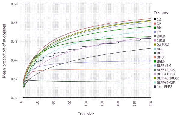
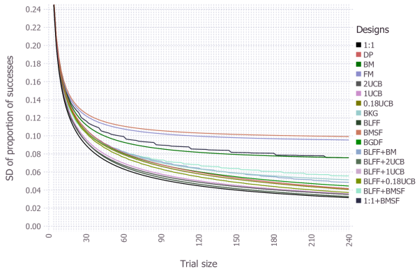
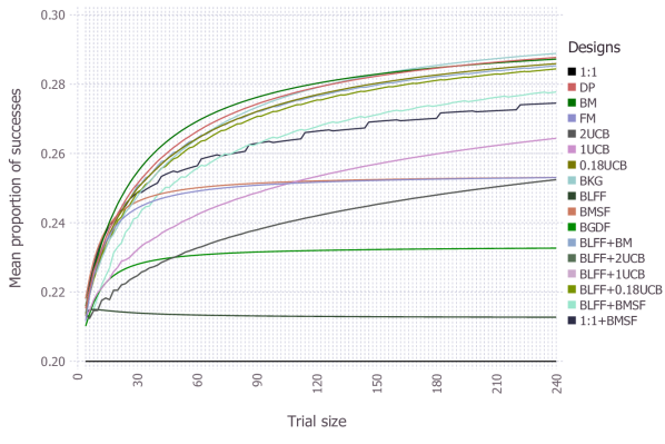
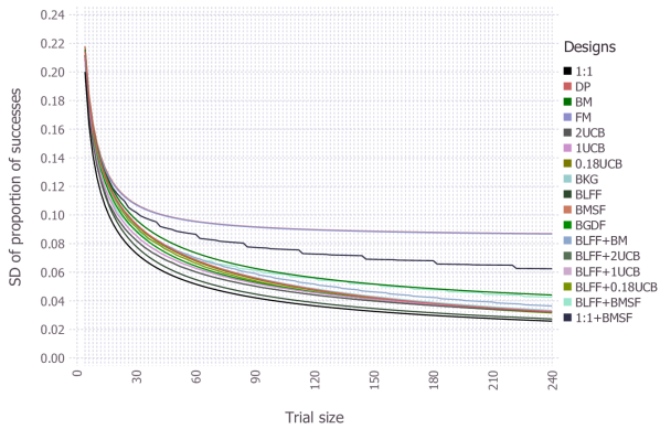
Figure 5: An illustration of performance (mean on the left, standard deviation on the right) in terms of the expected proportion of successes evaluated for deterministic designs over a range of small trial sizes, for $(\theta_{C},\theta_{D})=(0.7,0.9)$ in the first row, $(0.5,0.7)$ in the second row, $(0.3,0.5)$ in the third row, $(0.1,0.3)$ in the fourth row.

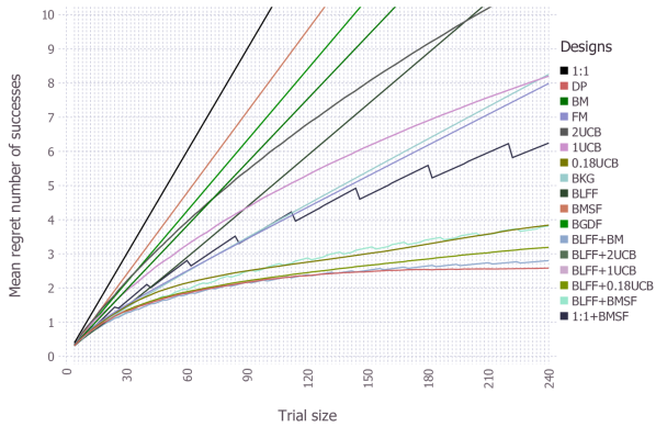
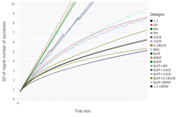
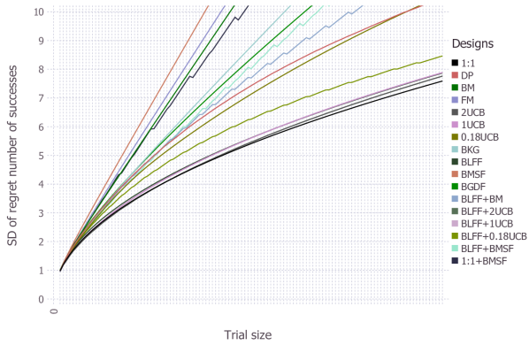
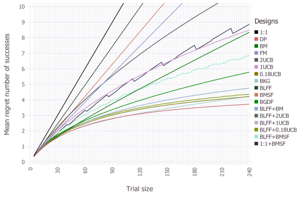
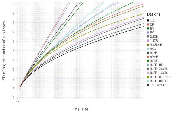
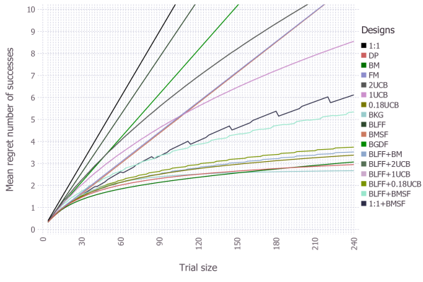
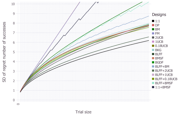
Figure 6: An illustration of performance (mean on the left, standard deviation on the right) in terms of the proportion of successes evaluated for deterministic designs over a range of small trial sizes, for $(\theta_{C},\theta_{D})=(0.7,0.9)$ in the first row, $(0.5,0.7)$ in the second row, $(0.3,0.5)$ in the third row, $(0.1,0.3)$ in the fourth row.

Appendix D Designs Performance — Tables

In Table 5, Table 6, Table 7, Table 8 we present values of the mean regret number of successes (rounded to $3$ significant digits) for trial sizes $60:60:1200$, which is a subset of those presented in the figures in Section 6 and Appendix C. In bold font are all the values which are equal or better than that of DP for each trial size. We further highlight with dark grey background (light grey background) the values that are lower than or equal to $10\%$ (greater than $10\%$ and lower than or equal to $20\%$) of the difference between DP and 2UCB.

Design $\backslash$ Trial size	60	120	180	240	300	360	420	480	540	600	660	720	780	840	900	960	1020	1080	1140	1200
1:1
DP
BM
FM
2UCB
1UCB
0.18UCB
BKG
BLFF
BMSF
BGDF
BLFF+BM
BLFF+2UCB
BLFF+1UCB
BLFF+0.18UCB
BLFF+BMSF
1:1+BMSF

Table 5: The mean regret number of successes under success probabilities 0.7 and 0.9.

Design $\backslash$ Trial size	60	120	180	240	300	360	420	480	540	600	660	720	780	840	900	960	1020	1080	1140	1200
1:1
DP
BM
FM
2UCB
1UCB
0.18UCB
BKG
BLFF
BMSF
BGDF
BLFF+BM
BLFF+2UCB
BLFF+1UCB
BLFF+0.18UCB
BLFF+BMSF
1:1+BMSF

Table 6: The mean regret number of successes under success probabilities 0.5 and 0.7.

Design $\backslash$ Trial size	60	120	180	240	300	360	420	480	540	600	660	720	780	840	900	960	1020	1080	1140	1200
1:1
DP
BM
FM
2UCB
1UCB
0.18UCB
BKG
BLFF
BMSF
BGDF
BLFF+BM
BLFF+2UCB
BLFF+1UCB
BLFF+0.18UCB
BLFF+BMSF
1:1+BMSF

Table 7: The mean regret number of successes under success probabilities 0.3 and 0.5.

Design $\backslash$ Trial size	60	120	180	240	300	360	420	480	540	600	660	720	780	840	900	960	1020	1080	1140	1200
1:1
DP
BM
FM
2UCB
1UCB
0.18UCB
BKG
BLFF
BMSF
BGDF
BLFF+BM
BLFF+2UCB
BLFF+1UCB
BLFF+0.18UCB
BLFF+BMSF
1:1+BMSF

Table 8: The mean regret number of successes under success probabilities 0.1 and 0.3.

References

- Abdel Hamid, (1981) Abdel Hamid, A. R. (1981). Randomized Sequential Decision Rules. PhD thesis, D. Phil. Thesis, University of Sussex.
- Aggarwal, (2016) Aggarwal, C. C. (2016). Recommender Systems. Springer.
- Agrawal, (1995) Agrawal, R. (1995). Sample mean based index policies with O(log n) regret for the multi-armed bandit problem. Advances in Applied Probability, 27(4):1054–1078.
- Agrawal and Goyal, (2012) Agrawal, S. and Goyal, N. (2012). Analysis of Thompson sampling for the multi-armed bandit problem. In Conference on Learning Theory, pages 39–1.
- Ahuja and Birge, (2016) Ahuja, V. and Birge, J. R. (2016). Response-adaptive designs for clinical trials: Simultaneous learning from multiple patients. European Journal of Operational Research, 248:619–633.
- Ahuja and Birge, (2019) Ahuja, V. and Birge, J. R. (2019). An approximation approach for response adaptive clinical trial design. SMU Cox School of Business Research Paper No. 18-26.
- Auer et al., (2002) Auer, P., Cesa-Bianchi, N., and Fischer, P. (2002). Finite-time analysis of the multiarmed bandit problem. Machine Learning, 47(2-3):235–256.
- Banks and Sundaram, (1992) Banks, J. S. and Sundaram, R. K. (1992). Denumerable-armed bandits. Econometrica: Journal of the Econometric Society, pages 1071–1096.
- Bather, (1980) Bather, J. (1980). Randomised allocation of treatments in sequential trials. Advances in Applied Probability, 12(1):174–182.
- Bather, (1981) Bather, J. A. (1981). Randomized allocation of treatments in sequential experiments. Journal of the Royal Statistical Society: Series B (Methodological), 43(3):265–283.
- Bellman, (1956) Bellman, R. (1956). A problem in the sequential design of experiments. Sankhyā: The Indian Journal of Statistics, 16(3/4):221–229.
- Berry, (1972) Berry, D. A. (1972). A Bernoulli two-armed bandit. Annals of Mathematical Statistics, 43(3):871–897.
- Berry, (1978) Berry, D. A. (1978). Modified two-armed bandit strategies for certain clinical trials. Journal of the American Statistical Association, 73:339–345.
- Berry and Esserman, (2016) Berry, D. A. and Esserman, L. (2016). Adaptive randomization of neratinib in early breast cancer: Drs. Berry and Esserman reply. New England Journal of Medicine, 375(16):1592–1593.
- Berry and Fristedt, (1985) Berry, D. A. and Fristedt, B. (1985). Bandit Problems: Sequential Allocation of Experiments. Springer Netherlands.
- Berry et al., (2011) Berry, S. M., Carlin, B. P., Lee, J. J., and Muller, P. (2011). Bayesian Adaptive Methods for Clinical Trials. CRC press.
- Bothwell et al., (2018) Bothwell, L. E., Avorn, J., Khan, N. F., and Kesselheim, A. S. (2018). Adaptive design clinical trials: a review of the literature and ClinicalTrials.gov. BMJ open, 8(2):e018320.
- Bradt et al., (1956) Bradt, R. N., Johnson, S. M., and Karlin, S. (1956). On sequential designs for maximizing the sum of observations. Annals of Mathematical Statistics, 27(4):1060–1074.
- Brezzi and Lai, (2000) Brezzi, M. and Lai, T. L. (2000). Incomplete learning from endogenous data in dynamic allocation. Econometrica, 68(6):1511–1516.
- Brezzi and Lai, (2002) Brezzi, M. and Lai, T. L. (2002). Optimal learning and experimentation in bandit problems. Journal of Economic Dynamics and Control, 27(1):87–108.
- Bubeck and Cesa-Bianchi, (2012) Bubeck, S. and Cesa-Bianchi, N. (2012). Regret analysis of stochastic and nonstochastic multi-armed bandit problems. Foundations and Trends® in Machine Learning, 5(1):1–122.
- Burnetas and Katehakis, (1996) Burnetas, A. N. and Katehakis, M. N. (1996). Optimal adaptive policies for sequential allocation problems. Advances in Applied Mathematics, 17:122–142.
- Cheng and Berry, (2007) Cheng, Y. and Berry, D. A. (2007). Optimal adaptive randomized designs for clinical trials. Biometrika, 94(3):673–689.
- Cheng et al., (2003) Cheng, Y., Su, F., and Berry, D. A. (2003). Choosing sample size for a clinical trial using decision analysis. Biometrika, 90(4):923–936.
- Cserna et al., (2017) Cserna, B., Petrik, M., Russel, R. H., and Ruml, W. (2017). Value directed exploration in multi-armed bandits with structured priors. In Proceedings of the 33rd Conference on Uncertainty in Artificial Intelligence.
- den Boer, (2015) den Boer, A. V. (2015). Dynamic pricing and learning: Historical origins, current research, and new directions. Surveys in Operations Research and Management Science, 20(1):1–18.
- Edwards et al., (2017) Edwards, J., Fearnhead, P., and Glazebrook, K. (2017). On the identification and mitigation of weaknesses in the knowledge gradient policy for multi-armed bandits. Probability in the Engineering and Informational Sciences, 31(2):239–263.
- Feldman, (1962) Feldman, D. (1962). Contributions to the ”two-armed bandit” problem. The Annals of Mathematical Statistics, 33(3):847–856.
- Frazier et al., (2008) Frazier, P. I., Powell, W. B., and Dayanik, S. (2008). A knowledge-gradient policy for sequential information collection. SIAM Journal on Control and Optimization, 47(5):2410–2439.