Absorption of single-layer hexagonal boron nitride in the ultraviolet

Abstract

In this paper we theoretically describe the absorption of hexagonal boron nitride (hBN) single layer. We develop the necessary formalism and present an efficient method for solving the Wannier equation for excitons. We give predictions for the absorption of hBN on quartz and on graphite. We compare our predictions with recently published results [Elias et al., Nat. Comm. 10, 2639 (2019)] for a monolayer of hBN on graphite. The spontaneous radiative lifetime of excitons in hBN is also computed. We argue that the optical properties of hBN in the ultraviolet are very useful for the study of peptides and other biomolecules.

1 Introduction

Cyclic $\beta-$helical peptides are biomolecules with an intense absorption around $\sim 200-240$ nm, that is, in the ultraviolet [1] (see also [2, 3]). They play an important role in the biophysics of the human body and their optical activity has been studied when deposited in quartz, as this latter material is transparent in the ultraviolet. Incidentally, peptides are playing a role in some unsuspected applications [4]. Due to the biological relevance of peptides, it would be both interesting and useful to have a material with a strong optical response in the same spectral range. It would be specially interesting if this sought material could have a flat surface and could support polaritons with an electric field decaying exponentially away from its surface. The combination of the two characteristics allows, in princple, the construction of a sensor that is capable of detecting minute quantities of peptides. It has been shown that hexagonal boron nitride (hBN) deposited on quartz has a strong resonance around this frequency of interest [5, 6, 7, 8, 9, 10, 11]; the nature of which is explained by the formation of a bound electron-hole pair –an exciton– when electromagnetic radiation of a certain frequency shines on the material. Quartz is itself a widely used dielectric in electronics and is employed in graphene-based transistors for the detection of biomolecules [12, 13]. The system that we are considering in this paper is thus easily available for further studies by the community. Though it would seem like a coincidence that the excitonic response of hBN on quartz matches the optical response of peptides on the same material, it must be pointed out that the excitonic resonance depends heavily on the strength of the electron-electron interactions, which are screened differently by different substrates. This opens the possibility for the tuning of the spectral position of the excitonic resonance by means of a judicious choice of the substrate. Additionally, an external magnetic field can be added to the setup, which would allow for an additional degree of freedom available in peptides (their chirality) to be explored.

Although the bibliography on excitons in transition metal dichalcogenides (TMD) is vast and diverse [14], the same does not apply to hBN [15]. This material has been mainly envisioned as an ultra-flat substrate for graphene- or TMD-based electronic and optoelectronic devices [16] and, although this utility is certainly of importance, we will show here that the optical response of hBN in the ultraviolet is interesting per se. Hexagonal boron nitride is also known for its hyperbolic nature in the infrared [17, 18, 19], allowing for the existence of focused guided modes in hBN slabs [20, 21]. This characteristic, also interesting in itself, is however immaterial for the spectral range we are exploring in this paper. The excitonic response of suspended single-layer hBN has recently been studied using ab-initio and model-Hamiltonian approaches [22]. The latter approach is particularly useful since it strips the problem from all its supplemental details and allows us to focus on the more fundamental aspects. Often, the approach based on model Hamiltonians allows for analytical solutions and the immediate insights that this brings.

Hexagonal boron nitride has a hexagonal lattice, much like graphene, with two atoms per unit cell, a nitrogen and a boron. The two nonequivalent sites in the unit cell means that the electrons hopping around the 2D lattice can actually distinguish whether they are sitting on a boron or on a nitrogen atom. This property, contrary to graphene, leads to the opening of an energy gap at the corners of the Brillouin zone, so its dispersion relation is no-longer conic. As a consequence, the electronic motion is described by a massive Dirac equation [23, 24] in two-dimensions (2D), whose energy gap reads $2M$. From the relativistic dispersion relation an effective mass reading $m^{\ast}=M/v_{F}^{2}$ can be retrieved, where $2M$ is determined by fitting the low energy model Hamiltonian to the ab-inito calculations of the bands. As usual, $v_{F}$ is the Fermi velocity. We find that $m^{\ast}c^{2}\approx 0.3$ MeV, that is, it is of the order of the bare electron mass ($m_{0}c^{2}\approx 0.5$ MeV; $m^{\ast}/m_{0}\approx 0.6$), for $c$ the speed of light in vacuum. Defining an effective electron mass for the charge carriers in hBN is of paramount importance in the development of the method for addressing the excitonic boundstates in hBN that we will present below. The system we have in mind studying is depicted in Fig. 1. The top image represents a hBN monolayer deposited on a quartz substrate and illuminated by electromagnetic radiation. In the bottom one, the Brillouin zone of hBN is represented together with the electronic dispersion at the edges of this zone. The electromagnetic radiation can induce electronic transitions from the valence to the conduction band of the 2D crystal thus leading to the formation of excitons.

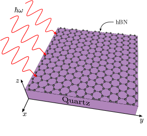
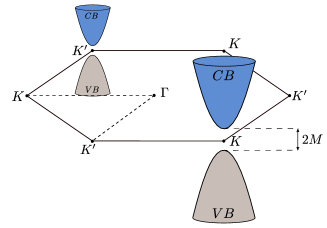
Figure 1: Representation of the experimental setup and Brillouin zone of hBN. The top image shows the experimental setup: a hBN layer on quartz with photons shining on the system. On the bottom image we represent the hexagonal Brillouin zone of hBN together with the gapped Dirac cones existing at the edges of the zone; the bare (without exchange corrections) energy gap is $2M$.

The paper is organized as follows: In Sec.2, we develop the needed formalism for the calculation of the excitonic response of hBN on quartz. In Sec.3, we provide results for the absorption of hBN as function of frequency and show that the material can support both TE and TM exciton-polaritons of large wave number and, therefore, with a high degree of confinement. In Sec.4, we compute the spontaneous emission decay rate of excitons in hBN on quartz, a quantity essential for the interpretation of photoluminescent experiments. Finally, in the Appendix, we present some useful formulae used in the numerical part of our analysis and benchmark the method against known analytical results.

2 Formalism

In this section we introduce the electronic model Hamiltonian and present the formalism for solving the 2D Wannier equation with an attractive electron-hole interaction described by the Rytova-Keldysh potential [25, 26]. We also show how this Wannier equation can be obtained from the Bethe-Salpeter equation by means of a Fourier transform.

2.1 Model Hamiltonian for hBN

The electronic and optical properties of electrons in the hybridized $p_{z}$ orbitals of hBN are well described by a first-neighbor tight-binding model. This can be further simplified by writing a low energy model around the Dirac points, located at the corners of the Brillouin zone. This low energy model is, in this case, a massive Dirac equation in 2D, with an Hamiltonian given by:

$$H_{0}=v_{F}\hbar\mathbf{k}\cdot\bm{\sigma}+M\sigma_{z}\,,$$ (1)

for $v_{F}$, the Fermi velocity; $\mathbf{k}=(k_{x},k_{y})$ is the in-plane wave vector of the electrons in the hybridized $p_{z}$ orbitals; $\bm{\sigma}=(\sigma_{x},\sigma_{y})$, with $\sigma_{j}$ the $j=x,y,z$ Pauli matrix: and $2M$ is the density functional theory (DFT) band gap (e. g., at the LDA level of approximation) at the corners of the Brillouin zone. We note that the Pauli matrices do not refer to real spin but rather to the basis of the hexagonal lattice unit cell. The eigenproblem $H_{0}|u_{\mathbf{k},s}\rangle=E_{s}|u_{\mathbf{k},s}\rangle$, with $s=\pm,$ has a simple solution, reading

$$|u_{\mathbf{k},+}\rangle = \frac{1}{\sqrt{2E_{+}}}\left(\begin{array}[]{c}\sqrt{M+E_{+}}\\ \frac{v_{F}\hbar ke^{i\theta}}{\sqrt{M+E_{+}}}\end{array}\right)$$ (7)

$$\underset{k\rightarrow 0}{\longrightarrow}\frac{1}{\sqrt{2M}}\left(\begin{array}[]{c}\sqrt{2M}\\ \frac{v_{F}\hbar ke^{i\theta}}{\sqrt{2M}}\end{array}\right)\,,$$

and

$$|u_{\mathbf{k},-}\rangle = \frac{1}{\sqrt{2E_{+}}}\left(\begin{array}[]{c}-\frac{v_{F}\hbar ke^{-i\theta}}{\sqrt{M+E_{+}}}\\ \sqrt{M+E_{+}}\end{array}\right)$$ (13)

$$\underset{k\rightarrow 0}{\longrightarrow}\frac{1}{\sqrt{2M}}\left(\begin{array}[]{c}-\frac{v_{F}\hbar ke^{-i\theta}}{\sqrt{2M}}\\ \sqrt{2M}\end{array}\right)\,,$$

with $E_{s}=s\sqrt{M^{2}+v_{F}^{2}\hbar^{2}k^{2}}$ (at spaces we also use $s=c/s$ when used as an index).

The asymptotic expression of the spinors when $k\rightarrow 0$ will be used in the calculation of the radiative lifetime of the exciton. We note that this approximation is justified by the fact that the energy gap in hBN is rather large $\sim 4$ eV (in the absence of exchange corrections. These corrections further widen the gap).

The total electronic Hamiltonian is the sum of $H_{0}$ with the Rytova-Keldysh interacting potential:

$$V(r)=\frac{e^{2}}{4\pi\epsilon_{0}}\frac{\pi}{2}\frac{1}{r_{0}}\left[H_{0}\left(\frac{\epsilon_{1}r}{r_{0}}\right)-Y_{0}\left(\frac{\epsilon_{1}r}{r_{0}}\right)\right]\,,$$ (14)

where $r_{0}$ is a length scale of the order of $r_{0}\sim\epsilon_{2}d/2$, with $d$ the thickness of the 2D material, and $\epsilon_{2}$ the dielectric function of the 2D material film; $\epsilon_{1}$ is the dielectric function of the medium surrounding the 2D material; $H_{0}(x)$ is the Struve function and $Y_{0}(x)$ is the Bessel function of the second kind. This form of the potential follows from the solution of Laplace equation for a thin film embed in a medium. If the 2D material is encapsulated between two different dielectrics, $\epsilon_{1}$ and $\epsilon_{3}$, then it is necessary to replace $\epsilon_{1}$ in Eq. 14 by the arithmetic mean of the two dielectric functions.

2.2 Derivation of the Wannier equation in 2D

In second quantization, the state of an exciton of momentum $\mathbf{Q}$, in motion in an hBN layer of area $A$, can be expressed by

$$|\nu,\mathbf{Q}\rangle=\frac{1}{\sqrt{A}}\sum_{\mathbf{k}}\phi_{\nu}(\mathbf{k})a_{\mathbf{k}+\mathbf{Q},c}^{\dagger}a_{\mathbf{k},v}|GS\rangle,$$ (15)

where the state $|GS\rangle$ represents the electronic ground state of hBN, that is, a fully occupied valence band and an empty conduction band. Also, $\phi_{\nu}(\mathbf{k})$ is the Fourier transform of the real space exciton wave function characterized by the set of quantum numbers $\nu$ (in our case it will be the principal and magnetic quantum numbers). The second quantized operators $a_{\mathbf{k}+\mathbf{Q},c}^{\dagger}$ and $a_{\mathbf{k},v}$ create and annihilate an electron of momentum $\mathbf{k+\mathbf{Q}}$ in the conduction band and an electron of momentum $\mathbf{k}$ in the valence band, respectively. This state can then be expressed as $|\nu,\mathbf{Q}\rangle=b_{\mathbf{Q},\nu}^{\dagger}|GS\rangle,$ for $b_{\mathbf{Q},\nu}^{\dagger}$ the a bosonic operator,

$$b_{\mathbf{Q},\nu}^{\dagger}=\frac{1}{\sqrt{A}}\sum_{\mathbf{k}}\phi_{\nu}(\mathbf{k})a_{\mathbf{k}+\mathbf{Q},c}^{\dagger}a_{\mathbf{k},v}.$$ (16)

This representation will be useful in the calculation of the radiative lifetime of the exciton. We also note that the bosonic nature of the operator (16) is guaranteed only in an average over the ground state.

The Hamiltonian describing the electrons in hBN can then written in second quantization as

$$H=H_{0}+V\,,$$ (17)

with

$$H_{0}=\sum_{\lambda,\mathbf{k}}E_{\lambda,\mathbf{k}}\hat{a}_{\lambda,\mathbf{k}}^{\dagger}\hat{a}_{\lambda,\mathbf{k}}\,,$$ (18)

where $\lambda=c,v$, and $E_{\lambda,\mathbf{k}}=E_{s}$, and with the interaction term given by

$$V = \frac{1}{2A}\sum_{\mathbf{k}_{1},\mathbf{k}_{2},\mathbf{p}}\sum_{\lambda_{1}\lambda_{2}\lambda_{3}\lambda_{4}}V(\mathbf{p})F_{\lambda_{1}\lambda_{2}\lambda_{3}\lambda_{4}}(\mathbf{k}_{1},\mathbf{k}_{2},\mathbf{p})$$ (19)

$$\times \hat{a}_{\mathbf{k}_{1}+\mathbf{p},\lambda_{1}}^{\dagger}\hat{a}_{\mathbf{k}_{2}-\mathbf{p},\lambda_{2}}^{\dagger}\hat{a}_{\mathbf{k}_{2},\lambda_{3}}\hat{a}_{\mathbf{k}_{1},\lambda_{4}}\,,$$

and

$$F_{\lambda_{1}\lambda_{2}\lambda_{3}\lambda_{4}}(\mathbf{k}_{1},\mathbf{k}_{2},\mathbf{p})=u_{\mathbf{k}_{1}+\mathbf{p},\lambda_{1}}^{\dagger}u_{\mathbf{k}_{2}-\mathbf{p},\lambda_{2}}^{\dagger}u_{\mathbf{k}_{2},\lambda_{3}}u_{\mathbf{k}_{1},\lambda_{4}}\,,$$ (20)

is a product of spinors (7) and (13) and is termed the form factor. The function $V(\mathbf{p})$ is the Fourier transform of the Rytova-Keldysh potential (14) is known analytically [25], and it is given by $V(\mathbf{q})=e^{2}/[2\epsilon_{0}q(r_{0}q+\epsilon_{1})]$. Next we show that if the state (15) is an eigenstate of $H$, then $\phi_{\nu}(\mathbf{k})$ obeys the Bethe-Salpeter equation and its Fourier transform to real space gives rise to the Wannier equation.

In order to obtain the Bethe-Salpeter equation we proceed as follows: we assume that the state (15) is an eigenstate of the Hamiltonian $H$. If this is the case, then $H$ can be written as $H=\sum_{\mathbf{Q},\nu}E_{\mathbf{Q},\nu}b_{\mathbf{Q},\nu}^{\dagger}b_{\mathbf{Q},\nu}$, where $E_{\mathbf{Q},\nu}$ are the energy eigenvalues of the exciton. Next we compute the commutator of $H$ with $b_{\mathbf{Q},\nu}^{\dagger}$ using both the fermionic and bosonic representations. In the end we must demand both results be the same. Proceeding as such, we obtain the following equation for the wave function of the exciton in momentum space:

$$E\phi_{\nu}(\mathbf{k})=\phi_{\nu}(\mathbf{k})(E_{c,\mathbf{k}}-E_{v,\mathbf{k}})+\frac{1}{A}\phi_{\nu}(\mathbf{k})\sum_{\mathbf{p}}V(\mathbf{p})\times$$

$$\left[u_{\mathbf{k},v}^{\dagger}u_{\mathbf{k-p},v}^{\dagger}u_{\mathbf{k},v}u_{\mathbf{k-p},v}-u_{\mathbf{k},c}^{\dagger}u_{\mathbf{k+p},v}^{\dagger}u_{\mathbf{k},c}u_{\mathbf{k+p},v}\right]$$

$$-\frac{1}{A}\sum_{\mathbf{p}}V(\mathbf{p})\phi_{\nu}(\mathbf{p+k})u_{\mathbf{p+k},v}^{\dagger}u_{\mathbf{k},c}^{\dagger}u_{\mathbf{p+k},c}u_{\mathbf{k},v}\,,$$ (21)

where $E$ represents the exciton energy eigenvalues. The latter equation — an eigenvalue equation in momentum space for $\phi_{\nu}(\mathbf{k})$ — is known as the Bethe-Salpeter equation. The physics of the different terms is clear: the first term is the energy when a particle-hole excitation is created, in the non-interacting limit. The second term represents the exchange energy correction to the non-interacting particle-hole excitation energy (its value determines the magnitude of the gap), the third and final term represents the attraction between the electron created in the conduction band and the hole left behind in the valence band. Crucially this term in negative, although in original Hamiltonian the interaction between electrons is obviously repulsive. Note that, although this problem can be solved directly in the momentum space, it involves an integral equation for $\phi_{\nu}(\mathbf{k})$, whose solution can be rather delicate [24], as the sum over the wave vector ranges over an infinite area in the reciprocal space. Another approach is to transform this integral equation into a differential one going to real space. Now, Fourier transforming this equation is also no simple task (and virtually an impossible one) due to the presence of the spinors. To do so, we make the following observation concerning the form factors in the Bethe-Salpeter equation. In the case of a large energy gap, one can take,

$$u_{\mathbf{p+k},v}^{\dagger}u_{\mathbf{k},c}^{\dagger}u_{\mathbf{p+k},c}u_{\mathbf{k},v}\longrightarrow 1+\mathcal{O}\left(1/M^{2}\right)\,.$$ (22)

so as to forego the spinorial structure of the last term of the Bethe-Salpeter equation. It is also considered that both the energy difference, $E_{c,\mathbf{k}}-E_{v,\mathbf{k}}$, and the exchange energy corrections are expanded up to second order in $\mathbf{k}$. The resulting differential equation — in real space — reads as,

$$(E-E_{g})\psi_{\nu}(\mathbf{r})=-\bigg{[}\frac{\hbar^{2}}{2\mu}\nabla^{2}+V(\mathbf{r})\bigg{]}\psi_{\nu}(\mathbf{r})\,,$$ (23)

which is known as the Wannier equation for the excitonic wave function. Here $\mu$ is the reduced mass of the exciton which, in our model, reads $m^{\ast}/2$. The quantity $E_{g}$ (termed free particle band gap) reads $E_{g}=2M+\Delta_{ex}$, for $\Delta_{ex}$, the exchange energy correction to the DFT gap evaluated at $\mathbf{k}=0$. This correction is given by,

$$\Delta_{ex} = \frac{\alpha M}{r_{0}}\frac{c}{v_{F}}\frac{{\rm arcsinh}\frac{\epsilon_{1}v_{F}\hbar}{r_{0}M}+{\rm arcsinh}\frac{r_{0}M}{\epsilon_{1}v_{F}\hbar}}{\sqrt{\Big{(}\frac{\epsilon_{1}}{r_{0}}\Big{)}^{2}+\Big{(}\frac{M}{v_{F}\hbar}\Big{)}^{2}}}$$ (24)

$$\approx \frac{\alpha\hbar c}{r_{0}}\log\frac{2Mr_{0}}{\epsilon_{1}v_{F}\hbar}+\frac{\alpha\epsilon_{1}\hbar^{2}v_{F}c}{r_{0}^{2}M}\,,$$

where $\alpha$ is the fine structure constant. The approximate result holds for $Mr_{0}\gg\epsilon_{1}\hbar v_{F}$, for $\epsilon_{1}$, the average value of the dielectric functions of the substrate and capping layer.

In the next section we describe a semi-analytical method of solving the Wannier equation, whose solutions will allow us to easily access the optical properties of 2D materials.

2.3 An efficient method for solving the Wannier equation in 2D

We have shown in the previous section that solving the excitonic problem requires the determination of the exciton wave function in both real and reciprocal spaces. As such, it would be convenient that the wave function could be expressed in a form that would ease the calculations, as a fully numerical approach usually renders the calculation numerically expensive. Here, we show that a quasi-analytical expression for the wave functions of the exciton can be written using a set of Gaussian functions. The initial idea is relatively simple: in solid state physics, DFT calculations of the band structure of solids are routinely performed in different basis sets — plane-waves, Slater-type orbitals, and Gaussian functions being the most commonly used. Plane waves are clearly not suitable for our problem, as we are dealing here with bound-states. The Slater basis has the advantage of describing the behavior of the wave functions near the origin in a very precise manner, but it is computationally demanding when the matrix elements of the kinetic operator have to be determined. The basis of Gaussian functions requires considerably more terms to describe the behavior of the wave function near the origin, but has the advantage of allowing for analytical expressions for the matrix elements of both the kinetic energy operator and the electron-electron interacting potential. This latter choice of basis is the approach used in this this paper. Drawing inspiration from the solution of the 2D hydrogen atom (see Appendix), we write our wave function in the form:

$$\psi_{\nu}(\mathbf{r})=\mathcal{A}_{\nu}\sum_{j=1}^{N}c_{j}^{\nu}e^{im\theta}r^{|m|}e^{-\zeta_{j}r^{2}}\,,$$ (25)

Note that $e^{im\theta}r^{|m|}$ follows from the eigenfunctions of the $z-$component of the angular momentum and describes the wave function near the origin, for $m=0,\pm 1,\pm 2,\ldots$, the magnetic quantum number; the Gaussian term $e^{-\zeta_{j}r^{2}}$ describes the decay of the wave function at large distances, with with a decay constant that depends on $\zeta_{j}$. The coefficients $c_{j}^{\nu}$ are weights for the different Gaussians; whereas ${\cal A}_{\nu}$ is a normalization constant. An additional advantage of this method is that the matrix elements of both the kinetic operator and the electron-electron interaction do not mix different $m$ values and therefore, the eigenvalue problem is block diagonal in the angular momentum space. The quantum number $\nu$ plays the role of the principal quantum number: for each value of $m$ there is an infinite number of $\nu$’s (note, however, that we also use the label $\nu$ for denoting both the magnetic and the principal quantum numbers together).

Using our trial wave function and computing the matrix elements of the kinetic and potential energy operators, the generalized eigenvalue problem acquires the form

$$\sum_{j=1}^{N}[H(\zeta_{i},\zeta_{j})-S(\zeta_{i},\zeta_{j})E]c_{j}^{\nu}=0,$$ (26)

where $H(\zeta_{i},\zeta_{j})$ is called the Hamiltonian kernel and $S(\zeta_{i},\zeta_{j})$ is the superposition kernel. This differs from a Kronecker$-\delta$ kernel since the set of Gaussian functions is not an orthogonal basis. Both kernels have an analytical expression given in the Appendix. Equation (26) has first been written in nuclear physics and is termed the Griffin-Hill-Wheeler equation [27]. The normalization constant is determined in the usual way and reads

$$\mathcal{A}_{\nu}=\sqrt{\frac{1}{\pi\>\mathcal{S}_{\nu}}}\,,$$ (27)

with $\mathcal{S}_{\nu}=\sum_{j=1}^{\infty}\sum_{j^{\prime}=1}^{\infty}c_{j}^{\nu*}c_{j^{\prime}}^{\nu}(\zeta_{j}+\zeta_{j^{\prime}})^{-1-|m|}\Gamma(|m|+1)$, and $\Gamma(x)$ the gamma-function. A critical aspect of the method is the judicious choice of the parameters $\zeta_{j}$. A choice not so well known is the use of a logarithmic grid of $\zeta^{\prime}s$ according to the rule [28]

$$\Omega=\frac{\ln\zeta}{A},\qquad A>1\,,$$ (28)

where the $\Omega^{\prime}s$ are uniformly distributed in an interval $[\Omega_{{\rm min}},\Omega_{{\rm max}}]$ and $A$ is typically chosen in the interval $[6,8].$ With the method exposed, we move on to the calculation of the eigenvalues and eigenvectors of the Griffin-Hill-Wheeler equation for both the Coulomb (see Appendix) and the Rytova-Keldysh potentials. In Table 1, we present the spectrum of the Rytova-Keldysh potential in the conditions discussed in Sec. 3. In Fig. 2, we depict a set of solutions of Eq. (26) for both the Rytova-Keldysh and Coulomb potentials, where again used the conditions of the following section. In Table 1 we present the bound state energies for different reduced masses $\mu$: as $\mu$ decreases the kinetic energy increases and the states become less bound.

$m^{\ast}$	principal q.n.	$n=1$	$n=2$	$n=3$	$n=4$
$m_{0}$	Energy (eV)	-0.992	-0.274	-0.126	-0.072
$0.7m_{0}$	Energy (eV)	-0.845	-0.213	-0.094	-0.052
$0.5m_{0}$	Energy (eV)	-0.718	-0.155	-0.071	-0.0314

Table 1: Energy spectrum of the Rytova-Keldysh potential for hBN on quartz, with $r_{0}=10$ Å  and with the average dielectric function of substrate and capping layer taken to be $\epsilon_{1}=2.4$, that is, the substrate is quartz and the capping layer is air. Different values of the effective mass $m^{\ast}$ have been considered. The calculation used $100$ Gaussians and the first four energy eigenvalues labeled by the princial quantum number (q.n.) $n$ are given (they all correspond to the $m=0$ case).

Figure 2: Few radial wave functions of the Rytova-Keldysh and Coulomb potentials for the parameters of Table 2. With the given set of parameters the wave functions of the Rytova-Keldysh potential are more spread out in space, which imply larger (less bound) energy values (compare values of Table 1 and Table 5). The calculation used an effective mass $m^{\ast}=0.6m_{0}$.

3 Results

In this section, we compute the absorption of hBN on quartz. We also discuss the existence of surface exciton-polaritons and their application in sensors.

3.1 Absorption of hBN: Theory

The calculation of the absorption of hBN requires the calculation of the reflection, ${\cal R}$, and transmission, ${\cal T}$, coefficients, with the absorption defined as

$${\cal A}=1-{\cal R}-\Re(\sqrt{\epsilon_{3}/\epsilon_{1}}){\cal T}.$$ (29)

The determination of ${\cal R}$ and ${\cal T}$ requires the solution of the Fresnel problem (that is, the scattering of electromagnetic radiation by a flat interface) when a 2D material is embed in two different dielectrics. From the solution of the Fresnel problem at normal incidence the absorption is given by Eq. (29) with ${\cal R}=|r|^{2}$ and

$$r=\frac{\sqrt{\epsilon_{3}}-\sqrt{\epsilon_{1}}+\sigma/(\epsilon_{0}c)}{\sqrt{\epsilon_{3}}+\sqrt{\epsilon_{1}}+\sigma/(\epsilon_{0}c)}\,,$$ (30)

and ${\cal T}=|t|^{2}$, with

$$t=\frac{2\sqrt{\epsilon_{1}}}{\sqrt{\epsilon_{3}}+\sqrt{\epsilon_{1}}+\sigma/(\epsilon_{0}c)}\,,$$ (31)

with $\epsilon_{1}$ and $\epsilon_{3}$ the dielectric functions of air and quartz, respectively, and $\sigma=\sigma(\omega)$ is the optical conductivity of the 2D material, which can be obtained by usual perturbation theory. After a lengthy calculation we obtain,

$$\frac{\sigma}{\sigma_{0}}=\frac{i}{4\pi^{3}}\sum_{\nu}|E_{g}+E_{\nu}|\Lambda_{\nu}\left(\frac{1}{\hbar\omega+E_{\nu}+E_{g}+i\eta}+\right.$$

$$\left.\frac{1}{\hbar\omega-E_{\nu}-E_{g}+i\eta}\right)\,,$$ (32)

where $\Lambda_{\nu}$ is roughly proportional to the square modulus of the wave function of the exciton; $E_{g}$ is the gap between the valence and the conduction bands (often called the free particle band gap to distinguish it from the the optical band gap, the latter determined by excitons) after the inclusion of the exchange energy correction; $E_{\nu}$ is the exciton energy level associated with the quantum number $\nu$ (including both the principal and magnetic quantum numbers). Only three magnetic quantum numbers produce a non-zero result, $m=0$ and $m=\pm 2$, the largest contribution being, by far, that of $m=0$; finally, $\eta$ is the non-radiative decay rate, encompassing all possible decay channels. The conductivity here is expressed in units of graphene universal conductivity $\sigma_{0}=e^{2}/(4\hbar)$. Using Eq. (32) in Eq. (29) the absorption of hBN can be computed. This is given in Fig 3. The parameters used in the theoretical calculations are given in Table 2. As for the non-radiative decay rate, $\eta$, it is a fitting parameter and whose microscopic calculation is beyond the present study, as it requires calculations taking into account electron-impurity, electron-phonon and electron-electron scattering processes. In practical terms, the value of $\eta$ controls the intensity of the absorption curve. For the dielectric function of quartz in the ultraviolet, we have used the experimentally tabulated values. We note that the electron-electron interaction depends on the static dielectric function of quartz, $\epsilon_{{\rm quartz}}$, whereas the absorption depends on the dynamic dielectric function, $\epsilon(\omega)$.

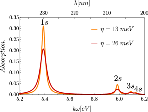
Figure 3: Absorption of hBN on quartz. In principle there is only one fitting parameter, the non-radiative decay rate $\eta$, which was chosen as $\eta=13$ meV. The value of the free particle band gap is given by $E_{g}=2M+\Delta_{ex}$, which has been computed to be $6.2$ eV, for hBN on quartz, and $7.2$ eV for hBN in vacuum, using the parameters of Table 2. An effective mass of $m^{\ast}=0.6m_{0}$ was used, where $m_{0}$ is the bare electron mass. The effect of changing the reduced mass is discussed in Table 1. The Rydberg series of the excitonic spectrum is clearly seen.

$\mathbf{N}$	$\mathbf{\Omega_{min}}$	$\mathbf{\Omega_{max}}$	$\mathbf{A}$	$\mathbf{E_{g}}$ (eV)	$\mathbf{M}$ (eV)	$\mathbf{\hbar v_{F}}$ (eV$\cdot$Å)	$\bm{\eta}$ (eV)	$\mathbf{r}_{0}$ (Å)	$\epsilon_{{\rm quartz}}$
100	-2	5	6	6.17	1.96	5.06	0.013	10	3.9

Table 2: Parameters used in the calculation of the excitonic conductivity of hBN. The parameters $r_{0}$, $M$, and $\hbar v_{F}$ where extracted from Ref. [22]. The parameter $\epsilon_{{\rm quartz}}$ refers to the static dielectric constant of quartz that enters in the Rytova-Keldysh potential. The parameters $N$, $\Omega_{{\rm min}}$, $\Omega_{{\rm max}}$, and $A$ were chosen with the criteria of reproducing accurately the analytical 2D energy spectrum and wave functions of the attractive Coulomb problem. We have varied these set of parameters and checked that significant variations do not alter the final result. The non-radiative decay rate $\eta$ is a fitting parameter and its microscopic calculation is beyond the scope of the present study.

As given above, we have determined an analytical expression for the exchange energy correction to the DFT band gap from Eq. (24) and have found that the new gap, $E_{g}=2M+\Delta_{ex}$, reads $\sim 6.2$ eV for hBN on quartz. For hBN in vacuum, we found that $E_{g}=2M+\Delta_{ex}\sim 7.2$ eV. This value is in agreement with DFT+GW calculations, as can be seen in Table 3. We note in passing that a calculation of the exchange energy was made in Ref. [24] in the context of the absorption of electromagnetic radiation by TMD and the resulting energy gap $E_{g}$ was shown to be in excellent agreement with the experimental data.

Ref.	[33]	[34]	[35]	[36]	[37]	this work
$E_{g}$ (eV)	7-7.5	7.25	8($\dagger$)	6.46	7.4	7.2,8.0$(\ast)$

Table 3: Theoretical energy gap parameter, $E_{g}$, computed in different references. ($\ast$) Values in vacuum for $r_{0}=10,6.9\,$Å, respectively (see also Table 4). ($\dagger$) Direct gap; these authors found an indirect band gap of 7.74 eV for the monolayer. (The value of $E_{g}$ on quartz was found by us to be $E_{g}\approx 6.2$ eV.)

3.2 Photoluminescence of hBN on graphite

For putting our theory to the test, we have compared the theoretical position of the excitonic energy levels of a hBN single-layer to photoluminescence (PL) of hBN single layer on highly oriented pyrolytic graphite (HOPG), published very recently [30]. In this paper, the authors were able to measure the PL of a single hBN layer in the frequency range $\lambda\in[240,200]$ nm, at a temperature of 10 K. They identified a broad deep-ultraviolet emission in the region $\lambda\in[240,210]$ nm. This type of emission is, traditionally, attributed to to excitons trapped in defects of the hBN lattice [5], energetically located inside the gap, and is termed, in bulk hBN, the $D-$series ($D$ from diffuse) [31]. In addition to this, those authors identified two sharp peaks ($S-$series) in the region $\lambda\in[210,200]$ nm. This emission is attributed to excitons. To explain the data of Ref. [30], we have computed absorption (which depends directly on the position of the excitonic energy levels) of a single hBN layer on HOPG, which can, to first approximation be considered as a perfect conductor. This fact leads to screening the Rytova-Keldysh potential, which has an approximate analytical solution for $d\ll r_{0}$:

$$V(\mathbf{r}) = \frac{e^{2}}{\epsilon_{0}}\int_{0}^{\infty}\frac{dq}{2\pi}J_{0}(qr)\left[2r_{0}q+\frac{e^{qd}}{\sinh(qd)}\right]^{-1}$$ (33)

$$\approx \frac{e^{2}}{4\pi\epsilon_{0}r_{0}}K_{0}(r/\sqrt{2dr_{0}})\,,$$

with $d$ the distance between hBN and HOPG substrate and $K_{0}(x)$ the modified Bessel function. We have verified numerically that for hBN at a distance of $d=3.5$Å  of the HOPG substrate (this distance corresponds to the measured step height (3.5Å) between HOPG and hBN [30, 32] using AFM), the screened potential is well described by the approximation in Eq. (33), although slightly more attractive. In addition, for the approximated screened potential, the exchange energy also has an analytical form:

$$\Delta_{ex}^{scr}=-i\frac{\sqrt{2d}M\alpha\hbar c\,{\rm arccos}\frac{M\sqrt{2dr_{0}}}{\hbar v_{F}}}{\sqrt{r_{0}}\sqrt{2dr_{0}M^{2}-\hbar^{2}v_{F}^{2}}}\,,$$ (34)

with the corrected gap given by $E_{g}^{src}=2M+\Delta_{ex}^{src}$ and the constraint $2dr_{0}M^{2}>\hbar^{2}v_{F}^{2}$; the Fourier transform of $V(\mathbf{r})$ given by Eq. (33) reads $V(\mathbf{q})=4\pi\hbar c\alpha(1/q)[2r_{0}q+1/(qd)]^{-1}$.

$n=1$	$E_{g}^{scr}$ (eV)	$r_{0}\,$(Å)	$d\,$(Å)
-1.546 eV	7.6($\ast$)	6.9($\dagger$)	3.5

Table 4: Excitonic energy levels of hBN at a distance of $3.5$Å  from a highly conductive HOPG substrate (a value fixed by the experimental measured distance using AFM). The energy level is depicted in Fig. 4 as peaks in the absorbance spectrum. The effective mass of the electrons is $m^{\ast}=0.6m_{0}$. Note that we have changed $r_{0}$ relative to the value give in Table 2. This was necessary for making the $1s-$level coincident with the excitonic peak in the PL data of Fig. 4. However, this choice of $r_{0}$ is consistent with the available data in the literature. Indeed, the value of $r_{0}$ can be estimated from [38] $r_{0}=(\sqrt{\epsilon_{\perp}\epsilon_{\parallel}}-1)d/2=6.5$, with $\epsilon_{\perp}=3.29$ and $\epsilon_{\parallel}=6.82$ [29]. If, on the other hand, we use the results of Refs. [39, 40], we find $r_{0}=(\kappa-1)d/2=6.8$, with $\kappa=4.9$. Both results for $r_{0}$ are in approximate agreement with our choice. ($\ast$) The gap in vacuum for $r_{0}=6.9$Å  reads $E_{g}=$7.97 eV, larger than in the presence of the HOPG, as it should be. We note that, incidentally, this value of $E_{g}$ coincides with that of Refs. [35, 39] (see Table 3). ($\dagger$) A self-consistent calculation using no approximations to the screened potential and with $r_{0}$ determined via a RPA calculation, gives $r_{0}=7.2$Å  and $E_{g}^{scr}\approx 7.2$ eV [41].

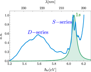
Figure 4: Experimental photoluminescence (blue line) [30] and theoretical resonant absorption showing a peak at the energy level $n=1$ given in Table 4. An effective mass $m^{\ast}=0.6m_{0}$ was used, in agreement with the estimations made in Sec. 1. Both the absorption (theory) and the PL spectrum (experiment) have been normalized to their maximum value. The computed gap with exchange corrections reads $E_{g}^{src}=7.6$ eV. A value of $\eta=30$ meV has been used, in agreement with the experimental measurements [30] at 10 K. The diffuse series ($D-$series) is due to excitons trapped in defects forming inside the gap; the sharp series ($S-$series) is due to (free) excitons.

The result of our calculation is given in Table 4 and depicted in Fig. 4 together with the PL data. Our calculation reveals a single excitonic $s-$level given by the value of Table 4. The $1s$ level coincides with the $S-$series. For the approximated form of the interaction potential only the $1s$ bound state exists. Finally, we note that the double peak seen in the experiment is due to out-of-plane phonons coupling an electron in the valley $\mathbf{K}$ and a hole in the valley $\mathbf{K}^{\prime}$, or vice-verse. Our theory does not take phonons into account therefore is unable to describe the peak splitting. We stress that the apparent increase of PL near $200$ nm seen in the PL data is due to stray light from the excitation laser and is not an excitonic effect.

3.3 Exciton-polaritons in hBN

As discussed in the Introduction, some peptides have a strong absorption at the frequency of the excitonic resonances of hBN on quartz. When this situation happens a sensor working in the corresponding spectral range is conceivable. A widely used type of sensor is based on the concept of polariton, and it is associated to two of its fundamental properties: (i) an evanescent decay of the electromagnetic field around the surface of the 2D material; (ii) an enhancement of electromagnetic field in the vicinity of the 2D material. These two properties should allow the determination of very small changes in the refractive index of the medium surrounding the 2D material and should, therefore, work as a sensor of small quantities of analyte.

There are different kinds of polaritons: phonon-polaritons, plasmon-polatirons, magnon-polaritons, and exciton-polaritons. All of them have in common the two properties mentioned above. In our case, we are concerned with the exciton-polariton. We shall show below that the electromagnetic field of the polariton is concentrated within few nanometers from the surface of hBN.

In what concerns their polarization, there can be two different types of exciton-polaritons: transverse electric (TE) and transverse magnetic (TM). The first kind is possible when the imaginary part of the excitonic optical conductivity is negative, whereas the second kind happens in the opposite case, when the imaginary part of the excitonic optical conductivity is positive. The dispersion relations of the two kinds of excitons are very different from one other. For TE exciton-polaritons the implicit expression for the dispersion relation reads,

$$\kappa_{1}+\kappa_{2}-i\omega\mu_{0}\sigma(\omega)=0\,,$$ (35)

whereas for TM polarization we have,

$$\frac{\epsilon_{1}}{\kappa_{1}}+\frac{\epsilon_{2}}{\kappa_{2}}+i\frac{\sigma(\omega)}{\epsilon_{0}\omega}=0\,,$$ (36)

where $\epsilon_{j}$, with $j=1,2$, the relative dielectric permittivity of the two media cladding the hBN layer; $\kappa_{j}=\sqrt{q^{2}-\epsilon_{j}\omega^{2}/c^{2}}$, $\omega$ is the frequency of the exciton-polarion electromagnetic field; $c$ is the speed of light in vacuum; $q$ is the in-plane wave vector of the polariton; and $\epsilon_{0}$ and $\mu_{0}$ are the vacuum dielectric permittivity and magnetic permeability, respectively. The solutions to the two previous equations give the dispersion relations, $\omega(q)$, for the two possible polarizations. In Fig. 5, we depict both the TE and TM dispersion of the polariton. The lowest branch refers to the TE polarization and the other branch to the TM polarization. They both show large deviations from the light-line, which leads to a strong confinement of the exciton-polations — as $q$ grows the exciton-polariton wavelength $\lambda_{ep}=2\pi/q$ decreases, leading to spatial localization of the exciton-polariton. A further look at Fig. 5 shows that the TM branch has wave numbers that are much larger than those of the TE branch and, therefore, is prone to a larger degree of confinement.

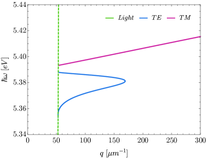
Figure 5: Spectrum of the TE and TM exciton-polaritons. We stress that the calculation has taken into account both the real and the imaginary parts of the optical conductivity of hBN. The spectrum shown is due to the contribution of the $1s-$exciton alone.

In Fig. 6, we depict in the top (bottom) panel the electromagnetic field of the TE (TM) exciton-polaritons. We can see the electromagnetic field is concentrated within the scale of few nanometers ($\sim 10$ nm) for both the TE and TM modes. For the TM mode, one can have a larger degree of spatial confinement. This difference is explained by the spectrum shown in Fig. 5 which shows that is possible to have TM polarized polaritons that have a larger wave number than those that are TE polarized. This characteristic — the strong degree of confinement — makes the polariton field extremely sensitive to small changes of the dielectric function of the medium in contact with the 2D material in the UV range.

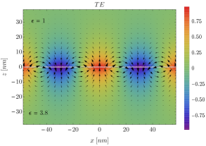
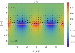
Figure 6: Spatial maps of the electromagnetic field of both TE (top) and TM (bottom) polaritons. For the TE polariton the vector field is that of the magnetic field and the intensity refers to the single components of the electric field. For the TM polariton the vector field is that of the electric field and the intensity refers to the single component of the magnetic field of the polariton. The parameters used were: $\epsilon_{1}=1$, $\epsilon_{2}=3.8$, $q=104\;\mu{\rm m}^{-1}$ and $\hbar\omega=5.386\quad{\rm eV}$ for the TE spatial map (top image), and $q=107\;\mu{\rm m}^{-1}$ and $\hbar\omega=5.398\quad{\rm eV}$, for the TM spatial map (bottom image).

4 The spontaneous radiative decay rate of excitons in hBN

In this section, we provide the calculation of the spontaneous radiative decay rate of excitons in hBN. Incidentally, the formula used here could also be useful for the calculation of this decay recay for the transition-metal dichalcogenides (upon some trivial modifications, that is, considering the spin-orbit band splitting). For computing the spontaneous radiative decay rate it is convenient to formulate the problem in second quantization, both for the excitonic Hamiltonian and for the photon field. For simplicity, we assume that the hBN layer is in a medium of dielectric permittivity $\epsilon$. In term of exciton operators $b_{\mathbf{Q},\nu}$ and $b_{\mathbf{Q},\nu}^{\dagger}$ the interaction Hamiltonian of the exciton with the electric field of the photon reads,

$$H_{int}=e\sqrt{A}\sum_{\nu}\mathbf{E}\cdot\bm{\Phi}_{\nu}^{\ast}b_{\mathbf{0},\nu}^{\dagger}+e\sqrt{A}\sum_{\nu}\mathbf{E}\cdot\bm{\Phi}_{\nu}b_{\mathbf{0},\nu}\,,$$ (37)

where $\mathbf{E}$ is the photon field given by,

$$\mathbf{E}(\mathbf{r},t)\approx i\sum_{\mathbf{q}}\sum_{\iota=1}^{2}\sqrt{\frac{\hbar\omega}{2\epsilon\epsilon_{0}V}}[\bm{\epsilon}_{\mathbf{q},\iota}a_{\mathbf{q},\iota}(t)-\bm{\epsilon}_{\mathbf{q},\iota}a_{\mathbf{q},\iota}^{\dagger}(t)]\,,$$ (38)

the vector $\bm{\Phi}_{\nu}$ reads,

$$\bm{\Phi}_{\nu}=\frac{1}{A}\sum_{\mathbf{k}}\phi_{\nu}(\mathbf{k})\bm{\xi}_{\mathbf{k}vc}\,,$$ (39)

with $\nu$ representing both the principal and the magnetic quantum numbers of the exciton, the Berry connection [42, 43] is given by $\bm{\xi}_{\mathbf{k}vc}=-i\langle u_{\mathbf{k},c}|\nabla_{\mathbf{k}}|u_{\mathbf{k},v}\rangle;$ $V$ is the volume of the box enclosing the photon field; $e$ is the elementary charge; $\bm{\epsilon}_{\mathbf{q},\iota}$ is a polarization vector perpendicular to $\mathbf{q}$; $a_{\mathbf{q},\iota}^{\dagger}$ is the creation operator of a photon, while $[a_{\mathbf{q},\iota}^{\dagger}]^{\dagger}=a_{\mathbf{q},\iota}$ is the annihilation operator of a photon. Note that the approximate equality in Eq. (38) follows from the fact that we are considering the electric field to be homogeneous over the size of the exciton, that is $\lambda\gg a_{B}$, where $a_{B}$ is the Bohr radius of the exciton and $\lambda$ the wavelength of the photon. The Berry connection can be computed using the spinors (7) and (13), and leads to:

$$\bm{\xi}_{\mathbf{k}vc}=-i\frac{v_{F}\hbar e^{-i\theta}}{2M}(\hat{u}_{x}e^{i\theta}-e^{i\theta}i\hat{u}_{y}).$$ (40)

Having written the interaction Hamiltonian $H_{int}$ it is now possible — by means of the Fermi golden rule — to calculate the spontaneous radiative decay rate of an exciton in hBN. Since $H_{int}$ depends only on the exciton operator at $\mathbf{Q}=\mathbf{0}$, momentum conservation dictates that the in-plane momentum of the emitted photon has to obey the constraint $(q_{x,}q_{y})=0$. Following this, the radiative decay rate of an exciton with quantum number $\nu$ and wave vector $\mathbf{Q}$ in hBN reads as

$$\frac{1}{\tau_{r}^{\nu,\mathbf{Q}}} = \frac{2\pi}{\hbar}\sum_{\mathbf{q}}|\langle GS;1_{\mathbf{q}}|H_{int}|\nu,\mathbf{Q}\rangle|^{2}$$ (41)

$$\times \delta(\hbar\omega-E(\mathbf{Q})-E_{g}-E_{\nu})\delta_{\mathbf{0},\mathbf{Q}}\delta_{\mathbf{Q},\mathbf{q}_{\parallel}}\,,$$

where $E(\mathbf{Q})=\hbar^{2}Q^{2}/(2m_{CM})$ is the energy of the center of mass of the exciton; $m_{CM}$ is the total mass of the exciton; and $|GS;1_{\mathbf{q}}\rangle$ is the ground state of the semiconductor with an extra photon of momentum $\mathbf{q}$ in the field. The Kronecker$-\delta$, $\delta_{\mathbf{Q},\mathbf{q}_{\parallel}}$, ensures the conservation of the in-plane momentum. We stress that we are computing the spontaneous emission rate of the exciton since we are assuming that there are no photons in the field prior to the decay of the exciton. Calculating the matrix element and integrating over $\mathbf{q}$, finally gives us the radiative decay rate of an exciton in hBN created in a given value,

$$\frac{1}{\tau_{r}^{\nu,\mathbf{0}}}=\alpha\frac{2\pi}{\epsilon\hbar}\frac{v_{F}^{2}\hbar^{2}}{M^{2}}|\psi_{\nu}^{m=0}(\mathbf{r}=0)|^{2}(E_{g}+E_{\nu})\,,$$ (42)

where $\psi_{\nu}^{m=0}(\mathbf{r}=0)$ is the exciton wave function in real space computed at the origin of coordinates with magnetic quantum number $m=0$; $E_{g}$ is the gap in the spectrum at the Dirac points, with the correction introduced by the exchange energy; $\alpha\approx 1/137$ is the fine structure constant; and $\nu$ stands for the principal quantum number. From the parameters of Table 2 we find that $\hbar/\tau_{r}^{0,\mathbf{0}}\approx 30$ meV for hBN in vacuum and $\hbar/\tau_{r}^{0,\mathbf{0}}\approx 4.6$ meV for hBN encapsulated in quartz. Although, at the time of writing, the exciton radiative lifetime in hBN has not yet been measured, the result we obtained is of the order of those found in the TMD, $\hbar/\tau_{r}\sim 4$ meV. The differences should be expected as the TMDs have smaller gaps than that of the hBN. Applying Eq. (42) to MoS₂ in vacuum, we obtained $\hbar/\tau_{r}\approx 4$ meV in agreement with published results [44] and confirmed experimentally [45]. This approach can also be used to determine the temperature dependence of $1/\tau_{r}^{\nu,\mathbf{0}}$. For the case where there are photons in the initial state, as it happens in an experiment illuminated by a continuous-wave laser, the previous expression is to be modified and acquires a prefactor of the form $n_{B}(q)+1$, where $n_{B}(q)$ is the Bose-Einstein distribution function of a photon with wave number $q$. When the temperature rises, the Bose-Einstein distribution function will necessarily grow and the radiative life time decreases.

5 Conclusions

In this paper, we have accurately described the absorption of hBN in the ultraviolet, in the vicinity of excitonic resonance. We have developed a semi-analytical method of solving the Wannier equation based on an expansion of the excitonic wave function in real space in a basis set of Gaussian functions, a method also used in DFT calculations of the band structure of solids. The method reduces the calculation of the energy levels of the exciton and its wave functions to a generalized eigenvalue problem. The solution of the eigenvalue problem determines the coefficients of the expansion of the wave function in the Gaussian basis. Once this problem is solved, the optical properties can be easily computed for any frequency and non-radiative decay rate. The same method can be extended to other 2D materials, with the advantage of being computationally inexpensive. We have also computed the analytical formula for the spontaneous radiative lifetime of the exciton. It is well known [45] that the dielectric susceptibility of a 2D material can be written as

$$\chi(\omega)=\frac{c}{d\omega_{0}}\frac{\gamma_{r}}{\omega_{0}-\omega-i\gamma_{nr}/2}\,,$$ (43)

where $d$ is the thickness of the 2D material, $\omega_{0}$ is the exciton resonance frequency; $\gamma_{nr}$ the non-radiative decay rate (encompassing all possible channels), and $\gamma_{r}$ the radiative decay rate. On the other hand, one can determine the susceptibility, $\chi(\omega)$, by means of the Bethe-Salpeter equation. By this calculation with result of Eq. (43), one can obtain $\gamma_{r}$. We have verified (not shown) that the expression for $\gamma_{r}=1/\tau_{r}^{\nu,\mathbf{0}}$ in Eq. (42) agrees with that found from the Bethe-Salpeter equation.

Finally, we would like to stress that the methods developed in this paper can be applied without restrictions to the study of the optical properties of other 2D materials. The only necessary conditions are the existence of a low energy Hamiltonian that describes the single particle properties, and an energy gap, for implementing the necessary approximations. Of particular interest is the extension of this method to study anisotropic 2D semiconductors such as phosphorene.

Furthermore –and although we discussed the usefulness of hBN exciton-polaritons for the detection of cyclic $\beta-$helical peptides– this same principle can be applied to other biomolecules that have a strong response in the ultraviolet, as long as their resonance frequency does not significantly differ from those found on quartz. Another class of these biomolecules are the $\beta-$Peptoid Foldamers, which also present an optical response in the range $[210\,{\rm nm}-240\,{\rm nm}]$ [46]. By changing the dielectric substrate, one can tune the position of the absorption of h-BN across the range of interest and therefore make from it a viable sensor.

To conclude, we note that our approach can be easily extended to the calculation of nonlinear optical response functions [47] that includes excitonic effects.

Appendix A Numerical solution of the 2D Coulomb problem

In this Appendix, we benchmark the numerical method against the known analytical solution of the attractive 2D Coulomb problem. We also give the Hamiltonian and superposition kernels.

A.1 The Hamiltonian and superposition kernels, and numerical results for the Coulomb potential

The numerical part of the method requires the calculation of the Hamiltonian and superposition kernels. In the case of the Coulomb potential, these have a simple analytical form for a given quantum number $m$. The superposition kernel reads

$$S(m,\zeta_{i},\zeta_{j})=\pi(\zeta_{i}+\zeta_{j})^{-1-|m|}\Gamma(|m|+1)\,,$$ (44)

while the kinetic kernel is given by

$$K^{kin}(m,\zeta_{i},\zeta_{j})=\frac{2\pi\hbar^{2}}{\mu}\zeta_{i}\zeta_{j}(\zeta_{i}+\zeta_{j})^{-\left|m\right|-2}\Gamma(\left|m\right|+2)\,,$$ (45)

where $\mu$ is the reduced mass of the exciton. The Coulomb potential kernel reads

$$K^{C}(m,\zeta_{i},\zeta_{j})=-\frac{e^{2}}{4\epsilon_{0}}(\zeta_{i}+\zeta_{j})^{-|m|-1/2}\Gamma\left(|m|+\frac{1}{2}\right)\,.$$ (46)

With these three analytical expressions we can construct the $H$ and $S$ matrices, and subsequently solve the generalized eigenproblem — obtain the energy spectrum and the wave functions.

The analytical energy spectrum and wave functions of the attractive 2D Coulomb potential are well known [48], and are given by

$$E_{n}=-\frac{m_{0}e^{4}Z^{2}}{2(n-1/2)^{2}(4\pi\epsilon_{0})^{2}\hbar^{2}},\quad\quad n=1,2,3,...\,,$$ (47)

for the energy spectrum and

$$R_{nm}(r) = A_{n}(\beta_{n}r)^{|m|}e^{-\beta_{n}r/2}\times$$ (48)

$$F_{1}^{1}(-n+|m|+1,2|m|+1,\beta_{n}r)\,,$$

for the radial wave function, with

$$A_{n}=\frac{\beta_{n}}{(2|m|)!}\bigg{[}\frac{(n+|m|-1)!}{(2n-1)(n-|m|-1)!}\bigg{]}^{1/2}\,,$$ (49)

and

$$\beta_{n}=\Bigg{(}\frac{2m_{0}e^{2}}{\hbar^{2}4\pi\epsilon_{0}}\Bigg{)}\frac{1}{n-1/2}\,.$$ (50)

In Table 5 we compare the numerical determined energy spectrum with those given by Eq. (47). We see that the agreement is complete. In Fig. 7, the the numerical and the analytical wave functions are compared and one can see that the two solutions are almost entirely superposed. As for the energy spectrum, again the agreement between the numerical and the analytical results is nearly perfect.

principal q.n.	$n=1$	$n=2$	$n=3$	$n=4$
Numerical	-2.836 eV	-0.315 eV	-0.113 eV	-0.0579 eV
Analytical	-2.834 eV	-0.315 eV	-0.113 eV	-0.0578 eV

Table 5: Comparison of numerical and analytical values of 2D hydrogen energy levels, for $m=0$, and dielectric constant $\epsilon=2.4$. Although the table only shows the energies obtained up to the principal quantum number (q.n.) $n=4$, the numerical results are in agreement with the analytical ones up to $n=6$ with differences smaller than $1\%$. The calculation used $100$ Gaussian functions. The effective mass is $m^{\ast}=0.6m_{0}$.

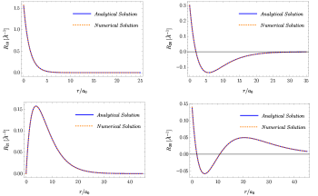
Figure 7: Comparison of numerical and analytical solutions for the Hydrogen radial wavefunctions $R_{10}$, $R_{20}$, $R_{21}$, and $R_{30}$, with $a_{0}$ the Bohr radius. We can see an excellent agreement between the two sets of wave functions, to the point that the overlaid plots are almost indistinguishable.

A.2 The interacting kernel for the Rytova-Keldysh potential

As in the Coulomb problem, it is also possible to obtain an analytical expression for the Hamiltonian and superposition kernels of the attractive Rytova-Keldysh potential. Obviously, the kinetic energy kernel and the superposition kernel are the same as those given in the previous section. The Rytova-Keldysh energy kernel is given by

$$K^{RK}(m,\zeta_{i},\zeta_{j})=\frac{e^{2}}{8r_{0}^{2}\epsilon_{0}}(\zeta_{i}+\zeta_{j})^{-|m|-3/2}\times$$

$$\left[-2\epsilon_{1}\Gamma\left(\frac{3}{2}+|m|\right){}_{2}F_{2}\left(1,\frac{3}{2}+|m|;\frac{3}{2},\frac{3}{2};-\frac{\epsilon_{1}}{4r_{0}^{2}(\zeta_{i}+\zeta_{j})}\right)\right.$$

$$\left.+\pi r_{0}\sqrt{\zeta_{i}+\zeta_{j}}G_{11}^{21}\bigg{(}\frac{\epsilon_{1}^{2}}{4r_{0}^{2}(\zeta_{i}+\zeta_{j})}\bigg{|}\begin{array}[]{c}{{-|m|;-1/2}}\\ {{0,0;-1/2}}\end{array}\bigg{)}\right]\,,$$ (53)

where ${}_{p}F_{q}$ is the generalized hypergeometric function, $G_{pq}^{mn}$ is the Meijer-G function, and $\epsilon_{1}$ is the average dielectric function of the substrate and capping layer.

References

References

- [1] Kenan P. Fears, Dmitri Y. Petrovykh, Sara J. Photiadis, and Thomas D. Clark, Circular Dichroism Analysis of Cyclic Helical Peptides Adsorbed on Planar Fused Quartz, Langmuir 29, 10095 (2013).
- [2] Eigil B. NielsenJohn A. Schellman, The absorption spectra of simple amides and peptides, J. Phys. Chem. 71, 2297 (1967).
- [3] Kimberly A. Bode and Jon Applequist, Improved Theoretical Absorption and Circular Dichroic Spectra of Helical Polypeptides Using New Polarizabilities of Atoms and NC’O Chromophores, J. Phys. Chem. 100, 17825 (1996).
- [4] Or Berger, Lihi Adler-Abramovich, Michal Levy-Sakin, Assaf Grunwald, Yael Liebes-Peer, Mor Bachar, Ludmila Buzhansky, Estelle Mossou, V. Trevor Forsyth, Tal Schwartz, Yuval Ebenstein, Felix Frolow, Linda J. W. Shimon, Fernando Patolsky, and Ehud Gazit, Light-emitting self-assembled peptide nucleic acids exhibit both stacking interactions and Watson?Crick base pairing, Nat. Nano. 10, 353 (2015).
- [5] Kenji Watanabe, Takashi Tanigushi, and Hisao Kanda, Direct-bandgap properties and evidence for ultraviolet lasing of hexagonal boron nitride single crystal, Nat. Mat. 3, 404 (2014).
- [6] B. Arnaud, S. Lebegue, P. Rabiller, and M. Alouani, Huge Excitonic Effects in Layered Hexagonal Boron Nitride, Phys. Rev. Lett. 96, 026402 (2006).
- [7] Andrea Marini, Ab Initio Finite-Temperature Excitons, Phs. Rev. Lett. 101, 106405 (2008).
- [8] Li Song, Lijie Ci, Hao Lu, Pavel B. Sorokin, Chuanhong Jin, Jie Ni, Alexander G. Kvashnin, Dmitry G. Kvashnin, Jun Lou, Boris I. Yakobson, and Pulickel M. Ajayan, Large Scale Growth and Characterization of Atomic Hexagonal Boron Nitride Layers, Nano Letters 10, 3209 (2010).
- [9] Yijing Stehle, Harry M. Meyer III, Raymond R. Unocic, Michelle Kidder, Georgios Polizos, Panos G. Datskos, Roderick Jackson, Sergei N. Smirnov, and Ivan V. Vlassiouk, Synthesis of Hexagonal Boron Nitride Monolayer: Control of Nucleation and Crystal Morphology, Chem. Matt. 27, 8041 (2015).
- [10] X. K. Cao, B. Clubine, J. H. Edgar, J. Y. Lin, and H. X. Jiang, Two-dimensional excitons in three-dimensional hexagonal boron nitride, App. Phys. Lett. 103, 191106 (2013).
- [11] G. Cassabois, P. Valvin, and B. Gil Hexagonal boron nitride is an indirect bandgap semiconductor, Nat. Phot. 10, 262 (2016).
- [12] Nikolai Dontschuk, Alastair Stacey, Anton Tadich, Kevin J. Rietwyk, Alex Schenk, Mark T. Edmonds, Olga Shimoni, Chris I. Pakes, Steven Prawer, and Jiri Cervenka, A graphene field-effect transistor as a molecule-specific probe of DNA nucleobases, Nat. Comm. 6, 6563 (2015).
- [13] Rui Campos, Jeroême Borme, Joana Rafaela Guerreiro, George Machado Jr., Maria Fátima Cerqueira, Dmitri Y. Petrovykh, and Pedro Alpuim, Attomolar Label-Free Detection of DNA Hybridization with Electrolyte-Gated Graphene Field-Effect Transistors, ACS Sens. 4, 286 (2019).
- [14] Gang Wang, Alexey Chernikov, Mikhail M. Glazov, Tony F. Heinz, Xavier Marie, Thierry Amand, and Bernhard Urbaszek, Colloquium: Excitons in atomically thin transition metal dichalcogenides, Rev. Mod. Phys. 90, 021001 (2018).
- [15] K. Zhang, Y. Feng, F. Wang, Z. Yang, and J. Wang, Two dimensional hexagonal boron nitride (2d-hbn): synthesis, properties and applications, Journal of Materials Chemistry C, vol. 5, 11992 (2017).
- [16] Xinsheng Wang, Mongur Hossain1, Zhongming Wei, and Liming Xie, Growth of two-dimensional materials on hexagonal boron nitride (h-BN), Nanotechnology 30, 034003 (2019).
- [17] Anshuman Kumar, Tony Low, Kin Hung Fung, Phaedon Avouris, and Nicholas X. Fang, Tunable Light–Matter Interaction and the Role of Hyperbolicity in Graphene–hBN System, Nano Lett. 15, 3172 (2015).
- [18] Peining Li, Martin Lewin, Andrey V. Kretinin, Joshua D. Caldwell, Kostya S. Novoselov, Takashi Taniguchi, Kenji Watanabe, Fabian Gaussmann, and Thomas Taubner, Hyperbolic phonon-polaritons in boron nitride for near-field optical imaging and focusing, Nat. Comm. 6, 7507 (2015).
- [19] Tony Low, Andrey Chaves, Joshua D. Caldwell, Anshuman Kumar, Nicholas X. Fang, Phaedon Avouris, Tony F. Heinz, Francisco Guinea, Luis Martin-Moreno, and Frank Koppens, Nat. Mat. 16, 182 (2017).
- [20] Hailin Xu, Xi Wang, Xing Jiang, Xiaoyu Daia, and Yuanjiang Xiang, Guiding characteristics of guided waves in slab waveguide with hexagonal boron nitride, J. App. Phys. 122, 033103 (2017).
- [21] S. Dai, Z. Fei, Q. Ma, A. S. Rodin, M. Wagner, A. S. McLeod, M. K. Liu, W. Gannett, W. Regan, K. Watanabe, T. Taniguchi, M. Thiemens, G. Dominguez, A. H. Castro Neto, A. Zettl, F. Keilmann, P. Jarillo-Herrero, M. M. Fogler, and D. N. Basov , Tunable Phonon Polaritons in Atomically Thin van der Waals Crystals of Boron Nitride, Science 343, 1125 (2014).
- [22] F. Ferreira, A. J. Chaves, N. M. R. Peres, and R. M. Ribeiro, Excitons in hexagonal boron nitride single-layer: a new platform for polaritonics in the ultraviolet, J. Opt. Soc. Am. 36, 674 (2019).
- [23] B. Hunt, J. D. Sanchez-Yamagishi, A. F. Young, M. Yankowitz, B. J. LeRoy, K. Watanabe, T. Taniguchi, P. Moon, M. Koshino, P. Jarillo-Herrero, and R. C. Ashoori, Massive Dirac Fermions and Hofstadter Butterfly in a van der Waals Heterostructure, Science 340, 1427 (2013).
- [24] A. J. Chaves, R. M. Ribeiro, T. Frederico, N. M. R. Peres, Excitonic effects in the optical properties of 2D materials: An equation of motion approach, 2D Materials 4, 025086 (2017).
- [25] N. S. Rytova, The Screened Potential of a Pont Charge in a Thin Film, Moscow University Physics Bulletin 22, 30 (1967).
- [26] L. V. Keldysh, Coulomb interaction in thin semiconductor and semimetal films, Soviet Journal of Experimental and Theoretical Physics Letters 29, 658 (1979).
- [27] J. J. Griffin and J. A. Wheeler, Motion in nuclei by the method of generator coordinates, Physical Review, 108, 311-327 (1957).
- [28] José Rachid Mohallem, A further study on the discretisation of the Griffin-Hill-Wheeler equation, Zeitschrift f\”ur Physik D 3, 339 (1986).
- [29] kash Laturia, Maarten L. Van de Put, and William G. Vandenberghe, Dielectric properties of hexagonal boron nitride and transition metal dichalcogenides: from monolayer to bulk, npj 2D Mater. Appl. 2, 6 (2018).
- [30] C. Elias, P. Valvin, T. Pelini, A. Summerfield, C.J. Mellor, T.S. Cheng, L. Eaves, C.T. Foxon, P.H. Beton, S.V. Novikov, B. Gil, and G. Cassabois, Direct band-gap crossover in epitaxial monolayer boron nitride, Nat. Comm. 10, 2639 (2019).
- [31] Léonard Schué, Ingrid Stenger, Frédéric Fossard, Annick Loiseau, and Julien Barjon, Characterization methods dedicated to nanometer-thick hBN layers, 2D Matt. 4, 015028 (2016).
- [32] Lu Hua Li and Ying Chen, Atomically Thin Boron Nitride: Unique Properties and Applications, Adv. Funct. Mater. 26, 2594 (2016).
- [33] K. T. Winther, K. S. Thygesen, Band structure engineering in van der waals heterostructures via dielectric screening: the gw method, 2D Materials 4, 025059 (2017).
- [34] T. Galvani, F. Paleari, H. P. Miranda, A. Molina-Sanchez, L. Wirtz, S. Latil, H. Amara, and F. Ducastelle, Excitons in boron nitride single layer, Phys. Rev. B 94, 125303 (2016).
- [35] K. Mengle and E. Kioupakis, Impact of the stacking sequence on the bandgap and luminescence properties of bulk, bilayer, and monolayer hexagonal boron nitride, APL Materials 7, 021106 (2019).
- [36] D. Wickramaratne, L. Weston, and C. G. Van de Walle, Monolayer to bulk properties of hexagonal boron nitride, The J. of Phys. Chem. C 122, 25 524-25 529 (2018).
- [37] I. Guilhon, M. Marques, L. K. Teles, M. Palummo, O. Pulci, Silvana Botti, and F. Bechstedt, Out-of-plane excitons in two-dimensional crystals, Phys. Rev. B 99, 161201(R) (2019).
- [38] Pierluigi Cudazzo, Ilya V. Tokatly, and Angel Rubio, Dielectric screening in two-dimensional insulators: Implications for excitonic and impurity states in graphane, Phys. Rev. B 84, 085406 (2011).
- [39] Mads L. Trolle, Thomas G. Pedersen, Valerie Véniard, Model dielectric function for 2D semiconductors including substrate screening, Sci. Rep. 7, 39844 (2017).
- [40] S. Latini, T. Olsen, K. S. Thygesen, Excitons in van der waals heterostructures: The important role of dielectric screening, Phys. Rev. B 92, 245123 (2015).
- [41] André Chaves, private communication.
- [42] E. I. Blount, Formalisms of band theory, Solid State Physics 13, 305 (1962).
- [43] G. B. Ventura, D. J. Passos, J. M. B. Lopes dos Santos, J. M. Viana Parente Lopes, and N. M. R. Peres, Gauge covariances and nonlinear optical responses, Phys. Rev. B 96, 035431 (2017).
- [44] Maurizia Palummo, Marco Bernardi, and Jeffrey C. Grossman, Exciton Radiative Lifetimes in Two-Dimensional Transition Metal Dichalcogenides, Nano Letters 15, 2794 (2015).
- [45] Giovanni Scuri, You Zhou, Alexander A. High, Dominik S. Wild, Chi Shu, Kristiaan De Greve, Luis A. Jauregui, Takashi Taniguchi, Kenji Watanabe, Philip Kim, Mikhail D. Lukin, and Hongkun Park Large Excitonic Reflectivity of Monolayer MoSe2 Encapsulated in Hexagonal Boron Nitride, Phys. Rev. Lett. 120, 037402 (2018).
- [46] Jonas S. Laursen, Jens Engel-Andreasen, and Christian A. Olsen, Peptoid Foldamers at Last, Acc. Chem. Res. 48, 2696 (2015).
- [47] F. Hipolito, Thomas G. Pedersen, and Vitor M. Pereira, Nonlinear photocurrents in two-dimensional systems based on graphene and boron nitride, Phys. Rev. B 94, 045434 (2016).
- [48] X. Yang, S. Guo, F. Chan, K. Wong, and W. Ching, Analytic solution of a two-dimensional hydrogen atom. i. nonrelativistic theory, Phys. Rev. A 43, 1186 (1991).