Astronomy Letters, 2019, Vol. 45, No 6, pp. 331–340.

Galactic Rotation Based on OB Stars from

the Gaia DR2 Catalogue

V.V. Bobylev and A.T. Bajkova

Pulkovo Astronomical Observatory, Russian Academy of Sciences,

Pulkovskoe sh. 65, St. Petersburg, 196140 Russia

Abstract—We have studied a sample containing $\sim\-6000$ OB stars with proper motions and trigonometric parallaxes from the Gaia DR2 catalogue. The following parameters of the angular velocity of Galactic rotation have been found: $\Omega_{0}=29.70\pm 0.11$ km s^-1 kpc^-1, $\Omega^{\prime}_{0}=-4.035\pm 0.031$ km s^-1 kpc^-2, and $\Omega^{\prime\prime}_{0}=0.620\pm 0.014$ km s^-1 kpc^-3. The circular rotation velocity of the solar neighborhood around the Galactic center is $V_{0}=238\pm 5$ km s^-1 for the adopted Galactocentric distance of the Sun $R_{0}=8.0\pm 0.15$ kpc. The amplitudes of the tangential and radial velocity perturbations produced by the spiral density wave are $f_{\theta}=4.4\pm 1.4$ km s^-1 and $f_{R}=5.1\pm 1.2$ km s^-1, respectively; the perturbation wavelengths are $\lambda_{\theta}=1.9\pm 0.5$ kpc and $\lambda_{R}=2.1\pm 0.5$ kpc for the adopted four-armed spiral pattern. The Sun’s phase in the spiral density wave is $\chi_{\odot}=-178^{\circ}\pm 12^{\circ}$.

INTRODUCTION

Stars of spectral types O and B are an important tool for studying the Galaxy and its subsystems. Being young, they trace well the spiral arms, because most of them have not receded very far (except for the small percentage of high-velocity runaway stars) from their birthplace. OB stars have nearly circular Galactic orbits and, therefore, serve as an excellent material for studying the Galactic rotation. They are visible from great distances and, therefore, are well suited for studying the Galactic disk structure, the spiral pattern, the central bar, young open star clusters, OB associations, and various star-forming regions. Such studies were performed, for example, by Y.M. Georgelin and Y.P. Georgelin (1976), Byl and Ovenden (1978), Maiz-Apellániz (2001), Zabolotskikh et al. (2002), and Russeil (2003).

At present, the Gaia space experiment (Brown et al. 2016) is a valuable data source for studying the structure and kinematics of the Galaxy. The Gaia second data release, Gaia DR2, was published in April 2018 (Brown et al. 2018; Lindegren et al. 2018). It contains the trigonometric parallaxes and proper motions of $\sim$1.3 billion stars. The mean trigonometric parallax errors lie in the range 0.02–0.04 mas for bright stars ($G<15^{m}$) and reach 0.7 mas for faint stars ($G=20^{m}$). For more than 7 million stars of spectral types F–G–K the line-of-sight velocities have been determined with a mean error of $\sim$1 km s^-1. The errors in the line-of-sight velocities of OB stars are known to be considerably larger due to the peculiarities of the spectra for these stars.

Highly accurate Gaia DR2 data have already yielded a number of significant kinematic results. For example, based on Gaia DR2 data, Helmi et al. (2018) determined new proper motions for 75 Galactic globular clusters and a number of dwarf galaxies that are Milky Way satellites, including the Magellanic Clouds. A new estimate of the Galactic mass, $9.8^{+6.7}_{-2.7}\times 10^{11}M_{\odot}$, was obtained by analyzing their space velocities. Based on a kinematic analysis of the space velocities from the Gaia DR2 catalogue, Antoja et al. (2018) detected some manifestations of the still ongoing wobble of the Milky Way disk after the passage of the Sagittarius dwarf galaxy through it.

Based on data from the Gaia DR2 catalogue, Cantat-Gaudin et al. (2018) determined new mean proper motions for 1229 open star clusters (OSCs), while for a significant fraction of this OSC list Soubiran et al. (2018) deduced the mean values of their line-of-sight velocities exclusively from Gaia DR2 data. The kinematics of these OSCs was studied by Bobylev and Bajkova (2019). The spatial and intrinsic kinematic properties of a number of young stellar associations close to the Sun have been studied with hitherto unprecedented detail (Zari et al. 2018; Franciosini et al. 2018; Roccatagliata et al. 2018; Kounkel et al. 2018).

A sample containing $\sim$500 OB stars with parallaxes and proper motions from the Gaia DR2 catalogue was studied by Bobylev and Bajkova (2018b). The goal of this paper is to improve the Galactic rotation parameters and the parameters of the Galactic spiral density wave based on a huge sample of OB stars for which the trigonometric parallaxes and proper motions are available in the Gaia DR2 catalogue. Such a sample of OB stars containing data on 5772 stars has recently been published by Xu et al. (2018).

METHOD

Galactic Rotation Parameters

We know three stellar velocity components from observations: the line-of-sight velocity $V_{r}$ and the two tangential velocity components $V_{l}=4.74r\mu_{l}\cos b$ and $V_{b}=4.74r\mu_{b}$ along the Galactic longitude $l$ and latitude $b,$ respectively, expressed in km s^-1. Here, the coefficient 4.74 is the ratio of the number of kilometers in an astronomical unit to the number of seconds in a tropical year, and $r=1/\pi$ is the stellar heliocentric distance in kpc that we calculate via the stellar parallax $\pi.$ The proper motion components $\mu_{l}\cos b$ and $\mu_{b}$ are expressed in mas yr^-1.

To determine the parameters of the Galactic rotation curve, we use the equations derived from Bottlinger’s formulas, in which the angular velocity $\Omega$ is expanded into a series to terms of the second order of smallness in $r/R_{0}$:

$$\begin{array}[]{lll}V_{r}=-U_{\odot}\cos b\cos l-V_{\odot}\cos b\sin l-W_{\odot}\sin b\\ +R_{0}(R-R_{0})\sin l\cos b\Omega^{\prime}_{0}+0.5R_{0}(R-R_{0})^{2}\sin l\cos b\Omega^{\prime\prime}_{0},\end{array}$$ (1)

$$\begin{array}[]{lll}V_{l}=U_{\odot}\sin l-V_{\odot}\cos l-r\Omega_{0}\cos b\\ +(R-R_{0})(R_{0}\cos l-r\cos b)\Omega^{\prime}_{0}+0.5(R-R_{0})^{2}(R_{0}\cos l-r\cos b)\Omega^{\prime\prime}_{0},\end{array}$$ (2)

where $R$ is the distance from the star to the Galactic rotation axis:

$$R^{2}=r^{2}\cos^{2}b-2R_{0}r\cos b\cos l+R^{2}_{0}.$$ (3)

The quantity $\Omega_{0}$ is the angular velocity of Galactic rotation at the solar distance $R_{0},$ the parameters $\Omega^{\prime}_{0}$ and $\Omega^{\prime\prime}_{0}$ are the corresponding derivatives of this angular velocity, and the linear rotation velocity of the Galaxy is $V_{0}=|R_{0}\Omega_{0}|.$ In Eqs. (1) and (2) the five unknowns $U_{\odot},V_{\odot},\Omega_{0},\Omega^{\prime}_{0}$ and $\Omega^{\prime\prime}_{0}$ are to be determined; in Eq. (1) there are only four unknown parameters, because the angular velocity of rotation $\Omega_{0}$ is absent.

Note a number of studies devoted to determining the mean distance from the Sun to the Galactic center using its individual determinations in the last decade by independent methods. For example, $R_{0}=8\pm 0.2$ kpc (Vallée 2017), $R_{0}=8.4\pm 0.4$ kpc (de Grijs and Bono 2017), or $R_{0}=8\pm 0.15$ kpc (Camarillo et al. 2018). Based on these reviews, here we adopted $R_{0}=8\pm 0.15$ kpc.

The kinematic parameters are determined by solving the conditional equations (1) and (2) by the least-squares method (LSM). We use weights of the form $w_{r}=S_{0}/\sqrt{S_{0}^{2}+\sigma^{2}_{V_{r}}}$ and $w_{l}=S_{0}/\sqrt{S_{0}^{2}+\sigma^{2}_{V_{l}}},$ where $S_{0}$ is the “cosmic” dispersion, $\sigma_{V_{r}}$ and $\sigma_{V_{l}}$ are the dispersions of the corresponding observed velocities. $S_{0}$ is comparable to the root-mean-square residual $\sigma_{0}$ (the error per unit weight) that is calculated when solving the conditional equations (1) and (2). In this paper we adopted $S_{0}=12$ km s^-1 typical for young stars. The system of equations (1) and (2) is solved in several iterations using the $3\sigma$ criterion to eliminate the stars with large residuals.

When the stars distributed uniformly over the celestial sphere are analyzed, a third equation, where the components $V_{b}$ are on the left-hand side, is also used. When analyzing the OB stars located virtually in the Galactic plane, where $\sin b\approx 0,$ using the equation with $V_{b}$ is ineffective. However, even when the system of conditional equations (1) and (2) is solved simultaneously, the velocity $W_{\odot}$ is determined poorly. Therefore, in this paper we assume it to be known, $W_{\odot}=7$ km s^-1.

Influence of the Spiral Density Wave

To study the influence of the Galactic spiral density wave, it is first necessary to calculate three space velocities $U,V,W$ for each star, where $U$ is directed from the Sun to the Galactic center, $V$ is in the direction of Galactic rotation, and $W$ is directed to the north Galactic pole. These velocities are calculated via the components $V_{r},$ $V_{l},$ and $V_{b}$:

$$\begin{array}[]{lll}U=V_{r}\cos l\cos b-V_{l}\sin l-V_{b}\cos l\sin b,\\ V=V_{r}\sin l\cos b+V_{l}\cos l-V_{b}\sin l\sin b,\\ W=V_{r}\sin b+V_{b}\cos b.\end{array}$$ (4)

Thus, they can be determined only for those stars for which both line-of-sight velocities and proper motions have been measured.

We can find two velocities, $V_{R}$ directed radially away from the Galactic center and the velocity $V_{circ}$ orthogonal to it pointing in the direction of Galactic rotation, based on the following relations:

$$\begin{array}[]{lll}V_{circ}=U\sin\theta+(V_{0}+V)\cos\theta,\\ V_{R}=-U\cos\theta+(V_{0}+V)\sin\theta,\end{array}$$ (5)

where the position angle $\theta$ obeys the relation $\tan\theta=y/(R_{0}-x)$, and $x,y,z$ are the rectangular heliocentric coordinates of the star (the velocities $U,V,W$ are directed along the corresponding $x,y,z$ axes), $V_{0}$ is the linear rotation velocity of the Galaxy at the solar distance $R_{0}.$ The velocities $V_{R}$ and $W$ are virtually independent of the pattern of the Galactic rotation curve. To analyze the periodicities in the tangential velocities, it is necessary to form the residual velocities $\Delta V_{circ}$ by taking into account a smoothed Galactic rotation curve.

According to the linear theory of density waves (Lin and Shu 1964), the influence of the spiral density wave is described by the following relations:

$$\begin{array}[]{lll}V_{R}=-f_{R}\cos\chi,\\ \Delta V_{circ}=f_{\theta}\sin\chi,\end{array}$$ (6)

where

$$\chi=m[\cot(i)\ln(R/R_{0})-\theta]+\chi_{\odot}$$ (7)

is the phase of the spiral density wave ($m$ is the number of spiral arms, $i$ is the pitch angle of the spiral pattern, and $\chi_{\odot}$ is the Sun’s radial phase in the spiral density wave); $f_{R}$ and $f_{\theta}$ are the amplitudes of the radial and tangential velocity perturbations, which are assumed to be positive. As an analysis of the present day highly accurate data showed, the periodicities associated with the spiral density wave also manifest themselves in the vertical velocities $W$ (Bobylev and Bajkova 2015; Rastorguev et al. 2017).

We apply a modified spectral analysis (Bajkova and Bobylev 2012) to study the periodicities in the velocities $V_{R}$ and $\Delta V_{circ}$. The wavelength $\lambda$ (the distance between adjacent spiral arm segments measured along the radial direction) is calculated from the relation

$$\lambda m\cot(i)=2\pi R_{0}.$$ (8)

Let there be a series of measured velocities $V_{R_{n}}$ (these can be both radial ($V_{R}$) and tangential ($\Delta V_{circ}$) velocities), $n=1,\dots,N$, where $N$ is the number of objects. The objective of our spectral analysis is to extract a periodicity from the data series in accordance with the adopted model describing a spiral density wave with parameters $f,$ $\lambda$ (or $i)$ and $\chi_{\odot}$.

Having taken into account the logarithmic behavior of the spiral density wave and the position angles of the objects $\theta_{n}$, our spectral (periodogram) analysis of the series of velocity perturbations is reduced to calculating the square of the amplitude (power spectrum) of the standard Fourier transform (Bajkova and Bobylev 2012):

$$\bar{V}_{\lambda_{k}}=\frac{1}{N}\sum_{n=1}^{N}V^{{}^{\prime}}_{n}(R^{{}^{\prime}}_{n})\exp\biggl{(}-j\frac{2\pi R^{{}^{\prime}}_{n}}{\lambda_{k}}\biggr{)},$$ (9)

where $\bar{V}_{\lambda_{k}}$ is the $k$th harmonic of the Fourier transform with wavelength $\lambda_{k}=D/k$, $D$ is the period of the series being analyzed,

$$\begin{array}[]{lll}R^{{}^{\prime}}_{n}=R_{0}\ln(R_{n}/R_{0}),\\ V^{{}^{\prime}}_{n}(R^{{}^{\prime}}_{n})=V_{n}(R^{{}^{\prime}}_{n})\times\exp(jm\theta_{n}).\end{array}$$ (10)

The sought-for wavelength $\lambda$ corresponds to the peak value of the power spectrum $S_{peak}$. The pitch angle of the spiral density wave is derived from Eq. (8). The pitch angle of the spiral density wave is derived from Eq. (9). We determine the perturbation amplitude and phase by fitting the harmonic with the wavelength found to the observational data. The following relation can also be used to estimate the perturbation amplitude:

$$f_{R}(f_{\theta})=2\times\sqrt{S_{peak}}.$$ (11)

Thus, our approach consists of two steps: (i) the construction of a smooth Galactic rotation curve and (ii) a spectral analysis of the radial ($V_{R}$) and residual tangential ($\Delta V_{circ}$) velocities. This method was applied by Bobylev and Bajkova (2012, 2018b) to study the kinematics of young Galactic objects.

Monte Carlo Simulations

We use Monte Carlo simulations to estimate the errors in the parameters of the spiral density wave being determined. In accordance with this method, we generate $M$ independent realizations of data on the parallaxes and velocities of objects with their random measurement errors that are known to us.

We assume that the measurement errors of the data are distributed normally with a mean equal to the nominal value and a dispersion equal to $\sigma_{l}={error}_{l},l=1,\dots,N_{d}$, where $N_{d}$ is the number of data and $error_{l}$ denotes the measurement error of a single measurement with number $l$ (one sigma). Each element of a random realization is formed independently by adding the nominal value of the measured data with number $l$ and the random number generated according to a normal law with zero mean and dispersion $\sigma_{l}$. Note that the latter is limited from above by $3\sigma_{l}$.

Each random realization of data with number $j$ ($j=1,\dots,M$) generated in this way is then processed according to the algorithm described above to determine the sought-for parameters $f_{R}^{j},\lambda^{j},$ and $\chi_{\odot}^{j}$. The mean values of the parameters and their dispersions are then determined from the derived sequences of estimates: $m_{f_{R}}\pm\sigma_{f_{R}},m_{\lambda}\pm\sigma_{\lambda},m_{\chi_{\odot}}\pm\sigma_{\chi_{\odot}}$. The statistical parameters of the spiral density wave pitch angle $i$ can be determined using Eq. (8): $m_{i}\pm\sigma_{i}$.

DATA

In this paper we use the catalogue of OB stars produced by Xu et al. (2018). It gives the proper motions and trigonometric parallaxes taken from the Gaia DR2 catalogue for 5772 stars of spectral types O–B2. For $\sim$2000 OB stars it gives the line-of-sight velocities taken from the SIMBAD electronic database. Note that in the catalogue by Xu et al. (2018) the line-of-sight velocities of OB stars are given relative to the local standard of rest and, therefore, we convert them to the heliocentric ones in advance using the parameters of the standard solar apex $(U,V,W)_{\odot}=(10.3,15.3,7.7)$ km s^-1.

Correction to the Gaia DR2 Parallaxes

The presence of a possible systematic offset $\Delta\pi=-0.029$ mas in the Gaia DR2 parallaxes with respect to an inertial reference frame was first pointed out by Lindegren et al. (2018). Here, the minus means that this correction should be added to the Gaia DR2 stellar parallaxes to reduce them to the standard.

Arenou et al. (2018) provided an overview of the results of comparing the Gaia DR2 parallaxes with 29 independent distance scales that confirm the presence of an offset in the Gaia DR2 parallaxes $\Delta\pi\sim-0.03$ mas. The discrepancies between individual results turned out to be very large (stars of the Hipparcos and RECONS programs, stars of the dwarf galaxies Phoenix, Leo I, and Leo II); as a result, Arenou et al. (2018) did not deduce the mean value for this correction. Subsequently, some of the results used by Arenou et al. (2018) were confirmed by other authors based on new data. For example, based on RR Lyrae stars, Muraveva et al. (2018) found the correction $\Delta\pi=-0.057$ mas, or based on 88 radio stars whose trigonometric parallaxes were measured by various authors by means of VLBI, Bobylev (2019) obtained an estimate of $\Delta\pi=-0.038\pm 0.046$ mas.

Completely new results are of greatest interest. Stassun and Torres (2018) found the correction $\Delta\pi=-0.082\pm 0.033$ mas by comparing the parallaxes of 89 detached eclipsing binaries with their trigonometric parallaxes from the Gaia DR2 catalogue. These stars were selected from published data using very rigorous criteria imposed on the photometric parameters. As a result, the relative errors in the stellar radii, effective temperatures, and bolometric luminosities, from which the distances are estimated, do not exceed 3%.

By comparing the Gaia DR2 trigonometric parallaxes and photometric parallaxes of 94 OSCs, Yalyalieva et al. (2018) found the correction $\Delta\pi=-0.045\pm 0.009$ mas. The high accuracy of this estimate is attributable to the high accuracy of the photometric distance estimates for OSCs obtained by invoking first-class infrared photometric surveys, such as IPHAS, 2MASS, WISE, and Pan-STARRS.

Riess et al. (2018) obtained an estimate of $\Delta\pi=-0.046\pm 0.013$ mas based on a sample of 50 long period Cepheids when comparing their parallaxes with those from the Gaia DR2 catalogue. The photometric parameters of these Cepheids measured from the Hubble Space Telescope were used.

By comparing the distances of $\sim$3000 stars from the APOKAS-2 catalogue (Pinsonneault et al. 2018) belonging to the red giant branch with the Gaia DR2 data, Zinn et al. (2018) found the correction $\Delta\pi=-0.053\pm 0.003$ mas. These authors also obtained a close value, $\Delta\pi=-0.050\pm 0.004$ mas, by analyzing stars belonging to the red giant clump. The distances to such stars were estimated from asteroseismic data. According to these authors, the parallax errors here are approximately equal to the errors in estimating the stellar radius and are, on average, 1.5%. Such small errors in combination with the enormous number of stars allowed $\Delta\pi$ to be determined with a high accuracy.

The listed results lead to the conclusion that the trigonometric parallaxes of stars from the Gaia DR2 catalogue should be corrected by applying a small correction. We will be oriented to the results of Yalyalieva et al. (2018), Riess et al. (2018), and Zinn et al. (2018), which look most reliable.

Table 1: The Galactic rotation parameters found from OB stars with proper motions and trigonometric parallaxes ($\sigma_{\pi}/\pi<15\%$) for various corrections to the Gaia DR2 parallaxes

Parameters	$\pi=\pi+0$ mas	$\pi=\pi+0.02$ mas	$\pi=\pi+0.03$ mas	$\pi=\pi+0.05$ mas
$U_{\odot},$ km s-1	$9.49\pm 0.72$	$9.19\pm 0.71$	$9.24\pm 0.70$	$9.27\pm 0.69$
$V_{\odot},$ km s-1	$12.59\pm 0.69$	$13.16\pm 0.68$	$12.81\pm 0.69$	$13.24\pm 0.67$
$\Omega^{{}^{\prime}}_{0},$ km s-1 kpc-2	$-3.380\pm 0.100$	$-3.559\pm 0.098$	$-3.591\pm 0.097$	$-3.811\pm 0.096$
$\Omega^{{}^{\prime\prime}}_{0},$ km s-1 kpc-3	$0.483\pm 0.118$	$0.676\pm 0.014$	$0.613\pm 0.125$	$0.742\pm 0.120$
$\sigma_{0},$ km s-1	18.32	18.35	18.54	18.54
$N_{\star}$	1783	1839	1876	1925
$U_{\odot},$ km s-1	$6.12\pm 0.26$	$6.25\pm 0.25$	$6.22\pm 0.24$	$6.17\pm 0.23$
$V_{\odot},$ km s-1	$6.77\pm 0.44$	$7.10\pm 0.42$	$7.13\pm 0.40$	$7.38\pm 0.38$
$\Omega_{0},$ km s-1 kpc-1	$29.90\pm 0.13$	$29.76\pm 0.13$	$29.73\pm 0.13$	$29.56\pm 0.12$
$\Omega^{{}^{\prime}}_{0},$ km s-1 kpc-2	$-4.202\pm 0.037$	$-4.175\pm 0.036$	$-4.154\pm 0.035$	$-4.119\pm 0.035$
$\Omega^{{}^{\prime\prime}}_{0},$ km s-1 kpc-3	$0.647\pm 0.032$	$0.658\pm 0.032$	$0.645\pm 0.029$	$0.648\pm 0.029$
$\sigma_{0},$ km s-1	12.17	11.84	11.73	11.31
$N_{\star}$	4249	4408	4488	4620
$(\Omega^{{}^{\prime}}_{0})_{V_{r}}/(\Omega^{{}^{\prime}}_{0})_{V_{l}}$	0.80	0.85	0.86	0.93

The results obtained only from the line-of-sight velocities $V_{r}$ (Eq. (1)) and only from the component $V_{l}$ (Eq. (2)) are given in the upper and lower parts, respectively. $N_{\star}$ is the number of stars used.

Table 2: The Galactic rotation parameters found from OB stars with proper motions and trigonometric parallaxes when simultaneously solving Eqs. (1) and (2) for various constraints on the relative errors of the parallaxes from the Gaia DR2 catalogue; the correction $\Delta\pi=0.050$ mas was added to the parallaxes of OB stars

Parameters	$\sigma_{\pi}/\pi<10\%$	$\sigma_{\pi}/\pi<15\%$	$\sigma_{\pi}/\pi<20\%$	$\sigma_{\pi}/\pi<30\%$
$U_{\odot},$ km s-1	$6.13\pm 0.26$	$6.48\pm 0.24$	$6.61\pm 0.23$	$6.62\pm 0.23$
$V_{\odot},$ km s-1	$10.20\pm 0.38$	$9.95\pm 0.33$	$9.79\pm 0.31$	$8.99\pm 0.28$
$\Omega_{0},$ km s-1 kpc-1	$29.09\pm 0.17$	$29.13\pm 0.13$	$29.03\pm 0.13$	$29.15\pm 0.13$
$\Omega^{{}^{\prime}}_{0},$ km s-1 kpc-2	$-4.161\pm 0.045$	$-4.058\pm 0.035$	$-3.992\pm 0.033$	$-3.915\pm 0.032$
$\Omega^{{}^{\prime\prime}}_{0},$ km s-1 kpc-3	$0.824\pm 0.055$	$0.767\pm 0.030$	$0.742\pm 0.023$	$0.620\pm 0.015$
$\sigma_{0},$ km s-1	12.84	13.54	13.93	14.28
$N_{\star}$	3313	4569	4959	5175
$A,$ km s-1 kpc-1	$16.64\pm 0.18$	$16.23\pm 0.14$	$15.97\pm 0.13$	$15.66\pm 0.13$
$B,$ km s-1 kpc-1	$-12.45\pm 0.24$	$-12.89\pm 0.19$	$-13.06\pm 0.18$	$-13.50\pm 0.18$
$V_{0},$ km s-1	$232.8\pm 4.6$	$233.0\pm 4.5$	$232.3\pm 4.5$	$233.2\pm 4.5$

$N_{\star}$ is the number of stars used.

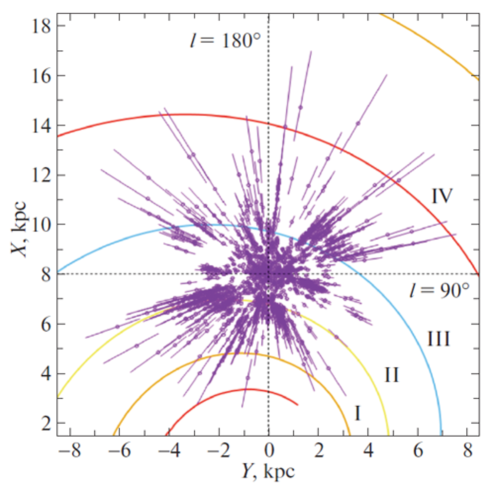
Figure 1: (Color online) Distribution of the sample of OB stars for which both line-of-sight velocities and proper motions are available on the $XY$ plane; the Sun has coordinates $(X,Y)=(8,0)$ kpc, the four-armed spiral pattern with a pitch angle of $-13^{\circ}$ is shown (Bobylev and Bajkova 2014), the spiral arm segments are numbered by Roman numerals.

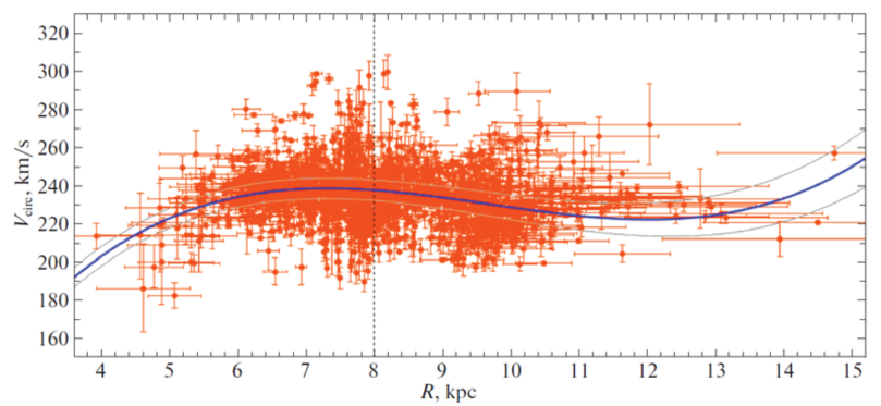
Figure 2: (Color online) Circular velocities of OB stars versus Galactocentric distance, the Galactic rotation curve constructed according to the solution (12) with the $1\sigma$ boundaries of the confidence intervals; the vertical dashed line marks the Sun’s position.

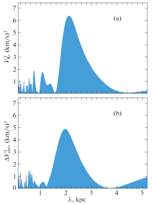
Figure 3: (Color online) Power spectra for the radial (a) and residual tangential (b) velocities of OB stars.

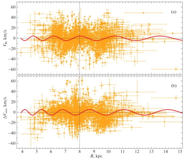
Figure 4: (Color online) Radial (a) and residual tangential (b) velocities of OB stars versus Galactocentric distance; the vertical dashed line marks the Sun’s position.

RESULTS

The Entire Sample of OB Stars

Let us first consider all our OB stars for various constraints on the relative trigonometric parallax errors and various corrections of the zero point of the Gaia DR2 parallaxes, $\Delta\pi$.

Table 1 gives the kinematic parameters obtained for various corrections to the Gaia DR2 parallaxes as a result of the separate solutions of Eqs. (1) and (2). We used OB stars with relative trigonometric parallax errors less than 15%. As can be seen from the table, there is a noticeable influence of the correction $\Delta\pi$ when the kinematic parameters are determined using the line-of-sight velocities of stars (the upper part of Table 1). The second derivative of the angular velocity of Galactic rotation $\Omega^{{}^{\prime\prime}}_{0}.$ is affected most strongly here.

The last row in Table 1 gives the ratio of the first derivative of the angular velocity found using only the line-of-sight velocities $(\Omega^{{}^{\prime}}_{0})_{V_{r}}$ to the one found using only the proper motions $(\Omega^{{}^{\prime}}_{0})_{V_{l}}$.

This method is based on the fact that the estimate of the first derivative of the angular velocity obtained from the proper motions depends very weakly on the error of the adopted distance scale, while the estimate of the first derivative of the angular velocity obtained from the line-of-sight velocities is inversely proportional to the adopted scale of the distance scale. Therefore, comparing the values of $\Omega_{0}^{\prime}$ found by various methods allows the correction factor of the distance scale $p$ to be found (Zabolotskikh et al. 2002; Rastorguev et al. 2017); in our case, $p=(\Omega^{{}^{\prime}}_{0})_{V_{r}}/(\Omega^{{}^{\prime}}_{0})_{V_{l}}$. The error in $p$ was calculated based on the relation $\sigma^{2}_{p}=(\sigma_{\Omega^{\prime}_{0V_{r}}}/\Omega^{\prime}_{0V_{l}})^{2}+(\Omega^{\prime}_{0V_{r}}\cdot\sigma_{\Omega^{\prime}_{0V_{l}}}/\Omega^{\prime 2}_{0V_{l}})^{2}.$ Having analyzed more than 50 000 stars from the TGAS catalogue (Brown et al. 2016), Bobylev and Bajkova (2018a) obtained an estimate of $p=0.97\pm 0.04.$ by this method. According to the results in Table 1, we can see that the distance scale factor $p$ tends to unity as the correction $\Delta\pi$ increases. On the other hand, the noticeable deviations of this factor from unity in the first columns of the table are determined almost entirely by $\Omega^{\prime}_{0V_{r}}$. It can be concluded that the quality of the line-of-sight velocities for this sample of OB stars is low.

Table 2 gives the kinematic parameters found when simultaneously solving the system of equations (1) and (2) for various constraints on the relative errors of the parallaxes from the Gaia DR2 catalogue. Here, the correction $\Delta\pi=0.050$ mas was added to the parallaxes of OB stars. The simultaneous solution is as follows. The OB stars with proper motions, line-of-sight velocities, and distances give two equations, (1) and (2), while the stars for which only the proper motions are available give only Eq. (2). As can be seen from Table 1, the stars with line-of-sight velocities are approximately half those with proper motions.

Based on a sample of 5335 stars, to the parallaxes of which we added the correction $\Delta\pi=0.050$ mas, we found the following kinematic parameters from the solution of only Eq. (2):

$$\begin{array}[]{lll}(U_{\odot},V_{\odot})=(6.53,7.27)\pm(0.24,0.31)~{}\hbox{km s${}^{-1}$},\\ \Omega_{0}=~{}29.70\pm 0.11~{}\hbox{km s${}^{-1}$ kpc${}^{-1}$},\\ \Omega^{{}^{\prime}}_{0}=-4.035\pm 0.031~{}\hbox{km s${}^{-1}$ kpc${}^{-2}$},\\ \Omega^{{}^{\prime\prime}}_{0}=~{}0.620\pm 0.014~{}\hbox{km s${}^{-1}$ kpc${}^{-3}$},\end{array}$$ (12)

where the error per unit weight is $\sigma_{0}=12.33$ km s^-1, the Oort constants are $A=16.14\pm 0.13$ km s^-1 kpc^-1 and $B=-13.56\pm 0.17$ km s^-1 kpc^-1, and the linear rotation velocity of the Galaxy at the solar distance is $V_{0}=237.6\pm 4.5$ km s^-1.

The parameters (12) should be compared with those given in the last column of Table 2, because both these solutions were obtained for identical constraints. Such a comparison shows that in the case where only the proper motions of OB stars (solution (12)) are used, the kinematic parameters are determined with smaller errors compared to the results of the simultaneous solution (Table 2).

OB Stars with Line-of-Sight Velocities

In this section we analyze the OB stars for which complete information is available. Thus, there are measurements of their trigonometric parallaxes, proper motions, and line-of-sight velocities. Such a sample contains more than 2000 OB stars. For each such star we can calculate the velocities $U,V,W$ as well as $V_{R}$ and $V_{circ}.$ The results of our analysis of these stars are presented in Figs. 1–4.

Previously (Tables 1 and 2), Eqs. (1) and (2)were solved in several iterations using the $3\sigma$ criterion to eliminate the stars with large residuals. Now, when selecting the OB stars, we use the following additional constraints to improve the quality of the space velocities (due to the low quality of the series of line-of-sight velocities for our OB stars):

$$\begin{array}[]{lll}\sqrt{U^{2}+V^{2}+W^{2}}<60~{}\hbox{km s${}^{-1}$},\\ \qquad|W|<40~{}\hbox{km s${}^{-1}$},\end{array}$$ (13)

where the rotation curve (12) was taken into account when calculating the velocities $U,V,$ and $W.$

Figure 1 shows the distribution of 2023 OB stars with relative parallax errors no more than 30% on the Galactic $XY$ plane. The distances to them were calculated by applying the correction $\Delta\pi=0.050$ mas to the original trigonometric parallaxes. The Roman numerals in the figure number the following spiral arm segments: Scutum (I), Carina–Sagittarius (II), Perseus (III), and the Outer Arm (IV).

Figure 2 plots the circular velocities of 2023 OB stars against the Galactocentric distance and presents the Galactic rotation curve constructed according to the solution (12).

Based on the deviation from the Galactic rotation curve (12), we calculated the residual circular velocities $\Delta V_{circ}$ for this sample of OB stars. Next, based on the series of their radial ($V_{R}$) and residual tangential ($\Delta V_{circ}$) velocities, we found the parameters of the Galactic spiral density wave by applying a periodogram analysis.

Figure 3 shows the power spectra for the velocities of OB stars. It is clearly seen from this figure that the peaks of the distribution lie almost at the same $\lambda$. Indeed, the perturbation wavelengths are $\lambda_{R}=2.1\pm 0.5$ kpc (for checking, we calculate the pitch angle $i=-9\pm 2^{\circ}$ for the adopted four-armed spiral pattern, $m=4,$ from Eq. (8)) and $\lambda_{\theta}=1.9\pm 0.5$ kpc ($i=-9\pm 2^{\circ}$). The amplitudes of the radial and tangential velocity perturbations are $f_{R}=5.1\pm 1.2$ km s^-1 and $f_{\theta}=4.4\pm 1.4$ km s^-1, respectively.

Figure 4 presents the radial and residual tangential velocities of OB stars. The corresponding periodic curves constructed with the parameters found as a result of our spectral analysis are shown. It is clearly seen that these curves, in Figs. 4a and 4b, run with a phase shift of approximately $90^{\circ}$. We measure the Sun’s phase in the spiral density wave $\chi_{\odot}$ from the Carina-Sagittarius arm ($R\sim 7$ kpc); in our case, its value turned out to be $-178\pm 12^{\circ}$.

DISCUSSION

Based on 130 masers with measured VLBI trigonometric parallaxes, Rastorguev et al. (2017) found the solar velocity components $(U_{\odot},V_{\odot})=(11.40,17.23)\pm(1.33,1.09)$ km s^-1 and the following parameters of the Galactic rotation curve: $\Omega_{0}=28.93\pm 0.53$ km s^-1 kpc^-1, $\Omega^{{}^{\prime}}_{0}=-3.96\pm 0.07$ km s^-1 kpc^-2, $\Omega^{{}^{\prime\prime}}_{0}=0.87\pm 0.03$ km s^-1 kpc^-3, and $V_{0}=243\pm 10$ km s^-1 (for $R_{0}=8.40\pm 0.12$ kpc found).

Based on a sample of 495 OB stars with proper motions from the Gaia DR2 catalogue, Bobylev and Bajkova (2018b) found the following kinematic parameters: $(U,V,W)_{\odot}=(8.16,11.19,8.55)\pm(0.48,0.56,0.48)$ km s^-1, $\Omega_{0}=28.92\pm 0.39$ km s^-1 kpc^-1, $\Omega^{{}^{\prime}}_{0}=-4.087\pm 0.083$ km s^-1 kpc^-2 and $\Omega^{{}^{\prime\prime}}_{0}=0.703\pm 0.067$ km s^-1 kpc^-3, where $V_{0}=231\pm 5$ km s^-1 (for the adopted $R_{0}=8.0\pm 0.15$ kpc). Note that when seeking the solution (12), in this paper we used an order of magnitude more OB stars.

Here, we have excellent agreement in the parameters found, with the errors of the parameters being determined in the solution (12) being very small. In this sense, the solution (12) presently gives estimates of the parameters $\Omega_{0},$ $\Omega^{{}^{\prime}}_{0}$ and $\Omega^{{}^{\prime\prime}}_{0}$ that are among the best ones.

Note also the parameters found by Bobylev and Bajkova (2019) based on a sample of 326 young ($logt<8$) OSCs with proper motions and distances from the Gaia DR2 catalogue: $(U,V,W)_{\odot}=(8.53,11.22,7.83)\pm(0.38,0.46,0.32)$ km s^-1, $\Omega_{0}=28.71\pm 0.22$ km s^-1 kpc^-1, $\Omega^{{}^{\prime}}_{0}=-4.100\pm 0.058$ km s^-1 kpc^-2 and $\Omega^{{}^{\prime\prime}}_{0}=0.736\pm 0.033$ km s^-1 kpc^-3.

Parameters of the spiral density wave. The mean pitch angle of the global four-armed spiral pattern in our Galaxy $i=-13.6\pm 0.4^{\circ}$. is given in the review of Vallée (1917b). Then, at $m=4$ and $R_{0}=8$ kpc $\lambda=3$ kpc follows from Eq. (8). It can be seen that an analysis of our sample of OB stars gives a smaller $\lambda$ and, accordingly, a smaller pitch angle $|i|:9^{\circ}-10^{\circ}$.

Having analyzed the spatial distribution of a large sample of classical Cepheids, Dambis et al. (2015) estimated the pitch angle of the spiral pattern, $i=-9.5^{\circ}\pm 0.1^{\circ}$, and the Sun’s phase, $\chi_{\odot}=-121^{\circ}\pm 3^{\circ}$, for the four-armed spiral pattern.

On the other hand, having analyzed maser sources with VLBI parallaxes, Rastorguev et al. (2017) found $i=-10.4^{\circ}\pm 0.3^{\circ}$ and $\chi_{\odot}=-125^{\circ}\pm 10^{\circ},$ which is in good agreement with our results.

According to the model estimates by Burton (1971), the amplitudes of the velocity perturbations from a density wave ($f_{R},f_{\theta}$) depend on R. Both these velocity perturbations have a fairly broad maximum in the region $0.5R_{0}<R<0.9R_{0}$, reaching $\approx 8$ km s^-1 ($f_{R}$ is everywhere larger than $f_{\theta}$ by $\approx 1$ km s^-1); the velocity perturbations are about 4 km s^-1 near $0.2R_{0}$ and decrease to 2.5 km s^-1 in the vicinity of $1.3R_{0}.$

An analysis of the present-day data shows that in a wide vicinity of $R_{0},$ $f_{R}$ and $f_{\theta}$ are typically 4–9 km s^-1 from masers (Rastorguev et al. 2017), OB stars (Bobylev and Bajkova 2018b), or Cepheids (Bobylev and Bajkova 2012). Note also the new values of $f_{R}=4.6\pm 0.7$ km s^-1 and $f_{\theta}=1.1\pm 0.4$ km s^-1 obtained recently by Loktin and Popova (2019) from an analysis of the present-day data on OSCs. The perturbation amplitudes found in this paper, particularly $f_{R},$ are in good agreement with the results listed above.

When OB stars, young OSCs, or young Cepheids are analyzed, the absolute value of the phase lies within the range $100-140^{\circ}$. As we see, the Sun’s phase in the spiral density wave $-178\pm 12^{\circ}$ found by us differs noticeably from the listed results of other authors that were obtained by analyzing young objects.

CONCLUSIONS

We studied the kinematic properties of a large sample of OB stars ($\sim$6000 stars) with proper motions and trigonometric parallaxes from the GaiaDR2 catalogue and partly also with their line-of-sight velocities ($\sim$2000 stars). For this purpose, we used the catalogue of OB stars produced by Xu et al. (2018).

We analyzed the separate and simultaneous solutions of the basic kinematic equations for various constraints on the relative trigonometric parallax errors and various corrections of the zero point of the Gaia DR2 parallaxes, $\Delta\pi$. As a result, we showed that in the solar neighborhood under consideration (with a radius of about 4 kpc) the parameters of the smooth Galactic rotation curve are determined more accurately in the solution where only the proper motions of OB stars are used (solution (12)), which was obtained with the involvement of 5335 OB stars. We showed that there is a noticeable influence of the correction $\Delta\pi$ when determining the kinematic parameters in the case where the line-of-sight velocities of OB stars are used. $\Omega^{{}^{\prime\prime}}_{0}$ is affected most strongly here.

To study the influence of the Galactic spiral density wave, we used a sample of 2023 OB stars with relative parallax errors no more than 30% as well as with known line-of-sight velocities and proper motions. The amplitudes of the tangential and radial velocity perturbations produced by the spiral density wave are $f_{\theta}=4.4\pm 1.4$ km s^-1 and $f_{R}=5.1\pm 1.2$ km s^-1, respectively; the perturbation wavelengths are $\lambda_{\theta}=1.9\pm 0.5$ kpc and $\lambda_{R}=2.1\pm 0.5$ kpc for the adopted four-armed spiral pattern. The Sun’s phase in the spiral density wave was found to be $\chi_{\odot}=-178^{\circ}\pm 12^{\circ}$.

FUNDING

This work was supported in part by the Basic Research Program no. 12 of the Presidium of the Russian Academy of Sciences, the “Cosmos: Studies of Fundamental Processes and Their Interrelations” Subprogram.

REFERENCES

1. T. Antoja, A. Helmi, M. Romero-Gómez, D. Katz, C. Babusiaux, R. Drimmel, D. W. Evans, F. Figueras, et al., Nature (London, U.K.) 561, 360 (2018).

2. F. Arenou, X. Luri, C. Babusiaux, C. Fabricius, A. Helmi, T. Muraveva, A. C. Robin, F. Spoto, et al. (Gaia Collab.), Astron. Astrophys. 616, 17 (2018).

3. A. T. Bajkova and V. V. Bobylev, Astron. Lett. 38, 549 (2012).

4. V. V. Bobylev and A. T. Bajkova, Mon. Not. R. Astron. Soc. 437, 1549 (2014).

5. V. V. Bobylev and A. T. Bajkova, Mon. Not. R. Astron. Soc. 447, L50 (2015).

6. V. V. Bobylev and A. T. Bajkova, Astron. Lett. 44, 184 (2018a).

7. V. V. Bobylev and A. T. Bajkova, Astron. Lett. 44, 675 (2018b).

8. V. V. Bobylev, Astron. Lett. 45, 10 (2019).

9. V. V. Bobylev and A. T. Bajkova, Astron. Lett. 45, 109 (2019).

10. A. G. A. Brown, A. Vallenari, T. Prusti, J. de Bruijne, F. Mignard, R. Drimmel, et al. (Gaia Collab.), Astron. Astrophys. 595, 2 (2016).

11. A. G. A. Brown, A. Vallenari, T. Prusti, J. de Bruijne, C. Babusiaux, C. A. L. Bailer-Jones, M. Biermann, D. W. Evans, et al. (Gaia Collab.), Astron. Astrophys. 616, 1 (2018).

12. W. B. Burton, Astron. Astrophys. 10, 76 (1971).

13. J. Byl and M. W. Ovenden, Astrophys. J. 225, 496 (1978).

14. T. Camarillo, M. Varun, M. Tyler, and R. Bharat, Publ. Astron. Soc. Pacif. 130, 4101 (2018).

15. T. Cantat-Gaudin, C. Jordi, A. Vallenari, A. Bragaglia, L. Balaguer-Nuńéz, C. Soubiran, et al., Astron. Astrophys. 618, 93 (2018).

16. A. K. Dambis, L. N. Berdnikov, Yu. N. Efremov, A. Yu. Knyazev, A. S. Rastorguev, E. V. Glushkova, V. V. Kravtsov, D. G. Turner, D. J. Majaess, and R. Sefako, Astron. Lett. 41, 489 (2015).

17. E. Franciosini, G. G. Sacco, R. D. Jeffries, F. Damiani, V. Roccatagliata, D. Fedele, and S. Randich, Astron. Astrophys. 616, 12 (2018).

18. Y. M. Georgelin and Y. P. Georgelin, Astron. Astrophys. 49, 57 (1976).

19. R. de Grijs and G. Bono, Astrophys. J. Suppl. Ser. 232, 22 (2017).

20. A. Helmi, F. van Leeuwen, P. J. McMillan, D. Massari, T. Antoja, A. C. Robin, L. Lindegren, U. Bastian, et al. (Gaia Collab.), Astron. Astrophys. 616, 12 (2018).

21. M. Kounkel, K. Covey, G. Suárez, C. Román-Zuńiga, J. Hernandez, K. Stassun, K. O. Jaehnig, E. D. Feigelson, et al., Astron. J. 156, 84 (2018).

22. C. C. Lin and F. H. Shu, Astrophys. J. 140, 646 (1964).

23. L. Lindegren, J. Hernandez, A. Bombrun, S. Klioner, U. Bastian, M. Ramos-Lerate, A. de Torres, H. Steidelmuller, et al. (Gaia Collab.), Astron. Astrophys. 616, 2 (2018).

24. A. V. Loktin and M. E. Popova, Astrophys. Bull. 74 (2019, in press).

25. J. Maiz-Apellaniz, Astron. J. 121, 2737 (2001).

26. T. Muraveva, H. E. Delgado, G. Clementini, L. M. Sarro, and A. Garofalo, Mon. Not. R. Astron. Soc. 481, 1195 (2018).

27. M. H. Pinsonneault, Y. P. Elsworth, J. Tayar, A. Serenelli, D. Stello, J. Zinn, S. Mathur, R. Garcia, et al., Astrophys. J. Suppl. Ser. 239, 32 (2018).

28. A. S. Rastorguev, M. V. Zabolotskikh, A. K. Dambis, N. D. Utkin, V. V. Bobylev, and A. T. Bajkova, Astrophys. Bull. 72, 122 (2017).

29. A. G. Riess, S. Casertano, W. Yuan, L. Macri, B. Bucciarelli, M. G. Lattanzi, J. W. MacKenty, J. B. Bowers, et al., Astrophys. J. 861, 126 (2018).

30. V. Roccatagliata, G. G. Sacco, E. Franciosini, and S. Randich, Astron. Astrophys. 617, L4 (2018).

31. D. Russeil, Astron. Astrophys. 397, 133 (2003).

32. C. Soubiran, T. Cantat-Gaudin, M. Romero-Gomez, L. Casamiquela, C. Jordi, A. Vallenari, T. Antoja, L. Balaguer-Nuńez, et al., Astron. Astrophys. 619, 155 (2018).

33. K. G. Stassun and G. Torres, Astrophys. J. 862, 61 (2018).

34. J. P. Vallée, Astrophys. Space Sci. 362, 79 (2017a).

35. J. P. Vallée, New Astron. Rev. 79, 49 (2017b).

36. Y. Xu, S. B. Bian, M. J. Reid, J. J. Li, B. Zhang, Q. Z. Yan, T. M. Dame, K. M. Menten, et al., Astron. Astrophys. 616, L15 (2018).

37. L. N. Yalyalieva, A. A. Chemel’, E. V. Glushkova, A. K. Dambis, and A. D. Klinichev, Astrophys. Bull. 73, 335 (2018).

38. M. V. Zabolotskikh, A. S. Rastorguev, and A. K. Dambis, Astron. Lett. 28, 454 (2002).

39. E. Zari, H. Hashemi, A. G. A. Brown, K. Jardine, and P. T. de Zeeuw, Astron. Astrophys. 620, 172 (2018).

40. J. C. Zinn, M. H. Pinsonneault, D. Huber, and D. Stello, arXiv: 1805.02650 (2018).