Evidence for Low Radiative Efficiency or Highly Obscured Growth of $z>7$ Quasars

Abstract

The supermassive black holes (SMBHs) observed at the centers of all massive galaxies are believed to have grown via luminous accretion during quasar phases in the distant past. The fraction of inflowing rest mass energy emitted as light, the radiative efficiency, has been inferred to be 10%, in agreement with expectations from thin disk accretion models. But the existence of billion solar-mass SMBHs powering quasars at $z>7$ challenges this picture: provided they respect the Eddington limit, there is not enough time to grow $z>7$ SMBHs from stellar remnant seeds unless the radiative efficiency is below 10%. Here we show that one can constrain the radiative efficiencies of the most distant quasars known using foreground neutral intergalactic gas as a cosmological-scale ionizing photon counter. From the Ly$\alpha$ absorption profiles of ULAS J1120+0641 ($z=7.09$) and ULAS J1342+0928 ($z=7.54$), we determine posterior median radiative efficiencies of 0.08% and 0.1%, respectively, and the combination of the two measurements rule out the canonical 10% efficiency at 99.8% credibility after marginalizing over the unknown obscured fraction. This low radiative efficiency implies rapid mass accretion for the earliest SMBHs, greatly easing the tension between the age of the Universe and the SMBH masses. However, our measured efficiency may instead reflect nearly complete obscuration by dusty gas in the quasar host galaxies over the vast majority of their SMBH growth. Assuming 10% efficiency during unobscured phases, we find that the obscured fraction would be $>82\%$ at 95% credibility, and imply a $25.7^{+49.6}_{-16.5}$ times larger obscured than unobscured luminous quasar population at $z>7$.

1 Introduction

The quasar phenomenon has been studied for more than 50 years (Schmidt, 1963). Quasar central engines are believed to be accretion disks feeding material onto supermassive black holes (Rees, 1984). In the standard picture of SMBH growth, the rest mass energy of accreted mass is divided between radiation and black hole mass growth via the radiative efficiency $\epsilon$, implying that emission of quasar light is concomitant with black hole growth. In the local Universe, dormant supermassive black holes reside at the centers of all massive galaxies, and galaxies with more stellar mass in a spheroidal bulge host more massive black holes (Ferrarese & Merritt, 2000; Gebhardt et al., 2000). The connection between distant quasar “progenitors” and “relic” supermassive black holes is encapsulated in the Soltan argument, which states that the integrated emission from quasars over cosmic time is proportional to the total mass in supermassive black holes today via the radiative efficiency (Soltan, 1982),

$$\rho_{\rm BH}(z=0)=\int_{0}^{\infty}\frac{dt}{dz}dz\int_{L_{\rm min}}^{\infty}\frac{1-\epsilon}{\epsilon}\frac{L_{\rm q}}{c^{2}}\Phi(L,z)dL,$$ (1)

where $\Phi(L,z)$ is the quasar luminosity function in some observed band and $L_{\rm q}$ represents the bolometric luminosity of a quasar with observed luminosity $L$. It then follows that the radiative efficiency can be inferred by commensurating the energy density of quasar light with the inferred mass density of supermassive black holes in the local Universe. Applications of this argument by various groups have measured radiative efficiencies of $\approx 10\%$ (e.g. Yu & Tremaine 2002; Shankar et al. 2009; Ueda et al. 2014) after statistically correcting for the obscured quasar population, consistent with predictions of analytic thin disk accretion models in general relativity (e.g. Thorne 1974). However, current understanding is that these thin disk models represent an idealization as they fail to reproduce quasar spectral energy distributions (e.g. Koratkar & Blaes 1999). Numerical simulations of quasar accretion disks reveal a more complex picture of geometrically thick disks supported by radiation pressure, within which a substantial fraction of the radiation can be advected into the central black hole, potentially dramatically lowering the radiative efficiency (e.g. Sa̧dowski et al. 2014).

The bolometric luminosity of a quasar accretion disk is typically written as

$$L_{\rm bol}=\epsilon\dot{M}c^{2}=\frac{\epsilon}{1-\epsilon}\dot{M}_{\rm BH}c^{2},$$ (2)

where $\dot{M}$ is the total mass inflow rate and $\dot{M_{\rm BH}}$ is the growth rate of the black hole. The maximum luminosity of a quasar can be estimated by equating the gravitational acceleration from the black hole with radiation pressure on electrons in the infalling gas, known as the Eddington luminosity,

$$L_{\rm edd}=\frac{4\pi GM_{\rm BH}cm_{\rm p}}{\sigma_{\rm T}}.$$ (3)

From equation (2), the characteristic timescale for growing a black hole at the Eddington limit, the Salpeter time $t_{\rm S}$, is then

$$t_{\rm S}=\frac{1-\epsilon}{\epsilon}\frac{4\pi Gm_{\rm p}}{c\sigma_{\rm T}}\approx 45\,{\rm Myr}\times\frac{(1-\epsilon)/\epsilon}{9}.$$ (4)

Assuming a fixed Eddington ratio $L/L_{\rm Edd}$, a black hole with seed mass $M_{\rm seed}$ at time $t_{\rm seed}$ will then grow as

$$M_{\rm BH}(t)=M_{\rm seed}e^{(L/L_{\rm Edd})([t-t_{\rm seed}]/t_{\rm S})}.$$ (5)

A lower radiative efficiency would decrease $t_{\rm S}$, and thus could alleviate the tension with growing supermassive black holes at the highest redshifts.

Luminous quasars with $\gtrsim 10^{9}$ $M_{\odot}$ black holes have been discovered at $z>7$ when the Universe was less than 800 Myr old (Mortlock et al., 2011; Bañados et al., 2018; Yang et al., 2018; Wang et al., 2018). Growing the observed $10^{9}$ $M_{\odot}$ black holes at $z\gtrsim 7$ from a $100$ $M_{\odot}$ initial seed requires $\approx 16$ e-foldings, which for $\epsilon=0.1$ corresponds to continuous Eddington-limited accretion for roughly the entire age of the Universe at that time. It seems implausible that these black holes have been growing since the Big Bang. However, demanding a later formation epoch, consistent with expectations for the death of the first stars in primordial galaxies at $z\sim 20$–$50$ (e.g. Tegmark et al. 1997), implies seeds in excess of $1000$ $M_{\odot}$ (Mazzucchelli et al., 2017; Bañados et al., 2018) which are then inconsistent with being stellar remnants (Heger et al., 2003).

Two classes of models have been proposed to resolve this tension. In the first, the black holes grow faster, either by explicitly violating the Eddington luminosity limit (e.g. Volonteri & Rees 2005) or by accreting at a much lower radiative efficiency (e.g. Madau et al. 2014). In the second, the initial seeds were much more massive than stellar remnants, either by forming monolithically via direct collapse of primordial gas (e.g. Bromm & Loeb 2003) or by coalescence of a dense Population III stellar cluster (e.g. Omukai et al. 2008). A method to directly measure the radiative efficiency of the highest redshift quasars would shed light on this tension and distinguish between these models. Indeed, the radiative efficiency inferred from the Soltan argument is both indirect and has negligible contribution from the rare $z>7$ quasar population.

The highest redshift quasars known reside within the “epoch of reionization,” when the first stars, galaxies, and accreting black holes ionized the hydrogen and helium in the Universe for the first time after cosmological recombination (Loeb & Furlanetto, 2013; Dayal & Ferrara, 2018). During reionization, abundant neutral hydrogen in the intergalactic medium (IGM) is expected to imprint two distinct Ly$\alpha$ absorption features on the rest-frame ultraviolet (UV) spectra of quasars. First, the “proximity zone” of enhanced Ly$\alpha$ transmission resulting from the quasar’s own ionizing radiation will be truncated by neutral hydrogen along our line-of-sight (Cen & Haiman, 2000). Second, a damping wing signature redward of rest-frame Ly$\alpha$ will be present, arising from the Lorentzian wings of the Ly$\alpha$ resonant absorption cross-section (Miralda-Escudé, 1998). The two highest redshift quasars known, ULAS J1120+0641 (Mortlock et al., 2011) (henceforth J1120+0641) at $z=7.09$, and ULAS J1342+0928 (Bañados et al., 2018) (henceforth J1342+0928) at $z=7.54$, both exhibit truncated proximity zones (Bolton et al., 2011; Davies et al., 2018b) (compared to similarly-luminous quasars at $z\sim 6$–$6.5$, Eilers et al. 2017) and show strong evidence for damping wing absorption (Mortlock et al., 2011; Bolton et al., 2011; Greig et al., 2017; Bañados et al., 2018; Davies et al., 2018b). As we show below, an extension of the Soltan argument to individual quasars is uniquely possible at $z\gtrsim 7$ due to the presence of neutral hydrogen in the IGM along our line of sight to the quasar.

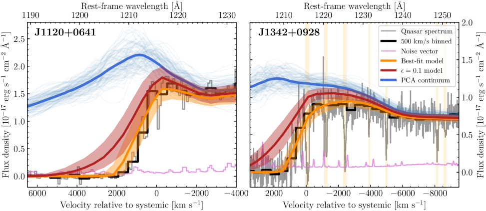
Figure 1: Quasar spectra and model fits close to rest-frame Ly$\alpha$. The grey and pink curves show the observed spectra and corresponding $1\sigma$ noise for J1120+0641 (left, VLT/FORS2, Mortlock et al. 2011) and J1342+0928 (right, Magellan/FIRE, Bañados et al. 2018). The black curves show the 500 km/s binned spectra used in our statistical analysis. The vertical shaded bands correspond to foreground metal absorption systems which were masked prior to binning. The thick blue curves show the PCA models for the intrinsic quasar spectra, while the thin blue curves show 100 draws from the distribution of covariant prediction uncertainty. The orange curves show the best-fit mean absorption models, corresponding to ($\langle x_{\rm HI}\rangle$, $N_{\rm ion}$) = (0.65, $1.2\times 10^{71}$) for J1120+0641 and ($\langle x_{\rm HI}\rangle$, $N_{\rm ion}$) = (0.90, $7.0\times 10^{70}$) for J1342+0928. The red curves show models assuming a fully neutral Universe ($\langle x_{\rm HI}\rangle=1$) and $N_{\rm ion}=5.7\times 10^{72}$ and $1.8\times 10^{72}$ for J1120+0641 and J1342+0928, respectively, corresponding to the maximum Ly$\alpha$ absorption with $N_{\rm ion}$ from equation (7) assuming $\epsilon=0.1$. The shaded regions around the orange and red curves correspond to the central 68% scatter of forward modeled mock spectra.

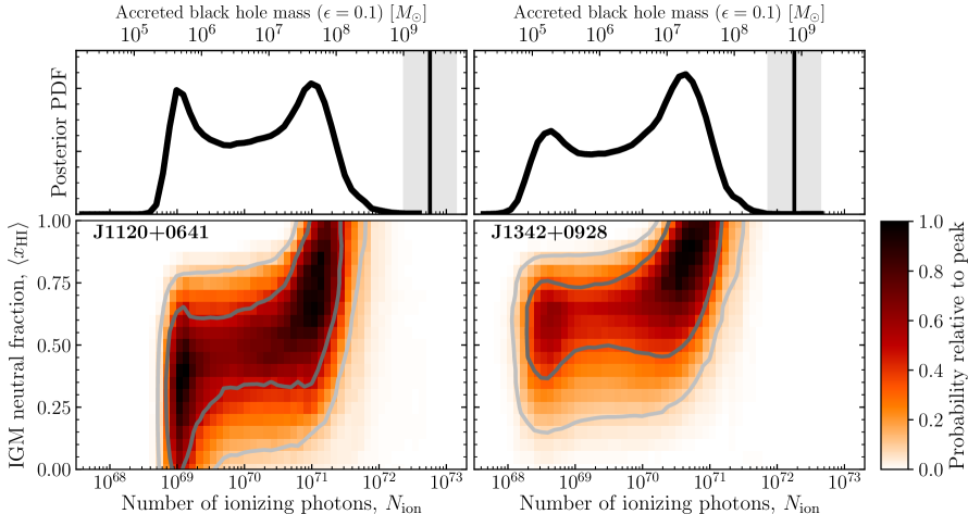
Figure 2: Joint posterior PDF of IGM neutral fraction and number of emitted ionizing photons. The lower panels show the two-dimensional posterior PDFs of $\langle x_{\rm HI}\rangle$ and $N_{\rm ion}$ inferred from the spectra of J1120+0641 (left) and J1342+0928 (right). The inner and outer grey contours enclose the central 68% and 95% probability, respectively. The top panels show the corresponding marginalized posterior PDFs for $N_{\rm ion}$. The vertical lines in the top panels indicate the expected $N_{\rm ion}$ from equation (7), assuming $\epsilon=0.1$ and the measured black hole masses of J1120+0641 ($M_{\rm BH}=2.47\times 10^{9}$ $M_{\odot}$) and J1342+0928 ($M_{\rm BH}=7.8\times 10^{8}$ $M_{\odot}$), with a shaded region indicating a $1\sigma$ systematic uncertainty of 0.4 dex in the mass measurements.

2 The Local Reionization Soltan Argument

The simple form of our analogy to the Soltan argument is as follows. The imprint of the neutral IGM on a reionization-epoch quasar spectrum constrains the total number of ionizing photons that the quasar ever emitted, $N_{\rm ion}$, which is proportional to the total accreted black hole mass, $\Delta M_{\rm BH}$, via the radiative efficiency $\epsilon$. From measurements of $N_{\rm ion}$ and $M_{\rm BH}$, we can thus constrain the average radiative efficiency during the entire growth history of the central SMBH. Below we explain this argument in more detail.

The total number of ionizing photons emitted by a quasar can be written as $N_{\rm ion}=\int\dot{N}_{\rm ion}(t)dt$, where $\dot{N}_{\rm ion}(t)$ is the quasar’s ionizing photon emission rate. Assuming unobscured emission along our line of sight, a constant bolometric correction $L_{\rm bol}=C_{\rm ion}\dot{N}_{\rm ion}$, and a constant radiative efficiency $\epsilon$, we can write

$$N_{\rm ion}=\int\frac{L_{\rm bol}(t)}{C_{\rm ion}}dt=\frac{\epsilon}{1-\epsilon}\frac{c^{2}}{C_{\rm ion}}\int\dot{M}_{\rm BH}(t)dt\propto\Delta M_{\rm BH}.$$ (6)

That is, given a bolometric correction and radiative efficiency, we can translate the number of ionizing photons into the mass growth of the black hole, $\Delta M_{\rm BH}\propto N_{\rm ion}$.

We assume the luminosity-dependent bolometric correction from $M_{1450}$ given in Table 3 of Runnoe et al. (2012), and convert from $M_{1450}$ to ionizing luminosity following the Lusso et al. (2015) spectral energy distribution (SED), resulting in $C_{\rm ion}=8.63\times 10^{-11}$ erg per ionizing photon. In the following, we neglect the uncertainty in this conversion because the uncertainty in the quasar SED is substantially smaller than the systematic uncertainty in the black hole mass. For J1120+0641 and J1342+0928, we compute ionizing photon emission rates of $\dot{N}_{\rm ion}^{\rm J1120}=1.2\times 10^{57}$ s^-1 and $\dot{N}_{\rm ion}^{\rm J1342}=1.4\times 10^{57}$ s^-1, and bolometric luminosities of $L_{\rm bol}^{\rm J1120}=2.7\times 10^{13}$ $L_{\odot}$ and $L_{\rm bol}^{\rm J1342}=3.1\times 10^{13}$ $L_{\odot}$, respectively.

Similar to analyses of the original Soltan argument, the census of ionizing photons recorded by the surrounding IGM must be modified to account for obscured phases when ionizing photons are absorbed before escaping the quasar host. That is, any ionizing photons emitted by the quasar which did not reach the IGM along our particular line of sight will be absent from our accounting of $N_{\rm ion}$ from the spectrum. Accordingly, we predict that black hole mass, radiative efficiency, and the number of ionizing photons should obey

$$\Delta M_{\rm BH}=10^{9}\,M_{\odot}\times\left(1-f_{\rm obsc}\right)^{-1}\left(\frac{(1-\epsilon)/\epsilon}{9}\right)\left(\frac{N_{\rm ion}}{2.3\times 10^{72}}\right),$$ (7)

where $f_{\rm obsc}$ is the fraction of emitted ionizing photons that never reached the IGM along our line of sight. This “local reionization Soltan argument” thus enables one to constrain the radiative efficiency of an individual quasar via its spectrum close to rest-frame Ly$\alpha$.

3 Constraints on the Radiative Efficiency of $z>7$ Quasars

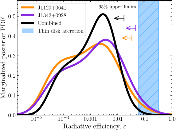
Figure 3: Marginalized posterior PDF of the radiative efficiency $\epsilon$. The orange and purple curves show the posterior PDFs of $\epsilon$ for J1120+0641 and J1342+0928, respectively, marginalized over obscuration and the systematic uncertainty in their black hole masses. The black curve shows the combined constraint under the assumption that both quasars have the same true radiative efficiency. Arrows indicate 95% credibility upper limits on $\epsilon$. The blue shaded region shows the range of radiative efficiencies predicted for thin accretion disks in general relativity (Thorne, 1974).

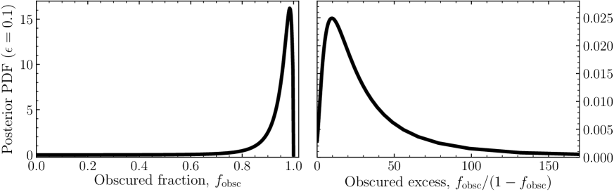
Figure 4: Constraints on the obscuration of $z>7$ quasars assuming $\epsilon=0.1$. Left: Posterior PDF for $f_{\rm obsc}$, combining the constraints from J1120+0641 and J1342+0928. Right: Combined posterior PDF for the relative number of obscured versus unobscured quasars, $f_{\rm obsc}/(1-f_{\rm obsc})$.

We measured $N_{\rm ion}$ for the two highest redshift quasars known, J1120+0641 and J1342+0928, by analyzing the Ly$\alpha$ absorption in their rest-frame UV spectra in a very similar fashion to Davies et al. (2018b). The intrinsic, unabsorbed quasar spectrum close to rest-frame Ly$\alpha$ was estimated via a predictive principal component analysis (PCA) approach from Davies et al. (2018a). In Figure 1 we show the two quasar spectra close to rest-frame Ly$\alpha$ (grey and black curves) compared to their respective PCA continuum models (blue curves). Both quasars show compelling evidence for an IGM damping wing and truncated proximity zones, as previously shown by Davies et al. (2018b).

We model reionization-epoch quasar spectra via a multi-scale approach following Davies et al. (2018b) (see also Appendix A). The large-scale topology of reionization around massive dark matter halos was computed in a (400 Mpc)³ volume using a modified version of the 21cmFAST code (Mesinger et al. 2011; Davies & Furlanetto, in prep.), and we stitched lines of sight through this ionization field onto skewers of baryon density fluctuations from a separate (100 Mpc$/h)^{3}$ Nyx hydrodynamical simulation (Lukić et al., 2015). Finally, we performed 1D ionizing radiative transfer to model the ionization and heating of the IGM by the quasar (Davies et al., 2016, 2019).

Through a Bayesian analysis on a grid of forward-modeled mock Ly$\alpha$ spectra from our simulations (Appendix A), we jointly constrained the total number of ionizing photons emitted by the quasars ($N_{\rm ion}$) and the volume-averaged neutral fraction of the IGM ($\langle x_{\rm HI}\rangle$). The mean Ly$\alpha$ absorption profiles of our best-fit models and their 68% scatter in the mock spectra are shown as the orange curves and shaded regions in Figure 1. The red curves in Figure 1 show alternative models where the IGM is fully neutral and $N_{\rm ion}$ for each quasar is instead determined via equation (7), assuming $\epsilon=0.1$, $f_{\rm obsc}=0$, and $\Delta M_{\rm BH}=M_{\rm BH}$. These curves thus correspond to the maximum Ly$\alpha$ absorption in the standard view of UV-luminous radiatively efficient SMBH growth. The canonical radiative efficiency appears to be highly inconsistent with the data.

More quantitatively, in the bottom panels of Figure 2 we show the joint posterior probability distribution functions (PDFs) for $N_{\rm ion}$ and $\langle x_{\rm HI}\rangle$ from our analysis of J1120+0641 (left) and J1342+0928 (right). In the top panels of Figure 2 we show the marginalized posterior PDFs for $N_{\rm ion}$. Through the lens of equation (7), we can view these marginalized posterior PDFs as constraints on the total accreted black hole mass, indicated by the upper axes, where we assume $\epsilon=0.1$. The vertical lines show the measured black holes masses for J1120+0641 and J1342+0928, with shaded regions indicating their systematic uncertainty. For both quasars the inferred accreted mass is in strong disagreement with the measured black hole mass, or equivalently, a radiative efficiency much lower than 10% is required to match the observations.

At face value, the results above indicate a serious inconsistency between standard thinking about the radiative efficiency – informed by general relativity, accretion disk models, and the Soltan argument – and our measurements for these two reionization-epoch quasars. How can we reconcile the smaller than expected number of ionizing photons emitted towards Earth with the observed black hole masses? One possibility is that the bulk of the black hole growth resulted in fewer ionizing photons escaping into the IGM toward our line-of-sight due to obscuration by gas and dust in the quasar host galaxy (e.g. Hopkins et al. 2005). If the black holes grew appreciably during obscured phases, then this is clearly degenerate with $N_{\rm ion}$ as indicated in equation (7). Observations of similarly luminous quasars at lower redshifts $z\gtrsim 2$ find that $\sim 50\%$ of them are obscured (Polletta et al., 2008; Merloni et al., 2014), with some indication for increased obscuration at higher redshifts (Vito et al. 2018, see also Trebitsch et al. 2019).

To quantitatively constrain the radiative efficiency, accounting for both the degeneracy with obscuration and uncertainties in the black hole masses, we re-map our 1D constraint on $N_{\rm ion}$ (i.e. the upper panels of Figure 2) to a 3D space of radiative efficiency, black hole mass, and the obscured fraction (see Appendix B). Marginalizing the 3D distributions over obscuration (assuming a uniform linear prior from 0 to 100%) and black hole mass uncertainty (lognormal prior with $\sigma=0.4$ dex, Shen 2013) yields posterior PDFs for the radiative efficiency as shown in Figure 3. The posterior median radiative efficiencies of J1120+0641 and J1342+0928 are 0.08% and 0.1%, respectively, and the canonical 10% is ruled out at greater than 98 per cent probability by each quasar. The combined posterior PDF for both quasars, assuming both quasars have the same true radiative efficiency, is shown by the black curve in Figure 3, which is inconsistent with $\epsilon=0.1$ at 99.8 per cent probability.

We can also assess what an assumed radiative efficiency of $10\%$ would imply for the obscuration of $z>7$ quasars. The left panel of Figure 4 shows the combined posterior PDF of $f_{\rm obsc}$ from both quasars assuming $\epsilon=0.1$, implying $f_{\rm obsc}>82\%$ at 95% credibility. Such a high obscured fraction implies that there are many more similarly-luminous obscured quasars at $z>7$ which have not yet been identified. The right panel of Figure 4 shows the posterior PDF for the ratio of obscured to unobscured quasars, $f_{\rm obsc}/(1-f_{\rm obsc})$, which we computed from the $f_{\rm obsc}$ posterior PDF by a probability transformation. We constrain this ratio to be $25.7^{+49.6}_{-16.5}$ (posterior median and 68% credible interval), with a 95% credible lower limit of $4.4$.

4 Discussion & Conclusion

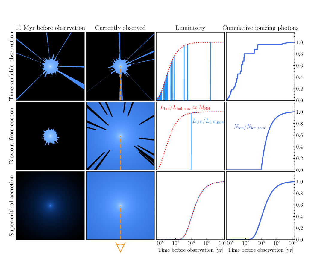
Figure 5: Possible solutions to the measured ionizing photon deficiency. The first two columns show schematic representations of the immediate environment of the $z>7$ quasars suggested by the measured deficit of ionizing photons. The blue regions are illuminated by the quasar while the black regions are not. The line of sight towards Earth is in the negative vertical direction as indicated by the orange dashed line. The leftmost column shows the quasar environment as it was 10 Myr ago, while the next column shows the quasar as it is observed today. The third column shows the UV (blue) and bolometric (red) luminosity history of the quasar, where we assume that the bolometric luminosity is proportional to the Eddington luminosity and thus its evolution indicates the growth of the black hole. The rightmost column shows the integrated number of ionizing photons that escaped into the IGM along our line of sight. The top and middle rows show two possible obscuration scenarios – time-variable obscuration with a large covering fraction (top), or full obscuration followed by blowout (middle). The bottom row shows the case where the radiative efficiency is low, leading to rapid black hole growth and a much less luminous quasar 10 Myr ago.

If this radiatively inefficient mode of growth that we have uncovered applies to quasars at later cosmic epochs, the Soltan argument implies previous analyses have underestimated the present day SMBH mass density by at least an order of magnitude. Without invoking extra SMBH mass locally, the only solution is that $z\gtrsim 7$ quasars grow or emit their radiation qualitatively differently from their lower redshift counterparts. A few possibilities are illustrated in Figure 5. It could be that $z>7$ quasar accretion disks are actually radiatively efficient with $\epsilon\simeq 0.1$ but simply have much more obscuration than inferred from studies of quasar demographics at lower redshift (see also Comastri et al. 2015). As our analysis only constrains the integrated number of ionizing photons emitted in our direction, it is agnostic to the exact nature of the obscuration. It could have been highly time-variable with obscured phases lasting $\gtrsim 10$ times longer than UV luminous ones (top row of Figure 5), or the black hole could have grown while fully enshrouded until a “blowout” event $\sim 1$ Myr ago when it transitioned to a UV luminous phase (middle row of Figure 5) (Hopkins et al., 2005). Either of these obscuration scenarios predicts many of comparably-luminous obscured quasars for every UV luminous one at $z>7$, as discussed above (Figure 4). The obscured fraction would then have to evolve very rapidly to avoid overproducing luminous obscured quasars at later times. Nevertheless, if such a population exists at $z>7$, future mid-IR observations with JWST have the potential to uncover them.

Finally, let us not exclude the possibility that $z>7$ quasar accretion disks are truly radiatively inefficient (bottom row of Figure 5). This would allow for rapid super-critical mass accretion rates with e-folding timescales much shorter than 45 Myr without violating the Eddington limit (equation 4), and has the appeal that it would easily explain the existence of $\gtrsim 10^{9}$ SMBHs at early cosmic times $z>7$ without requiring overly massive seeds. This last scenario poses an intriguing question: if the radiative efficiencies of the highest redshift quasars are radically different from those at lower redshift, why do their spectra appear nearly identical over eight decades in frequency (Bañados et al., 2015; Shen et al., 2018; Nanni et al., 2017)? Similar to the original Soltan argument, the radiative efficiency that we have derived is a luminosity-weighted average over the growth of the SMBH, which may differ from the efficiency of the currently observed accretion flow. Past phases of extremely super-critical accretion cannot be ruled out, provided that they only occur at $z>7$ – in the same vein, however, neither can exotic formation scenarios, e.g. direct collapse to $10^{9}M_{\odot}$, as long as they do not liberate UV photons. Future analyses of additional reionization-epoch quasars, combined with analogous measurements of the impact of luminous quasars on the IGM at lower redshifts (Eilers et al., 2018; Schmidt et al., 2018; Khrykin et al., 2019; Davies, 2019), will thus greatly improve our understanding of how SMBHs grew.

Appendix A Jointly Constraining the IGM H I Fraction and $N_{\rm ion}$

Here we summarize our methods for determining the intrinsic quasar continuum (Davies et al., 2018a) and Bayesian statistical analysis of reionization-epoch quasar transmission spectra (Davies et al., 2018b). We refer the reader to Davies et al. (2018a) and Davies et al. (2018b) for further details on the methods employed.

A.1 PCA Continuum Model

We predict the Mortlock et al. (2011) Gemini/GNIRS spectrum of J1120+0641 and the Bañados et al. (2018) Magellan/FIRE+Gemini/GNIRS spectrum of J1342+0928 identically to Davies et al. (2018a). The intrinsic quasar continuum in the Ly$\alpha$ region (the “blue side” of the spectrum, $\lambda_{\rm rest}=1180$–$1280$ Å) was estimated via a principal component analysis (PCA) method built from a training set of $12764$ quasar spectra from SDSS/BOSS [refs] queried from the IGMSpec spectral database (Prochaska, 2017). The red side of the quasar spectrum ($\lambda_{\rm rest}=1280$–$2850$ Å) was fit to a linear combination of red-side basis spectra, and the best-fit coefficients were “projected” to coefficients of blue-side basis spectra to predict the shape of the blue-side quasar spectrum. While the systemic redshifts of J1120+0641 ($z=7.0851$; Venemans et al. 2016) and J1342+0928 ($z=7.5413$; Venemans et al. 2017) are very well known, the systemic redshifts of the training set quasars are considerably uncertain. We thus defined a standardized “PCA redshift” frame by fitting the red-side coefficients simultaneously with a template redshift, and perform this same procedure when fitting the continua of the $z>7$ quasars.

As shown in Davies et al. (2018a), the continuum uncertainty varies depending on the spectral properties of the quasar in question. We thus determined custom covariant uncertainty in the modeled continua by testing the procedure on $127$ SDSS/BOSS quasars with the most similar red-side spectra to each $z>7$ quasar.

A.2 Grid of Ly$\alpha$ Transmission Spectra

Our numerical modeling of Ly$\alpha$ absorption in quasar spectra is identical to Davies et al. (2018b), as described in § 3, however we re-computed the simulations from Davies et al. (2018b) with a factor of five better sampling of quasar ages $t_{\rm q}$ to more carefully constrain $N_{\rm ion}\propto t_{\rm q}$. We computed 2400 radiative transfer simulations for each IGM neutral fraction $\langle x_{\rm HI}\rangle$ in steps of $\Delta x=0.05$ from 0 to 1.0, with Ly$\alpha$ transmission spectra computed for $t_{\rm q}$ separated by $\Delta\log{t_{\rm q}}=0.1$ from $10^{3}$ to $10^{8}$ years. We later translated these quasar ages into $N_{\rm ion}$ by multiplying by the current ionizing photon output $\dot{N}_{\rm ion}$ for each quasar.

A.3 Bayesian Statistical Method

Following Davies et al. (2018b), we performed a Bayesian statistical analysis by mapping out the likelihood function for summary statistics derived from forward-modeled mock data. We first bin the mock spectra to 500 km/s pixels, and fit 3 component Gaussian mixture models (GMM) to the flux distribution of each pixel for every pair of model parameter values $\theta=(\langle x_{\rm HI}\rangle,t_{\rm q})$ in our $21\times 51$ model grid. We define a pseudo-likelihood,

$$\tilde{L}({\theta})=\prod_{i}P_{{\rm GMM},i}(F_{i}|\theta),$$ (A1)

where $P_{{\rm GMM},i}(F_{i}|\theta)$ is the GMM of the $i$th pixel evaluated at its measured flux $F_{i}$ for model parameters $\theta$.

Treating the maximum pseudo-likelihood pair of parameter values $\theta_{\rm M\tilde{L}E}$ as a summary statistic to reduce the dimensionality of our data, we computed the posterior PDF of $\theta$ via Bayes’ theorem,

$$p(\theta|\theta_{\rm M\tilde{L}E})=\frac{p(\theta_{\rm M\tilde{L}E}|\theta)p(\theta)}{p(\theta_{\rm M\tilde{L}E})},$$ (A2)

where $p(\theta|\theta_{\rm M\tilde{L}E})$ is the posterior PDF, $p(\theta_{\rm M\tilde{L}E}|\theta)$ is the likelihood function of $\theta_{\rm M\tilde{L}E}$, $p(\theta)$ is the prior, and $p(\theta_{\rm M\tilde{L}E})$ is the evidence. We assume a flat prior on our model grid, i.e. a flat linear prior on $\langle x_{\rm HI}\rangle$ and a flat logarithmic prior on $t_{\rm q}$; see Davies et al. (2018b) for a discussion of the choice of these priors.

We explicitly compute the likelihood and evidence in equation (A2) by measuring the distribution of $\theta_{\rm M\tilde{L}E}$ from forward-modeled mock observations on our coarse model grid of $\theta$. Each forward modeled spectrum consists of a random transmission spectrum from our set of 2400, a random draw from a multi-variate Gaussian approximation to the PCA continuum error (see Davies et al. 2018b), and random spectral noise drawn from independent Gaussian distributions for each pixel according to the noise properties of the observed quasar spectrum.

Appendix B Deriving Radiative Efficiency Constraints

Here we describe the method by which we convert our constraints on $N_{\rm ion}$ derived from the quasar spectra into constraints on the radiative efficiency $\epsilon$. The relationship between $N_{\rm ion}$ and $\epsilon$ described by equation (7) involves two additional parameters, $f_{\rm obsc}$ and $\Delta M_{\rm BH}$, which are both uncertain. We thus recast our inference in terms of the set of parameters ${\bf a}\equiv\{\epsilon,f_{\rm obsc},\Delta M_{\rm BH}\}$ which are sufficient to determine $N_{\rm ion}$ through equation (7). We assume $\Delta M_{\rm BH}=M_{\rm BH}$, which is a good approximation as long as $M_{\rm BH}\gg M_{\rm seed}$.

The likelihood function for the parameters in equation (7), ${\bf a}\equiv\{\epsilon,f_{\rm obsc},\Delta M_{\rm BH}\}$, can be written as a marginalization over a joint likelihood of ${\bf a}$ and $N_{\rm ion}$,

$$p({\bf d}|{\bf a})=\int p({\bf d}|{\bf a},N_{\rm ion})p(N_{\rm ion}|{\bf a})dN_{\rm ion},$$ (B1)

where ${\bf d}$ represents the data. As described in the main text, the observed spectrum only depends on $N_{\rm ion}$, so $p({\bf d}|{\bf a},N_{\rm ion})=p({\bf d}|N_{\rm ion})$. Additionally, we can write $p(N_{\rm ion}|{\bf a})=\delta(N_{\rm ion}-\hat{N}_{\rm ion}({\bf a}))$, where $\hat{N}_{\rm ion}({\bf a})$ represents equation (7) solved for $N_{\rm ion}$,

$$\hat{N}_{\rm ion}({\bf a})=2.3\times 10^{72}\times\left(1-f_{\rm obsc}\right)\left(\frac{(1-\epsilon)/\epsilon}{9}\right)^{-1}\left(\frac{\Delta M_{\rm BH}}{10^{9}\,M_{\odot}}\right)$$ (B2)

and $\delta$ is the Dirac delta function. Thus equation (B1) becomes

$$p({\bf d}|{\bf a})=\int p({\bf d}|N_{\rm ion})\delta(N_{\rm ion}-\hat{N}_{\rm ion}({\bf a}))dN_{\rm ion}=p({\bf d}|\hat{N}_{\rm ion}({\bf a})).$$ (B3)

In other words, the likelihood function of $\{\epsilon,f_{\rm obsc},\Delta M_{\rm BH}\}$ is equal to the likelihood function of $\hat{N}_{\rm ion}(\epsilon,f_{\rm UV},\Delta M_{\rm BH})$. Figure 6 shows slices through this 3D likelihood for J1120+0641 and J1342+0928 at $\Delta M_{\rm BH}$ equal to their measured black hole masses of $2.47\times 10^{9}\,M_{\odot}$ and $7.8\times 10^{8}\,M_{\odot}$, respectively. With the likelihood for ${\bf a}$ in hand, we then marginalize over $\Delta M_{\rm BH}$ and $f_{\rm obsc}$ to recover a constraint on $\epsilon$ alone.

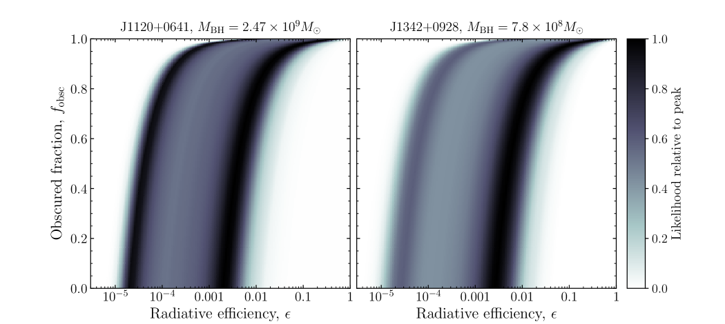
Figure 6: Slice through the 3D likelihood of $\epsilon$, $f_{\rm obsc}$, and $\Delta M_{\rm BH}$ for J1120+0641 (left) and J1342+0928 (right) at $\Delta M_{\rm BH}$ equal to their respective measured black hole masses.

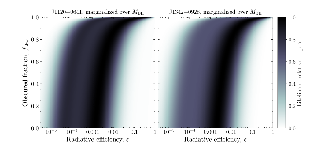
Figure 7: Similar to Figure 6, but now showing the joint likelihood of $\epsilon$ and $f_{\rm obsc}$ for J1120+0641 (left) and J1342+0928 (right) after marginalizing the 3D PDF from equation (B3) over a $\sigma=0.4$ dex lognormal systematic uncertainty in $M_{\rm BH}$.

We marginalize over $\Delta M_{\rm BH}$ with a lognormal prior centered on the measured black hole mass with a 1$\sigma$ width of 0.4 dex (Shen, 2013), resulting in the joint likelihood for $f_{\rm obsc}$ and $\epsilon$ shown in Figure 7. We then marginalize over $f_{\rm obsc}$ with a uniform prior from 0 to 100%. This prior on $f_{\rm obsc}$ reflects the fact that $\sim 50\%$ of quasars with similar luminosity at lower redshift are obscured (Polletta et al., 2008; Merloni et al., 2014) and that the evolution to $z>7$ is unknown. To subsequently derive the posterior PDF shown in Figure 3, we assume a log-uniform prior on $\epsilon$ from $10^{-7}$ to 1.

References

- Bañados et al. (2015) Bañados, E., Venemans, B. P., Morganson, E., et al. 2015, ApJ, 804, 118
- Bañados et al. (2018) Bañados, E., Venemans, B. P., Mazzucchelli, C., et al. 2018, Nature, 553, 473
- Bolton et al. (2011) Bolton, J. S., Haehnelt, M. G., Warren, S. J., et al. 2011, MNRAS, 416, L70
- Bromm & Loeb (2003) Bromm, V., & Loeb, A. 2003, ApJ, 596, 34
- Cen & Haiman (2000) Cen, R., & Haiman, Z. 2000, ApJ, 542, L75
- Comastri et al. (2015) Comastri, A., Gilli, R., Marconi, A., Risaliti, G., & Salvati, M. 2015, A&A, 574, L10
- Davies (2019) Davies, F. B. 2019, arXiv e-prints, arXiv:1904.10459
- Davies et al. (2016) Davies, F. B., Furlanetto, S. R., & McQuinn, M. 2016, MNRAS, 457, 3006
- Davies et al. (2019) Davies, F. B., Hennawi, J. F., & Eilers, A.-C. 2019, arXiv e-prints, arXiv:1903.12346
- Davies et al. (2018a) Davies, F. B., Hennawi, J. F., Bañados, E., et al. 2018a, ApJ, 864, 143
- Davies et al. (2018b) —. 2018b, ApJ, 864, 142
- Dayal & Ferrara (2018) Dayal, P., & Ferrara, A. 2018, Phys. Rep., 780, 1
- Eilers et al. (2017) Eilers, A.-C., Davies, F. B., Hennawi, J. F., et al. 2017, ApJ, 840, 24
- Eilers et al. (2018) Eilers, A.-C., Hennawi, J. F., & Davies, F. B. 2018, ApJ, 867, 30
- Ferrarese & Merritt (2000) Ferrarese, L., & Merritt, D. 2000, ApJ, 539, L9
- Gebhardt et al. (2000) Gebhardt, K., Bender, R., Bower, G., et al. 2000, ApJ, 539, L13
- Greig et al. (2017) Greig, B., Mesinger, A., Haiman, Z., & Simcoe, R. A. 2017, MNRAS, 466, 4239
- Heger et al. (2003) Heger, A., Fryer, C. L., Woosley, S. E., Langer, N., & Hartmann, D. H. 2003, ApJ, 591, 288
- Hopkins et al. (2005) Hopkins, P. F., Hernquist, L., Martini, P., et al. 2005, ApJ, 625, L71
- Khrykin et al. (2019) Khrykin, I. S., Hennawi, J. F., & Worseck, G. 2019, MNRAS, arXiv:1810.03391
- Koratkar & Blaes (1999) Koratkar, A., & Blaes, O. 1999, PASP, 111, 1
- Loeb & Furlanetto (2013) Loeb, A., & Furlanetto, S. R. 2013, The First Galaxies in the Universe
- Lukić et al. (2015) Lukić, Z., Stark, C. W., Nugent, P., et al. 2015, MNRAS, 446, 3697
- Lusso et al. (2015) Lusso, E., Worseck, G., Hennawi, J. F., et al. 2015, MNRAS, 449, 4204
- Madau et al. (2014) Madau, P., Haardt, F., & Dotti, M. 2014, ApJ, 784, L38
- Mazzucchelli et al. (2017) Mazzucchelli, C., Bañados, E., Venemans, B. P., et al. 2017, ApJ, 849, 91
- Merloni et al. (2014) Merloni, A., Bongiorno, A., Brusa, M., et al. 2014, MNRAS, 437, 3550
- Mesinger et al. (2011) Mesinger, A., Furlanetto, S., & Cen, R. 2011, MNRAS, 411, 955
- Miralda-Escudé (1998) Miralda-Escudé, J. 1998, ApJ, 501, 15
- Mortlock et al. (2011) Mortlock, D. J., Warren, S. J., Venemans, B. P., et al. 2011, Nature, 474, 616
- Nanni et al. (2017) Nanni, R., Vignali, C., Gilli, R., Moretti, A., & Brandt, W. N. 2017, A&A, 603, A128
- Omukai et al. (2008) Omukai, K., Schneider, R., & Haiman, Z. 2008, ApJ, 686, 801
- Polletta et al. (2008) Polletta, M., Weedman, D., Hönig, S., et al. 2008, ApJ, 675, 960
- Prochaska (2017) Prochaska, J. X. 2017, Astronomy and Computing, 19, 27
- Rees (1984) Rees, M. J. 1984, ARA&A, 22, 471
- Runnoe et al. (2012) Runnoe, J. C., Brotherton, M. S., & Shang, Z. 2012, MNRAS, 422, 478
- Sa̧dowski et al. (2014) Sa̧dowski, A., Narayan, R., McKinney, J. C., & Tchekhovskoy, A. 2014, MNRAS, 439, 503
- Schmidt (1963) Schmidt, M. 1963, Nature, 197, 1040
- Schmidt et al. (2018) Schmidt, T. M., Hennawi, J. F., Lee, K.-G., et al. 2018, arXiv e-prints, arXiv:1810.05156
- Shankar et al. (2009) Shankar, F., Weinberg, D. H., & Miralda-Escudé, J. 2009, ApJ, 690, 20
- Shen (2013) Shen, Y. 2013, Bulletin of the Astronomical Society of India, 41, 61
- Shen et al. (2018) Shen, Y., Wu, J., Jiang, L., et al. 2018, ArXiv e-prints, arXiv:1809.05584
- Soltan (1982) Soltan, A. 1982, MNRAS, 200, 115
- Tegmark et al. (1997) Tegmark, M., Silk, J., Rees, M. J., et al. 1997, ApJ, 474, 1
- Thorne (1974) Thorne, K. S. 1974, ApJ, 191, 507
- Trebitsch et al. (2019) Trebitsch, M., Volonteri, M., & Dubois, Y. 2019, MNRAS, 487, 819
- Ueda et al. (2014) Ueda, Y., Akiyama, M., Hasinger, G., Miyaji, T., & Watson, M. G. 2014, ApJ, 786, 104
- Venemans et al. (2016) Venemans, B. P., Walter, F., Zschaechner, L., et al. 2016, ApJ, 816, 37
- Venemans et al. (2017) Venemans, B. P., Walter, F., Decarli, R., et al. 2017, ApJ, 837, 146
- Vito et al. (2018) Vito, F., Brandt, W. N., Yang, G., et al. 2018, MNRAS, 473, 2378
- Volonteri & Rees (2005) Volonteri, M., & Rees, M. J. 2005, ApJ, 633, 624
- Wang et al. (2018) Wang, F., Yang, J., Fan, X., et al. 2018, ArXiv e-prints, arXiv:1810.11925
- Yang et al. (2018) Yang, J., Wang, F., Fan, X., et al. 2018, arXiv e-prints, arXiv:1811.11915
- Yu & Tremaine (2002) Yu, Q., & Tremaine, S. 2002, MNRAS, 335, 965