Fixed-time Control under Spatiotemporal and Input Constraints: A Quadratic Program Based Approach

Abstract

In this paper, we present a control synthesis framework for a general class of nonlinear, control-affine systems under spatiotemporal and input constraints. First, we study the problem of fixed-time convergence in the presence of input constraints. The relation between the domain of attraction for fixed-time stability with respect to input constraints and the required time of convergence is established. It is shown that increasing the control authority or the required time of convergence can expand the domain of attraction for fixed-time stability. Then, we consider the problem of finding a control input that confines the closed-loop system trajectories in a safe set and steers them to a goal set within a fixed time. To this end, we present a Quadratic Program (QP) formulation to compute the corresponding control input. We use slack variables to guarantee feasibility of the proposed QP under input constraints. Furthermore, when strict complementary slackness holds, we show that the solution of the QP is a continuous function of the system states, and establish uniqueness of closed-loop solutions to guarantee forward invariance using Nagumo’s theorem. We present two case studies, an example of adaptive cruise control problem and an instance of a two-robot motion planning problem, to corroborate our proposed methods.

, ,

1 Introduction

Driving the state of a dynamical system to a given desired point or a desired set in the presence of constraints is a problem of major practical importance. Constraints requiring the system trajectories to evolve in some safe set at all times while visiting some goal set(s) are common in safety-critical applications. Constraints pertaining to convergence to a goal set within a fixed time often appear in time-critical applications, e.g., when a task must be completed within a given time interval. Spatiotemporal specifications impose spatial (state) as well as temporal (time) constraints on the system trajectories. Figure 1 shows a scenario of a motivating problem requiring a quadrotor to remain in a domain (acting as a safe set), which consists of the region bounded by the green boundary excluding the regions marked in red. Furthermore, the blue regions denote the goal sets, which the quadrotor is required to visit in a given time sequence.

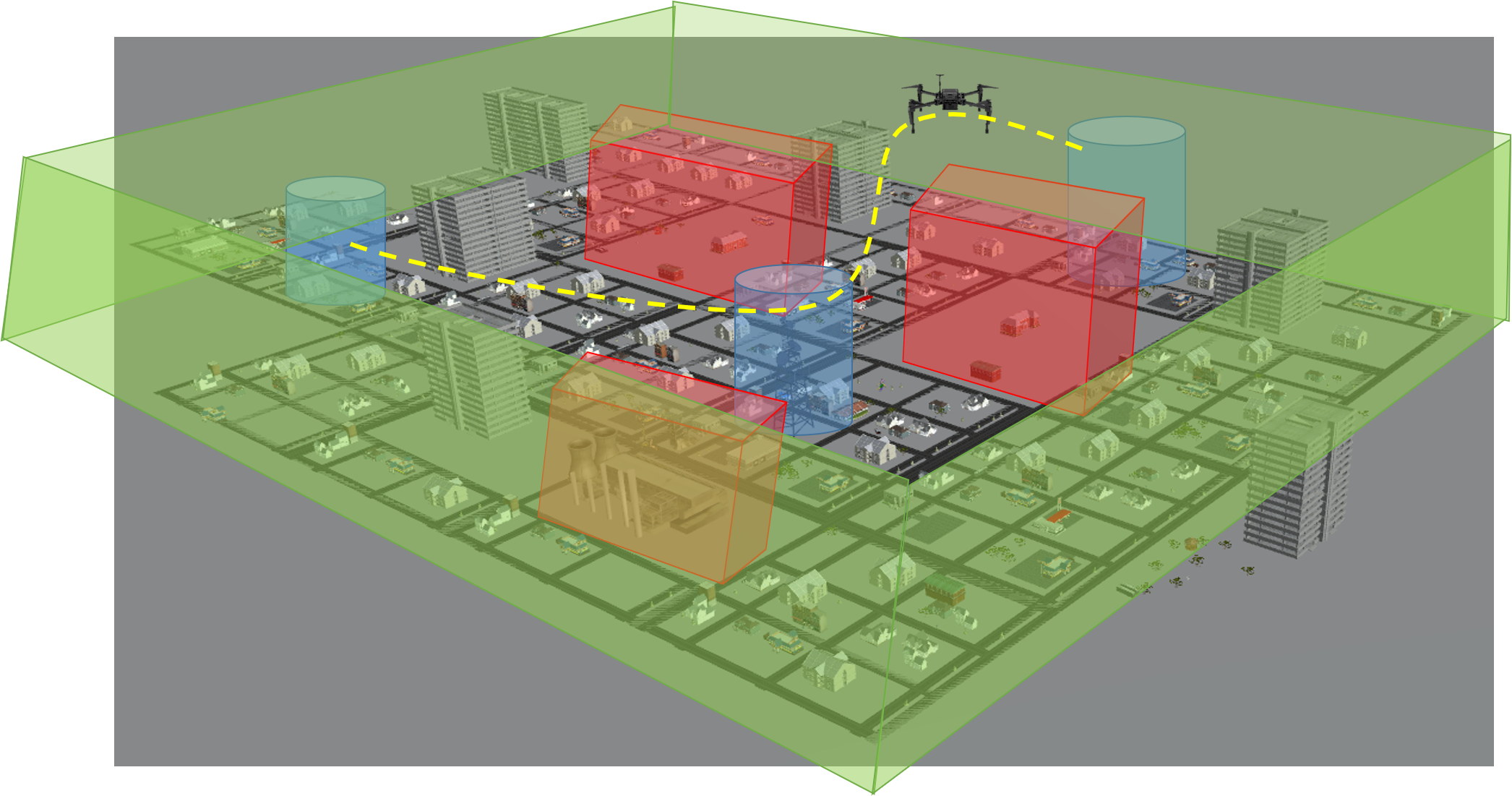
Figure 1: Motivating example scenario for a motion planning problem governed by spatiotemporal constraints.

Safety in dynamical systems is typically realized as establishing that a desired set of safe states, or safe set, is forward invariant under the system dynamics. The control objective reduces to designing a control law such that the closed-loop system trajectories remain always in the safe set. The approach in [28] utilizes Lyapunov-like barrier functions to guarantee that the system output always remains inside a given set. More recently, in [3], conditions using Zeroing Control Barrier Functions (ZCBF) are presented to ensure forward invariance of a desired set. Various approaches have been developed to achieve convergence of system trajectories to desired sets or points while satisfying control input constraints. Methods such as Model Predictive Control (MPC) [25, 13] as well as Control Lyapunov Functions (CLF) [27, 14] have been studied extensively in the literature. Quadratic Program (QP)-based approaches have gained popularity for control synthesis, see for instance [14, 27, 3, 22, 26]. These methods are suitable for real-time implementation as QPs can be solved efficiently [26, 11, 12]. The authors in [19] use an exponential barrier function in the QP formulation to guarantee safety of the closed-loop trajectories. In [31], safety barrier certificates are presented to ensure scalable collision-free behavior in multi-robot systems.

Concurrent forward invariance of a safe set and convergence to a goal set can be achieved via a combination of CLFs and Control Barrier Functions (CBFs), see e.g., [3, 24]. However, the concurrent satisfaction of the corresponding conditions and the underlying control synthesis problem become more challenging in the presence of input constraints, such as actuator saturation, since the latter may affect the region of safety and fixed-time convergence of the system trajectories. Most of the aforementioned contributions address control design that achieves safety along with convergence to a desired goal set (or point), but without explicitly considering control input constraints. Such constraints are considered in [3], where performance and safety objectives are represented using CLFs and CBFs, respectively, along with control input constraints in a QP.

Furthermore, most of the aforementioned work, with exception of [27, 14], deals with asymptotic or exponential convergence of the system trajectories to the desired goal point or goal sets. In contrast, Finite-Time Stability (FTS) is a concept that guarantees convergence in finite time. The authors in [5] introduce necessary and sufficient conditions in terms of a Lyapunov function for the equilibrium of a continuous-time, autonomous system to exhibit FTS. Fixed-Time Stability (FxTS) [21] is a stronger notion than FTS, where the time of convergence does not depend upon the initial conditions. For specifications involving temporal constraints and time-critical systems, the theory of finite- or fixed-time stability can be leveraged in the control design to guarantee that such specifications are met. It has also been shown that a faster rate of convergence generally implies that the closed-loop system has better disturbance rejection properties [5], which further motivates the study of finite- and fixed-time stable systems. The authors of [27] formulate a QP for finite-time convergence to a desired set, however without considering input constraints. This limitation is removed in [14], where the authors consider a QP formulation incorporating input, safety and convergence constraints. The authors in [16] use CBFs in a QP formulation to encode Signal-Temporal Logic (STL) specifications that impose reaching to a goal set within a finite time.

In this paper, we study the problem of reaching a given goal set $S_{G}$ within a fixed time $T_{ud}$, while remaining in a given safe set $S_{S}$ at all times, for a general class of nonlinear control-affine systems with input constraints. In the preliminary conference version [9], a QP formulation is proposed to compute the control input for fixed-time convergence under input and safety constraints, yet without any guarantees on the feasibility of the proposed method. Per its definition, FxTS of an equilibrium point from arbitrary initial conditions presumes unbounded control authority. To address the problem of FxTS in the presence of input constraints, new Lyapunov conditions from [10] are utilized. When used in a QP, the new Lyapunov conditions introduce a slack term, which results in feasibility guarantees in the presence of input constraints. The contributions of the paper as follows:

• First, FxTS conditions are utilized in a QP, and using Karush-Kuhn-Tucker (KKT) conditions, the closed-form expression for the optimal value of the slack term is computed for the case when the control input is saturated. Then, the relation between the Domain of Attraction (DoA) for FxTS, the input bounds, and the fixed time of convergence is established for a 1-D control-affine system.

• Then, a novel QP formulation that utilizes Fixed-Time (FxT) CLFs and CBFs is proposed to synthesize controllers for nonlinear, control-affine systems, so that forward invariance of a safe set and FxT convergence of the system trajectories to a goal set is guaranteed. We use slack terms both in the safety and the FxT convergence constraints to ensure that the QP is always feasible even in the presence of control input constraints.

• Conditions for continuity of the control input as the optimal solution of the QP are studied under milder conditions as compared to prior work, and it is shown that the closed-loop solutions are uniquely determined so that forward invariance of the safe set can be established.

Compared to the earlier literature, the contributions of this paper are summarized as follows. The QP-based approaches in the prior literature, e.g., [14, 27, 19, 30, 31, 2, 3, 16, 9], do not provide feasibility guarantees for the underlying QP in the presence of input constraints. However, without feasibility of the QP, it is not guaranteed that a control input can be always synthesized, and without consideration of input bounds, the resulting input might not be realizable on a real-world platform. In comparison to these prior studies, we consider control input constraints in addition to the safety and convergence requirements, and guarantee the feasibility of the proposed QP. The proposed approach further advances the results in [27, 15, 14] in terms of the achieved time of convergence. Furthermore, we generalize the results of [3, 18, 11], where the regularity properties of the solution of the QP is discussed in the absence of input constraints; we show continuity of the solution of the proposed QP under the presence of input constraints, and under milder regularity assumptions on the CLF, CBF, and the system dynamics, as compared to the aforementioned work.

Organization: The rest of the paper is organized as follows. The main problem formulation is discussed in Section 2. Mathematical preliminaries of safety and fixed-time stability are reviewed in Section 3. New results on fixed-time stability under input constraints are presented in Section 4. The main results on QP-based control synthesis are presented in Section 5. Section 6 presents two numerical case studies and Section 7 concludes the paper with some directions for future work.

2 Problem Formulation

In the rest of the paper, ${\mathbb{R}}$ denotes the set of real numbers and $\mathbb{R}_{+}$ denotes the set of non-negative real numbers. We use $\|\cdot\|_{p}$ to denote the $p-$norm, and $\|\cdot\|$ to denote the Euclidean norm. We write $\partial S$ for the boundary of a closed set $S\in\mathbb{R}^{n}$, $\textnormal{int}(S)\coloneqq S\setminus\partial S$ for its interior, and $|x|_{S}=\inf_{y\in S}\|x-y\|$ for the distance of a point $x\in\mathbb{R}^{n}\setminus S$ from the set $S$. We use $\mathcal{C}^{k}$ to denote the set of $k$ times continuously differentiable functions. The Lie derivative of a $\mathcal{C}^{1}$ function $V:\mathbb{R}^{n}\rightarrow\mathbb{R}$ along a vector field $f:\mathbb{R}^{n}\rightarrow\mathbb{R}^{n}$ at a point $x\in\mathbb{R}^{n}$ is denoted as $L_{f}V(x)\coloneqq\frac{\partial V}{\partial x}f(x)$. For two vectors $x,y\in\mathbb{R}^{n}$, we use $x\leq y$ to represent element-wise inequalities $x_{i}\leq y_{i},i=1,2,\ldots,n$. A continuous function $\alpha:\mathbb{R}_{+}\rightarrow\mathbb{R}_{+}$ is a class-$\mathcal{K}$ function if it is strictly increasing and $\alpha(0)=0$. It belongs to $\mathcal{K}_{\infty}$ if in addition, $\lim_{r\to\infty}\alpha(r)=\infty$. A function $\kappa:\mathbb{R}_{+}\times\mathbb{R}_{+}\rightarrow\mathbb{R}_{+}$ is a class-$\mathcal{KL}$ function if 1) for all $t\geq 0$, the map $\kappa(r,t)$ belongs to class-$\mathcal{K}$ and 2) for all $r\geq 0$, the map $\kappa(r,t)$ is decreasing in $t$ with $\kappa(r,t)\to 0$ as $t\to\infty$. A function $V:\mathbb{R}^{n}\rightarrow\mathbb{R}$ is said to be positive definite with respect to a compact set $S\subset\mathbb{R}^{n}$ if $V(x)>0$ for $x\notin S$ and $V(x)=0$ for $x\in\partial S$. We drop the arguments $t,x$ whenever clear from the context.

Next, we present the problem formulation. Consider the nonlinear, control-affine system

$$\dot{x}(t)=f(x(t))+g(x(t))u(x(t)),\quad x(0)=x_{0},$$ (1)

where $x\in\mathbb{R}^{n}$ is the state vector, $f:\mathbb{R}^{n}\rightarrow\mathbb{R}^{n}$ and $g:\mathbb{R}^{n}\rightarrow\mathbb{R}^{n\times m}$ are system vector fields, continuous in their arguments, and $u\in\mathcal{U}\subset\mathbb{R}^{m}$ is the control input vector where $\mathcal{U}$ is the input constraint set. In addition, consider a safe set $S_{S}\coloneqq\{x\;|\;h_{S}(x)\leq 0\}$ to be rendered forward invariant under the closed-loop dynamics of (1), and a goal set $S_{G}\coloneqq\{x\;|\;h_{G}(x)\leq 0\}$ to be reached by the closed-loop trajectories of (1) in a user-defined fixed time $T_{ud}>0$, where $h_{S},h_{G}:\mathbb{R}^{n}\rightarrow\mathbb{R}$ satisfy the following assumption.

Assumption 1.

The functions $h_{S}(x),h_{G}(x)\in\mathcal{C}^{1}$, $S_{G}\bigcap S_{S}\neq\emptyset$, the set $S_{G}$ is compact, and the sets $S_{S}$ and $S_{G}$ have non-empty interiors. Furthermore, the function $h_{G}$ is proper with respect to set $S_{G}$, i.e., there exists a class-$\mathcal{K}_{\infty}$ function $\alpha_{G}$ such that $h_{G}(x)\geq\alpha_{G}(|x|_{S_{G}})$, for all $x\notin S_{G}$.

Note that the boundary and the interior of set $S_{S}$ (and similarly, of the set $S_{G}$) are given as $\partial S_{S}\coloneqq\{x\;|\;h_{S}(x)=0\}$ and $\textnormal{int}(S_{S})\coloneqq\{x\;|\;h_{S}(x)<0\}$, respectively. Next, we define the notion of fixed-time domain of attraction for a compact set $S\subset\mathbb{R}^{n}$:

Definition 1 (FxT-DoA).

For a compact set $S\subset\mathbb{R}^{n}$, the set $D\subset\mathbb{R}^{n}$, satisfying $S\subset D$, is a Fixed-Time Domain of Attraction (FxT-DoA) with time $T>0$ for the closed-loop system (1) under $u$, if

• for all $x(0)\in D$, $x(t)\in D$ for all $t\in[0,T]$, and

• there exists $T_{0}\in[0,T]$ such that $\lim_{t\to T_{0}}x(t)\in S$.

In words, a FxT-DoA for a set $S\subset\mathbb{R}^{n}$ is a set $D\supset S$ such that it is forward-invariant and starting from any point within the set $D$, the system trajectories reach the set $S$ within a fixed-time $T$. We can now state the main problem considered in this paper.

Problem 1.

Design a control input $u(x)\in\mathcal{U}\coloneqq\{v\in\mathbb{R}^{m}\;|\;A_{u}v\leq b_{u}\}$ and compute $D\subset\mathbb{R}^{n}$, so that for all $x_{0}\in D\subseteq S_{S}$, the closed-loop trajectories $x(t)$ of (1) satisfy $x(t)\in S_{S}$ for all $t\geq 0$, and $x(T_{ud})\in S_{G}$, where $T_{ud}>0$ is a user-defined fixed time and $D$ is a FxT-DoA for the set $S_{G}$.

Input constraints of the form $\mathcal{U}=\{v\in\mathbb{R}^{m}\;|\;A_{u}v\leq b_{u}\}$ are very commonly considered in the literature, see e.g., [26, 3]. In Section 5, we present a quadratic program that computes a control input $u$ that solves Problem 1. Before that, we present mathematical preliminaries in the next section.

3 Preliminaries

3.1 Forward invariance of safe set

Problem 1 requires that the closed-loop system trajectories of (1) stay in the set $S_{S}$ at all times, i.e., the set $S_{S}$ is forward-invariant. Forward invariance of a set is defined as follows:

Definition 2.

A set $S\subset\mathbb{R}^{n}$ is forward invariant for the closed-loop system (1) under the effect of a control input $u(x(t))$ if $x_{0}\in S$ implies that $x(t)\in S$ for all $t\geq 0$.

The following result, known as Nagumo’s theorem, is adapted from [6] for forward invariance of the set $S_{S}$ for the control system (1):

Lemma 1 (Nagumo’s theorem).

Let $u(x)\in\mathcal{U}$ be a continuous control input such that the resulting closed-loop trajectories of (1) are uniquely determined in forward time. Then, the set $S_{S}$ is forward invariant for the closed-loop system (1) if and only if the following holds:

$$L_{f}h_{S}(x)+L_{g}h_{S}(x)u(x)\leq 0\quad\forall x\in\partial S_{S}.$$ (2)

The interested reader is referred to [6, Section 3.1] for a detailed discussion on forward invariance of sets. We make the following assumption to guarantee that the safe set $S_{S}$ can be rendered forward invariant for (1).

Assumption 2.

For all $x\in\partial S_{S}$, there exists a control input $u(x)\in\mathcal{U}$ such that the following condition holds:

$$L_{f}h_{S}(x)+L_{g}h_{S}(x)u(x)\leq 0.$$ (3)

Similar assumptions have been used in literature, either explicitly (e.g., [24]) or implicitly (e.g., [3]). In this work, we use the following notion of ZCBFs to ensure forward invariance of the safe set $S_{S}$. The ZCBF is defined by the authors in [3] as follows:

Definition 3 (ZCBF).

For the dynamical system (1), a continuously differentiable function $h:\mathbb{R}^{n}\rightarrow\mathbb{R}$ is called a ZCBF for the set $S_{S}$ if $h(x)<0$ for $x\in\textnormal{int}(S_{S})$, $h(x)=0$ for $x\in\partial S_{S}$, and there exists $\alpha\in\mathcal{K}$, such that

$$\inf_{u\in\mathcal{U}}\{L_{f}h(x)+L_{g}h(x)u\}\leq\alpha(-h(x))\quad\forall x\in S_{S}.$$ (4)

It is easy to see that if $h$ is a ZCBF, then it also satisfies Assumption 2. One special case of (4) is

$$\inf_{u\in\mathcal{U}}\{L_{f}h(x)+L_{g}h(x)u\}\leq-\rho h(x),$$ (5)

with $\rho>0$, as discussed in [3, Remark 6]. We will use this special form (5) in our main results to guarantee forward invariance of the safe set $S_{S}$.

3.2 Overview of fixed-time stability

Next, we review the notion of fixed-time stability. The authors in [21] define the origin to be an FxTS equilibrium of (1) if it is Lyapunov stable and $\lim_{t\to T}x(t)=0$ where the time of convergence $T=T(x(0))$ is uniformly bounded for all $x(0)$, i.e., $\sup\limits_{x(0)\in\mathbb{R}^{n}}T(x(0))<\infty$. The following sufficient conditions for FxTS of the origin are adapted from [20].

Lemma 2.

Let $V:\mathbb{R}^{n}\rightarrow\mathbb{R}$ be a continuously differentiable, positive definite, radially unbounded function, satisfying

$$\inf_{u\in\mathcal{U}}\{L_{f}V(x)+L_{g}V(x)u\}\leq-\alpha_{1}V(x)^{\gamma_{1}}-\alpha_{2}V(x)^{\gamma_{2}},$$ (6)

for all $x\in\mathbb{R}^{n}\setminus\{0\}$, with $\alpha_{1},\alpha_{2}>0$, $\gamma_{1}=1+\frac{1}{\mu}$ and $\gamma_{2}=1-\frac{1}{\mu}$ for some $\mu>1$. Then, the origin of (1) is FxTS with $T$ that satisfies $T\leq\frac{\mu\pi}{2\sqrt{\alpha_{1}\alpha_{2}}}$.

Inspired by [17], we define a class of CLF for the system (1), which is used to encode the convergence of the system trajectories to a compact set $S\subset\mathbb{R}^{n}$ within a user-defined, fixed time $T_{ud}$:

Definition 4 (FxT CLF-$S$).

A continuously differentiable function $V:\mathbb{R}^{n}\rightarrow\mathbb{R}$ is called FxT CLF-$S$ for (1) with parameters $\alpha_{1},\alpha_{2}>0,\gamma_{1}=1+\frac{1}{\mu},\gamma_{2}=1-\frac{1}{\mu}$ with $\mu>1$, if $V$ is proper w.r.t. set $S$ and the following holds:

$$\inf_{u\in\mathcal{U}}\{L_{f}V(x)+L_{g}V(x)u\}\leq-\alpha_{1}V(x)^{\gamma_{1}}-\alpha_{2}V(x)^{\gamma_{2}},$$ (7)

for all $x\in\mathbb{R}^{n}\setminus S$, where the time of convergence $T$ satisfies $T\leq\frac{\mu\pi}{2\sqrt{\alpha_{1}\alpha_{2}}}\leq T_{ud}$.

4 Fixed-time stability under input constraints

4.1 Motivating example

In this section, we review new FxTS conditions from our recent work in [10]. These conditions are motivated by, and used in, the control synthesis under fixed-time convergence and input constraints, and are essential in guaranteeing the feasibility of the proposed QP. Consider, for the sake of illustration, a 1-dimensional control-affine system

$$\dot{x}=f(x)+g(x)u,$$ (8)

where $f,g:\mathbb{R}\rightarrow\mathbb{R}$ are continuous functions. Suppose that the control objective is to drive the closed-loop trajectories of (8) to a set $S_{V}\coloneqq\{x\;|\;V(x)\leq 0\}$ within a user-defined time $T_{ud}$, where $V:\mathbb{R}\rightarrow\mathbb{R}$ is continuously differentiable, and proper with respect to the set $S_{V}$. Additionally, consider the input constraints $u_{m}\leq u\leq u_{M}$ where $u_{m}<u_{M}$. To this end, following the work in [3, 19] and using the FxTS conditions from Lemma 2, a QP can be formulated as follows:

$$\min_{u}\;\;\quad\frac{1}{2}u^{2}$$ (9a)

$$\textrm{s.t.}\quad\begin{bmatrix}1\\ -1\end{bmatrix}u\leq \begin{bmatrix}u_{M}\\ -u_{m}\end{bmatrix},$$ (9b)

$$L_{f}V(x)+L_{g}V(x)u\leq -\alpha_{1}V(x)^{\gamma_{1}}-\alpha_{2}V(x)^{\gamma_{2}},$$ (9c)

for $x\notin S_{V}$, where $c>0$, and $\alpha_{1},\alpha_{2},\gamma_{1},\gamma_{2}$ are chosen as $\alpha_{1}=\alpha_{2}=\frac{\mu\pi}{2T_{ud}}$, $\gamma_{1}=1+\frac{1}{\mu}$ and $\gamma_{2}=1-\frac{1}{\mu}$ with $\mu>1$. Existence of the solution of (9) implies existence of a control input under which the closed-loop trajectories of (8) reach the set $S_{V}$ within a fixed time $T$ that satisfies $T\leq\frac{\mu\pi}{2\sqrt{\alpha_{1}\alpha_{2}}}$; therefore, by setting $\alpha_{1}=\alpha_{2}=\frac{\mu\pi}{2T_{ud}}$, it follows that $T\leq T_{ud}$, i.e., the convergence will be achieved within the user-define time. The issue with the QP in (9) is that it might not be feasible for all $x\in\mathbb{R}^{n}\setminus S_{V}$ due to the presence of the input constraints. To address the issue of infeasibility of a QP under multiple constraints, the authors in [3] introduce a slack variable in the CLF constraint. Inspired from this, the new FxTS conditions are presented next.

4.2 New FxTS Lyapunov conditions

Lemma 3 ([10]).

Let $V:\mathbb{R}^{n}\rightarrow\mathbb{R}$ be a continuously differentiable, positive definite, radially unbounded function, satisfying

$$\begin{split}\inf_{u\in\mathcal{U}}\{L_{f}V(x)+L_{g}V(x)u\}\leq&\ \delta_{1}V(x)-\alpha_{1}V(x)^{\gamma_{1}}\\ &-\alpha_{2}V(x)^{\gamma_{2}},\end{split}$$ (10)

for all $x\in\mathbb{R}^{n}\setminus\{0\}$, with $\alpha_{1},\alpha_{2}>0$, $\delta_{1}\in\mathbb{R}$, $\gamma_{1}=1+\frac{1}{\mu}$, $\gamma_{2}=1-\frac{1}{\mu}$ for some $\mu>1$. Then, $D\subset\mathbb{R}^{n}$ is a FxT-DoA of the origin of (1) with time $T>0$, where

$$D =\begin{cases}\;\mathbb{R}^{n};&r<1,\\ \left\{x\;|\;V(x)\leq k^{\mu}\left(\frac{\delta_{1}-\sqrt{\delta_{1}^{2}-4\alpha_{1}\alpha_{2}}}{2\alpha_{1}}\right)^{\mu}\right\};&r\geq 1,\end{cases},$$ (11)

$$T \leq\begin{cases}\frac{\mu\pi}{2\sqrt{\alpha_{1}\alpha_{2}}};&r\leq 0,\\ \frac{\mu}{\alpha_{1}k_{1}}\left(\frac{\pi}{2}-\tan^{-1}k_{2}\right);&0\leq r<1,\\ \frac{\mu k}{(1-k)\sqrt{\alpha_{1}\alpha_{2}}};&r\geq 1,\end{cases},$$ (12)

where $r=\frac{\delta_{1}}{2\sqrt{\alpha_{1}\alpha_{2}}}$, $0<k<1$, $k_{1}=\sqrt{\frac{4\alpha_{1}\alpha_{2}-\delta_{1}^{2}}{4\alpha_{1}^{2}}}$ and $k_{2}=-\frac{\delta_{1}}{\sqrt{4\alpha_{1}\alpha_{2}-\delta_{1}^{2}}}$.

In comparison to Lemma 2, Lemma 3 allows an additional (possibly, positive) term $\delta_{1}V$ in the upper bound of the time derivative of the Lyapunov function. The main idea is to use (10) in place of the constraint (9c), with the parameters $\alpha_{1},\alpha_{2},\mu$ chosen such that $\frac{\mu\pi}{2\sqrt{\alpha_{1}\alpha_{2}}}=T_{ud}$, and with $\delta_{1}$ being a free, slack variable so that feasibility of the QP can be guaranteed. Then, the value of $\delta_{1}$ would dictate the FxT-DoA $D$. To see how the condition (10) can be used to guarantee FxTS in the presence of control input constraints, a new QP can be formulated as follows:

$$\min_{u,\delta_{1}}\;\frac{1}{2}u^{2} +\frac{1}{2}\delta_{1}^{2}+c\delta_{1}$$ (13a)

$$\textrm{s.t.}\quad\quad\begin{bmatrix}1\\ -1\end{bmatrix}u\leq \begin{bmatrix}u_{M}\\ -u_{m}\end{bmatrix},$$ (13b)

$$L_{f}V(x)+L_{g}V(x)u\leq \;\delta_{1}V(x)-\alpha_{1}V(x)^{\gamma_{1}}-\alpha_{2}V(x)^{\gamma_{2}},$$ (13c)

for $x\notin S_{V}$, where $c>0$, and $\alpha_{1},\alpha_{2},\gamma_{1},\gamma_{2}$ are chosen similarly as in (9). Note that when $\delta_{1}$ takes negative values, then out of (12) the bound on the time of convergence satisfies $T\leq\frac{\mu\pi}{2\sqrt{\alpha_{1}\alpha_{2}}}=T_{ud}$, and therefore, convergence within the user-defined time $T_{ud}$ can be achieved. Thus, the linear term $c\delta_{1}$ is introduced in the cost function with $c>0$ in order to penalize non-positive values of $\delta_{1}$. Here, the term $\delta_{1}V(x)$ in (13c) can be thought of as a slack term, allowing for satisfaction of the constraint (13c) in the presence of input constraints (13b) as shown below.

Lemma 4.

For each $x\notin S_{V}$, there exist $u(x)\in\mathbb{R},\delta_{1}(x)\in\mathbb{R}$ satisfying (13b)-(13c), i.e., the QP (13) is feasible for all $x\notin S_{V}$.

Choose any $\bar{u}(x)\in[u_{m},u_{M}]$ so that $\bar{u}(x)$ satisfies the input constraints. For $x\notin S_{V}$ we have that $V(x)>0$ and therefore,

$$\bar{\delta}_{1}(x)\coloneqq\frac{L_{f}V(x)+L_{g}V(x)\bar{u}(x)+\alpha_{1}V(x)^{\gamma_{1}}+\alpha_{2}V(x)^{\gamma_{2}}}{V(x)},$$

is well-defined for all $x\notin S_{V}$. Note that with $u=\bar{u}(x),\delta_{1}=\bar{\delta}_{1}(x)$, (13c) is satisfied with equality. Thus, the pair $(\bar{u}(x),\bar{\delta}_{1}(x))$ satisfies (13b)-(13c) for all $x\notin S_{V}$, and thus, the QP (13) is feasible for all $x\notin S_{V}$.

Note that in prior work, e.g. [3, 19], the slack term is used as

$$L_{f}V(x)+L_{g}V(x)u\leq\delta-cV(x),$$

for some $c>0$. While this condition helps guarantee feasibility of the underlying QP, it does not guarantee that the function $V(x)$ reaches its zero sub-level set when $\delta>0$. Per Lemma 3, it holds that the system trajectories reach the zero sub-level set of the function $V(x)$ even when $\delta>0$. This is a unique contribution of the new FxTS condition in Lemma 3.

4.3 Relation of FxT-DoA with input constraints and time of convergence

As mentioned above, the slack term $\delta_{1}$ is used to guarantee feasibility of the underlying QP. Now, the relation of this slack term with FxT-DoA, input constraints and the fixed time of convergence is explored. Let us hypothesize that the slack term corresponding to $\delta_{1}$ in the QP (13) characterizes the trade-off between the FxT-DoA and the time of convergence for given control input bounds, and between the FxT-DoA and the input bounds for a given fixed time of convergence. In the particular case when $\alpha_{1}=\alpha_{2}=\alpha$ for some $\alpha>0$, let us examine how the FxT-DoA $D$ in (11) is affected by the ratio $r^{\star}(x)=\frac{\delta^{\star}(x)}{2\alpha}$, where $(u^{\star}(x),\delta^{\star}(x))$ is the optimal solution of the QP (13). Define $r_{M}=\sup_{x\in S}r^{\star}(x)$. For $r_{M}<1$, it holds that $D=\mathbb{R}^{n}$, which is the largest possible FxT-DoA. For $r_{M}\geq 1$, it holds that

$$D =\left\{x\;|\;V(x)\leq\inf_{z\in S}k^{\mu}\left(\frac{\delta_{1}^{\star}(z)-\sqrt{(\delta_{1}^{\star}(z))^{2}-4\alpha_{1}\alpha_{2}}}{2\alpha_{1}}\right)^{\mu}\right\}$$

$$=\left\{x\;|\;V(x)\leq\inf_{z\in S}k^{\mu}\left(r^{\star}(z)-\sqrt{(r^{\star}(z))^{2}-1}\right)^{\mu}\right\}.$$

It can be readily verified that $\left(r-\sqrt{r^{2}-1}\right)$ is a monotonically decreasing function for $r\geq 1$ and therefore, it holds that

$$D =\left\{x\;|\;V(x)\leq k^{\mu}\left(r_{M}-\sqrt{r_{M}^{2}-1}\right)^{\mu}\right\}.$$ (14)

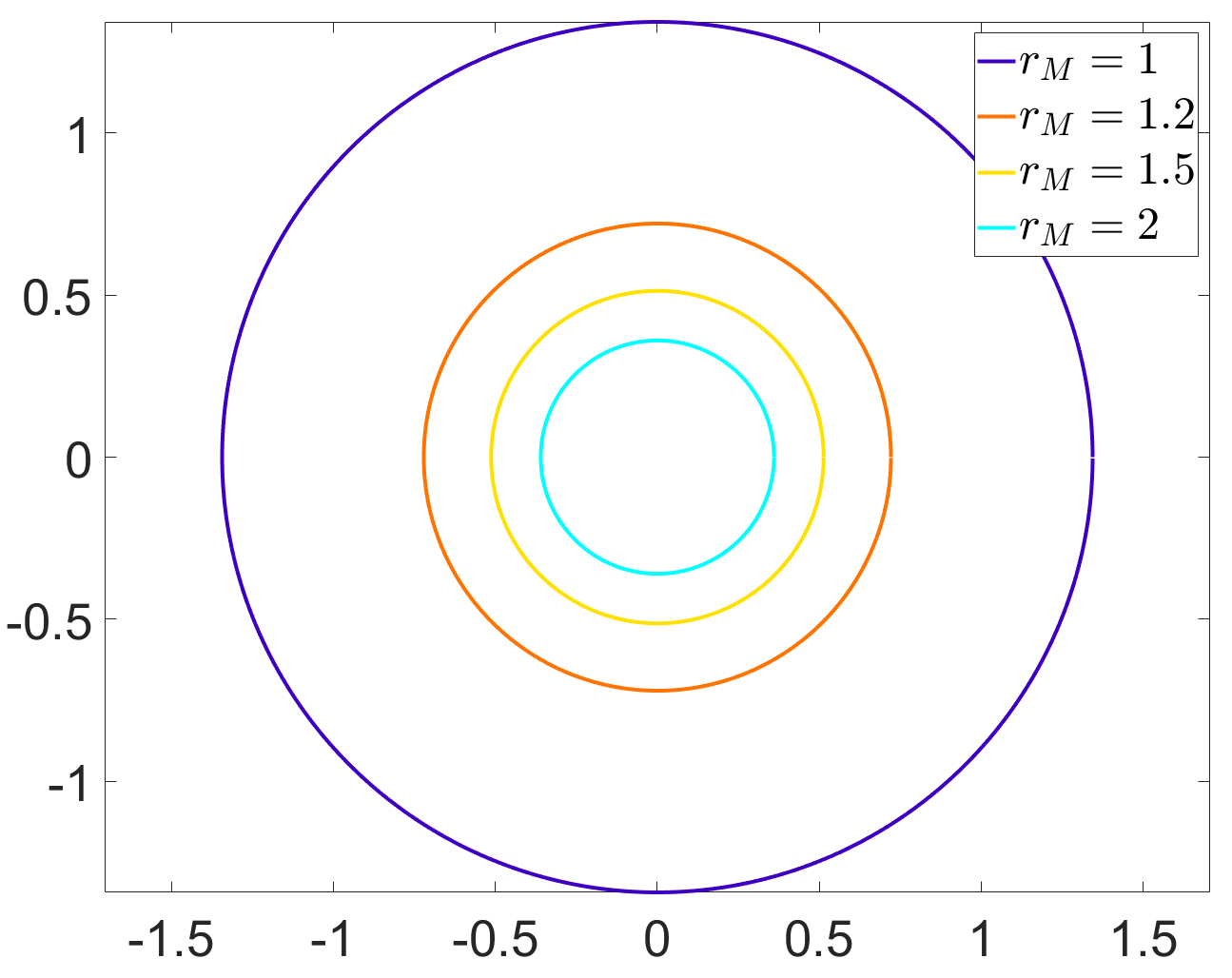
Figure 2: FxT-DoA $D$ for $k=0.95$ and $\mu=2$.

Figure 2 plots the FxT-DoA $D$ for $V(x)=\frac{1}{2}\|x\|^{2}$. It can be concluded, based on (14), that the domain $D$ shrinks as $r_{M}$ increases, which is also demonstrated in Figure 2. Thus, the larger the FxT-DoA $D$ is, the smaller the value of $r_{M}$ is. Now, the following Lemma establishes the closed-form expression for the slack variable $\delta_{1}^{\star}(x)$ in the particular case when the control input is saturated with $u^{\star}(x)=u_{M}$ for the QP (13).

Lemma 5.

Consider the QP (13) and let $a(x)\coloneqq L_{f}V(x)+L_{g}V(x)u_{M}+cV(x)+\alpha_{1}V(x)^{\gamma_{1}}+\alpha_{2}V(x)^{\gamma_{2}}$. Then, for $x\in S_{M}$ where

$$S_{M}\coloneqq\{x\;|\;a(x)L_{g}V(x)+u_{M}V(x)^{2}<0,a(x)>0\},$$

the optimal value of $u$ is given as $u^{\star}(x)=u_{M}$, and the optimal value of $\delta_{1}$ is given as

$$\begin{split}\delta_{1}^{\star}(x)=&\frac{L_{f}V(x)+L_{g}V(x)u_{M}}{V(x)}+\alpha_{1}V(x)^{\gamma_{1}-1}\\ &+\alpha_{2}V(x)^{\gamma_{2}-1}.\end{split}$$ (15)

The proof is provided in Appendix A. Recall that the QP (13) is defined for $x\notin S_{V}$. Note that for $x\in S_{M}\setminus S_{V}$, $L_{g}V(x)<0$ (per definition of the set $S_{M}$) and $V(x)>0$ (since $V$ is proper w.r.t. the set $S_{V}$). Define $r^{\star}(x)\coloneqq\frac{\delta_{1}(x)^{\star}}{2\sqrt{\alpha_{1}\alpha_{2}}}$ so that

$$\begin{split}r^{\star}(x)=&\left(\frac{L_{f}V(x)+L_{g}V(x)u_{M}}{V(x)}\right)\frac{T_{ud}}{\mu\pi}+\frac{1}{2}V(x)^{\gamma_{1}-1}\\ &+\frac{1}{2}V(x)^{\gamma_{2}-1}.\end{split}$$ (16)

For a given $x\in S_{M}\setminus S_{V}$, the expression for the optimal value of $r$ in (16) is a function of the fixed time of convergence $T_{ud}$, and of the upper-bound on the control input $u_{M}$. Since the region of interest is the one from where the closed-loop trajectories converge to the set $S_{V}$, consider (16) for the case when $x\in S\coloneqq S_{M}\cap\{x\;|\;L_{f}V(x)+L_{g}V(x)u_{M}<0\}$. For the restricted domain $S$, it is clear that $r^{\star}$ decreases as the control authority increases (i.e., as $u_{M}$ increases), or the time of convergence requirement relaxes (i.e., as $T_{ud}$ increases). Based on this and (14), it is concluded that for a given input bound, relaxing $T_{ud}$ results in a larger FxT-DoA $D$, and conversely, for a given $T_{ud}$, increasing the input bounds results into a larger FxT-DoA. Thus, the hypothesis that the slack variable $\delta_{1}$ characterizes the trade-off between the FxT-DoA, time of convergence, and the input bounds is verified.

5 Main results

5.1 QP formulation

In this section, a control synthesis approach is presented to address Problem 1. First, a QP is designed with guaranteed feasibility, then it is shown that the solution of the QP is a continuous function of $x$, and finally, some sufficient conditions are presented under which Problem 1 is solved by the optimal solution of the proposed QP. In what follows, unless specified otherwise, all the results are presented under Assumptions 1-2. Define $z=\begin{bmatrix}v^{T}&\delta_{1}&\delta_{2}\end{bmatrix}^{T}\in\mathbb{R}^{m+2}$, and consider the following QP:

$$\min_{z\in\mathbb{R}^{m+2}}\;\frac{1}{2}z^{T}Hz +F^{T}z$$ (17a)

$$\textrm{s.t.}\quad\;A_{u}v\leq \;b_{u},$$ (17b)

$$L_{f}h_{G}(x)+L_{g}h_{G}(x)v\leq \;\delta_{1}h_{G}(x)-\alpha_{1}\max\{0,h_{G}(x)\}^{\gamma_{1}}$$

$$-\alpha_{2}\max\{0,h_{G}(x)\}^{\gamma_{2}}$$ (17c)

$$L_{f}h_{S}(x)+L_{g}h_{S}(x)v\leq -\delta_{2}h_{S}(x),$$ (17d)

where $H=\textrm{diag}\{w_{u_{1}},\ldots,w_{u_{m}},w_{1},w_{2}\}$ is a diagonal matrix consisting of positive weights $w_{u_{i}},w_{i}>0$, $F=\begin{bmatrix}\mathbf{0}_{m}^{T}&q_{1}&0\end{bmatrix}$ with $q_{1}>0$ and $\mathbf{0}_{m}\in\mathbb{R}^{m}$ a column vector consisting of zeros. The parameters $\alpha_{1},\alpha_{2},\gamma_{1},\gamma_{2}$ are fixed, and are chosen as $\alpha_{1}=\alpha_{2}=\frac{\mu\pi}{2T_{ud}}$, $\gamma_{1}=1+\frac{1}{\mu}$ and $\gamma_{2}=1-\frac{1}{\mu}$ with $\mu>1$. The choice of these parameters does not affect the feasibility of the QP, as discussed below. In principle, any value of $\mu$ can be chosen as long as it is greater than 1. The linear term $F^{T}z=q_{1}\delta_{1}$ in the objective function of (17) penalizes the positive values of $\delta_{1}$ (see Theorem 2 for details on why $\delta_{1}$ being non-positive could be useful). Constraint (17b) guarantees that the control input satisfies the control input constraints. Per Lemma 3, the constraint (17c) guarantees convergence and the constraint (17d) ensures safety.

The slack terms corresponding to $\delta_{1},\delta_{2}$ allow the upper bounds of the time derivatives of $h_{S}(x)$ and $h_{G}(x)$, respectively, to have a positive term for $x$ such that $h_{S}(x)<0$ and $h_{G}(x)>0$. This ensures the feasibility of the QP (17) for all $x$, as demonstrated below.

Lemma 6.

Under Assumptions 1-2, for each $x\in S_{S}\setminus S_{G}$, there exist $v(x)\in\mathbb{R}^{m},\delta_{1}(x)\in\mathbb{R},\delta_{2}(x)\in\mathbb{R}$ satisfying (17b)-(17d), i.e., the QP (17) is feasible for all $x\in S_{S}\setminus S_{G}$.

Since $x\notin S_{G}$, it holds that $h_{G}(x)>0$. Consider the following two cases separately: $h_{S}(x)=0$ and $h_{S}(x)<0$.

First, let $h_{S}(x)<0$, i.e., $x\in\textrm{int}(S_{S})$. Since $\mathcal{U}$ is non-empty, there exists $v=\bar{v}$ in $\mathcal{U}$ such that $\eqref{C1 cont const}$ is satisfied. Choose $\bar{\delta}_{2}\coloneqq\frac{L_{f}h_{S}(x)+L_{g}h_{S}(x)\bar{v}}{-h_{S}(x)}$, so that (17d) is satisfied with equality. Also, for $x\in\textrm{int}(S_{S})\setminus S_{G}$, it holds that $h_{G}(x)>0$. Define $\bar{\delta}_{1}\coloneqq\frac{L_{f}h_{G}(x)+L_{g}h_{G}(x)\bar{v}+\alpha_{1}h_{G}(x)^{\gamma_{1}}+\alpha_{2}h_{G}(x)^{\gamma_{2}}}{h_{G}(x)}$, so that (17c) holds with equality. Thus, for the case when $h_{S}(x)<0$, there exists $(\bar{v},\bar{\delta}_{1},\bar{\delta}_{2})$ such that (17b)-(17d) holds.

Next, let $h_{S}(x)=0$, i.e., $x\in\partial S_{S}$. Per Assumption 2, it holds that that there exists $v=\tilde{v}\in\mathcal{U}$ such that (17d) holds. Since $h_{S}(x)=0$, any value of $\delta_{2}$ is feasible, and hence, one can choose $\delta_{2}=0$. Hence, the choice of $(v,\delta_{1},\delta_{2})=(\tilde{v},\bar{\delta}_{1},0)$ satisfies (17b)-(17d). Thus, the QP (17) is always feasible.

One of the main novelties of the QP (17) is the way the slack variables are introduced in the FxT-CLF and the ZCBF constraints. Not only these slack variables guarantee that the QP remains feasible under input constraints, they also do not jeopardise forward-invariance of the set $S_{S}$ or convergence to the goal set $S_{G}$. In particular, keeping in mind the discussion given after the proof of Lemma 5, the traditional ZCBF condition in the prior work, e.g. [3, 11, 12, 14, 27], uses a particular value of $\delta_{2}$ for the safety constraint. In the proposed formulation, this parameter is kept as a free variable, so that both safety and feasibility of the QP can be guaranteed simultaneously.

5.2 Continuity of the solution of the QP

Guaranteeing forward invariance of the safe set $S_{S}$ is based on Lemma 1, which in turn requires the uniqueness of the system solutions. Traditionally, Lipschitz continuity of the right-hand side of (1) is utilized in order to guarantee existence and uniqueness of the solutions of (1), see e.g., [3, 32, 16]. When the right-hand side of (1) is only continuous, existence and uniqueness of the solutions can be established using the results in [1, Section 3.15-3.18] (see Lemma 7). To this end, first, it is shown that the control input $u(x)$ as a solution of the QP (17) is continuous in its arguments. Define $A:\mathbb{R}^{n}\rightarrow\mathbb{R}^{(2m+2)\times(m+2)}$ and $b:\mathbb{R}^{n}\rightarrow\mathbb{R}^{(2m+2)}$ as

$$A(x) \coloneqq\begin{bmatrix}A_{u}&{{\mathbf{0}_{2m}}}&{{\mathbf{0}_{2m}}}\\ L_{g}h_{G}(x)&-h_{G}(x)&0\\ L_{g}h_{S}(x)&0&h_{S}(x)\end{bmatrix},\;b(x)\coloneqq\begin{bmatrix}b_{u}\\ b_{2}(x)\\ -L_{f}h_{S}(x)\end{bmatrix}$$

where $b_{2}(x)\coloneqq-L_{f}h_{G}(x)-\alpha_{1}\max\{0,h_{G}(x)\}^{\gamma_{1}}-\alpha_{2}\max\{0,h_{G}(x)\}^{\gamma_{2}}$ and $\mathbf{0}_{2m}\in\mathbb{R}^{2m}$ is a column vector consisting of zeros. Also, define the functions $G_{i}(x,z)\coloneqq A_{i}(x)z-b_{i}(x)$ where $A_{i}\in\mathbb{R}^{1\times(m+2)}$ is the $i$-th row of the matrix $A$, and $b_{i}\in\mathbb{R}$ the $i$-th element of $b$, so that the constraints (17b)-(17d) can be written as $G_{i}(x,z)\leq 0$ for $i\in 1,2,\ldots,2m+2$. Let $z^{\star}$ and $\lambda^{\star}\in\mathbb{R}_{+}^{2m+2}$ denote the optimal solution of (17), and the corresponding optimal Lagrange multiplier, respectively. The following assumption is made to prove the main results of this section.

Assumption 3.

The strict complementary slackness holds for (17) for all $x\in\textnormal{int}(S_{S})\setminus S_{G}$, i.e., for each $i\in\{1,2,\dots,2m+2\}$, it holds that either $\lambda_{i}^{\star}>0$ or $G_{i}(x,z^{\star})<0$ for all $x\in\textnormal{int}(S_{S})\setminus S_{G}$.

Complementary slackness, i.e., $\lambda_{i}^{\star}G_{i}(x,z^{\star})=0$, for all $i=1,\ldots,2m+2$, is a both necessary and sufficient condition for optimality of the solution for QPs [7, Chapter 5]. Note that this condition permits that for some $i$, both $\lambda_{i}^{\star}=0$ and $G_{i}(x,z^{\star})=0$. Strict complementary slackness rules out this possibility, and requires that for each $i$, either $\lambda_{i}^{\star}$ or $G_{i}(x,z^{\star})$ is non-zero.

Theorem 1.

Under Assumptions 1 and 3, the solution $z^{\star}:\mathbb{R}^{n}\rightarrow\mathbb{R}^{m+2}$ of (17) is continuous on $\textnormal{int}(S_{S})\setminus S_{G}$.

The proof is provided in Appendix B.

A note on comparison to earlier work: Note that the above result guarantees that the control input defined as $u(x)=v^{\star}(x)$ is continuous on $\textnormal{int}(S_{S})\setminus S_{G}$. Under Assumption 3, the authors in [8] show that the solution is continuously differentiable if the objective function and the constraints functions are twice continuously differentiable. The authors in [3] assume that the functions $f,g$ and the Lie derivatives $L_{f}h_{S},L_{f}h_{G},L_{g}h_{S},L_{g}h_{G}$ are locally Lipschitz continuous to show Lipschitz continuity of the solution of QP in the absence of control input constraints. Under similar assumptions, the authors in [11] show that the solution of QP is guaranteed to be Lipschitz continuous (in the absence of input constraints) if the CBF constraints are inactive, i.e., the constraints are satisfied with strict inequality at the optimal solution $z^{\star}$, which is same as Assumption 3. Note that in the presented formulation, the only requirement is that the functions $f,g$ are continuous, and $h_{S},h_{G}$ continuously differentiable in $x$, which is a relaxation of the prior assumptions. Note also that the authors of [11] extend their results in [12] by utilizing the theory of non-smooth analysis, and strong forward invariance of sets even if the control input is not continuous. Under similar assumptions, the results in [29] utilize the concept of Clarke tangent cones to guarantee strong forward invariance when the control input is only Lebesgue measurable.

Next, it is shown that closed-loop trajectories of (1) under $u=v^{\star}$ exist and are unique.

Lemma 7.

Let Assumptions 1-3 hold. If the solution of (17), given as $z^{\star}=[v^{\star}(\cdot)^{T}\;\delta_{1}^{\star}(\cdot)\;\delta_{2}^{\star}(\cdot)]^{T}$, satisfies $\mathfrak{d}_{1}\coloneqq\sup\limits_{\textnormal{int}(S_{S})\setminus S_{G}}\delta_{1}^{\star}(x)<\infty$, then there exists a neighborhood $D$ of the set $S_{G}$ such that the closed-loop trajectory under $u(x)=v^{\star}(x)$ exists and is unique for all $t\geq 0$ and for all $x(0)\in D$. Furthermore, if $\mathfrak{d}_{1}\leq 0$, then the result holds with $D=S_{S}$.

The proof is based on [1, Theorem 3.18.1]. Using [1, Theorem 3.15.1] and choosing a Lyapunov candidate $\mathfrak{v}=\frac{1}{2}|y|^{2}$, it can be shown that $y\equiv 0$ is the unique solution of $\dot{y}=0$ for $y(0)=0$. Theorem 1 guarantees that the solution of the QP (17) is continuous, which implies continuity of the closed-loop system dynamics (1) when $u(x)\coloneqq v^{\star}(x)$. Note that $h_{G}(x)=0$ for $x\in\partial S_{G}$ and $h_{G}(x)>0$ for $x\notin S_{G}$, i.e., the function $h_{G}$ is positive definite with respect to the set $S_{G}$. Define $\phi(y)\coloneqq\mathfrak{d}_{1}y-\alpha_{1}\operatorname{sign}(y)|y|^{\gamma_{1}}-\alpha_{2}\operatorname{sign}(y)|y|^{\gamma_{2}}$. Per Lemma 3, it holds that there exists a neighborhood $D_{y}\subset\mathbb{R}$ of the origin such that for all $y\in D_{y}$, $\phi(y)\leq 0$. Thus, there exists a function $g$ defined as $g(t,V)=0$ that satisfies condition (i) of [1, Theorem 3.18.1], the closed-loop dynamics of (1) satisfies the condition (ii), and there exists a function $V$ defined as $V(x)=h_{G}(x)$ that satisfies the condition (iii). Thus, using [1, Theorem 3.18.1], there exists $\tau>0$ such that the solution of the closed-loop system (1) exists and is unique for all $x(0)\in D=\{x\;|\;V(x)\in D_{y}\}$ and all $t\in[0,\tau)$. Since the closed-loop solution $x(t)$ is bounded in the compact set $D$, the solution is complete (see [4, Ch2., Theorem 1]), and thus, $\tau=\infty$.

Finally, in the case when $\mathfrak{d}_{1}\leq 0$, it holds that the $D_{y}=\mathbb{R}$, and thus, the result holds with $D=S_{S}$.

5.3 Safety and fixed-time convergence

Finally, it is shown that under some conditions, the solution of (17) solves Problem 1.

Theorem 2.

Let Assumptions 1-3 hold. If the solution of (17), given as $z^{\star}=[v^{\star}(\cdot)^{T}\;\delta_{1}^{\star}(\cdot)\;\delta_{2}^{\star}(\cdot)]^{T}$, satisfies $\delta_{1}^{\star}(x)\leq 0,\ \ \forall x\in\textnormal{int}(S_{S})$, then, $u(\cdot)=v^{\star}(\cdot)$ solves Problem 1 for all $x(0)\in\textnormal{int}(S_{S})$, i.e., $D=\textnormal{int}(S_{S})$.

First, the convergence of the closed-loop trajectories $x(t)$ to the set $S_{G}$ within the user-defined time $T_{ud}$ is shown. Since $\delta_{1}^{\star}(x)\leq 0$, per Lemma 3, it holds that the closed-loop trajectories of (1) with $u(x)\coloneqq v^{\star}(x)$ reach the set $S_{G}$ within fixed time $T\leq\frac{\mu\pi}{2(\alpha_{1}\alpha_{2})^{\frac{1}{2}}}=T_{ud}$, i.e., within the user-defined time $T_{ud}$ for all $x(0)\in\textnormal{int}(S_{S})$.

Next, it is shown that the closed-loop trajectories of (1) satisfy $x(t)\in\textnormal{int}(S_{S})$ for all $t\leq T_{ud}$ under $u(x)\coloneqq v^{\star}(x)$. From Lemma 7, it holds that the closed-loop solution of (1) exists and is unique under $u=v^{\star}$ for all $0\leq t\leq T_{ud}$ and for all $x(0)\in\textnormal{int}(S_{S})$. Using the similar arguments as in [3, Theorem 1], it can be shown that the set $\textnormal{int}(S_{S})$ is forward-invariant. Therefore, the control input $u(x)\coloneqq v^{\star}(x)$ solves Problem 1 for all $x(0)\in\textnormal{int}(S_{S})$.

Remark 1.

As pointed out in [3], the conflict between safety and the convergence constraint require a non-zero slack term for satisfaction of (17c)-(17d) together. With this observation and keeping in mind the discussion in Section 4, one can readily conclude that if the control-input bounds or the user-defined time $T_{ud}$ is sufficiently large, then it is possible to satisfy (17c) with $\delta_{1}\leq 0$.

Remark 2.

Utilizing the notion of FxT CLF from Definition 4, it can be shown that the function $h_{G}$ being FxT CLF-$S_{G}$ is a sufficient condition for the solution of the QP (17) to generate a control input that solves Problem 1. In particular, if $h_{G}$ is an FxT CLF-$S_{G}$ for (1) with parameters $\alpha_{1},\alpha_{2},\gamma_{1},\gamma_{2}$ as defined in (17), then the QP (17) with $\delta_{1}=0$ is feasible for all $x\in\textnormal{int}(S_{S})\setminus S_{G}$, i.e., the solution $(v^{\star}(x),\delta_{2}^{\star}(x))$ of the QP (17) after fixing $\delta_{1}=0$ exists for all $x\in\textnormal{int}(S_{S})\setminus S_{G}$.

Next, some cases are listed when the solution of QP (17) might not solve Problem 1 with the specified time constraint and from all initial conditions, but it still renders the closed-loop trajectories safe, and convergent to the set $S_{G}$ within some fixed time.

Theorem 3.

Under Assumptions 1-3, the following hold:

• If the solution of (17) satisfies

  $$\mathfrak{d}_{1}\coloneqq\sup_{x\in S_{S}\setminus S_{G}}\delta_{1}^{\star}(x) <2\sqrt{\alpha_{1}\alpha_{2}}=\frac{\mu\pi}{T_{ud}},$$ (18)

  then, for all $x(0)\in\textnormal{int}(S_{S})$, the closed-loop trajectories $x(t)$ of (1) under $u(x)\coloneqq v^{\star}(x)$ reach the set $S_{G}$ in a fixed time

  $$T_{1}\leq\frac{\mu}{\alpha_{1}\mathrm{k}_{1}}\left(\frac{\pi}{2}-\tan^{-1}\mathrm{k}_{2}\right),$$

  where $\mathrm{k}_{1}\coloneqq\sqrt{\frac{4\alpha_{1}\alpha_{2}-\mathfrak{d}_{1}}{4\alpha_{1}^{2}}}$ and $\mathrm{k}_{2}\coloneqq-\frac{\mathfrak{d}_{1}}{\sqrt{4\alpha_{1}\alpha_{2}-\mathfrak{d}_{1}}}$, while satisfying $x(t)\in S_{S}$ for all $t\geq 0$, i.e., $D=\textnormal{int}(S_{S})$.

• If (18) does not hold, then there exists $D\subset\textnormal{int}(S_{S})$ such that for all $x(0)\in D$, the closed-loop trajectories satisfy $x(t)\in\textnormal{int}(S_{S})$ for all $t\geq 0$ and reach the goal set $S_{G}$ within a fixed time

  $$T_{2}\leq\frac{\mu k}{(1-k)\sqrt{\alpha_{1}\alpha_{2}}},$$

  where $0<k<1$, where $D$ is the largest sub-level set of the function $h_{G}$ in the set $D_{G}\cap\textnormal{int}(S_{S})$, with $D_{G}=\{x\;|\;h_{G}(x)\leq k^{\mu}\left(\frac{\mathfrak{d}_{1}-\sqrt{\mathfrak{d}_{1}-4\alpha_{1}\alpha_{2}}}{2\alpha_{1}}\right)^{\mu}\}$.

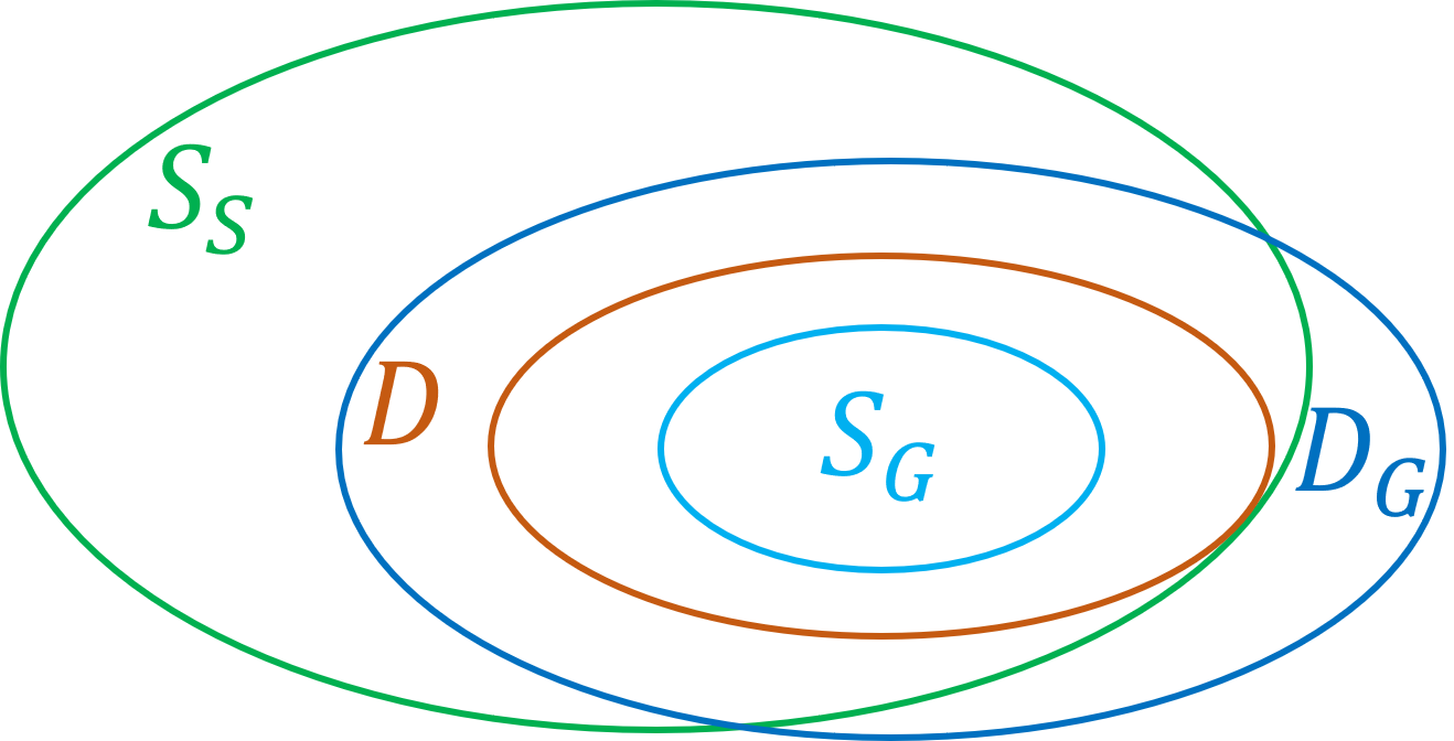
Figure 3: Illustration of the safe set $S_{S}$ (shown in green), the goal set $S_{G}$ (shown in light blue), FxT-DoA $D_{G}$ for the goal set (shown in dark blue) and the domain $D$ (shown in brown).

In both cases, following the proof of Theorem 2, it holds that the closed-loop trajectories satisfy $x(t)\in\textnormal{int}(S_{S})$ for all $0\leq t\leq T$ for any $T<\infty$. When (18) holds, using Lemma 3, it follows that the closed-loop trajectories $x(t)$ of (1) under $u(x)\coloneqq v^{\star}(x)$ reach the set $S_{G}$ within fixed time $T_{1}$ for all $x(0)\in\textnormal{int}(S_{S})$ satisfying $T_{1}\leq\frac{\mu}{\alpha_{1}\mathrm{k}_{1}}\left(\frac{\pi}{2}-\tan^{-1}\mathrm{k}_{2}\right)$, where $\mathrm{k}_{1}\coloneqq\sqrt{\frac{4\alpha_{1}\alpha_{2}-\mathfrak{d}_{1}}{4\alpha_{1}^{2}}}$ and $\mathrm{k}_{2}\coloneqq-\frac{\mathfrak{d}_{1}}{\sqrt{4\alpha_{1}\alpha_{2}-\mathfrak{d}_{1}}}$. Also, per (18), it holds that $\mathrm{k}_{1}>0$ and so, $T_{1}<\infty$.

For the case when (18) does not hold, using Lemma 3, it holds that the closed-loop trajectories of (1) under $u(x)\coloneqq v^{\star}(x)$ reach the set $S_{G}$ within time $T_{2}$ for all $x(0)\in D_{G}$ where $T_{2}\leq\frac{\mu k}{(1-k)\sqrt{\alpha_{1}\alpha_{2}}}$ and $D_{G}\coloneqq\left\{x\;|\;h_{G}(x)\leq k^{\mu}\left(\frac{\mathfrak{d}_{1}-\sqrt{\mathfrak{d}_{1}-4\alpha_{1}\alpha_{2}}}{2\alpha_{1}}\right)^{\mu}\right\}$, where $0<k<1$. Since it is also required that $x(0)\in\textnormal{int}(S_{S})$, define $D$ as the largest sub-level set of the function $h_{G}$ in the set $D_{G}\cap\textnormal{int}(S_{S})$, so that $D$ is forward invariant (see Figure 3). Therefore, for all $x(0)\in D$, the closed-loop trajectories of (1) reach the set $S_{G}$ within the fixed time $T_{2}$, while maintaining safety at all times.

In brief, the solution of the QP (17) always exists, is a continuous function of $x$, and renders the set $\textnormal{int}(S_{S})$ forward invariant, i.e., guarantees safety. Furthermore, the control input is guaranteed to yield fixed-time convergence of the closed-loop trajectories to the goal set $S_{G}$. In the case when $\delta_{1}\leq 0$, the convergence is guaranteed for all $x(0)\in\textnormal{int}(S_{S})$, and within the user-defined fixed time $T_{ud}$. If $\delta_{1}$ satisfies (18), then fixed-time convergence is guaranteed for all $x(0)\in\textnormal{int}(S_{S})$ (i.e., $D=\textnormal{int}(S_{S})$), but the time of convergence $T_{1}$ may exceed the time $T_{ud}$. Finally, if (18) does not hold, then fixed-time convergence is guaranteed for all $x(0)\in D\subset\textnormal{int}(S_{S})$, however, the time of convergence $T_{2}$ may exceed the time $T_{ud}$.

6 Numerical Case Studies

We present two case studies to illustrate the efficacy of the proposed method. We use Euler discretization to discretize the continuous-time dynamics, and the Matlab function quadprog to solve the QP at each discrete time step.

6.1 Adaptive Cruise Control Problem

In this example, we consider an adaptive cruise control (ACC) problem with a following and a lead vehicle, where the objective for the following vehicle is to achieve a desired speed, and maintain a safe distance from the lead vehicle. Considering that the two vehicles are modeled as point masses and travelling along a straight line, the system dynamics can be written as $\dot{x}=f(x)+gu$ with $f(x)=\begin{bmatrix}-F_{r}(x)/M&a_{L}&x_{2}-x_{1}\end{bmatrix}^{T},g=\begin{bmatrix}1/M&0&0\end{bmatrix}^{T}$, where $u\in[-u_{\max},u_{\max}]$ is the control input, $x=[x_{1},x_{2},x_{3}]^{T}=[v_{f},v_{l},D]^{T}\in{\mathbb{R}}^{3}$ is the system state with $v_{f}$ being the velocity of the following vehicle, $v_{l}$ being the velocity of the lead vehicle, and $D$ being the distance between the two vehicles (see [3] for more details). Here, $M$ is the mass of the following vehicle, $F_{r}(x)=f_{0}+f_{1}v_{f}+f_{2}v_{f}^{2}$ is the drag force, and $a_{L}\in(-a_{l}\mathbf{a}_{g},a_{l}\mathbf{a}_{g})$ is the acceleration of the lead vehicle, with $a_{l}$ being the fraction of the gravitational acceleration $\mathbf{a}_{g}$.

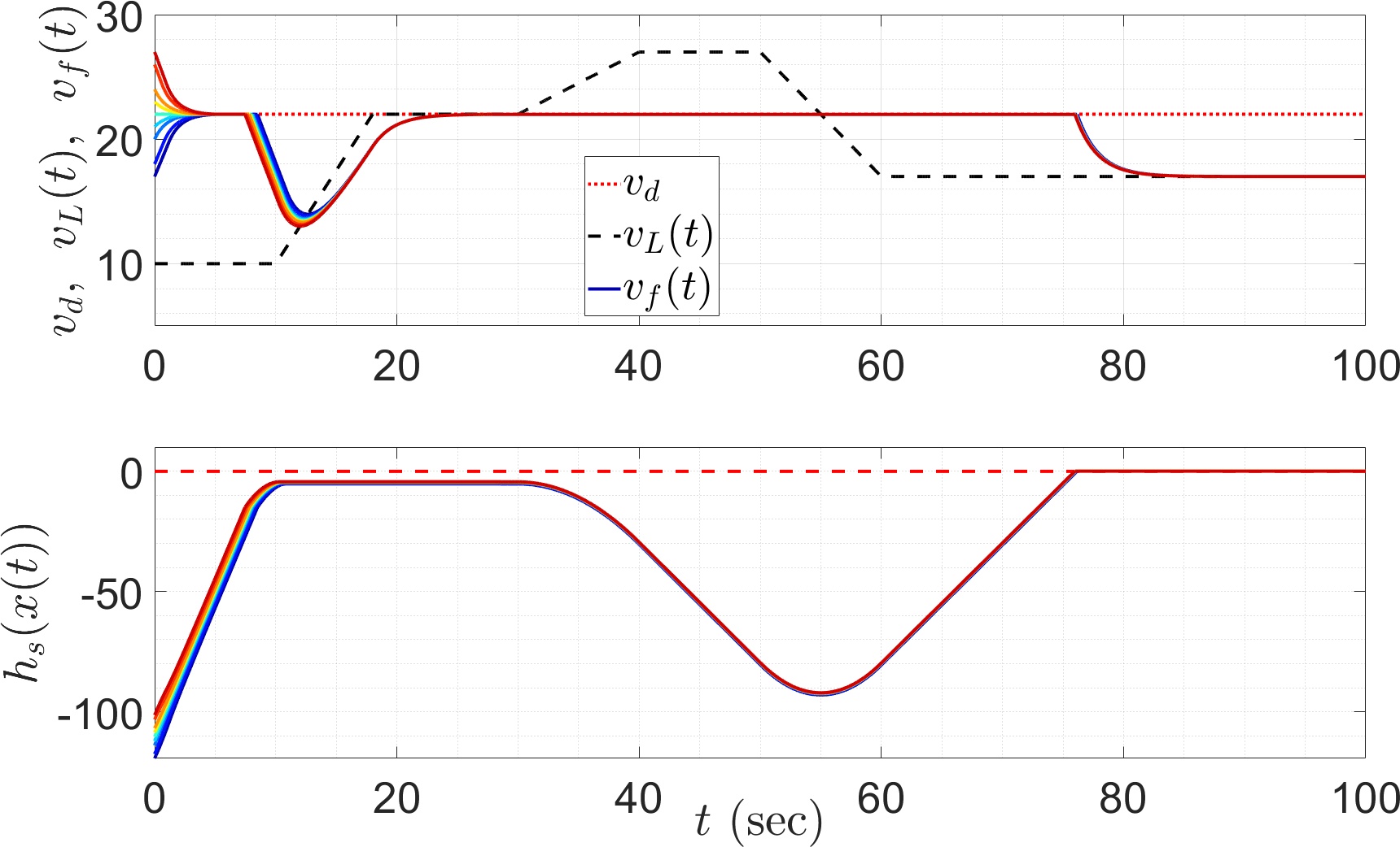
Figure 4: Tracking Performance and the safe set $h_{S}(x)$ for various initial follower velocities $v_{f}(0)\in[17,27]$ $\mathrm{m/s}$ with $T=10$ sec.

We define the goal and the safe sets, respectively, using the functions $h_{G}(x)=(v_{f}-v_{d})^{2},h_{S}(x)=\tau_{d}v_{f}-D,$ where $v_{d}$ is a desired fixed velocity and $\tau_{d}$ is the desired time headway. We set the maximum available control effort to $u_{\max}=0.25M\mathbf{a}_{g}$ with $\mathbf{a}_{g}=9.81$ $\mathrm{m/s^{2}}$ and $M=1650$ $\mathrm{Kg}$, the desired velocity to $v_{d}=22$ $\mathrm{m/s}$, the initial velocity of the lead vehicle to $v_{l}(0)=10$ $\mathrm{m/s}$, initial distance to $D(0)=150$ $\mathrm{m}$, $f_{0}=0.1$ $\mathrm{N}$, $f_{1}=5$ $\mathrm{Ns/m}$, $f_{2}=0.25$ $\mathrm{Ns^{2}/m^{2}}$, and $a_{l}=0.3$. We implement the QP in (17) with $T_{ud}=10$ sec, and $\mu=5$ resulting in $\gamma_{1}=1.2$, $\gamma_{2}=0.8$.

Figures 4 and 5 illustrate the tracking performance of the resulting controller, where the solid lines represent the velocity of the following vehicle for different initial velocity of the following vehicle $v_{f}(0)\in[17,27]$ $\mathrm{m/s}$. The desired speed is achieved when the trajectories are away from the boundaries of the safe set, while closer to the boundaries of the safe set the speed of the following vehicle is reduced to maintain safety.

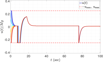
Figure 5: Control input for the closed-loop trajectories for various $v_{f}(0)$.

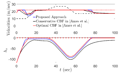
Figure 6: Tracking performance comparison of the proposed approach and the results in [3] (referenced as [Ames et al.]). The reference velocity is shown in black dotted line and the lead vehicle’s velocity in red dotted line.

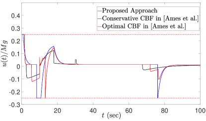
Figure 7: Control input for the proposed approach and the results in [3].

As stated before, there is no guarantee for the existence of the solution of the proposed QP in [3] when there is a control input constraint. For the specific problem of adaptive cruise control as in this example, the authors in [3] introduced two control barrier functions, namely optimal and conservative CBFs, based on the simplified system dynamics with no drag effect $F_{r}(x)$ to ensure feasibility of the solution. However, due to conservatism, the newly constructed safe sets $h_{F}^{o}(x)$ and $h_{F}^{c}(x)$ for the optimal and conservative CBFs are violated initially for large initial velocity of the following vehicle, while the actual safe set $h_{S}(x)=\tau_{d}v_{f}-D$ is not violated and the problem can be still feasible.

Figure 8: Energy for the proposed approach and the results in [3].

Figures 6 and 7 compare the tracking performance of the proposed approach and the results with optimal and conservative CBFs with $v_{f}(0)=18$ $\mathrm{m/s}$. Since we are solving the QP directly and without the aforementioned conservatism, one can see from Figure 6 that our proposed control approach tracks the desired goal speed of $22$ $\mathrm{m/s}$ for a longer duration before departure from this speed for maintaining safety.

Finally, Figure 8 compares the control effort between the the proposed approach and the results in [3], where the proposed approach is using more available control authority. This is due to the fact that the desired goal speed is tracked for a longer duration in the proposed approach, and hence more control action is used to keep the system trajectories in the safe set as the trade-off.

6.2 Motion planning with spatiotemporal specifications

In the second scenario, we present a two-agent motion planning example under spatiotemporal specifications, where the robot dynamics are modeled under constrained unicycle dynamics as

$$\dot{x}_{i} =u_{i}\cos(\theta_{i}),$$ (19a)

$$\dot{y}_{i} =u_{i}\sin(\theta_{i}),$$ (19b)

$$\dot{\theta}_{i} =\omega_{i},$$ (19c)

where $[x_{i}\;\ y_{i}]^{T}\in\mathbb{R}^{2}$ is the position vector of the agent $i$ for $i\in\{1,2\}$, $\theta_{i}\in\mathbb{R}$ its orientation and $[u_{i}\;\ \omega_{i}]^{T}\in\mathbb{R}^{2}$ the control input vector comprising of the linear speed $u_{i}\in[0,u_{M}]$ and angular velocity $|\omega_{i}|\leq\omega_{M}$. The closed-loop trajectories for the agents, starting from $[x_{1}(0)\;\ y_{1}(0)]^{T}\in C_{1}=\{z\in\mathbb{R}^{2}\;|\;\|z-[-1.5\;1.5]^{T}\|_{\infty}\leq 0.5\}$ and $[x_{2}(0)\;\ y_{2}(0)]^{T}\in C_{2}=\{z\in\mathbb{R}^{2}\;|\;\|z-[1.5\;1.5]^{T}\|_{\infty}\leq 0.5\}$, respectively, are required to reach to sets $C_{2}$ and $C_{1}$, while staying inside the blue rectangle $\{z\in\mathbb{R}^{2}\;|\;\|z\|_{\infty}\leq 2\}$, and outside the red-dotted circle $\{z\in\mathbb{R}^{2}\;|\;\|z\|_{2}\leq 1.5\}$, as shown in Figure 9. The agents are also required to maintain a minimum inter-agent distance $d_{m}>0$ at all times.

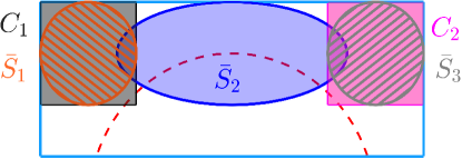
Figure 9: Problem setting and sets $\bar{S}_{1},\bar{S}_{2},\bar{S}_{3}$ for simulation example 2.

Note that the sets $C_{i}$ are not overlapping with each other, and the corresponding functions $h_{i}(x)$ are not continuously differentiable. Thus, to satisfy Assumption 2 and use the QP (17), we construct auxiliary sets $\bar{S}_{1}=\{[x\;\ y]\;|\;\frac{(x+1.5)^{2}}{0.5^{2}}+\frac{(y-1.5)^{2}}{0.5^{2}}\leq 1\}$ (orange circle), $\bar{S}_{2}=\{[x\;\ y]^{T}\;|\;\frac{x^{2}}{1.2^{2}}+\frac{(y-1.5)^{2}}{0.5^{2}}\leq 1\}$ (blue ellipse) and $\bar{S}_{3}=\{[x\;\ y]^{T}\;|\;\frac{(x-1.5)^{2}}{0.5^{2}}+\frac{(y-1.5)^{2}}{0.5^{2}}\leq 1\}$ (grey circle) as shown in Figure 9.

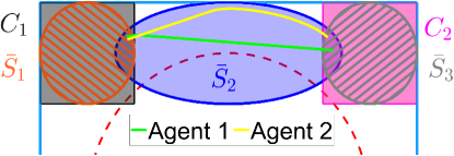
Figure 10: The resulting closed-loop paths of the agents.

We choose the barrier functions as

$$h_{ij}(x_{1},x_{2},y_{1},y_{2}) =d_{m}^{2}-\|[x_{1}-x_{2}\;\ y_{1}-y_{2}]^{T}\|^{2}$$ (20a)

$$h_{1}(x,y) =1.5^{2}-\|[x\;\ y]^{T}\|^{2},$$ (20b)

$$h_{2}(x,y) =[x\;\ y-1.5]P[x\;\ y-1.5]^{T}-1,$$ (20c)

$$h_{\theta}(\theta) =0.1^{2}-(\theta-\phi-\pi)^{2},$$ (20d)

where $P=\begin{bmatrix}1/1.5^{2}&0\\ 0&1/0.5^{2}\end{bmatrix}$ and $\phi\triangleq\angle([x\;\ y]^{T})$ is the angle of the position vector $[x\;\ y]^{T}$ from the $x-$axis. The functions $h_{1}$ and $h_{2}$, along with $h_{\theta}$, help keep the agent inside the set $\bar{S}_{2}$ and outside the red-dotted circle, respectively, in Figure 9. We choose the Lyapunov function as

$$V_{1} =(x-x_{g})^{2}+(y-y_{g})^{2}-0.5^{2},$$ (21a)

$$V_{\theta} =(\theta-\phi_{g})^{2}-0.1^{2},$$ (21b)

where $[x_{g}\;\ y_{g}]^{T}=[1.5\;\ 1.5]^{T}$ is the goal location and $\phi_{g}=\angle([x_{g}\;\ y_{g}]^{T}-[x\;\ y]^{T})$ is the angle between the x-axis and the vector that is defined from the agent’s location to the goal point. These functions help steer the agent towards the goal location.

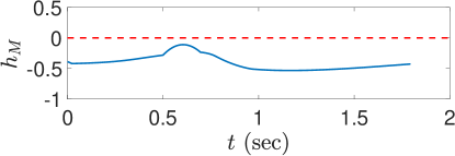
Figure 11: Pointwise maximum $h_{M}=\max\{h_{ij},h_{1},h_{2},h_{\theta}\}$ for the two agents.

We choose $u_{M}=2,\omega_{M}=5,T=2,\mu=5$, so that $\gamma_{1}=1.2,\gamma_{2}=0.8,\alpha_{1}=\alpha_{2}=\frac{5\pi}{4}$. The safety distance is chosen as $d_{m}=0.1$. Figure 10 plots the closed-loop trajectories of the agent and shows that the agent visit the required sets, while remaining inside the safe region and maintaining the safe distance with each other at all times. This is also evident from Figure 11, where the pointwise maximum of all the barrier functions (i.e., $h_{ij},h_{1},h_{2},h_{\theta}$) is plotted. Since $h_{M}<0$ at all times, it implies that the both agents satisfy the safety requirements at all times.

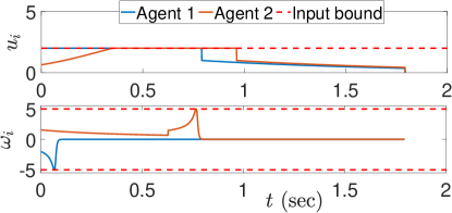
Figure 12: Inputs $u_{i}$ and $\omega_{i}$ for the two agents.

Figure 12 plots the individual inputs of the two agents. It is evident from the figure that the input constraints for the agents are satisfied at all times. Furthermore, note that the linear speeds $u_{1},u_{2}$ go to zero before $t=2$, implying that the agents reach their respective goal sets within the user-defined time $T=2$.

Finally, we ran the single agent case (only Agent 1 is considered) for various values of the input bounds on the linear speed $u_{M}\in[0.02,0.1]$ and the required time of convergence $T\in[2,10]$ for 200 randomly chosen initial conditions $[x_{1}(0)\;y_{1}(0)]^{T}\notin C_{2}$. Figure 13 plots the value of $c$ such that the $c-$sublevel set of the Lyapunov function $V_{1}$ is a FxT-DoA for the system dynamics in (19). It can be seen that for a fixed value of $u_{M}$, the value of $c$ increases as the required time of convergence increases (see the solid lines in the figure). Furthermore, it can be observed that for a given value of the required time of convergence $T$, the value of $c$ increases as the input bound $u_{M}$ increases (see the dotted vertical lines in the figure). This demonstrates that the domain of attraction for fixed-time stability expands if $T$ or $u_{M}$ increases, as discussed in Section 4.3.

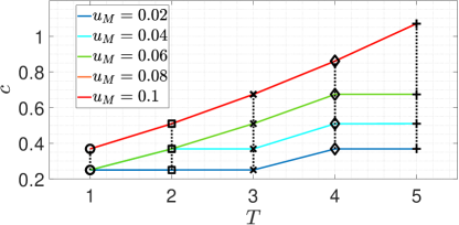
Figure 13: The value of $c$ such that $D=\{x\;|\;V_{1}(x)\leq c\}$ is the FxT-DoA for various values of $u_{M}$ and $T$.

7 Conclusions

In this paper, we considered the problem of satisfying spatiotemporal constraints requiring that the closed-loop trajectories of a class of nonlinear, control-affine systems remain in a safe set at all times, and reach a goal set within a fixed time in the presence of control input constraints. We established the relation between the domain of attraction for fixed-time stability, the input bounds and the time of convergence, showing that relaxing the time constraint or increasing the input bound results into a larger FxT-DoA. Then, we proposed a novel QP formulation, proved its feasibility under the assumption of existence of a control input that renders the safe set forward invariant, and showed continuity of the solution of the proposed QP. In the future, we would like to study the spatiotemporal control synthesis for large-scale multi-agent systems with concurrent consideration of switching in the dynamics or the system states. It will be interesting to see how the proposed method extends to systems with non-smooth dynamics, and how to formulate efficient optimization methods under such spatiotemporal constraints.

Appendix A Proof of Lemma 5

Intuitively, for given control input bounds, a larger value of $T_{ud}$ (which results into smaller values of $\alpha_{1},\alpha_{2}$), i.e., relaxation of time of convergence, should result in satisfaction of (13c) with smaller value of $\delta_{1}$. Conversely, for a given $T_{ud}$ (and thus, for a given pair $\alpha_{1},\alpha_{2}$), a larger control authority should result into satisfaction of (13c) with smaller $\delta_{1}$. In order to verify the intuition , we can compute the closed-form solution of (13) for the case when the control input constraint is active, and see how the parameters $T_{ud},u_{m},u_{M}$ affect the optimal value of $\delta_{1}$. To this end, consider the Lagrangian of the QP in (13):

$$\begin{split}L\coloneqq&\frac{1}{2}u^{2}+\frac{1}{2}\delta_{1}^{2}+c\delta_{1}+\lambda_{2}(u-u_{M})+\lambda_{3}(u_{m}-u)\\ &+\lambda_{1}(L_{f}V+L_{g}V(x)u-\delta_{1}V+\alpha_{1}V^{\gamma_{1}}+\alpha_{2}V^{\gamma_{2}}).\end{split}$$ (22)

Now, in order to see the effect of how input constraints affect $\delta_{1}$, the case when the constraint $u=u_{M}$ is active is studied under the assumption that $u_{M}>0$. Lemma 4 guarantees feasibility of the QP in (13) for all $x\notin S_{G}$. Thus, the Slater’s condition holds and the KKT conditions are both necessary and sufficient for optimality (see e.g., [7, Chapter 5]). Using the KKT conditions, it follows that the optimal solution $(u^{\star},\delta_{1}^{\star},\lambda_{1}^{\star},\lambda_{2}^{\star},\lambda_{3}^{\star})$ satisfies

$$\delta_{1}^{\star}(x) =-c+\lambda_{1}^{\star}(x)V(x),$$

$$u^{\star}(x) =-\lambda_{2}^{\star}(x)+\lambda_{3}^{\star}(x)-\lambda_{1}^{\star}(x)L_{g}V(x),$$

$$\lambda_{1}^{\star}(x) \geq 0,\quad\lambda_{2}^{\star}(x)\geq 0,\quad\lambda_{3}^{\star}(x)\geq 0,$$

for any $x\notin S_{G}$. We are now ready to present the proof of Lemma 5.

For $u^{\star}(x)=u_{M}$, it is required that $\lambda_{2}^{\star}(x)>0$. Since $u^{\star}(x)=u_{M}$ and $u_{m}<u_{M}$, it follows that $u^{\star}(x)>u_{m}$ (i.e., the lower-bound constraint is inactive) and so $\lambda_{3}^{\star}(x)=0$. It follows that $\lambda_{2}^{\star}(x)=-u_{M}-\lambda_{1}^{\star}(x)L_{g}V(x)$.

Since $u^{\star}(x)=u_{M}$, the constraint (13c) must be active. Otherwise, we have $\lambda_{1}^{\star}(x)=0$, which implies that $\lambda_{2}^{\star}(x)=-u_{M}<0$, which violates the optimality condition $\lambda_{2}^{\star}(x)\geq 0$. Thus, for $\lambda_{1}^{\star}(x)>0$ when $u^{\star}(x)=u_{M}$, it is essential that the constraint (13c) is active, and it follows that the optimal value of $\delta_{1}$ is given as:

$$\delta_{1}^{\star}(x)= \frac{L_{f}V(x)+L_{g}V(x)u_{M}+\alpha_{1}V(x)^{\gamma_{1}}+\alpha_{2}V(x)^{\gamma_{2}}}{V(x)}$$

$$= \frac{L_{f}V(x)+L_{g}V(x)u_{M}}{V(x)}+\alpha_{1}V(x)^{\gamma_{1}-1}+\alpha_{2}V(x)^{\gamma_{2}-1}.$$

Using this, and the definition of function $a(x)$, it follows that

$$\lambda_{1}^{\star}(x)=\frac{a(x)}{V(x)^{2}},\quad\lambda_{2}^{\star}(x)=-u_{m}-L_{g}V(x)\frac{a(x)}{V(x)^{2}}.$$

Now, for $x\in S_{M}$, it holds that $\lambda_{1}^{\star}(x)>0$ and $\lambda_{2}^{\star}(x)>0$ and thus, the optimal value of $\delta_{1}$ is given by (15) and that the optimal value of $u$ being $u^{\star}=u_{M}$ holds when $x\in S_{M}$.

Appendix B Proof of Theorem 1

The proof is based on [23, Theorem 2.1]. Denote by $I(x)$, the indices of rows of matrix $A(x)$ corresponding to the active constraints, i.e., $j\in I(x)$ implies $A_{j}(x)z^{\star}(x)=b_{j}(x)$, where $A_{j}\in\mathbb{R}^{1\times m+2}$ is the $j$-th row of the matrix $A$ and $b_{j}\in\mathbb{R}$ the $j$-th element of $b$. Define matrix $A_{ac}$ and $b_{ac}$ by collecting $A_{j}(x)$, and of $b_{j}$, respectively, so that $A_{ac}(x)z^{\star}(x)=b_{ac}(x)$. Since at most one of the input constraints $u_{i}\leq u_{M_{i}}$ or $u_{m_{i}}\leq u_{i}$ can be active at any given time, the matrix $A_{ac}(x)$ has $k$ rows from $\begin{bmatrix}A_{u}&\mathbf{0}_{2m}&\mathbf{0}_{2m}\end{bmatrix}$, where $k\leq m$, which are linearly independent. Furthermore, it has $p$ rows from $\begin{bmatrix}L_{g}h_{G}&-h_{G}&0\\ L_{g}h_{S}&0&h_{S}\end{bmatrix}$, where $p\leq 2$. Since $h_{G},h_{S}\neq 0$ for $x\in\textnormal{int}(S_{S})\setminus S_{G}$, these $k+p$ rows are linearly independent. Thus, the matrix $A_{ac}$ is full row-rank, i.e., the gradients of the active constraints $\{A_{ac_{i}}(x)\}$, where $A_{ac_{i}}(x)$ is the $i-$th row of matrix $A_{ac}(x)$, are linearly independent.

The second derivative $\nabla_{zz}L$ of the Lagrangian defined as

$$L(z,x,\lambda)\coloneqq\frac{1}{2}z^{T}Hz+F^{T}z+\lambda^{T}(A(x)z-b(x)),$$

with respect to $z$ is $H$, which is a positive definite matrix. Using this, and the fact that the QP (17) is feasible, it holds that the second-order sufficient conditions for optimality hold (see e.g. [23, Section 2.3]). Note that [23, Theorem 2.1] requires that the objective function and the functions $G_{i}(x,u)$ have the second derivatives jointly continuous in $(x,u)$. Since the objective function $\frac{1}{2}z^{T}Hz+F^{T}z$ is independent of $x$, and the constraint functions $G_{i}(x,u)$ are linear in $u$, the second derivative of these functions are independent of $x$, and thus, satisfy this condition trivially. Finally, the strict complementary slackness condition is satisfied per Assumption 3. Thus, all the conditions of [23, Theorem 2.1] are satisfied. Therefore, for every $x\in\textnormal{int}(S_{S})\setminus S_{G}$, there exists an open neighborhood $\mathcal{X}\subset\textnormal{int}(S_{S})\setminus S_{G}$ of $x$ such that the solution $z^{\star}(x)$ is continuous for all $x\in\mathcal{X}$. Since this holds for all $x\in\textnormal{int}(S_{S})\setminus S_{G}$, it follows that the solution $z^{\star}(x)$ is continuous for all $x\in\textnormal{int}(S_{S})\setminus S_{G}$.

References

- [1] Ravi P Agarwal and V Lakshmikantham. Uniqueness and Non-uniqueness Criteria for Ordinary Differential Equations, volume 6. World Scientific, 1993.
- [2] Aaron D Ames, Kevin Galloway, Koushil Sreenath, and Jessy W Grizzle. Rapidly exponentially stabilizing control Lyapunov functions and hybrid zero dynamics. IEEE Transactions on Automatic Control, 59(4):876–891, 2014.
- [3] Aaron D Ames, Xiangru Xu, Jessy W Grizzle, and Paulo Tabuada. Control barrier function based quadratic programs for safety critical systems. IEEE Transactions on Automatic Control, 62(8):3861–3876, 2017.
- [4] J-P Aubin and Arrigo Cellina. Differential Inclusions: Set-valued Maps and Viability Theory, volume 264. Springer Science & Business Media, 2012.
- [5] Sanjay P Bhat and Dennis S Bernstein. Finite-time stability of continuous autonomous systems. SIAM Journal on Control and Optimization, 38(3):751–766, 2000.
- [6] Franco Blanchini. Set invariance in control. Automatica, 35(11):1747–1767, 1999.
- [7] Stephen Boyd and Lieven Vandenberghe. Convex Optimization. Cambridge university press, 2004.
- [8] Anthony V Fiacco. Sensitivity analysis for nonlinear programming using penalty methods. Mathematical Programming, 10(1):287–311, 1976.
- [9] Kunal Garg and Dimitra Panagou. Control-Lyapunov and control-barrier functions based quadratic program for spatio-temporal specifications. In 58th IEEE Conference on Decision and Control, pages 1422–1429. IEEE, Dec 2019.
- [10] Kunal Garg and Dimitra Panagou. Characterization of domain of fixed-time stability under control input constraints. In Annual American Control Conference, pages 2268–2273, 2021.
- [11] Paul Glotfelter, Jorge Cortés, and Magnus Egerstedt. Nonsmooth barrier functions with applications to multi-robot systems. IEEE Control Systems Letters, 1(2):310–315, 2017.
- [12] Paul Glotfelter, Jorge Cortés, and Magnus Egerstedt. Boolean composability of constraints and control synthesis for multi-robot systems via nonsmooth control barrier functions. In 2018 IEEE Conference on Control Technology and Applications (CCTA), pages 897–902. IEEE, 2018.
- [13] Alexandra Grancharova, Esten Ingar Grøtli, Dac-Tu Ho, and Tor Arne Johansen. UAVs trajectory planning by distributed MPC under radio communication path loss constraints. Journal of Intelligent & Robotic Systems, 79(1):115–134, 2015.
- [14] Anqi Li, Li Wang, Pietro Pierpaoli, and Magnus Egerstedt. Formally correct composition of coordinated behaviors using control barrier certificates. In IEEE/RSJ International Conference on Intelligent Robots and Systems, pages 3723–3729. IEEE, 2018.
- [15] Yuchun Li and Ricardo G Sanfelice. Finite-time stability of sets for hybrid dynamical systems. Automatica, 100:200–211, 2019.
- [16] Lars Lindemann and Dimos V Dimarogonas. Control barrier functions for signal temporal logic tasks. IEEE Control Systems Letters, 3(1):96–101, 2019.
- [17] Francisco Lopez-Ramirez, Denis Efimov, Andrey Polyakov, and Wilfrid Perruquetti. Conditions for fixed-time stability and stabilization of continuous autonomous systems. Systems & Control Letters, 129:26–35, 2019.
- [18] Benjamin J Morris, Matthew J Powell, and Aaron D Ames. Continuity and smoothness properties of nonlinear optimization-based feedback controllers. In 54th IEEE Conference on Decision and Control, pages 151–158. IEEE, 2015.
- [19] Quan Nguyen and Koushil Sreenath. Exponential control barrier functions for enforcing high relative-degree safety-critical constraints. In 2016 American Control Conference, pages 322–328, 2016.
- [20] Sergey Parsegov, Andrey Polyakov, and Pavel Shcherbakov. Nonlinear fixed-time control protocol for uniform allocation of agents on a segment. In 51st Conference on Decision and Control, pages 7732–7737. IEEE, 2012.
- [21] Andrey Polyakov. Nonlinear feedback design for fixed-time stabilization of linear control systems. IEEE Transactions on Automatic Control, 57(8):2106, 2012.
- [22] Manuel Rauscher, Melanie Kimmel, and Sandra Hirche. Constrained robot control using control barrier functions. In IEEE/RSJ International Conference on Intelligent Robots and Systems, pages 279–285. IEEE, 2016.
- [23] Stephen M Robinson. Perturbed Kuhn-Tucker points and rates of convergence for a class of nonlinear-programming algorithms. Mathematical Programming, 7(1):1–16, 1974.
- [24] Muhammad Zakiyullah Romdlony and Bayu Jayawardhana. Stabilization with guaranteed safety using control Lyapunov-barrier function. Automatica, 66:39–47, 2016.
- [25] Martin Saska, Zdenek Kasl, and Libor Přeucil. Motion planning and control of formations of micro aerial vehicles. IFAC Proceedings Volumes, 47(3):1228–1233, 2014.
- [26] W. Shaw Cortez, D. Oetomo, C. Manzie, and P. Choong. Control barrier functions for mechanical systems: Theory and application to robotic grasping. IEEE Transactions on Control Systems Technology, pages 1–16, 2019.
- [27] Mohit Srinivasan, Samuel Coogan, and Magnus Egerstedt. Control of multi-agent systems with finite time control barrier certificates and temporal logic. In 57th IEEE Conference on Decision and Control, pages 1991–1996. IEEE, 2018.
- [28] Keng Peng Tee, Shuzhi Sam Ge, and Eng Hock Tay. Barrier Lyapunov functions for the control of output-constrained nonlinear systems. Automatica, 45(4):918–927, 2009.
- [29] James Usevitch, Kunal Garg, and Dimitra Panagou. Strong invariance using control barrier functions: A Clarke tangent cone approach. In 59th Conference on Decision and Control, pages 2044–2049. IEEE, Dec 2020.
- [30] Li Wang, Aaron Ames, and Magnus Egerstedt. Safety barrier certificates for heterogeneous multi-robot systems. In American Control Conference, pages 5213–5218. IEEE, 2016.
- [31] Li Wang, Aaron Ames, and Magnus Egerstedt. Safety barrier certificates for collisions-free multirobot systems. IEEE Transactions on Robotics, 33(3):661–674, 2017.
- [32] Xiangru Xu, Paulo Tabuada, Jessy W Grizzle, and Aaron D Ames. Robustness of control barrier functions for safety critical control. IFAC-PapersOnLine, 48(27):54–61, 2015.