First-passage percolation in random planar maps
and Tutte’s bijection

Abstract

We consider large random planar maps and study the first-passage percolation distance obtained by assigning independent identically distributed lengths to the edges. We consider the cases of quadrangulations and of general planar maps. In both cases, the first-passage percolation distance is shown to behave in large scales like a constant times the usual graph distance. We apply our method to the metric properties of the classical Tutte bijection between quadrangulations with $n$ faces and general planar maps with $n$ edges. We prove that the respective graph distances on the quadrangulation and on the associated general planar map are in large scales equivalent when $n\to\infty$.

1 Introduction

A planar map is a finite planar graph embedded in the sphere and considered up to orientation-preserving homeomorphisms. In this work, we only consider rooted planar maps, meaning that we distinguish an oriented edge called the root edge, whose origin is the root vertex. There exist many different models of random maps depending on the conditions one imposes on the degrees of faces, the existence or non-existence of multiple edges and loops, etc. In the following, we always allow loops and multiple edges. A particular case that will play a central role in this article is the case of quadrangulations, where all faces have degree $4$. For any map $M$, we denote its vertex set by $V(M)$ and the graph distance on the map $M$ by $\mathrm{d}_{\mathrm{gr}}^{M}$. The root vertex is usually denoted by $\rho$.

Several recent developments (see in particular [1, 2, 3, 14, 18]) have established that, for a wide range of models of random maps, the vertex set viewed as a metric space for the (suitably rescaled) graph distance, converges in distribution when the size of the map tends to infinity towards a random compact metric space called the Brownian map. This convergence holds in the sense of the Gromov-Hausdorff convergence for compact metric spaces. The convergence to the Brownian map gives a unified approach to asymptotic properties of different models of random planar maps.

A natural question is to ask what can be said when the graph distance is replaced by other choices of distances on the vertex set $V(M)$. A simple way to get other distances is to assign positive weights (or lengths) to the edges: The distance between two vertices will then be the minimal total weight of a path connecting these two vertices. When the weights of the different edges are chosen to be independent and identically distributed given the planar map $M$ in consideration, this leads to the so-called first-passage percolation distance, which we denote here by $\mathrm{d}_{\mathrm{fpp}}^{M}$. Of course, when weights are all equal to $1$ we recover the graph distance. The recent paper [6] has investigated the asymptotic properties of the first-passage percolation distance in large triangulations. Roughly speaking, the main results of [6] show that, in large scales, the first-passage percolation distance behaves like a constant times the graph distance. The relevant constant is found via a subadditivity argument and cannot be computed in general. Interestingly, this behavior for random planar maps is quite different from the one observed in deterministic lattices such as $\mathbb{Z}^{d}$, where the first-passage percolation distance is not believed to be asymptotically proportional to the graph distance (nor to the Euclidean distance).

One of the main goals of the present work is to show that results similar to those of [6] hold both for quadrangulations and for general planar maps. Recall that the diameter of a typical quadrangulation with $n$ faces, or of a typical planar map with $n$ edges is known to be of order $n^{1/4}$.

Theorem 1.

For every integer $n\geq 1$, let $Q_{n}$ be uniformly distributed over the set of all rooted quadrangulations with $n$ faces, and let $M_{n}$ be uniformly distributed over the set of all rooted planar maps with $n$ edges. Define the first-passage percolation distances $\mathrm{d}_{\mathrm{fpp}}^{Q_{n}}$ and $\mathrm{d}_{\mathrm{fpp}}^{M_{n}}$ by assigning independent and identically distributed weights to the edges of $Q_{n}$ and $M_{n}$. Assume that the common distribution of the weights is supported on a compact subset of $(0,\infty)$. Then there exist two positive constants c and $\textbf{c}^{\prime}$ such that

$$n^{-1/4}\sup_{x,y\in V(Q_{n})}\left|\mathrm{d}_{\mathrm{fpp}}^{Q_{n}}(x,y)-\textbf{c}\,\mathrm{d}_{\mathrm{gr}}^{Q_{n}}(x,y)\right|\underset{n\to\infty}{\longrightarrow}0$$

and

$$n^{-1/4}\sup_{x,y\in V(M_{n})}\left|\mathrm{d}_{\mathrm{fpp}}^{M_{n}}(x,y)-\textbf{c}^{\prime}\mathrm{d}_{\mathrm{gr}}^{M_{n}}(x,y)\right|\underset{n\to\infty}{\longrightarrow}0$$

where both convergences hold in probability.

As an immediate consequence of the theorem, we get that the convergence to the Brownian map still holds for both models in consideration if the graph distance is replaced by the first-passage percolation distance. More precisely, under the assumptions of Theorem 1 and with the same constants c and $\textbf{c}^{\prime}$, we have

$$\left(V(Q_{n}),{\left(\frac{9}{8n}\right)}^{1/4}\mathrm{d}_{\mathrm{fpp}}^{Q_{n}}\right)\overset{\textrm{(d)}}{\underset{n\to\infty}{\longrightarrow}}({\text{m}_{\infty}},\textbf{c}\,D^{*}),$$ (1)

and

$$\left(V(M_{n}),{\left(\frac{9}{8n}\right)}^{1/4}\mathrm{d}_{\mathrm{fpp}}^{M_{n}}\right)\overset{\textrm{(d)}}{\underset{n\to\infty}{\longrightarrow}}({\text{m}_{\infty}},\textbf{c}^{\prime}D^{*}),$$ (2)

where $({\text{m}_{\infty}},D^{*})$ is the Brownian map, and both convergences hold in distribution in the Gromov-Hausdorff space. Indeed, this follows from Theorem 1 and the known convergences for the graph distance which have been established in [14, 18] for $Q_{n}$ and in [3] for $M_{n}$. It is remarkable that the same constant $(9/8)^{1/4}$ appears in both (1) and (2). This will be better understood in the next theorem.

Another major goal of the present article is to have a better understanding of the metric properties of Tutte’s bijection. Recall that Tutte’s bijection, also called the trivial bijection, gives for every $n\geq 1$ a one-to-one correspondence between the set of all rooted quadrangulations with $n$ faces and the set of all rooted planar maps with $n$ edges. The definition of this correspondence should be clear from Figure 1. The following theorem can be interpreted by saying that Tutte’s transformation acting on a large quadrangulation is nearly isometric with respect to the graph distances.

Theorem 2.

Let $Q_{n}$ be uniformly distributed over the set of all rooted quadrangulations with $n$ faces and let $M_{n}$ be the image of $Q_{n}$ under Tutte’s bijection, so that $M_{n}$ is uniformly distributed over the set of all rooted planar maps with $n$ edges and $V(M_{n})$ is identified to a subset of $V(Q_{n})$. Then,

$$n^{-1/4}\sup_{x,y\in V(M_{n})}\left|\mathrm{d}_{\mathrm{gr}}^{Q_{n}}(x,y)-\mathrm{d}_{\mathrm{gr}}^{M_{n}}(x,y)\right|\underset{n\to\infty}{\longrightarrow}0$$

where the convergence holds in probability.

We can combine Theorems 1 and 2 to get that, if $Q_{n}$ and $M_{n}$ are linked by Tutte’s bijection, the convergences in distribution (1) and (2) hold jointly, with the same space $({\text{m}_{\infty}},D^{*})$ in the limit. This is reminiscent of Theorem 1.1 in [3], which gives a similar joint convergence, but in the case where $Q_{n}$ and $M_{n}$ are linked by a different bijection (the Ambjørn-Budd bijection) which is more faithful to graph distances.

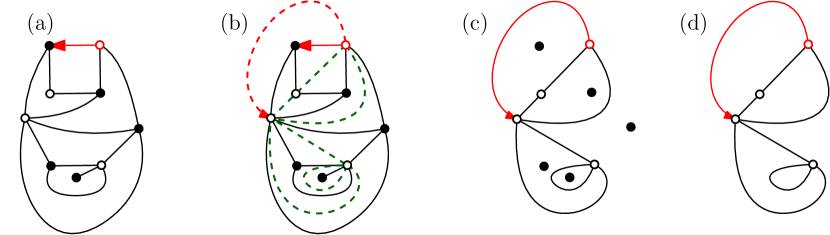
Figure 1: Illustration of Tutte’s bijection. (a) On the left, a quadrangulation with $7$ faces. Color the tail of its root vertex in white, and every other vertex in black and white so that adjacent vertices have a different color. (b) In every face of the quadrangulation, add a diagonal between its white corners. (c) Erase the edges of the quadrangulation. (d) The black vertices now have degree zero and are also erased. We obtain a map with $7$ edges, which is rooted at the edge corresponding to the diagonal drawn in the face to the right of the root edge of the quadrangulation, oriented so that the root vertex remains the same.

We can also give versions of the preceding results for the infinite random lattices that arise as local limits (in the Benjamini-Schramm sense) of large quadrangulations or general planar maps. We write $Q_{\infty}$ for the uipq or uniform infinite planar quadrangulation, and $M_{\infty}$ for the uipm or uniform infinite planar map. As was observed by Ménard and Nolin [17], the uipm can be obtained by applying (a generalized version of) Tutte’s correspondence to the uipq.

Theorem 3.

Let $\mathrm{d}_{\mathrm{fpp}}^{Q_{\infty}}$ and $\mathrm{d}_{\mathrm{fpp}}^{M_{\infty}}$ be the first-passage percolation distances defined on the vertex sets $V(Q_{\infty})$ and $V(M_{\infty})$, respectively, by assigning edge weights satisfying the same assumptions as in Theorem 1. Write $\rho_{Q_{\infty}}$ and $\rho_{M_{\infty}}$ for the respective root vertices of $Q_{\infty}$ and $M_{\infty}$. Then, for every $\varepsilon>0$,

$$\lim_{r\to\infty}\mathbb{P}\left(\sup_{x,y\in V(Q_{\infty}),\ \mathrm{d}_{\mathrm{gr}}^{Q_{\infty}}(\rho_{Q_{\infty}},x)\vee\mathrm{d}_{\mathrm{gr}}^{Q_{\infty}}(\rho_{Q_{\infty}},y)\leq r}|\mathrm{d}_{\mathrm{fpp}}^{Q_{\infty}}(x,y)-\textbf{c}\,\mathrm{d}_{\mathrm{gr}}^{Q_{\infty}}(x,y)|>\varepsilon r\right)=0,$$

and similarly,

$$\lim_{r\to\infty}\mathbb{P}\left(\sup_{x,y\in V(M_{\infty}),\ \mathrm{d}_{\mathrm{gr}}^{M_{\infty}}(\rho_{M_{\infty}},x)\vee\mathrm{d}_{\mathrm{gr}}^{M_{\infty}}(\rho_{M_{\infty}},y)\leq r}|\mathrm{d}_{\mathrm{fpp}}^{M_{\infty}}(x,y)-\textbf{c}^{\prime}\mathrm{d}_{\mathrm{gr}}^{M_{\infty}}(x,y)|>\varepsilon r\right)=0,$$

with the same constants c and $\textbf{c}^{\prime}$ as in Theorem 1. Moreover, if the uipq $Q_{\infty}$ and the uipm $M_{\infty}$ are linked by Tutte’s correspondence, we have also

$$\lim_{r\to\infty}\mathbb{P}\left(\sup_{x,y\in V(M_{\infty}),\ \mathrm{d}_{\mathrm{gr}}^{M_{\infty}}(\rho_{M_{\infty}},x)\vee\mathrm{d}_{\mathrm{gr}}^{M_{\infty}}(\rho_{M_{\infty}},y)\leq r}|\mathrm{d}_{\mathrm{gr}}^{M_{\infty}}(x,y)-\mathrm{d}_{\mathrm{gr}}^{Q_{\infty}}(x,y)|>\varepsilon r\right)=0.$$

A consequence of the first assertions of the theorem is the fact that balls (centered at the root vertex) for the first-passage percolation distance are asymptotically the same as for the graph distance, both in $Q_{\infty}$ and in $M_{\infty}$. More precisely, in $Q_{\infty}$ for definiteness, the (metric) ball of radius $r$ for the first-passage percolation distance will be contained in the graph distance ball of radius $(1+\varepsilon)r/\textbf{c}$ and will contain the graph distance ball of radius $(1-\varepsilon)r/\textbf{c}$, with high probability when $r$ is large. This is in sharp contrast with the behavior expected for deterministic lattices.

In the same way as in [6], our proofs rely on a “skeleton decomposition” which in the case of quadrangulations appeared first in the work of Krikun [10], and has been used extensively in [11]. Recall that, in the uipq $Q_{\infty}$, the hull of radius $r$ is defined as the complement of the infinite connected component of the complement of the ball of radius $r$ centered at the root vertex (informally, the hull is obtained by filling in the finite holes in the ball of radius $r$, see Section 2 for a more precise definition). The skeleton decomposition provides a detailed description of the joint distribution of layers of the uipq, where, roughly speaking, a layer corresponds to the part of the map between the boundary of the hull of radius $r$ and the boundary of the hull of radius $r+1$. This description allows us to compare the uipq near the boundary of a hull with another infinite model which we call the lhpq for lower half-plane quadrangulation (Section 3). The point is then that a subadditive ergodic theorem can be applied to evaluate first-passage percolation distances in the lhpq. Quite remarkably, this method carries over to the study of the first-passage percolation distance in the general planar maps that are obtained from quadrangulations by Tutte’s corrrespondence, with the minor difference that we must restrict to hulls of even radius in the quadrangulation.

Even though the idea of using the skeleton decomposition already appeared in [6] in the setting of triangulations, there are important differences between the present work and [6], and our proofs are by no means straightforward extensions of those of [6]. In particular, a very important ingredient of our method involves bounds on graph distances along the boundary in the lhpq. To derive these bounds we use a completely different approach from that developed in [6] for the model called the lower half-plane triangulation. Our approach, which relies on certain ideas of [4], is simpler and avoids the heavy combinatorial analysis of [6]. Similarly, the application of the subadditive ergodic theorem gives information about the first-passage percolation distance between points of the boundary of a hull of the uipq and the root vertex (Proposition 17 below) but a key step is then to derive information about the distance between a typical point and the root vertex in the finite quadrangulation $Q_{n}$ (Proposition 18): For this purpose, the lack of certain explicit combinatorial expressions did not allow us to use the same approach as in [6], and we had to develop a different method based on a coupling between $Q_{n}$ and the uipq. Finally, the treatment of a general planar map $M_{n}$ given as the image of the quadrangulation $Q_{n}$ under Tutte’s bijection also required a number of new tools, in particular because the graph distance on $M_{n}$ is not easily controlled in terms of the graph distance on $Q_{n}$.

The paper is organized as follows. Section 2 gives a number of preliminaries about planar maps and the skeleton decomposition. We introduce the notion of a quadrangulation of the cylinder, which already played an important role in [11], and we define the so-called truncated hulls, which are variants of the (standard) hulls considered in earlier work. Section 3 discusses the lower half-plane quadrangulation. In particular, we derive the important bounds controlling distances along the boundary (Proposition 8). Section 4 gives two technical propositions. The first one (Proposition 14) provides bounds for the distribution of the skeleton of a (truncated) hull of the uipq in terms of the skeleton associated with the lhpq. This is the key to transfer results obtained in the lhpq (by subadditive arguments) to the uipq. Section 5 derives our main results about first-passage percolation distances in quadrangulations. We start by proving Proposition 16, which estimates the $\mathrm{d}_{\mathrm{fpp}}^{Q_{\infty}}$-distance between a vertex of the boundary of the (truncated) hull of radius $r$ and the boundary of the hull of radius $r-{\left\lfloor\eta r\right\rfloor}$, for $\eta>0$ small. This key proposition is then used to get Proposition 17 concerning the distance between a point of the boundary of a hull and the root vertex. Then the hard work is to prove Proposition 18 controlling the distance between a uniformly distributed vertex of $Q_{n}$ and the root vertex. From this proposition, it is not too hard to derive Theorem 22, which gives the part of Theorem 1 dealing with quadrangulations. Section 6 contains certain technical results concerning graph distances in the general maps associated with quadrangulations via Tutte’s correspondence. We introduce the so-called downward paths, which are closely related to the skeleton decomposition of the associated quadrangulation, and we derive important bounds on the length of these paths (Lemma 25). Finally, Section 7 is devoted to the proof of the results concerning general maps. In particular, Theorem 34 shows that, if $M_{n}$ and $Q_{n}$ are linked by Tutte’s bijection, the first-passage percolation distance in $M_{n}$ is asymptotically proportional to the graph distance in $Q_{n}$. In the case where weights are equal to $1$, the proportionality constant has to be equal to $1$ (because of the known results about scaling limits of $Q_{n}$ and $M_{n}$), which gives Theorem 2 and then the part of Theorem 1 concerning general maps. Several proofs in this section are very similar to the proofs of Section 5. For this reason, we have only sketched certain arguments, but we emphasize the places where new ingredients are required.

2 Preliminaries

A (finite) planar map is a planar graph embedded in the sphere and seen up to orientation-preserving homeomorphisms. We allow multiple edges and loops. Since we consider only planar maps we often say map instead of planar map. If $M$ is a map, we denote the set of vertices, edges, and faces of $M$ by $V(M),E(M),F(M)$ respectively. We write $\mathrm{d}_{\mathrm{gr}}^{M}$ for the graph distance on $V(M)$. Given i.i.d. random weights $(\omega_{e})_{e\in E(M)}$ assigned to the edges of $M$, we also define the associated first-passage percolation distance $\mathrm{d}_{\mathrm{fpp}}^{M}$ as follows. We define the weight of a path $\gamma$ as the sum of the weights of its edges, and the first-passage percolation distance $\mathrm{d}_{\mathrm{fpp}}^{M}(x,y)$ between two vertices $x$ and $y$ of $M$ is the infimum of the weights of paths starting at $x$ and ending at $y$. Note that, if $\omega_{e}=1$ for every edge $e$, we recover the graph distance on $V(M)$.

A rooted map is a map with a distinguished oriented edge called the root edge. The tail of the root edge is called the root vertex and is usually denoted by $\rho$. The face lying to the right of the root edge is called the root face. We say that a rooted map is pointed if in addition it has a distinguished vertex $\partial$.

Models of quadrangulations.

A quadrangulation is a rooted map whose faces all have degree $4$. Quadrangulations are bipartite maps, so we may and will color the vertices of a quadrangulation in black and white so that two adjacent vertices have different colors and the root vertex is white.

A truncated quadrangulation is a rooted map such that

• the root face has a simple boundary and an arbitrary even degree,

• every edge incident to the root face is also incident to another face which has degree 3, and these triangular faces are distinct,

• all the other faces have degree 4.

The root face is also called the external face, and faces other than the external face are called inner faces. The length of the external boundary (the boundary of the external face) is called the perimeter of the truncated quadrangulation.

We will also consider infinite (rooted but not pointed) quadrangulations for which we assume — except in the case of the lhpq discussed in Section 3 — that they are embedded in the plane in such a way that all faces are bounded subsets of the plane, and furthermore every compact subset of the plane intersects only finitely many faces (and again infinite quadrangulations are viewed up to orientation preserving homeomorphisms). These properties hold a.s. for the uipq.

Hulls and truncated hulls.

Let $Q$ be a (finite or infinite) quadrangulation with root vertex $\rho$. For every integer $r\geq 1$, we denote the ball of radius $r$ in $Q$ by $B_{Q}(r)$. This ball is the map obtained by taking the union of all faces that are incident to a vertex at graph distance at most $r-1$ from $\rho$. Suppose in addition that $Q$ is finite and pointed, and let $R=\mathrm{d}_{\mathrm{gr}}^{Q}(\rho,\partial)$ be the graph distance between the root vertex and the distinguished vertex. Then for every integer $1\leq r\leq R-2$, the standard hull of radius $r$ of $Q$, denoted by $B^{\bullet}_{Q}(r)$, is the union of $B_{Q}(r)$ and of the connected components of its complement that do not contain $\partial$. If $Q$ is an infinite quadrangulation, then, for every $r\geq 1$, the standard hull of radius $r$ of $Q$ is defined as the union of $B_{Q}(r)$ and the finite connected components of its complement, and is also denoted by $B^{\bullet}_{Q}(r)$. In both the finite and the infinite case, the standard hull $B^{\bullet}_{Q}(r)$ is a quadrangulation with a simple boundary (meaning that all faces are quadrangles, except for one distinguished face, which has a simple boundary). If $r>1$ is not an integer, we will agree that $B_{Q}(r)=B_{Q}({\left\lfloor r\right\rfloor})$ and $B^{\bullet}_{Q}(r)=B^{\bullet}_{Q}({\left\lfloor r\right\rfloor})$.

We also need to define truncated hulls. To this end, consider first the case where $Q$ is finite and pointed. We label the vertices of $Q$ with their graph distance to $\rho$, and we consider an integer $r$ such that $0<r<\mathrm{d}_{\mathrm{gr}}^{Q}(\rho,\partial)$. Inside every face such that the labels of its incident corners are $r,r-1,r,r+1$, we draw a “diagonal” between the corners of label $r$. The added edges form a collection of cycles, from which we extract a “maximal” simple cycle $\partial_{r}Q$. This cycle is maximal in the sense that the connected component of the complement of $\partial_{r}Q$ that contains the distinguished vertex contains no vertex with label less than or equal to $r$. See [11, Section 2.2] for more details. The exterior of $\partial_{r}Q$ is the connected component of the complement of $\partial_{r}Q$ that contains the marked vertex of $Q$. If $Q$ is an infinite quadrangulation, the cycles $\partial_{r}Q$ can be defined in exactly the same way, now for every integer $r>0$ (the exterior of $\partial_{r}Q$ is now the the unbounded connected component of the complement of $\partial_{r}Q$).

In both the finite and the infinite case, the truncated hull of radius $r$ of $Q$ is the map $\mathcal{H}^{\text{tr}}_{Q}(r)$ made of $\partial_{r}Q$ and of the edges of $Q$ inside $\partial_{r}Q$, and is rooted at the “same” edge as $Q$. Then we may view $\mathcal{H}^{\text{tr}}_{Q}(r)$ as a truncated quadrangulation (for which the external face corresponds to the exterior of $\partial_{r}Q$) provided we re-root $\mathcal{H}^{\text{tr}}_{Q}(r)$ at an edge of its external boundary.

Quadrangulations of the cylinder.

A quadrangulation of the cylinder of height $R>0$ is a rooted map $Q$ with two distinguished faces, called the top and bottom faces (the other faces are called inner faces), such that

1. the boundary of the top (resp. bottom) face, called the top boundary (resp. the bottom boundary) is a simple cycle,

2. $Q$ is rooted at an oriented edge of its bottom boundary so that the bottom face lies on the right of the root edge (so the bottom face is the root face),

3. every edge of the top (resp. bottom) boundary is incident both to the top (resp. bottom) face and to a triangular face, these triangular faces are distinct, and all other inner faces have degree 4,

4. any vertex of the top boundary is at graph distance $R$ from the bottom boundary, and the inner triangular face incident to any edge of the top boundary is also incident to a vertex at graph distance $R-1$ from the bottom boundary.

Let $Q$ be a quadrangulation of the cylinder of height $R$. Label every vertex of $Q$ by its distance from the bottom boundary. For $0<r<R$ we can define $\partial_{r}Q$ and the truncated hull of radius $r$ in a way very similar to what we did for pointed quadrangulations ($\partial_{r}Q$ is the “maximal” cycle made of diagonals between corners labeled $r$ in faces whose corners are labeled $r-1,r,r+1,r$, and the exterior of $\partial_{r}Q$ now contains the top cycle). See [11, Section 2.3] for details. Note that the truncated hull of radius $r$ of $Q$ is itself a quadrangulation of the cylinder of height $r$. By convention, we agree that $\partial_{0}Q$ denotes the bottom boundary, and $\partial_{R}Q$ stands for the top boundary of $Q$. We will assume that quadrangulations of the cylinder are drawn in the plane in such a way that the top face is the unbounded face (see Figure 3). Then we will orient the cycles $\partial_{r}Q$ clockwise by convention.

Figure 2: We can split the root edge of a truncated hull, add a loop inside the newly created face, and see the map as a quadrangulation of the cylinder of bottom cycle the added loop.

We may view the truncated hull of radius $r$ of a pointed quadrangulation $Q$ as a quadrangulation of the cylinder of height $r$, by splitting the root edge of $Q$ into a double edge and adding a loop inside the newly created face as in Figure 2. In this way, we get a quadrangulation of the cylinder of height $r$ whose bottom cycle is a loop.

Left-most geodesics.

Let $Q$ be a quadrangulation of the cylinder of height $R$ and let $0<r\leq R$. We now explain a “canonical” choice of a geodesic between a vertex of $\partial_{r}Q$ and the bottom cycle $\partial_{0}Q$. So let $v$ be a vertex on $\partial_{r}Q$, and let $e$ be the edge of $\partial_{r}Q$ with tail $v$ (recall our convention for the orientation of $\partial_{r}Q$). Then list all edges incident to $v$ in clockwise order around $v$, starting from $e$. The first step of the left-most geodesic from $v$ to $\partial_{0}Q$ is the last edge in this enumeration that connects $v$ to $\partial_{r-1}Q$ (Property (iv) above ensures that there is at least one such edge). We define the next steps of the geodesic by the obvious induction.

Skeleton decomposition.

Let $Q$ be a quadrangulation of the cylinder of height $R$. Following ideas in [10], the article [11] gives a representation of $Q$ by a forest of planar trees of height at most $R$ and a collection of truncated quadrangulations indexed by the vertices of this forest. We refer to [11] for more details, and give a brief presentation.

We first add the edges of $\partial_{r}Q$ to $Q$ for every $0<r\leq R$ and recall that these edges are oriented clockwise in each cycle $\partial_{r}Q$. Let $0<r\leq R$, and let $e$ be an edge of $\partial_{r}Q$. Then $e$ is incident to exactly one triangular face in $Q$ whose third vertex is at distance $r-1$ from the bottom boundary. We call this face the downward triangle with top edge $e$. Furthermore, if $v$ is the aim of $e$, the downward triangle with top edge $e$ is also incident to the first edge of the left-most geodesic from $v$ to the bottom boundary.

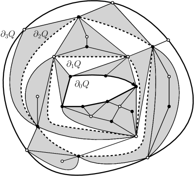
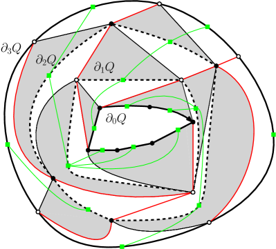
Figure 3: Left, a quadrangulation of the cylinder of height $3$, with its cycles $\partial_{1}Q$, $\partial_{2}Q$ in dashed lines. We always draw the top face as the infinite face. Downward triangles are in white and the slots in grey. Right, we erased the content of the slots; in green, the genealogical relation on edges of $\partial_{r}Q$ for $0\leq r\leq 3$, in red, the left-most geodesics to the bottom cycle follow the “right” side of downward triangles (assuming their top edge is “up”), or equivalently the “left” side of slots.

The downward triangles disconnect $Q$ into a collection of slots, which are filled in by finite maps with a simple boundary. See Figure 3. Any slot is contained in the region between $\partial_{r}Q$ and $\partial_{r-1}Q$ for some $1\leq r\leq R$, and there is a unique vertex $v$ of $\partial_{r}Q$ that is incident to the slot. We then say that the slot is associated with the edge of $\partial_{r}Q$ whose tail is $v$. We equip the set of edges of $\cup_{r=0}^{R}\partial_{r}Q$ with the following genealogical relation: for every $0<r\leq R$, an edge $e\in\partial_{r}Q$ is the parent of all the edges of $\partial_{r-1}Q$ that are incident to the slot associated with $e$, provided that this slot exists. See the right side of Figure 3.

We now explain how we can define the truncated quadrangulation associated with a slot, or rather with an edge $e\in\partial_{r}Q$, $1\leq r\leq R$. Suppose first that there is a slot associated with $e$. The part of $Q$ inside this slot, including its boundary, defines a planar map with a simple boundary and a distinguished vertex on this boundary. Adding one edge in the way explained in Figure 4 turns this map into a truncated quadrangulation $M$, which is rooted at the added edge as shown on Figure 4. If there is no slot associated with $e$ we let $M$ be the unique truncated quadrangulation with perimeter one and one inner face (rooted at its boundary edge so that the external face lies on the right of the root edge).

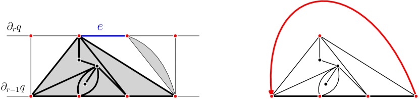
Figure 4: Left (in grey and thick black lines), the map with simple boundary filling the slot of an edge $e$ (in blue) of $\partial_{r}Q$ with $3$ offspring. Right, the truncated quadrangulation we obtain by adding a root edge “over the top vertex of the slot”.

Recalling the definition in [11], we say that a forest $\mathcal{F}$ with one marked vertex is $(R,p,q)$-admissible if

1. the forest consists of an ordered sequence of $q$ rooted plane trees,

2. these trees have height at most $R$,

3. exactly $p$ vertices of the forest are at height $R$,

4. the marked vertex is at height $R$ and belongs to the first tree.

Write $\mathbb{F}^{0}_{R,p,q}$ for the set of all $(R,p,q)$-admissible forests. We will also need the set of all forests with no marked vertex that satisfy properties (i) to (iii) above, and we denote this set by $\mathbb{F}_{R,p,q}$.

For $\mathcal{F}\in\mathbb{F}^{0}_{R,p,q}$ or $\mathcal{F}\in\mathbb{F}_{R,p,q}$ we let $\mathcal{F}^{*}$ denote the set of all vertices of $\mathcal{F}$ at height at most $R-1$. For every $e\in\mathcal{F}^{*}$, $c_{e}$ is the offspring number of $e$ in $\mathcal{F}$.

The construction described above and illustrated in Figure 3 provides a bijection that, with every quadrangulation $Q$ of the cylinder of height $R$, with top perimeter $q$ and bottom perimeter $p$, associates an $(R,p,q)$-admissible forest $\mathcal{F}$ and a collection $(S_{e})_{e\in\mathcal{F}^{*}}$ of truncated quadrangulations, such that $S_{e}$ has perimeter $c_{e}+1$ for every $e\in\mathcal{F}^{*}$. The forest encodes the genealogical relation of edges of $\cup_{r=0}^{R}\partial_{r}Q$: each tree in $\mathcal{F}$ corresponds to the descendants of an edge of the top boundary, the first tree is the one that contains the root edge, and the other trees are then listed by following the clockwise order on the top boundary. We call the forest $\mathcal{F}$ the skeleton of $Q$.

On the other hand, the union of all left-most geodesics forms a forest of trees made of edges of $Q$. This forest can be viewed as dual to the skeleton of $Q$, and the two forests do not cross, as suggested in Figure 3. This has the following important consequence. Let $v,w$ be two distinct vertices of the top boundary of $Q$, let $\mathcal{F}^{\prime}$ be the forest consisting of the trees of the skeleton that are rooted on the part of the top boundary between $v$ and $w$ (in clockwise order), and let $\mathcal{F}^{\prime\prime}$ consist of the other trees in the skeleton. Then for every $0\leq r<R$, the left-most geodesics from $v$ and $w$ coalesce before reaching $\partial_{r}Q$ or when hitting $\partial_{r}Q$ iff either $\mathcal{F}^{\prime}$ or $\mathcal{F}^{\prime\prime}$ has height strictly smaller than $R-r$.

Law of the skeleton decomposition of the UIPQ.

The following formulas are derived by singularity analysis from the generating series of truncated quadrangulations, computed in [10]. See [11, Section 2.5].

For every $1\leq p\leq n$, let $\mathbb{Q}^{\text{tr}}_{n,p}$ be the set of all truncated quadrangulations with a boundary of length $p$ and $n$ inner faces. There exists a sequence $(\kappa_{p})_{p\geq 1}$ of positive reals such that for every $p\geq 1$,

$$\#\mathbb{Q}^{\text{tr}}_{n,p}\underset{n\to\infty}{\sim}\kappa_{p}n^{-5/2}12^{-n}.$$

Furthermore,

$$\kappa_{p}\underset{p\to\infty}{\sim}\frac{64\sqrt{3}}{\pi\sqrt{2}}\sqrt{p}2^{-p}.$$ (3)

For every $p\geq 1$, we define

$$h(p) \overset{\text{def}}{=}\frac{1}{p}2^{p}\kappa_{p},$$

$$Z(p) \overset{\text{def}}{=}\sum_{n=p}^{\infty}\#\mathbb{Q}^{\text{tr}}_{n,p}12^{-n},$$

and we define the Boltzmann probability measure $\Gamma_{p}$ on $\cup_{n=p}^{\infty}\mathbb{Q}^{\text{tr}}_{n,p}$ by setting

$$\Gamma_{p}(Q)\overset{\text{def}}{=}\frac{12^{-n}}{Z(p)}.$$

for every $Q\in\mathbb{Q}^{\text{tr}}_{n,p}$, $n\geq p$. We also set, for every $p\geq 0$,

$$\theta(p) \overset{\text{def}}{=}6\cdot 2^{p}Z(p+1).$$

Then [11, Lemma 6], $(\theta(p))_{p\geq 0}$ is a critical offspring distribution with generating function

$$g_{\theta}(y)=1-\frac{8}{\left(\sqrt{\frac{9-y}{1-y}}+2\right)^{2}-1}.$$

Let $g^{(p)}_{\theta}=g_{\theta}\circ\cdots\circ g_{\theta}$ denote the $p$-th iterate of $g_{\theta}$. If $(Y_{p})_{p\geq 0}$ is a Bienaymé-Galton-Watson process with offspring distribution $\theta$ started at $Y_{0}=1$, then for every $p\geq 0$,

$$\mathbb{E}\left[y^{Y_{p}}\right]=g_{\theta}^{(p)}(y)=1-\frac{8}{\left(\sqrt{\frac{9-y}{1-y}}+2p\right)^{2}-1},\quad 0\leq y<1.$$

We now consider the uniform infinite planar quadrangulation $Q_{\infty}$ to which we can apply the preceding definition to get the cycles $\partial_{r}Q_{\infty}$ for every $r\geq 0$ (when $r=0$ we split the root edge as explained in Figure 2). For $r\geq 1$, we distinguish the edge of $\partial_{r}Q_{\infty}$ that corresponds to the first tree of the skeleton of the truncated hull of radius $r$, viewed as a quadrangulation of the cylinder of height $r$. Then, for every $0\leq r<s$ we define the annulus $\mathcal{C}(r,s)$ as the quadrangulation of the cylinder of height $s-r$ that corresponds to the part of $Q_{\infty}$ between $\partial_{r}Q_{\infty}$ and $\partial_{s}Q_{\infty}$, rooted at the distinguished edge of $\partial_{r}Q_{\infty}$.

Let $(\mathcal{F}^{0}_{r,s},(S_{e})_{e\in{\mathcal{F}^{0*}_{r,s}}})$ be the skeleton decomposition of $\mathcal{C}(r,s)$. Conditionally on the skeleton $\mathcal{F}_{r,s}^{0}$, the truncated quadrangulations $S_{e}$, $e\in\mathcal{F}_{r,s}^{0,*}$, are independent and the conditional distribution of $S_{e}$ is $\Gamma_{c_{e}+1}$, where we recall that $c_{e}$ is the number of offspring of $e$ in $\mathcal{F}_{r,s}^{0}$. See [11, Corollary 8].

Let $H_{r}$ be the length of $\partial_{r}Q_{\infty}$.

Proposition 4 ([11], Proposition 11).

For every $r\geq 1$ and $p\geq 1$,

$$\mathbb{P}(H_{r}=p)=K_{r}\kappa_{p}(2\pi_{r})^{p},$$ (4)

where

$$\pi_{r}=g_{\theta}^{(r)}(0)=1-\frac{8}{(3+2r)^{2}-1}$$ (5)

is the probability that a Bienaymé-Galton-Watson process of offspring distribution $\theta$ started at $1$ becomes extinct before generation $r$, and

$$K_{r}=\frac{32}{3\kappa_{1}}\frac{3+2r}{((3+2r)^{2}-1)^{2}}.$$

Consequently, we can find positive constants $M_{1},M_{2}$ and $\rho$ such that for every $a>0$ and $r\geq 1$,

$$\mathbb{P}(H_{r}\geq ar^{2}) \leq M_{1}e^{-\rho a},$$

$$\mathbb{P}(H_{r}\leq ar^{2}) \leq M_{2}a^{3/2}.$$

From the skeleton $\mathcal{F}_{r,s}^{0}$, we define a new forest $\mathcal{F}_{r,s}$ by “forgetting” the marked vertex and applying a uniform random circular permutation to the trees of $\mathcal{F}_{r,s}^{0}$. Then $\mathcal{F}_{r,s}$ is a random element of $\cup_{p\geq 1,q\geq 1}\mathbb{F}_{s-r,p,q}$.

Proposition 5 ([11], Corollary 10).

Let $p\geq 1$. The conditional distribution of $\mathcal{F}_{r,s}$ knowing that $H_{r}=p$ is as follows: for every $q>0$, for every $\mathcal{F}\in\mathbb{F}_{s-r,p,q}$,

$$\mathbb{P}\left(\mathcal{F}_{r,s}=\mathcal{F}\ |\ H_{r}=p\right)=\frac{h(q)}{h(p)}\prod_{e\in\mathcal{F}^{*}}\theta(c_{e}).$$ (6)

Proposition 6.

Let $q\geq 1$. The conditional distribution of $\mathcal{F}_{r,s}$ knowing that $H_{s}=q$ is as follows: for every $p>0$, for every $\mathcal{F}\in\mathbb{F}_{s-r,p,q}$,

$$\mathbb{P}\left(\mathcal{F}_{r,s}=\mathcal{F}\ |\ H_{s}=q\right)=\frac{\varphi_{r}(p)}{\varphi_{s}(q)}\prod_{e\in\mathcal{F}^{*}}\theta(c_{e}),$$ (7)

where

$$\varphi_{r}(p)=\frac{64}{3}p\frac{3+2r}{((3+2r)^{2}-1)^{2}}\pi_{r}^{p-1}.$$ (8)

We refer to formulas (18) and (19) in [11] for the last proposition.

3 The lower half-plane quadrangulation

3.1 Definition of the model

We construct an infinite quadrangulation with an infinite truncated boundary, which will be denoted by $\mathcal{L}$ and called the lower half plane quadrangulation or lhpq. Roughly speaking, $\mathcal{L}$ is what we see near a uniformly chosen random edge of the boundary of a very large truncated hull of $Q_{\infty}$ (see Proposition 7 below for a more precise statement). Our construction relies on the skeleton decomposition.

It will be convenient to use a particular embedding of $\mathcal{L}$ in the plane (see Figure 5). In the rest of this paper, we denote the set of non-negative integers by $\mathbb{N}$, and the set of non-positive integers by $-\mathbb{N}=\{0,-1,-2,...\}$. Every point of $\mathbb{Z}\times-\mathbb{N}$ will be a vertex of $\mathcal{L}$; the edges of the form $((i,0),(i+1,0))$ for $i\in\mathbb{Z}$ will be the edges of the boundary of $\mathcal{L}$; and the upper half-plane will correspond to an “external face” of $\mathcal{L}$. Furthermore, $\mathcal{L}$ will be rooted at the edge $((0,0),(1,0))$.

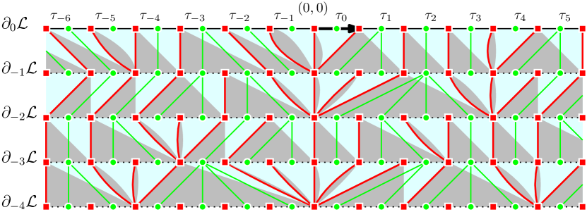
Figure 5: Embedding of the lhpq and its skeleton. The vertices of the lattice $\mathbb{Z}\times-\mathbb{N}$ are the red dots, the vertices of the forest are the green dots, the trees are drawn in green. We drew the downward triangles in cyan, and the slots in grey. Notice that the slot associated with an edge having no offspring may be empty though it is represented here as the “inside” of a double edge (this simply means that this double edge may be glued to form a single edge).
In red, left-most geodesics in the lhpq, named so because they follow the left-most edge going downward. They follow the left side of slots, or the right side of downward triangles. The left-most geodesics form the dual tree of the skeleton.

In order to construct $\mathcal{L}$, we start from a forest $(\tau_{i})_{i\in\mathbb{Z}}$ of i.i.d. Bienaymé-Galton-Watson trees with offspring distribution $\theta$ (as usual these trees are random plane trees). This forest will be the skeleton of the lhpq. A.s. each generation has an infinite number of individuals: we can thus embed vertices of the skeleton at generation $r\geq 0$ bijectively on $\{(j+\frac{1}{2},-r),j\in\mathbb{Z}\}$, in a way that is consistent with the order on vertices at generation $r$ of the forest, so that vertices in trees with non-negative indices $(\tau_{i})_{i\geq 0}$ fill the lower right quadrant $(1/2,0)+(\mathbb{N}\times-\mathbb{N})$, and vertices in trees with negative indices $(\tau_{i})_{i<0}$ fill the lower left quadrant $(-1/2,0)+(-\mathbb{N}\times-\mathbb{N})$. In particular the root of $\tau_{i}$ will be $(i+1/2,0)$. See the green trees on Figure 5. In what follows, we identify vertices of the skeleton and the points where they are embedded.

We denote by $\partial_{-r}\mathcal{L}$ the infinite line $\mathbb{Z}\times\{-r\}$ viewed as a linear graph. The skeleton of $\mathcal{L}$ induces a genealogical relation on the edges of $\cup_{r\geq 0}\partial_{-r}\mathcal{L}$, if we identify each edge with its middle point.

To each edge $e$ of $\partial_{-r}\mathcal{L}$, we associate a downward triangle with “top boundary” $e$ and “bottom vertex” the vertex $v$ of $\partial_{-r-1}\mathcal{L}$, chosen as follows. If $e$ has at least one offspring, then $v$ is the right-most vertex of the edge which is the right-most offspring of $e$. If not, let $e^{\prime}$ be the first edge of $\partial_{r}\mathcal{L}$ on the left of $e$ having at least one offspring. Then the downward triangles of $e$ and $e^{\prime}$ have the same bottom vertex.

Downward triangles delimit a collection of slots (see Figure 5), and each slot is associated with an edge of $\cup_{r\geq 0}\partial_{-r}\mathcal{L}$ as in the uipq. By construction, the edges of the lower boundary of a slot are exactly the offspring of the associated edge. The last step to get the lhpq is to fill in the slots, and we do so exactly as in the uipq, see Figure 6. We note that, for $r>0$, edges of $\partial_{-r}\mathcal{L}$ do not belong to $\mathcal{L}$: these edges are removed in order to get quadrangles by the gluing of two triangles.

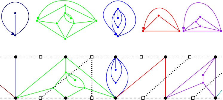
Figure 6: Constructing a part of the lhpq from truncated quadrangulations. In the lower part, the dotted lines are trees of the skeleton and the dashed lines are $\partial_{-r-1}\mathcal{L}$ and $\partial_{-r}\mathcal{L}$ for some $r\geq 0$. The upper part of the figure shows 5 truncated quadrangulations that fill in successive slots as shown in the lower part. Note that any edge of a truncated quadrangulation that is glued to some edge of $\partial_{-r}\mathcal{L}$ is removed in the lhpq.

Left-most geodesics in $\mathcal{L}$ are defined as in the case of quadrangulations of the cylinder, but are now infinite paths on $\mathcal{L}$ that start at a vertex of $\partial_{-r}\mathcal{L}$ and then visit each line $\partial_{-r^{\prime}}\mathcal{L}$, $r^{\prime}\geq r$, exactly once. Left-most geodesics form a forest whose vertex set is the lattice $\mathbb{Z}\times-\mathbb{N}$. This forest and the skeleton never intersect and can be seen as “dual” to each other. Furthermore, the two left-most geodesics started at $(i,0)$ and $(i^{\prime},0)$ with $i<i^{\prime}$ coalesce before height $j<0$ or exactly at height $j$ if and only if every $\tau_{k}$ with $i<k+\frac{1}{2}<i^{\prime}$ becomes extinct before generation $-j$. See Figure 5 for an illustration.

Note that the left-most geodesic started from any point $(i,0)$ of the top boundary breaks the lhpq into two halves. Any path whose endpoints are on different sides of this geodesic must cross it through one of its vertices. Note finally that left-most geodesics never cross any tree of the skeleton. As an example, the left-most geodesic started from $(0,0)$ is the vertical line $((0,-n))_{n\geq 0}$.

As another useful observation, we note that the graph distance between any point of $\partial_{r}\mathcal{L}$ and $\partial_{r^{\prime}}\mathcal{L}$ (with $r^{\prime}<r$) is exactly $r-r^{\prime}$.

3.2 The lower-half plane quadrangulation is the local limit of large hulls

The following proposition explains why we consider the model of the lhpq.

Proposition 7.

For every $r>0$, let $\mathcal{H}_{r}$ be the truncated hull of radius $r$ of the uipq, re-rooted at a uniformly chosen edge of its boundary. Then

$$\mathcal{H}_{r}\overset{\textrm{(d)}}{\underset{r\to\infty}{\longrightarrow}}\mathcal{L}$$

for the local topology on rooted planar maps.

We omit the proof as we will not need this result in the remaining part of the paper. See Proposition 7 in [6] for the analogous statement in the case of triangulations.

3.3 Control of distances along the boundary

3.3.1 The main estimate

The following proposition shows that $\mathrm{d}_{\mathrm{gr}}^{\mathcal{L}}((0,0),(j,0))$ grows at least like $\sqrt{j}$.

Proposition 8.

For every $\varepsilon>0$, there exists an integer $K\geq 1$ such that for every $r\geq 1$, for every integer $A>0$,

$$\mathbb{P}\left(\min_{|i|\geq A+Kr^{2}}\min_{-A\leq i^{\prime}\leq A}\mathrm{d}_{\mathrm{gr}}^{\mathcal{L}}((i^{\prime},0),(i,0))\geq r\right)\geq 1-\epsilon.$$

In order to prove this proposition, we adapt the proof of [4, theorem 5]. This result does not apply directly to our settings, but to another model also constructed from a Bienaymé Galton-Watson forest.

Let us first define slices, half-slices, and blocks of the lhpq.

Slice.

Let $-\infty<j^{\prime}<j\leq 0$. Consider all vertices and edges of $\mathcal{L}$ contained in $\mathbb{R}\times[j^{\prime},j]$ and add all edges of the form $((i,j),(i+1,j))$ and $((i,j^{\prime}),(i+1,j^{\prime}))$ for $i\in\mathbb{Z}$. The resulting map is called the slice $\mathcal{L}_{j^{\prime}}^{j}$. By convention it is rooted at $((0,j),(1,j))$. The skeleton of $\mathcal{L}_{j^{\prime}}^{j}$ is the planar forest $(\tau^{(j,j^{\prime})}_{n})_{n\in\mathbb{Z}}$ corresponding to the part of the skeleton of $\mathcal{L}$ between generation $-j$ and $-j^{\prime}$ (these trees are numbered as previously, so that $\tau^{(j,j^{\prime})}_{n}$ is rooted at the vertex $(n+\frac{1}{2},j)$).

Half-slice.

The half-slice $\mathcal{H}\mathcal{L}_{j^{\prime}}^{j}$ is the part of the slice $\mathcal{L}_{j^{\prime}}^{j}$ that is contained in $\mathbb{R}_{+}\times[j^{\prime},j]$. Its skeleton consists of the trees of the skeleton of $\mathcal{L}_{j^{\prime}}^{j}$ with nonnegative indices.

Blocks.

Cut the half-slice $\mathcal{H}\mathcal{L}_{j^{\prime}}^{j}$ along the left-most geodesics that follow the right boundary of trees of maximal height in its skeleton. We obtain a sequence of finite maps, which we will call blocks as in [4].

Let us give a precise definition of these blocks (see also Figure 7). Let $(\xi_{n})_{n>0}$ be the sequence of all indices (in increasing order) of trees that reach height $j-j^{\prime}$ in the skeleton of $\mathcal{H}\mathcal{L}_{j^{\prime}}^{j}$, and add the convention that $\xi_{0}=-1$. Let $n>0$ be an integer. The $n$-th block $\mathcal{H}\mathcal{L}_{j^{\prime}}^{j}(n)$ is the part of $\mathcal{H}\mathcal{L}_{j^{\prime}}^{j}$ contained between the left-most geodesics started at $(\xi_{n-1}+1,j)$ and at $(\xi_{n}+1,j)$ respectively. The left boundary of a block is the left-most geodesic on its left, its right boundary is the left-most geodesic on its right.

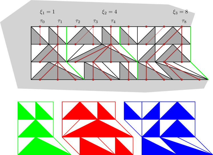
Figure 7: Block decomposition of the half-slice $\mathcal{H}\mathcal{L}_{-3}^{0}$. The first block is pictured in green, the second one in red, the third one in blue. In the upper figure, we represented the skeleton in brown (with trees of height $3$ in thick lines), slots in dark gray, and the left-most geodesics following the right boundary of trees of height $3$ in green. In this example, $\xi_{1}=1$, $\xi_{2}=4$, $\xi_{3}=8$.

The skeleton of $\mathcal{L}$ is made of i.i.d. trees, thus all the blocks $\mathcal{H}\mathcal{L}_{j^{\prime}}^{j}(n)$, viewed as planar maps with a boundary, are independent and share the same law, which only depends on $j-j^{\prime}$.

The thickness of the $n$-th block $\operatorname{Thickness}(\mathcal{H}\mathcal{L}_{j^{\prime}}^{j}(n))$ (called diameter in [4]) is the minimal graph distance in this block between a point of its left boundary and a point of its right boundary. Note that the thickness of a block cannot be $0$, since the presence of a tree of maximal height implies that the left-most geodesics corresponding to the left and right boundary of the block do not coalesce (by a previous remark).

Furthermore, the thickness of $\mathcal{H}\mathcal{L}_{j^{\prime}}^{j}(n)$ is always smaller than $j-j^{\prime}+1$. Indeed, the left-most geodesic started at $(\xi_{n-1}+1,j)$ (i.e. the left boundary) and the left-most geodesic started at $(\xi_{n},j)$ coalesce before height $j^{\prime}$ (i.e. after at most $j-j^{\prime}$ steps), since no tree rooted between $\xi_{n-1}+1$ and $\xi_{n}$ reaches height $j-j^{\prime}$. In this way, we get a path of length at most $j-j^{\prime}$ that connects the left boundary of the block to the vertex $(\xi_{n},j)$, and we just have to add the edge $((\xi_{n},j),(\xi_{n}+1,j))$ to get the desired bound.

It will be useful to note the following simple fact: any path that stays in the half-slice $\mathcal{H}\mathcal{L}_{j^{\prime}}^{j}$ with one endpoint on the left side of the left boundary of some $\mathcal{H}\mathcal{L}_{j^{\prime}}^{j}(n)$, and its other endpoint on the right side of its right boundary, has a length which is at least the thickness of the block.

Let us outline the key idea of the proof of Proposition 8. A path of length $r$ between two vertices of the boundary of $\mathcal{L}$ cannot exit the slice $\mathcal{L}_{-h}^{0}$ for any $h\geq r$. We apply this observation with $h=\lceil Cr\rceil$ with some constant $C\geq 1$. If we fix $K>0$ large enough, then with high probability we will find a block of $\mathcal{L}_{-h}^{0}$ with top boundary included in $[A,A+Kr^{2}]\times\{0\}$, and any path in $\mathcal{L}_{-h}^{0}$ that goes from the left side to the right side of $[A,A+Kr^{2}]\times\{0\}$ must cross this block. All we need to conclude is the fact that we can choose $h$ such this block has thickness at least $r$ with high probability.

The latter fact is derived from the following result, which is adapted from [4, theorem 5]. For every integer $h>0$, let $\mathcal{G}(h)$ be a random variable with the law of a block of height $h$. Fix $\varepsilon\in(0,1)$. The $\varepsilon$-quantile $f_{\varepsilon}(h)$ of the thickness of $\mathcal{G}(h)$ is the largest integer $n$ such that

$$\mathbb{P}(\operatorname{Thickness}(\mathcal{G}(h))\geq n)\geq 1-\varepsilon.$$ (9)

Note that $1\leq f_{\varepsilon}(h)\leq h+1$ by previous observations.

Proposition 9.

For every $\varepsilon\in(0,1)$, there exists $C_{\varepsilon}\in(0,1)$ such that for every $h\geq 1$, $f_{\varepsilon}(h)\geq C_{\varepsilon}h$.

We postpone the proof of Proposition 9 to the next section and complete the proof of Proposition 8.

Proof of Proposition 8.

Let $r\geq 1$, and set $h={\left\lceil r/C_{\varepsilon/4}\right\rceil}$, where $C_{\varepsilon/4}$ is given by Proposition 9, and consider the first block of the half-slice $\mathcal{L}_{-h}^{0}$, that is, $\mathcal{H}\mathcal{L}_{-h}^{0}(1)$ with the previous notation. By Proposition 9, we have

$$\mathbb{P}(\operatorname{Thickness}(\mathcal{H}\mathcal{L}_{-h}^{0}(1))\geq r) \geq\mathbb{P}(\operatorname{Thickness}(\mathcal{H}\mathcal{L}_{-h}^{0}(1))\geq C_{\varepsilon/4}h)$$

$$\geq\mathbb{P}(\operatorname{Thickness}(\mathcal{H}\mathcal{L}_{-h}^{0}(1))\geq f_{\varepsilon/4}(h))$$

$$\geq 1-\varepsilon/4.$$

Let $\mathcal{E}_{1}$ denote the event $\{\operatorname{Thickness}(\mathcal{H}\mathcal{L}_{-h}^{0}(1))\geq r\}$.

The right-most point of the top boundary of $\mathcal{H}\mathcal{L}_{-h}^{0}(1)$ is $(\xi_{1}+1,0)$, where $\xi_{1}$ follows a geometric law with parameter $1-\pi_{h}\geq c/r^{2}$ for some constant $c>0$ independent of $r$ (cf. Proposition 4). We can take $K>0$ large enough so that $\xi_{1}+1\leq Kr^{2}$ holds with probability larger than $1-\varepsilon/4$. Let us call $\mathcal{E}_{2}$ the event where $\xi_{1}+1\leq Kr^{2}$.

On the event $\mathcal{E}_{1}\cap\mathcal{E}_{2}$ of probability at least $1-\varepsilon/2$ the block $\mathcal{H}\mathcal{L}_{-h}^{0}(1)$ has thickness at least $r$ and its top boundary is contained in $[0,Kr^{2}]\times\{0\}$. Then any two points $(i,0)$ and $(i^{\prime},0)$ with $i\leq 0$ and $i^{\prime}\geq Kr^{2}$ are at $\mathrm{d}_{\mathrm{gr}}^{\mathcal{L}}$-distance at least $r$, since any path of length smaller than $r$ linking them necessarily crosses the block $\mathcal{H}\mathcal{L}_{-h}^{0}(1)$.

From an obvious argument of translation invariance, we obtain that for any integer $A>0$, with probability larger than $1-\varepsilon/2$, any point in $(\-\infty,A]\times\{0\}$ and any point in $[A+Kr^{2},+\infty)\times\{0\}$ are at $\mathrm{d}_{\mathrm{gr}}^{\mathcal{L}}$-distance at least $r$. Similarly, with probability larger than $1-\varepsilon/2$ the two half-lines $(\-\infty,-A-Kr^{2}]\times\{0\}$ and $[-A,+\infty)\times\{0\}$ are also at $\mathrm{d}_{\mathrm{gr}}^{\mathcal{L}}$-distance larger than $r$. The statement of the proposition follows. ∎

3.3.2 Proof of Proposition 9

For $h\geq 6$ and $m\in\{1,2,\ldots,{\left\lfloor\frac{h}{6}\right\rfloor}\}$, we set

$$J_{m}=\left\{0,-m,-2m,...,-\left({\left\lfloor\frac{h}{m}\right\rfloor}-3\right)m,-h+3m\right\}.$$

We write $\mathcal{G}(h)$ for a block of height $h$, and $\mathcal{G}_{j^{\prime}}^{j}(h)$ for the slice of $\mathcal{G}(h)$ contained between heights $j^{\prime}$ and $j$, for $-h\leq j^{\prime}<j\leq 0$. We recall that $\varepsilon\in(0,1)$ is fixed.

Lemma 10.

There exists $C\in(0,1/6)$ s.t. for all $h$ large enough and $0<m\leq Ch$, the following property holds with probability at least $1-\varepsilon$: for every $j\in J_{m}$, the length of any path connecting the left boundary of $\mathcal{G}(h)$ to its right boundary and staying in $\mathcal{G}_{j-3m}^{j}(h)$ is at least $C{\left(\frac{h}{m}\right)}^{2}f_{\varepsilon}(m)$.

As a technical ingredient of the proof of Lemma 10, we need a uniform lower bound on the size of the block at every generation. For $0\leq k\leq h$, let $X_{k}(h)$ denote the number of vertices of the skeleton of $\mathcal{G}(h)$ at generation $k$.

Lemma 11.

There exists a constant $C_{1}>0$ which does not depend of $h$, such that

$$\mathbb{P}\left(\inf_{0\leq k\leq h}X_{k}(h)>C_{1}h^{2}\right)\geq 1-\varepsilon/2.$$ (10)

See [4, Lemma 2] for a proof of Lemma 11.

Proof of Lemma 10.

The idea is to choose $C^{\prime}$ small enough so that with high probability, one can find at least $C^{\prime}(h/m)^{2}$ blocks of thickness at least $f_{\varepsilon}(m)$ inside the slice $\mathcal{G}_{j-3m}^{j}(h)$, for every $j\in J_{m}$. Any path connecting the left and right boundaries of this slice will then have length at least $C^{\prime}(h/m)^{2}f_{\varepsilon}(m)$.

We argue in the half-slice $\mathcal{H}\mathcal{L}_{-h}^{0}$. Note that the first block of this half-slice has the same law as $\mathcal{G}(h)$.

Let $C_{1}$ be chosen as in Lemma 11 so that (10) holds. Consider the half-slice $\mathcal{H}\mathcal{L}_{j-3m}^{j}$ for $j\in J_{m}$, and let $k$ be a positive integer. The number of blocks of this slice whose top boundary lies in $[0,{\left\lceil C_{1}h^{2}\right\rceil}]\times\{j\}$ is distributed as the number of trees with height at least $3m$ in a forest of ${\left\lceil C_{1}h^{2}\right\rceil}$ independent Bienaymé-Galton-Watson trees with offspring distribution $\theta$. Each block has a probability greater than $1-\varepsilon$ of having thickness at least $f_{\varepsilon}(3m)$. The number $N_{j}$ of blocks with thickness at least $f_{\varepsilon}(3m)$ and top boundary in $[0,{\left\lceil C_{1}h^{2}\right\rceil}]\times\{j\}$ is then bounded below in distribution by a binomial variable with parameters $({\left\lceil C_{1}h^{2}\right\rceil},(1-\varepsilon)(1-\pi_{3m}))$, where $\pi_{s}$ is defined in Proposition 4. By standard large deviation estimates for the binomial distribution and the bound $1-\pi_{s}\geq c/s^{2}$, we can find $C,C^{\prime},C^{\prime\prime}>0$ such that for all large enough $h$, for every $m\leq Ch$, for every $j\in J_{m}$

$$\mathbb{P}\left(N_{j}<C^{\prime}{\left(\frac{h}{m}\right)}^{2}\right)<\exp\left(-C^{\prime\prime}{\left(\frac{h}{m}\right)}^{2}\right).$$

Summing over $j\in J_{m}$ and taking $C$ even smaller if necessary, we get

$$\mathbb{P}\left(\forall j\in J_{m}\ :\ N_{j}\geq C{\left(\frac{h}{m}\right)}^{2}\right)\geq 1-\varepsilon/2.$$ (11)

On the event of probability at least $1-\varepsilon/2$ considered in Lemma 11, the first ${\left\lceil C_{1}r^{2}\right\rceil}$ vertices of the skeleton of $\mathcal{H}\mathcal{L}_{-r}^{0}$ at generation $j$ (i.e. the first ${\left\lceil C_{1}r^{2}\right\rceil}$ vertices of the skeleton of $\mathcal{H}\mathcal{L}_{j-3m}^{j}$) belong to the first block $\mathcal{H}\mathcal{L}_{-r}^{0}(1)$, thus the $N_{j}$ blocks of thickness at least $f_{\varepsilon}(3m)$ considered above are contained in $\mathcal{H}\mathcal{L}_{-r}^{0}(1)$. The property of Lemma 10 then holds on the intersection of the event in Lemma 11 with the event in (11). ∎

Proposition 9 will be proved via the following functional inequality on $f_{\varepsilon}$:

Proposition 12.

Let $C\in(0,1/6)$ be as in Lemma 10. Then for all $h$ large enough,

$$f_{\varepsilon}(h)\geq C\max_{1\leq m\leq Ch}\min\left(m,{\left(\frac{h}{m}\right)}^{2}f_{\varepsilon}(3m)\right).$$ (12)

Proof.

The idea is to cut the block into slices of height $3m$, and to consider separately the cases where the shortest path crossing the block from left to right stays inside such a slice or not. See Figure 8 for an illustration.

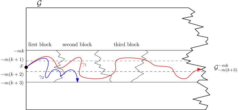
Figure 8: Paths started from a point $x$ on the left boundary can either stay in a slice of height $3m$ around $x$ (and have length at least $C{\left(\frac{h}{m}\right)}^{2}f_{\varepsilon}(m)$ by Lemma 10 w.h.p.), or leave it and have length at least $m$ a.s..

Let $m$ be an integer with $1\leq m\leq Ch$. Consider a path $\gamma$ in $\mathcal{G}(h)$ that achieves the thickness of this block, and let $x$ be its starting point on the left boundary. We assume for simplicity that $x$ is at distance at least $m$ from the top and bottom boundaries (the case where $x$ is at distance smaller than $m$ from the top or bottom boundaries is treated similarly). By our choice of $J_{m}$, there is always an index $j\in J_{m}$ such that $x$ is in the slice $\mathcal{G}_{j-2m}^{j-m}(h)$. Then either $\gamma$ leaves the slice $\mathcal{G}_{j-3m}^{j}(h)$, which takes at least $m$ steps; or $\gamma$ stays in $\mathcal{G}_{j-3m}^{j}(h)$, but then by Lemma 10 its length is at least $C{\left(\frac{h}{m}\right)}^{2}f_{\varepsilon}(m)$ with probability at least $1-\varepsilon$.

We conclude that the thickness of $\mathcal{G}(h)$ is at least $C\min\left(m,{\left(\frac{h}{m}\right)}^{2}f_{\varepsilon}(m)\right)$ with probability at least $1-\varepsilon$. Hence $f_{\varepsilon}(m)\geq C\min\left(m,{\left(\frac{h}{m}\right)}^{2}f_{\varepsilon}(m)\right)$. Since this holds for all $m$ with $1\leq m\leq Ch$, this gives the result of Proposition 12. ∎

Proof of Proposition 9.

First note that by taking $C$ smaller if necessary we may assume that the bound of Proposition 12 holds for every $h\geq{\left\lfloor 6/C^{2}\right\rfloor}$. We then prove by induction that $f_{\varepsilon}(h)\geq\frac{C^{2}}{6}h$ for every $h\geq 1$. If $h\leq{\left\lfloor 6/C^{2}\right\rfloor}$ this bound is trivial. So let $h_{0}\geq{\left\lfloor 6/C^{2}\right\rfloor}$ and assume that $f_{\varepsilon}(h)\geq\frac{C^{2}}{6}h$ for every $1\leq h\leq h_{0}$. Take $h=h_{0}+1$ and $m={\left\lfloor Ch/3\right\rfloor}$. One verifies that $3m\leq Ch<h$, hence $3m\leq h_{0}$, so by our assumption $f_{\varepsilon}(3m)\geq C^{2}m/2$.

We note as well that $\frac{Ch}{3}>\frac{C}{3}\frac{6}{C^{2}}=\frac{2}{C}>12$, so that ${\left\lfloor\frac{Ch}{3}\right\rfloor}\geq\frac{Ch}{6}$, hence $m\geq Ch/6$.

By Proposition 12,

$$f_{\varepsilon}(h)\geq C\min\left(m,{\left(\frac{h}{m}\right)}^{2}f_{\varepsilon}(3m)\right)\geq C\min\left(\frac{Ch}{6},{\left(\frac{3}{C}\right)}^{2}\frac{C^{2}}{2}\frac{Ch}{6}\right)$$

This completes the proof. ∎

3.4 Subadditivity

It will be convenient to consider the map $\widetilde{\mathcal{L}}$ which is derived from the lhpq $\mathcal{L}$ be removing all “horizontal edges” $((j,0),(j+1,0))$ for $j\in\mathbb{Z}$. For every integer $j<0$, we also denote by $\widetilde{\mathcal{L}}_{-\infty}^{j}$ the submap of $\widetilde{\mathcal{L}}$ (or of $\mathcal{L}$) contained in the half-plane below ordinate $j$. If $-\infty<j<j^{\prime}\leq 0$, $\widetilde{\mathcal{L}}_{j}^{j^{\prime}}$ is the submap of $\widetilde{\mathcal{L}}$ contained in $\mathbb{R}\times[j,j^{\prime}]$. We equip the vertex sets of these graphs with the first-passage percolation distance induced by i.i.d. weights to the edges (the common distribution of these weights is supported on $[1,\kappa]$). Recall our notation $\rho=(0,0)$ for the root vertex of $\mathcal{L}$ (or of $\widetilde{\mathcal{L}}$), and $\partial_{j}\mathcal{L}$ for the line at vertical coordinate $j\leq 0$ (viewed here as a collection of vertices).

Proposition 13.

There exists a constant $\textbf{c}_{p}\in[1,\kappa]$ such that

$$r^{-1}\mathrm{d}_{\mathrm{fpp}}^{\widetilde{\mathcal{L}}}(\rho,\partial_{-r}\mathcal{L})\overset{\text{a.s.}}{\underset{r\to\infty}{\longrightarrow}}\textbf{c}_{p}.$$

Proof.

We derive this proposition from the subadditive ergodic theorem. Let $-\infty<j^{\prime}<j<0$, and let $x_{j}$ be the left-most vertex of $\partial_{j}\mathcal{L}$ such that $\mathrm{d}_{\mathrm{fpp}}^{\widetilde{\mathcal{L}}}(\rho,\partial_{j}\mathcal{L})=\mathrm{d}_{\mathrm{fpp}}^{\widetilde{\mathcal{L}}}(\rho,x_{j})$. Then,

$$\mathrm{d}_{\mathrm{fpp}}^{\widetilde{\mathcal{L}}_{j^{\prime}}^{0}}(\rho,\partial_{j^{\prime}}\mathcal{L})\leq\mathrm{d}_{\mathrm{fpp}}^{\widetilde{\mathcal{L}}_{j}^{0}}(\rho,\partial_{j}\mathcal{L})+\mathrm{d}_{\mathrm{fpp}}^{\widetilde{\mathcal{L}}_{j^{\prime}}^{j}}(x_{j},\partial_{j^{\prime}}\mathcal{L}).$$

Note that $x_{j}$ is a function of $\widetilde{\mathcal{L}}_{j}^{0}$ and of the weights on edges of $\widetilde{\mathcal{L}}_{j}^{0}$. Thanks to the independence of layers of the map, $\mathrm{d}_{\mathrm{fpp}}^{\widetilde{\mathcal{L}}_{j^{\prime}}^{j}}(x_{j},\partial_{j^{\prime}}\mathcal{L})$ is independent of $\mathrm{d}_{\mathrm{fpp}}^{\widetilde{\mathcal{L}}_{j}^{0}}(\rho,\partial_{j}\mathcal{L})$ and has the same distribution as $\mathrm{d}_{\mathrm{fpp}}^{\widetilde{\mathcal{L}}_{j^{\prime}-j}^{0}}(\rho,\partial_{j^{\prime}-j}\mathcal{L})$. We then apply Liggett’s version of Kingman’s subadditive ergodic theorem [16, theorem 1.10] to conclude that

$$r^{-1}\mathrm{d}_{\mathrm{fpp}}^{\widetilde{\mathcal{L}}_{-r}^{0}}(\rho,\partial_{-r}\mathcal{L})\overset{\text{a.s.}}{\underset{r\to\infty}{\longrightarrow}}\textbf{c}_{p}$$

for some constant $\textbf{c}_{p}$. The fact that $\textbf{c}_{p}\in[1,\kappa]$ is immediate since weights belong to $[1,\kappa]$ and the graph distance from $\rho$ to $\partial_{-r}\mathcal{L}$ (in $\widetilde{\mathcal{L}}_{-r}^{0}$) is equal to $r$. The lemma follows by noting that $\mathrm{d}_{\mathrm{fpp}}^{\widetilde{\mathcal{L}}}(\rho,\partial_{j}\mathcal{L})=\mathrm{d}_{\mathrm{fpp}}^{\widetilde{\mathcal{L}}_{j}^{0}}(\rho,\partial_{j}\mathcal{L})$.

∎

4 Technical tools

4.1 Density between the LHPQ and truncated hulls of the UIPQ

Proposition 7 suggests that the neighborhood of a vertex chosen uniformly on the boundary of a large hull in the uipq looks like the lhpq. We will need a quantitative version of this property; this is provided by Proposition 14, whose proof does not depend on Proposition 7.

Let $a\in(0,1)$, let $(\tau_{i})_{i\in\mathbb{Z}}$ be an i.i.d. Bienaymé-Galton-Watson forest with offspring distribution $\theta$, and for every integer $r\geq 1$, let $N_{r}^{(a)}$ be a random variable distributed uniformly over $\{{\left\lfloor ar^{2}\right\rfloor}+1,...,{\left\lfloor r^{2}/a\right\rfloor}\}$, and independent of $(\tau_{i})_{i\in\mathbb{Z}}$. We denote the tree $\tau_{i}$ truncated at height $r$ by $[\tau_{i}]_{r}$ (we only keep vertices at generation at most $r$). For every $0\leq r<s$, let $\mathcal{F}_{r,s}$ be the forest defined from the skeleton of the annulus $\mathcal{C}(r,s)$ in the uipq as explained at the end of Section 2.

Proposition 14.

For every $a\in(0,1)$, we can find $C_{a}>0$ such that for every large enough integer $r$, for every choice of the integers $s>r$ and ${\left\lfloor ar^{2}\right\rfloor}+1\leq p,q\leq{\left\lfloor r^{2}/a\right\rfloor}$, for every forest $\mathcal{F}\in\mathbb{F}_{s-r,p,q}$,

$$\mathbb{P}\left(\mathcal{F}_{r,s}=\mathcal{F}\right)\leq C_{a}\mathbb{P}\left(([\tau_{1}]_{s-r},...,[\tau_{N^{(a)}_{r}}]_{s-r})=\mathcal{F}\right).$$ (13)

Proof.

By Proposition 5, for $\mathcal{F}\in\mathbb{F}_{s-r,p,q}$,

$$\mathbb{P}(\mathcal{F}_{s,r}=\mathcal{F}\ |\ H_{r}=p)=\frac{p}{q}\frac{2^{q}\kappa_{q}}{2^{p}\kappa_{p}}\prod_{v\in\mathcal{F}^{*}}\theta(c_{v}).$$ (14)

where we recall that $\mathcal{F}^{*}$ is the set of vertices at generation at most $s-r-1$ in the forest $\mathcal{F}$.

Let us consider the right-hand side of (13). Using the asymptotics (3), we find $C>0$ that only depends on $a$ such that for every large enough $r$, for every ${\left\lfloor ar^{2}\right\rfloor}<p,q<{\left\lfloor r^{2}/a\right\rfloor}$, we have $\frac{p}{q}\frac{2^{q}\kappa_{q}}{2^{p}\kappa_{p}}\leq C$. On the other hand, Proposition 4 and (3) allow us to find $C^{\prime}>0$ such that $\mathbb{P}(H_{r}=p)\leq C^{\prime}/r^{2}$ for every $r\geq 1$ and $p\geq 1$. From (14), we now get

$$\mathbb{P}\left(\mathcal{F}_{r,s}=\mathcal{F}\right)\leq\frac{CC^{\prime}}{r^{2}}\prod_{v\in\mathcal{F}^{*}}\theta(c_{v}).$$ (15)

On the other hand,

$$\mathbb{P}\left(([\tau_{1}]_{s-r},...,[\tau_{N^{(a)}_{r}}]_{s-r})=\mathcal{F}\right)=\mathbb{P}(N^{(a)}_{r}=q)\mathbb{P}(([\tau_{1}]_{s-r},...,[\tau_{q}]_{s-r})=\mathcal{F})=\frac{1}{{\left\lfloor r^{2}/a\right\rfloor}-{\left\lfloor ar^{2}\right\rfloor}}\prod_{v\in\mathcal{F}^{*}}\theta(c_{v}).$$ (16)

The desired result follows by comparing (15) and (16). ∎

4.2 Coalescence of left-most geodesics in the UIPQ

Left-most geodesics in the uipq coalesce quickly, in the following sense. Consider the set of all left-most geodesics started from the boundary of the hull of radius $r\geq 1$, and let $\gamma\in(0,1)$. Then the number of vertices at distance ${\left\lfloor\gamma r\right\rfloor}$ from the root that belong to one of these geodesics is bounded in distribution when $r$ is large. The next proposition (which is inspired from [6, Proposition 17]) gives a precise version of this property, which will be particularly useful in the proof of Proposition 16 below.

Recall that $\mathcal{H}^{\text{tr}}_{Q_{\infty}}(r)$ is the truncated hull of radius $r$ of the uipq ${Q_{\infty}}$ and that $\partial_{r}Q_{\infty}$ is the external boundary of this hull, which has length $H_{r}$. Pick a vertex $u_{0}^{(r)}$ on $\partial_{r}Q_{\infty}$ uniformly at random, and write $u^{(r)}_{0},u^{(r)}_{1},...u^{(r)}_{H_{r}-1}$ for all vertices of the boundary listed in clockwise order starting from $u_{0}^{(r)}$. We extend the definition of $u^{(r)}_{j}$ to all $j\in\mathbb{Z}$ by periodicity, so that $u^{(r)}_{j}=u^{(r)}_{j+H_{r}}$ for every $j$.

Proposition 15.

Let $\gamma\in(0,1/2)$ and $\delta>0$. For every integer $A>0$, let $\mathcal{X}_{r,A}$ be the event where any left-most geodesic to the root starting from a vertex of $\partial_{r}Q_{\infty}$ coalesces before time ${\left\lfloor\gamma r\right\rfloor}$ with one of the left-most geodesics started from $u^{(r)}_{{\left\lfloor kr^{2}/A\right\rfloor}}$, $0\leq k\leq{\left\lfloor\frac{AH_{r}}{r^{2}}\right\rfloor}$. Then we can choose $A$ large enough such that, for every sufficiently large $r$,

$$\mathbb{P}(\mathcal{X}_{r,A})\geq 1-\delta.$$

Proof.

The vertices $u^{(r)}_{{\left\lfloor kr^{2}/A\right\rfloor}}$, $0\leq k\leq{\left\lfloor\frac{AH_{r}}{r^{2}}\right\rfloor}$ divide $\partial_{r}Q_{\infty}$ into a collection of “intervals” made of consecutive edges of the boundary. We call an interval bad if at least two trees of the skeleton of $\mathcal{H}^{\text{tr}}_{Q_{\infty}}(r)$ rooted in this interval have height at least ${\left\lfloor\gamma r\right\rfloor}$ and good otherwise.

Now recall the observations made in Section 2 before discussing the law of the skeleton of the uipq. It follows that, if an interval $S$ is good, then the left-most geodesic started from any vertex of $S$ coalesces with one of the two left-most geodesics started from the endpoints of $S$. The proposition then reduces to proving that we can choose $A>0$ such that, for all $r$ large enough, the probability of having no bad interval is greater than $1-\delta$.

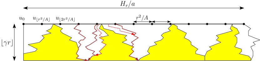
Figure 9: As soon as there are no bad intervals, every left-most geodesic started at a vertex $v$ of the top boundary coalesces before time $\gamma r$ with the left-most geodesic started at one of the endpoints of the interval that contains $v$. By choosing $A$ large enough, we ensure that with high probability there is no bad interval.

From the explicit law of the perimeter of truncated hulls in Proposition 4, we get that there exists $a\in(0,1)$ such that for all large enough $r$,

$$\mathbb{P}\left(H_{r}\notin\left[{\left\lfloor ar^{2}\right\rfloor}+1,{\left\lfloor r^{2}/a\right\rfloor}\right]\hbox{ or }H_{{\left\lfloor\gamma r\right\rfloor}}\notin\left[{\left\lfloor ar^{2}\right\rfloor}+1,{\left\lfloor r^{2}/a\right\rfloor}\right]\right)<\delta/2.$$ (17)

Consider first a forest made of ${\left\lfloor r^{2}/A\right\rfloor}+1$ independent Bienaymé-Galton-Watson trees with offspring distribution $\theta$. Simple estimates show that the probability that at least two trees of the forest have height greater than or equal to ${\left\lfloor\gamma r\right\rfloor}$ is bounded by $C(A\gamma)^{-2}$ (use Proposition 4) independently of $r$. If we now consider ${\left\lfloor A/a\right\rfloor}+1$ independent such forests, the probability that at least one of these forests satisfies the preceding property is bounded above by $C\left({\left\lfloor A/a\right\rfloor}+1\right)(A\gamma)^{-2}$, with a constant $C$ that does not depend on $r$ nor on $A$. By choosing $A$ large, the latter quantity can be made smaller than $\delta/(2C_{a})$, where $C_{a}$ is the constant in Proposition 14. The proof is completed by using Proposition 14 and (17). ∎

5 Main results for the first-passage percolation distance on quadrangulations

5.1 Distance through a thin annulus

Recall the constant $\textbf{c}_{p}$ introduced in Proposition 13.

Proposition 16.

Let $\varepsilon\in(0,1)$ and $\delta>0$. For every $\eta>0$ small enough, for all sufficiently large $n$, the property

$$(1-\varepsilon)\textbf{c}_{p}\eta n\leq\mathrm{d}_{\mathrm{fpp}}^{Q_{\infty}}(v,\partial_{n-{\left\lfloor\eta n\right\rfloor}}Q_{\infty})\leq(1+\varepsilon)\textbf{c}_{p}\eta n$$ (18)

holds for every $v\in\partial_{n}Q_{\infty}$, with probability at least $1-\delta$.

The proof of this result is technical but very similar to the proof of [6, Proposition 19], to which we refer for additional details. Let us start by an outline of the main ideas of the proof. Recalling the absolute continuity relations stated in Proposition 14, we observe that a sufficiently thin slice of the uipq (of the form $\mathcal{C}(n-{\left\lfloor\eta n\right\rfloor},n)$), seen from a uniformly chosen vertex of its outer boundary, looks like a slice of the lhpq. This in turn allows us to use Proposition 13.

In order to implement the latter observation, we need to make sure that with high probability, distances from a point $v$ of the top boundary of the annulus $\mathcal{C}(n-{\left\lfloor\eta n\right\rfloor},n)$ to the bottom boundary are determined by a “small” neighborhood of $v$ in the annulus. This essentially follows from the control of distances along the boundary discussed in Section 3.3.

Finally, we need (18) to hold simultaneously for all $v$ on the top boundary. Proposition 15 ensures that with high probability, the left-most geodesic started at a vertex $v$ of the top boundary coalesces quickly with one of the left-most geodesics started from a bounded number of points on the top boundary. Thanks to this observation, it is enough to verify that (18) holds for a bounded number of vertices $v\in\partial_{n}Q_{\infty}$.

Proof of Proposition 16.

In a way similar to Section 3.4, we let $\widetilde{\mathcal{H}}_{Q_{\infty}}(n)$ denote the map obtained from $\mathcal{H}^{\text{tr}}_{Q_{\infty}}(n)$ by removing the edges of the external boundary. It is then convenient to write $\mathrm{d}_{\mathrm{gr}}^{(n)}$ for the graph distance on $\widetilde{\mathcal{H}}_{Q_{\infty}}(n)$, and similarly $\mathrm{d}_{\mathrm{fpp}}^{(n)}$ for the first-passage percolation distance on $\widetilde{\mathcal{H}}_{Q_{\infty}}(n)$ (in both cases we allow only paths made of edges of $\widetilde{\mathcal{H}}_{Q_{\infty}}(n)$). Similarly as in the proof of Proposition 15, we pick a vertex $u^{(n)}_{0}$ uniformly at random on $\partial_{n}Q_{\infty}$, and denote the vertices of $\partial_{n}Q_{\infty}$ in clockwise order starting from $u^{(n)}_{0}$ by $(u^{(n)}_{j})_{0\leq j<H_{n}}$. We extend the definition of $u^{(n)}_{j}$ to $j\in\mathbb{Z}$ by periodicity. Let $\delta\in(0,1)$.

First, we use Proposition 4 to fix $a\in(0,1)$ small enough such that, for every $\eta\in(0,1/2)$, the top and bottom perimeters of the annulus $\mathcal{C}(n-{\left\lfloor\eta n\right\rfloor},n)$ are both within the range $[an^{2},a^{-1}n^{2}]$ with probability at least $1-\delta/4$. In the remaining part of the proof, we implicitly argue on the event $\mathcal{E}_{\eta}^{(n)}$ where the latter properties hold. We also set $N=\lceil 9a^{-2}\rceil$.

Proposition 14 allows us to bound the probability of any event concerning the forest encoding the skeleton of $\mathcal{C}(n-{\left\lfloor\eta n\right\rfloor},n)$ by a constant times the probability of the same event concerning an i.i.d. forest of Bienaymé-Galton-Watson trees with offspring distribution $\theta$. In particular, by taking $\eta$ small enough, one can ensure that the left-most geodesics started at $u^{(n)}_{-{\left\lfloor an^{2}/4\right\rfloor}}$ and $u^{(n)}_{{\left\lfloor an^{2}/4\right\rfloor}}$ do not coalesce before reaching $\partial_{n-{\left\lfloor\eta n\right\rfloor}}Q_{\infty}$ except on a set of probability at most $\delta/(8N)$. On this event, the complement in the annulus $\mathcal{C}(n-{\left\lfloor\eta n\right\rfloor},n)$ of the union of the left-most geodesics started at $u^{(n)}_{-{\left\lfloor an^{2}/4\right\rfloor}}$ and at $u^{(n)}_{{\left\lfloor an^{2}/4\right\rfloor}}$ has two components, and we call $\mathcal{G}^{(n)}_{0}$ the one containing the part of $\partial_{n}Q_{\infty}$ between $u^{(n)}_{-{\left\lfloor an^{2}/4\right\rfloor}}$ and $u^{(n)}_{{\left\lfloor an^{2}/4\right\rfloor}}$ in clockwise order. The lateral boundary $\partial^{l}\mathcal{G}^{(n)}_{0}$ consists of the two left-most geodesics bounding $\mathcal{G}^{(n)}_{0}$, and the bottom boundary $\partial^{b}\mathcal{G}^{(n)}_{0}$ is defined in an obvious way.

Let us argue on the event where $\mathcal{G}^{(n)}_{0}$ is well-defined. Using Proposition 8 and Proposition 14, and taking $\eta$ even smaller if necessary, we can ensure that the following holds except on a set of probability at most $\delta/(8N)$: any point $u^{(n)}_{k}$ with $|k|\leq an^{2}/16$ is at $\mathrm{d}_{\mathrm{gr}}^{(n)}$-distance at least $(4\kappa+1)\eta n$ from $u^{(n)}_{-{\left\lfloor an^{2}/4\right\rfloor}}$ and $u^{(n)}_{{\left\lfloor an^{2}/4\right\rfloor}}$. By the triangle inequality, we thus obtain that on this event, the $\mathrm{d}_{\mathrm{gr}}^{(n)}$-distance between any point $u^{(n)}_{k}$ with $|k|\leq an^{2}/16$ and $\partial^{l}\mathcal{G}^{(n)}_{0}$ is at least $4\kappa\eta n$. Any path in the annulus $\mathcal{C}(n-{\left\lfloor\eta n\right\rfloor},n)$ with one endpoint in $\{u^{(n)}_{k},|k|\leq an^{2}/16\}$ and the other one in $\partial_{n-{\left\lfloor\eta n\right\rfloor}}Q_{\infty}$ that crosses $\partial^{l}\mathcal{G}^{(n)}_{0}$ will have length at least $4\eta\kappa n$, and thus first-passage percolation weight at least $4\eta\kappa n$. On the other hand, the left-most geodesic started at any $u^{(n)}_{k},|k|\leq an^{2}/16$, gives a path of length at most $\eta n$ between $u^{(n)}_{k}$ and $\partial_{n-{\left\lfloor\eta n\right\rfloor}}Q_{\infty}$, that is thus of first-passage-percolation weight at most $\kappa\eta n$. It follows that no $\mathrm{d}_{\mathrm{fpp}}^{(n)}$-shortest path between a vertex of the form $u^{(n)}_{k}$, $|k|\leq an^{2}/16$, and $\partial_{n-{\left\lfloor\eta n\right\rfloor}}Q_{\infty}$ reaches $\partial^{l}\mathcal{G}^{(n)}_{0}$, except on an event of probability at most $\delta/(8N)$.

The previous considerations apply as well if we replace $u^{(n)}_{0}$ by $u^{(n)}_{j}$ for any $j$ (possibly depending on $n$). Let $\mathcal{G}^{(n)}_{j}$ stand for the analog of $\mathcal{G}^{(n)}_{0}$ when $u^{(n)}_{0}$ is replaced by $u^{(n)}_{j}$. We obtain that, except possibly on an event of probability at most $\delta/4$, for every $j$ of the form $j=i{\left\lfloor an^{2}/8\right\rfloor}$, $0\leq i\leq N-1$, the set $\mathcal{G}^{(n)}_{j}$ is well-defined and for every integer $k$ with $j-{\left\lfloor an^{2}/16\right\rfloor}\leq k\leq j+{\left\lfloor an^{2}/16\right\rfloor}$, any $\mathrm{d}_{\mathrm{fpp}}^{(n)}$-shortest path from $u^{(n)}_{k}$ to $\partial_{n-{\left\lfloor\eta n\right\rfloor}}Q_{\infty}$ reaches the bottom boundary of $\mathcal{G}^{(n)}_{j}$ before its lateral boundary. We write $\mathcal{D}^{(n)}_{\eta}$ for the event of probability at least $1-\delta/4$ where the preceding properties hold. On the intersection $\mathcal{E}^{(n)}_{\eta}\cap\mathcal{D}^{(n)}_{\eta}$, for any choice of $j$ and $k$ as previously, the $\mathrm{d}_{\mathrm{fpp}}^{(n)}$-distance from $u^{(n)}_{k}$ to $\partial_{n-{\left\lfloor\eta n\right\rfloor}}Q_{\infty}$ can be computed from the information given by $\mathcal{G}^{(n)}_{j}$ and the weights on edges of $\mathcal{G}^{(n)}_{j}$. From our choice of $N$, we also see that the vertices $u^{(n)}_{k}$ with $j-{\left\lfloor an^{2}/16\right\rfloor}\leq k\leq j+{\left\lfloor an^{2}/16\right\rfloor}$ and $j$ of the form $j=i{\left\lfloor an^{2}/8\right\rfloor}$, $0\leq i\leq N-1$, cover the whole boundary $\partial_{n}Q_{\infty}$ (provided $\mathcal{E}^{(n)}_{\eta}$ holds).

At this stage, we use the absolute continuity relations in Proposition 14 in connection with Proposition 13. Let $j$ and $k$ be as previously (possibly depending on $n$). On the event $\mathcal{E}^{(n)}_{\eta}\cap\mathcal{D}^{(n)}_{\eta}$, the $\mathrm{d}_{\mathrm{fpp}}^{(n)}$-distance from $u^{(n)}_{k}$ to $\partial_{n-{\left\lfloor\eta n\right\rfloor}}Q_{\infty}$ is determined as a function of the skeleton of $\mathcal{G}^{(n)}_{j}$ (meaning the forest consisting of the trees of the skeleton of $\mathcal{C}(n-{\left\lfloor\eta n\right\rfloor},n)$ rooted at edges between $u^{(n)}_{j-{\left\lfloor an^{2}/4\right\rfloor}}$ and $u^{(n)}_{j+{\left\lfloor an^{2}/4\right\rfloor}}$ in clockwise order) and the quadrangulations that fill in the slots — and of course of the weights on edges. But the same function determines the first passage percolation distance in the lhpq (which is estimated by Proposition 13) and one just has to compare the distributions of skeletons, for which one may use Proposition 14. It follows that, on the event $\mathcal{E}^{(n)}_{\eta}\cap\mathcal{D}^{(n)}_{\eta}$, we have

$$\mathrm{d}_{\mathrm{fpp}}^{(n)}(u^{(n)}_{k},\partial_{n-{\left\lfloor\eta n\right\rfloor}}Q_{\infty})\ \in\ [(1-\varepsilon/2)\textbf{c}_{p}\eta n,(1+\varepsilon/2)\textbf{c}_{p}\eta n].$$ (19)

except possibly on an event of probability tending to $0$ as $n\to\infty$.

We now want to argue that (19) holds simultaneously for all $k$ outside a set of small probability. To this end, we rely on the coalescence of geodesics (Proposition 15). Let $A$ be chosen as in Proposition 15, replacing $\gamma$ by $\textbf{c}_{p}\eta\varepsilon/(4\kappa)$ and $\delta$ by $\delta/4$. As in Proposition 15, consider indices $k$ of the form ${\left\lfloor in^{2}/A\right\rfloor}$, $0\leq i\leq{\left\lfloor A/a\right\rfloor}$. Then, for $n$ large enough, (19) holds simultaneously for all these values of $k$, on the event $\mathcal{E}^{(n)}_{\eta}\cap\mathcal{D}^{(n)}_{\eta}$, except possibly on event of probability less than $\delta/4$. Furthermore, thanks to Proposition 15, we know on the event $\mathcal{E}^{(n)}_{\eta}\cap\mathcal{D}^{(n)}_{\eta}$ that, outside an event of probability at most $\delta/4$, every vertex $v\in\partial_{n}Q_{\infty}$ is at $\mathrm{d}_{\mathrm{gr}}^{(n)}$-distance at most $\varepsilon\textbf{c}_{p}\eta n/(2\kappa)$ (thus at $\mathrm{d}_{\mathrm{fpp}}^{(n)}$-distance at most $\varepsilon\textbf{c}_{p}\eta n/2$) from one of these vertices $u^{(n)}_{k}$. We conclude that we have $\mathrm{d}_{\mathrm{fpp}}^{(n)}(v,\partial_{n-{\left\lfloor\eta n\right\rfloor}}Q_{\infty})\in[(1-\varepsilon)\textbf{c}_{p}\eta n,(1+\varepsilon)\textbf{c}_{p}\eta n]$ for every vertex $v$ of $\partial_{n}Q_{\infty}$, outside an event of probability at most $\delta$. This is the desired result, except that we need to replace $\mathrm{d}_{\mathrm{fpp}}^{(n)}$ by $\mathrm{d}_{\mathrm{fpp}}^{Q_{\infty}}$. This is however easy since on one hand $\mathrm{d}_{\mathrm{fpp}}^{Q_{\infty}}\leq\mathrm{d}_{\mathrm{fpp}}^{(n)}$ and on the other hand the minimal values of $\mathrm{d}_{\mathrm{fpp}}^{(n)}(v,\partial_{n-{\left\lfloor\eta n\right\rfloor}}Q_{\infty})$ and $\mathrm{d}_{\mathrm{fpp}}^{Q_{\infty}}(v,\partial_{n-{\left\lfloor\eta n\right\rfloor}}Q_{\infty})$ on $\partial_{n}Q_{\infty}$ are the same. This completes the proof. ∎

5.2 Distance from the boundary of a hull to its center

The next step is to show that the distance from the root vertex of the uipq ${Q_{\infty}}$ to an arbitrary vertex of the boundary of a hull is close to a constant times the radius. Recall that $\rho$ is the root vertex of $Q_{\infty}$.

Proposition 17.

For every $\varepsilon\in(0,1)$,

$$\mathbb{P}\left((\textbf{c}_{p}-\varepsilon)n\leq\mathrm{d}_{\mathrm{fpp}}^{Q_{\infty}}(\rho,v)\leq(\textbf{c}_{p}+\varepsilon)n,\ \text{ for every }v\text{ in }\partial_{n}Q_{\infty}\right)\underset{n\to\infty}{\longrightarrow}1.$$

Proof.

Fix $\varepsilon\in(0,1)$, and take $\delta=\varepsilon^{2}/(5\kappa|\ln(\varepsilon/(5\kappa))|)$. For every $0<m<n$, we say that the annulus $\mathcal{C}(m,n)$ is good if, for every $v\in\partial_{n}Q_{\infty}$,

$$(1-\varepsilon/2)\textbf{c}_{p}\eta n\leq\mathrm{d}_{\mathrm{fpp}}^{Q_{\infty}}(v,\partial_{m}Q_{\infty})\leq(1+\varepsilon/2)\textbf{c}_{p}\eta n,$$ (20)

and it is bad otherwise. Proposition 16 ensures that we can fix $\eta\in(0,1)$ small enough such that for all $n$ large enough, the annulus $\mathcal{C}(n-{\left\lfloor\eta n\right\rfloor},n)$ is good with probability at least $1-\delta$.

Let $n_{0}=n$, and define by induction $n_{k+1}=n_{k}-{\left\lfloor\eta n_{k}\right\rfloor}$ for every $k\geq 0$. Let $q={\left\lfloor\frac{\ln(\varepsilon/(5\kappa))}{\ln(1-\eta)}\right\rfloor}$. Note that $n_{q}\geq\frac{\varepsilon}{5\kappa}n$ and $n_{q}\leq\frac{\varepsilon}{4\kappa}n$ for $n$ large. Using Markov’s inequality we get that for $n$ large enough,

$$\mathbb{P}\left(\#\{k\in\{0,1,…,q-1\}\ :\ \mathcal{C}(n_{k+1},n_{k})\text{ is bad}\}\ >\ \frac{\varepsilon}{5\kappa|\ln(1-\eta)|}\right)\leq\frac{5\kappa|\ln(1-\eta)|}{\varepsilon}q\delta\leq\varepsilon$$

by our choice of $\delta$ and $q$. Let $\mathcal{D}^{\varepsilon}_{n}$ denote the event whose probability appears in the previous display. We will show that the property $(\textbf{c}_{p}-\varepsilon)n\leq\mathrm{d}_{\mathrm{fpp}}^{Q_{\infty}}(\rho,v)\leq(\textbf{c}_{p}+\varepsilon)n$ for every $v\in\partial_{n}Q_{\infty}$ holds on the complement of $\mathcal{D}^{\varepsilon}_{n}$. Since $\mathbb{P}(\mathcal{D}^{\varepsilon}_{n})\leq\varepsilon$ for $n$ large, this will complete the proof.

Suppose that $\mathcal{D}^{\varepsilon}_{n}$ does not hold. Then the fpp-distance between any vertex $v\in\partial_{n}Q_{\infty}$ and $\rho$ is larger than the cost one must pay to cross the good annuli, that is

$$\mathrm{d}_{\mathrm{fpp}}^{Q_{\infty}}(v,\rho) \geq\sum_{k=0}^{q-1}(1-\varepsilon/2)\textbf{c}_{p}(n_{k}-n_{k+1})-\sum_{k\ :\ \mathcal{C}(n_{k+1},n_{k})\text{ bad}}(1-\varepsilon/2)\textbf{c}_{p}(n_{k}-n_{k+1})$$

$$\geq(1-\varepsilon/2)\textbf{c}_{p}(n_{0}-n_{q})-\frac{\varepsilon}{5\kappa|\ln(1-\eta)|}\textbf{c}_{p}\max_{0\leq k<q}(n_{k}-n_{k+1})$$

$$\geq\textbf{c}_{p}n\left[1-\frac{\varepsilon}{2}-\frac{\varepsilon}{4}-\frac{\varepsilon}{4|\ln(1-\eta)|}\eta\right]$$

$$\geq\textbf{c}_{p}n\left(1-\varepsilon\right),$$

using the properties $\kappa\geq 1$ and $\eta/|\ln(1-\eta)|<1$ for $\eta\in(0,1)$. Conversely, we can build a path from $v$ to $\rho$ that crosses the good annuli in the $\mathrm{d}_{\mathrm{fpp}}$-shortest way, and the bad annuli or the hull $\mathcal{H}^{\text{tr}}_{Q_{\infty}}(n_{q})$ along left-most geodesics. Using the properties $\mathrm{d}_{\mathrm{gr}}\leq\mathrm{d}_{\mathrm{fpp}}\leq\kappa\mathrm{d}_{\mathrm{gr}}$ and $1\leq\textbf{c}_{p}\leq\kappa$, we can bound its fpp-weight by

$$\sum_{k=0}^{q-1}(1+\varepsilon/2)\textbf{c}_{p}(n_{k}-n_{k+1})+\kappa n_{q}+\sum_{k\ :\ \mathcal{C}(n_{k+1},n_{k})\text{ bad}}\kappa(n_{k}-n_{k+1})$$

$$\leq(1+\varepsilon/2)\textbf{c}_{p}(n_{0}-n_{q})+\kappa\frac{\varepsilon}{4\kappa}n+\frac{\varepsilon}{5\kappa|\ln(1-\eta)|}\kappa\max_{0\leq k<q}(n_{k}-n_{k+1})$$

$$\leq\textbf{c}_{p}n\left[1+\frac{\varepsilon}{2}+\frac{\varepsilon}{4}+\frac{\varepsilon}{4|\ln(1-\eta)|}\eta\right]$$

$$\leq\textbf{c}_{p}n\left(1+\varepsilon\right),$$

giving $\mathrm{d}_{\mathrm{fpp}}^{Q_{\infty}}(v,\rho)\leq\textbf{c}_{p}n\left(1+\varepsilon\right)$. This completes the proof. ∎

5.3 Distance between two uniform points in finite quadrangulations

In this section, we consider a uniformly distributed rooted and pointed quadrangulation with $n$ faces, which we denote by $Q^{\bullet}_{n}$. The associated (unpointed) rooted quadrangulation is simply denoted by $Q_{n}$. We will write $\rho_{n}$ for the root vertex of $Q_{n}$ (or of $Q^{\bullet}_{n}$) and $\partial_{n}$ for the distinguished vertex of $Q^{\bullet}_{n}$. This notation will be in force throughout the remaining part of this work. We note that, conditionally on the unpointed map $Q_{n}$, $\partial_{n}$ is uniformly distributed over $V(Q_{n})$.

Our next goal is to control the fpp-distance between $\rho_{n}$ and $\partial_{n}$.

Proposition 18.

For every $\varepsilon\in(0,1)$,

$$\mathbb{P}\left(|\mathrm{d}_{\mathrm{fpp}}^{Q_{n}}(\rho_{n},\partial_{n})-\textbf{c}_{p}\mathrm{d}_{\mathrm{gr}}^{Q_{n}}(\rho_{n},\partial_{n})|>\varepsilon n^{1/4}\right)\underset{n\to\infty}{\longrightarrow}0.$$

We postpone the proof of this result to Section 5.4, and first give some technical tools that are needed in this proof.

The idea is to transfer the results that we established in the uipq to the setting of finite quadrangulations. The core tool that we establish in this section compares the law of a neighborhood of the root in the uipq and in a finite quadrangulation. In this direction, Proposition 20 gives a result valid for neighborhoods of diameter smaller than a constant times the typical diameter of the quadrangulation. This is closely related to [5, Lemma 8 and Proposition 9], but we need sharper results.

Let us briefly introduce the objects we need. Our proofs in this section and the next one make use of the (now classical) Cori-Vauquelin-Schaeffer bijection [15, Section 5.4] between rooted and pointed quadrangulations with $n$ faces, and labeled rooted plane trees with $n$ edges. For more details, we refer to [5, Section 4].

The Cori-Vauquelin-Schaeffer correspondence.

Consider a rooted plane tree $\tau$, with root vertex $\sigma$, together with a labeling $Z=(Z_{x})_{x\in V(\tau)}$ of its vertices by integers such that $Z_{\sigma}=0$, and $|Z_{x}-Z_{y}|\leq 1$ if $x$ and $y$ are adjacent. We fix $\epsilon\in\{0,1\}$ and explain how to get a pointed and rooted quadrangulation $Q$ from $(\tau,Z,\epsilon)$. To this end, we suppose that $\tau$ is embedded in the plane as shown on Figure 10. Then, firstly, we add a vertex $\partial$, and extend the labeling to $\partial$ so that $Z_{\partial}=-1+\min_{x\in V(\tau)}Z_{x}$. The vertex set of the quadrangulation $Q$ is $V(\tau)\cup\{\partial\}$, and $\partial$ is its distinguished vertex. We also extend the labeling to corners of $\tau$, by declaring that the label of a corner is the label of the incident vertex of $\tau$. Secondly, we order the corners of $\tau$ in clockwise order around $\tau$, starting from the bottom corner of $\sigma$. For every $n>Z_{\partial}+1$, we draw an edge of $Q$ from each corner labeled $n$ to the first next corner labeled $n-1$; and for each corner of index $Z_{\partial}+1$, we draw an edge from this corner to $\partial$. This defines the edges of $Q$. Finally, we root $Q$ at the edge drawn from the bottom corner of $\sigma$ and use $\epsilon$ to determine its orientation: the root vertex is $\sigma$ iff $\epsilon=1$. The construction should be clear from Figure 10. We mention the following important property relating labels on $\tau$ to distances from $\partial$ in $Q$: For every vertex $v\in V(Q)$, $\mathrm{d}_{\mathrm{gr}}^{Q}(\partial,v)=Z_{v}-Z_{\partial}$.

Figure 10: The CVS correspondence applied to a finite labeled tree (in black). The thick red edge is the root edge of the quadrangulation, and its orientation is determined by $\epsilon$ (here $\epsilon=1$).

The CVS correspondence allows us to code uniform rooted and pointed quadrangulations by uniform rooted labeled plane trees. More precisely, let $T_{n}$ be a uniform rooted plane tree with $n$ edges. Given $T_{n}$, assign i.i.d. weights on its edges, with uniform law over $\{-1,0,+1\}$. For every $x\in V(T_{n})$, define the label $Z^{n}_{x}$ as the sum of the weights of edges along the geodesic from the root to $x$ in $T_{n}$. Pick $\epsilon\in\{0,1\}$ uniformly at random. The CVS correspondence applied to $(T_{n},Z^{n},\epsilon)$ then gives a uniform rooted and pointed quadrangulation with $n$ faces.

Pruned trees.

Let $\tau$ be a (finite) rooted plane tree. For every vertex $v$ of $\tau$ and for every $h>0$ such that $\mathrm{d}_{\mathrm{gr}}^{\tau}(\sigma,v)\geq{\left\lfloor h\right\rfloor}$, we denote the ancestor of $v$ at height ${\left\lfloor h\right\rfloor}$ in $\tau$ by $[v]_{h}$. We construct the pruned tree $\mathcal{P}((\tau,v),h)$ by removing all strict descendants of $[v]_{h}$ in $\tau$ (see [5, Fig. 5]) and we see $\mathcal{P}((\tau,v),h)$ as a rooted plane tree pointed at $[v]_{h}$.

Note that the vertex set of $\mathcal{P}((\tau,v),h)$ is a subset of all vertices of $\tau$. It follows that, if $\tau$ is labeled by $Z$, we can construct a labeling of $\mathcal{P}((\tau,v),h)$ by restricting $Z$ to $V(\mathcal{P}((\tau,v),h))$. We will do so implicitely, keeping the same notation for the labeling on $\tau$ and on the pruned tree.

The case where $\tau$ is infinite is similar. In that case, we always assume that the tree has one end: there is only one infinite injective path started at its root, called the spine. We use the notation $[\infty]_{h}$ for the unique vertex of the spine at distance $h$ from the root, and remove its strict descendants in $\tau$ to get the pruned tree $\mathcal{P}(\tau,h)$. Informally, $\infty$ plays the role of the distinguished vertex.

We now state the first result of this section. Let $(\tau,Z)$ be a finite rooted labeled plane tree with root vertex $\sigma$. Let $\epsilon\in\{0,1\}$, and let $Q$ be the rooted and pointed quadrangulation constructed from $(\tau,Z,\epsilon)$ via the CVS correspondence (we denote the root vertex of $Q$ by $\rho$). Let $\xi\in V(\tau)$, and let $h$ be an integer such that $0<h<\mathrm{d}_{\mathrm{gr}}^{\tau}(\sigma,\xi)$. Set

$$r=-\min_{0\leq i\leq h}Z_{[\xi]_{i}}\geq 0.$$

Proposition 19.

Assume that $r\geq 4$. Then $B^{\bullet}_{Q}(r-3)$ is a function of the pruned tree $\mathcal{P}((\tau,\xi),h)$, its labeling, and $\epsilon$.

Proof.

The idea is to prove that, if $Q^{\prime}$ is the quadrangulation obtained by applying the CVS correspondence to the pruned tree, then $B^{\bullet}_{Q}(r-3)=B^{\bullet}_{Q^{\prime}}(r-3)$ (considered as an equality between rooted quadrangulations with a boundary).

Let us state some useful observations. Without loss of generality, by taking $h$ smaller we can assume that $Z_{[\xi]_{h}}=\min_{0\leq i\leq h}Z_{[\xi]_{i}}=-r$. We note that $\mathrm{d}_{\mathrm{gr}}^{Q}(\sigma,\rho)=0$ or $1$ depending on $\epsilon$. If $v\in V(\tau)$,

$$\mathrm{d}_{\mathrm{gr}}^{Q}(\sigma,v)\geq|Z_{\sigma}-Z_{v}|=|Z_{v}|,$$

and by the triangle inequality $\mathrm{d}_{\mathrm{gr}}^{Q}(\rho,v)\geq|Z_{v}|-1$.

Our first step is to prove that vertices of $B^{\bullet}_{Q}(r-3)$ “belong” to the pruned tree, and that their labels are at least $-r+1$.

Let $v$ be a vertex of $\tau$ such that $Z_{v}\leq-r$. Starting from any corner of $v$, the construction of edges in the CVS correspondence yields a path starting from $v$ that visits vertices with strictly decreasing labels. This path ultimately connects $v$ to $\partial$ by visiting only vertices with labels less than $-r$, thus at distance at least $r-1$ from $\rho$ in $Q$. By construction, any vertex of $B^{\bullet}_{Q}(r-3)$ is such that any path from this vertex to $\partial$ visits a vertex $w$ with $\mathrm{d}_{\mathrm{gr}}^{Q}(\rho,w)\leq r-2$. It follows that $v$ does not belong to $B^{\bullet}_{Q}(r-3)$.

Let us now check that vertices in $V(\tau)\setminus V(\mathcal{P}((\tau,\xi),h))$ do not belong to $B^{\bullet}_{Q}(r-3)$ either. Let $v$ be such a vertex with $Z_{v}>-r$ (the case $Z_{v}\leq-r$ was already considered above). Then $[\xi]_{h}$ is an ancestor of $v$, and the cactus bound [15, Proposition 5.9 (ii)] shows that

$$\mathrm{d}_{\mathrm{gr}}^{Q}(\sigma,v)\geq Z_{\sigma}-Z_{[\xi]_{h}}=r,$$

and thus $\mathrm{d}_{\mathrm{gr}}^{Q}(\rho,v)\geq r-1$.

Let $c$ be any corner of $v$. Order the corners of $\tau$ in clockwise order starting at $c$, and let $c^{\prime\prime}$ be the first corner of $[\xi]_{h}$ that appears in this enumeration: every corner between $c$ and $c^{\prime\prime}$ is incident to a vertex of $V(\tau)\setminus V(\mathcal{P}((\tau,\xi),h))$. Since labels change by at most $1$ in this enumeration, there will be a corner $c^{\prime}$ with label $Z_{v}-1$ between $c$ and $c^{\prime\prime}$ (possibly $c^{\prime}=c^{\prime\prime}$). This ensures that the edge drawn from $c$ in the CVS correspondence ends at a vertex in $V(\tau)\setminus V(\mathcal{P}((\tau,\xi),h))$ with label $Z_{v}-1$, or possibly at $[\xi]_{h}$. Therefore, we can inductively construct a path from $v$ that stays in $V(\tau)\setminus V(\mathcal{P}((\tau,\xi),h))$ until it reaches a vertex $w$ of label $-r$, and we extend this path to a path from $v$ to $\partial$ as we did previously. Every vertex of this path is at distance at least $r-1$ from $\rho$, so it follows again that $v$ does not belong to $B^{\bullet}_{Q}(r-3)$.

Note that by the same reasoning, if $c$ is a corner of label at least $-r+1$ that belongs to the pruned tree, then the edge drawn from $c$ will reach a vertex of the pruned tree (possibly $[\xi]_{h}$), and thus will be present in $Q^{\prime}$ as well as in $Q$.

As our second and last step, we now verify that $B^{\bullet}_{Q}(r-3)=B^{\bullet}_{Q^{\prime}}(r-3)$. By the first step, any edge belonging to $B^{\bullet}_{Q}(r-3)$ is drawn from a corner $c$ of $\tau$ (not incident to $[\xi]_{h}$) with label at least $-r+1$ that “belongs” to the pruned tree, so it appears both in $Q$ and $Q^{\prime}$. It follows that we have both

$$\mathrm{d}_{\mathrm{gr}}^{Q^{\prime}}(\rho,v)\leq\mathrm{d}_{\mathrm{gr}}^{Q}(\rho,v)\qquad\text{ if }v\in B^{\bullet}_{Q}(r-3),$$

$$\mathrm{d}_{\mathrm{gr}}^{Q}(\rho,v)\leq\mathrm{d}_{\mathrm{gr}}^{Q^{\prime}}(\rho,v)\qquad\text{ if }v\in B^{\bullet}_{Q^{\prime}}(r-3).$$

Next, any edge of the boundary of $B^{\bullet}_{Q}(r-3)$ is incident to a face of $Q$ containing a vertex at $\mathrm{d}_{\mathrm{gr}}^{Q}$-distance (hence $\mathrm{d}_{\mathrm{gr}}^{Q^{\prime}}$-distance) less than or equal to $r-4$ from $\rho$. This face must then also be contained in $B^{\bullet}_{Q^{\prime}}(r-3)$. It easily follows that $B^{\bullet}_{Q}(r-3)\subset B^{\bullet}_{Q^{\prime}}(r-3)$, and the converse is also true by a symmetric argument. ∎

The CVS correspondence can be extended to infinite labeled trees. Precisely, we consider the set $\SS$ of all infinite rooted labeled trees with one end, such that the infimum of the labels on the spine is $-\infty$. With every $(\tau,Z)\in\SS$ and $\varepsilon\in\{0,1\}$, one can associate an infinite planar quadrangulation $Q$, which is defined via a direct extension of the rules of the CVS correspondence (see [7, Proposition 2.5]). Furthermore, the preceding proposition is immediately extended to that case, with the same proof: for every integer $h>0$, if $r:=-\min\{Z_{[\infty]_{j}}:0\leq j\leq h\}\geq 4$, the hull $B^{\bullet}_{Q}(r-3)$ only depends on the pruned tree $\mathcal{P}(\tau,h)$, its labeling, and $\epsilon$.

The following proposition is closely related to [5, Proposition 9], but deals with hulls instead of balls. Recall that $Q^{\bullet}_{n}$ is uniformly distributed over the set of rooted and pointed quadrangulations with $n$ faces.

Proposition 20.

For every $\varepsilon>0$, there exists $\chi>0$ such that for every sufficiently large $n$, we can construct $Q^{\bullet}_{n}$ and ${Q_{\infty}}$ on the same probability space in such a way that the equality

$$B^{\bullet}_{Q^{\bullet}_{n}}(\chi n^{1/4})=B^{\bullet}_{{Q_{\infty}}}(\chi n^{1/4})$$

holds with probability at least $1-\varepsilon$.

Proof.

The proof is is very similar to that of [5, Proposition 9], using our Proposition 19 instead of [5, Proposition 8]. Let us only outline the argument. We may assume that $Q^{\bullet}_{n}$ is obtained via the CVS correspondence from a uniform labeled tree with $n$ edges $(T_{n},Z^{n})$, and we consider a uniformly distributed vertex $\xi_{n}$ of $T_{n}$. From [7, Theorem 2.8], we also get that $Q_{\infty}$ can be constructed as the image under the extended CVS correspondence of the so-called uniform infinite labeled tree $(T_{\infty},Z^{\infty})$ (see [7, Definition 2.6] for the definition of the latter object). Using Proposition 19 (and its analog in the infinite case), the desired result follows once we know that we can couple the labeled trees $(T_{n},Z^{n})$ and $(T_{\infty},Z^{\infty})$ so that the (labeled) pruned trees $\mathcal{P}((T_{n},\xi_{n}),\chi n^{1/4}+3)$ and $\mathcal{P}(T_{\infty},\chi n^{1/4}+3)$ are equal with probability at least $1-\varepsilon$. We refer to the proof of [5, Proposition 9] for additional details. ∎

5.4 Proof of Proposition 18

Recall the notation of Section 5.3. In particular, $Q^{\bullet}_{n}$ is a uniformly distributed rooted and pointed quadrangulation with $n$ faces. We denote its root vertex by $\rho_{n}$, and its distinguished vertex by $\partial_{n}$. The triplet associated with $Q^{\bullet}_{n}$ via the CVS correspondence is denoted by $(T_{n},Z^{n},\epsilon_{n})$. We will also use the uniform infinite labeled tree $(T_{\infty},Z^{\infty})$ (cf. [7, Definition 2.6]) from which one constructs the uipq $Q_{\infty}$ via the extended CVS correspondence.

5.4.1 First step: Pruning finite trees and infinite trees

For any rooted plane tree $\tau$, any vertex $v\in V(\tau)$, and $h\leq\mathrm{d}_{\mathrm{gr}}^{\tau}(\sigma,v)$, we set

$$\Theta(\tau,v,h)=\#V(\tau)-\#V(\mathcal{P}((\tau,v),h)),$$

which is the number of vertices that are removed from the tree when pruning it. Denote the first (in lexicographical order) vertex with minimal label in $T_{n}$ by $\eta_{n}$, and consider the pointed tree $(T_{n},\eta_{n})$. Let $\beta>0$ and $b\in(0,1)$. We claim that we can find a constant $C$ that depends only on $b$ such that, for all large enough $n$, for every nonnegative function $F$ on the space of all rooted and pointed labeled plane trees,

$$\mathbb{E}\left[F\left(\mathcal{P}((T_{n},\eta_{n}),{\left\lfloor\beta\sqrt{n}\right\rfloor})\right)\ \mathds{1}_{\left\{\mathrm{d}_{\mathrm{gr}}^{T_{n}}(\rho_{n},\eta_{n})>\beta\sqrt{n},\ \Theta(T_{n},\eta_{n},{\left\lfloor\beta\sqrt{n}\right\rfloor}\geq b(n+1)\right\}}\right]\leq C\ \mathbb{E}\left[F\left(\mathcal{P}(T_{\infty},{\left\lfloor\beta\sqrt{n}\right\rfloor})\right)\right].$$

In the previous display, we slightly abuse notation by viewing both $\mathcal{P}((T_{n},\eta_{n}),{\left\lfloor\beta\sqrt{n}\right\rfloor})$ and $\mathcal{P}(T_{\infty},{\left\lfloor\beta\sqrt{n}\right\rfloor})$ as labeled trees — we obviously keep the labels of the original trees.

Proof of the claim.

To simplify notation, we write $A_{n}$ for the event

$$A_{n}:=\Big{\{}\mathrm{d}_{\mathrm{gr}}^{T_{n}}(\rho_{n},\eta_{n})>\beta\sqrt{n}\ ,\ \Theta(T_{n},\eta_{n},{\left\lfloor\beta\sqrt{n}\right\rfloor})\geq b(n+1)\Big{\}}.$$

Let $\xi_{n}$ be uniformly distributed over $V(T_{n})$. We note that on the event $A_{n}$, the conditional probability that $\xi_{n}$ is not in $V(\mathcal{P}((T_{n},\eta_{n}),{\left\lfloor\beta\sqrt{n}\right\rfloor}))$ knowing $T_{n}$ is at least $b$, because on $A_{n}$,

$$\#V(T_{n})-\#V(\mathcal{P}((T_{n},\eta_{n}),{\left\lfloor\beta\sqrt{n}\right\rfloor}))\geq b(n+1).$$

It follows that

$$\mathbb{E}\left[F\left(\mathcal{P}((T_{n},\eta_{n}),{\left\lfloor\beta\sqrt{n}\right\rfloor}\right)\mathds{1}_{A_{n}}\right]\leq\frac{1}{b}\ \mathbb{E}\left[F\left(\mathcal{P}((T_{n},\eta_{n}),{\left\lfloor\beta\sqrt{n}\right\rfloor}\right)\mathds{1}_{A_{n}}\mathds{1}_{\left\{\xi_{n}\notin V(\mathcal{P}((T_{n},\eta_{n}),{\left\lfloor\beta\sqrt{n}\right\rfloor}))\right\}}\right]$$ (21)

If $\xi_{n}\notin V(\mathcal{P}((T_{n},\eta_{n}),{\left\lfloor\beta\sqrt{n}\right\rfloor}))$, we have $[\xi_{n}]_{\beta\sqrt{n}}=[\eta_{n}]_{\beta\sqrt{n}}$ and

$$\mathcal{P}\left((T_{n},\xi_{n}),{\left\lfloor\beta\sqrt{n}\right\rfloor}\right)=\mathcal{P}\left((T_{n},\eta_{n}),{\left\lfloor\beta\sqrt{n}\right\rfloor}\right).$$

It follows that the expectation in the right-hand side of (21) is bounded above by

$$\mathbb{E}\left[F\left(\mathcal{P}((T_{n},\xi_{n}),{\left\lfloor\beta\sqrt{n}\right\rfloor}\right)\mathds{1}_{A^{\prime}_{n}}\right]$$ (22)

where $A^{\prime}_{n}:=\{\mathrm{d}_{\mathrm{gr}}^{T_{n}}(\rho_{n},\xi_{n})>\beta\sqrt{n},\ \Theta(T_{n},\xi_{n},{\left\lfloor\beta\sqrt{n}\right\rfloor}\geq b(n+1)\}.$

Next let $\tau$ be a rooted and pointed labeled plane tree such that $|\tau|<n$ (here $|\tau|$ denotes the number of edges of $\tau$) and the distinguished vertex is at generation ${\left\lfloor\beta\sqrt{n}\right\rfloor}$ and has no strict descendants. Formulas (19) and (21) in [5] show that, for $n$ large enough (independently of the choice of $\tau$),

$$\frac{\mathbb{P}(\mathcal{P}((T_{n},\xi_{n}),{\left\lfloor\beta\sqrt{n}\right\rfloor}))=\tau)}{\mathbb{P}(\mathcal{P}(T_{\infty},{\left\lfloor\beta\sqrt{n}\right\rfloor}=\tau)}\leq 2\ \left(1-\frac{|\tau|}{n}\right)^{-1/2}.$$

For $n$ large enough, the condition $\Theta(T_{n},\xi_{n},{\left\lfloor\beta\sqrt{n}\right\rfloor}\geq b(n+1)$ ensures that $\mathcal{P}((T_{n},\xi_{n}),{\left\lfloor\beta\sqrt{n}\right\rfloor}))$ has less than $(1-\frac{b}{2})n$ edges. It follows that the quantity in (22) is bounded above by

$$2\ {\left(\frac{b}{2}\right)}^{-1/2}\ \mathbb{E}\left[F\left(\mathcal{P}(T_{\infty},{\left\lfloor\beta\sqrt{n}\right\rfloor}\right)\right].$$

This completes the proof of the claim. ∎

5.4.2 Second step: Hulls in finite quadrangulations and in the UIPQ

Recall that, for every integer $r\geq 1$, the hull $B^{\bullet}_{Q^{\bullet}_{n}}(r)$ is well defined under the condition $\mathrm{d}_{\mathrm{gr}}^{Q^{\bullet}_{n}}(\rho_{n},\partial_{n})>r+1$.

Let $\alpha>0$, and set $\alpha_{(n)}={\left\lfloor\alpha\ n^{1/4}\right\rfloor}-1$ to simplify notation. Recall the notation $A_{n}$ introduced in the first step above, and set

$$E_{n}=A_{n}\cap\{Z^{n}_{[\eta_{n}]_{\beta\sqrt{n}}}<-\alpha\ n^{1/4}\},$$

We note that (on $A_{n}$) the condition $Z^{n}_{[\eta_{n}]_{\beta\sqrt{n}}}<-{\left\lfloor\alpha\ n^{1/4}\right\rfloor}$ implies a fortiori $Z^{n}_{\eta_{n}}\leq Z^{n}_{[\eta_{n}]_{\beta\sqrt{n}}}-1\leq-\alpha_{(n)}-3$ and $\mathrm{d}_{\mathrm{gr}}^{Q_{n}}(\rho_{n},\eta_{n})\geq\alpha_{(n)}+2$ so that $\mathrm{d}_{\mathrm{gr}}^{Q_{n}}(\rho_{n},\partial_{n})\geq\alpha_{(n)}+3$. in particular, the hull $B^{\bullet}_{Q^{\bullet}_{n}}(\alpha_{(n)})$ is well defined on the event $E_{n}$.

By Proposition 19, on the event $E_{n}$, the hull $B^{\bullet}_{Q^{\bullet}_{n}}(\alpha_{(n)})$ is equal to a deterministic function of the pruned tree $\mathcal{P}((T_{n},\eta_{n}),{\left\lfloor\beta\sqrt{n}\right\rfloor})$ (and labels of this tree and $\epsilon_{n}$). Furthermore on the event $\{Z^{\infty}_{[\infty]_{\beta\sqrt{n}}}<-\alpha_{(n)}\}$, the hull $B^{\bullet}_{Q_{\infty}}(\alpha_{(n)})$ is equal to the same deterministic function of $\mathcal{P}(T_{\infty},{\left\lfloor\beta\sqrt{n}\right\rfloor})$ (and its labels and $\epsilon_{\infty}$). As a consequence of this fact and the first step, we have also, for every nonnegative function $G$ on the space of rooted planar maps,

$$\mathbb{E}\left[G(B^{\bullet}_{Q^{\bullet}_{n}}(\alpha_{(n)}))\ \mathds{1}_{E_{n}}\right]\leq C\ \mathbb{E}\Big{[}G(B^{\bullet}_{Q_{\infty}}(\alpha_{(n)}))\ \mathds{1}_{\{Z^{\infty}_{[\infty]_{\beta\sqrt{n}}}<-\alpha\,n^{1/4}\}}\Big{]}.$$ (23)

5.4.3 Final step

Let $\delta>0$ to be fixed later, and for every integers $j,l\geq 1$ set

$$\alpha_{j}=j\delta^{2},\quad\alpha^{\prime}_{j}=(j+1)\delta^{2},\quad\alpha^{\prime\prime}_{j}=(j+2)\delta^{2},$$

$$\beta_{l}=l\delta^{5},\quad\beta^{\prime}_{l}=(l+1)\delta^{5},\quad\beta^{\prime\prime}_{l}=(l+2)\delta^{5}.$$

Lemma 21.

For every integers $j,l\geq 1$, set

$$H_{n,\delta}^{j,l}= \ \{Z^{n}_{\eta_{n}}\in[-\alpha^{\prime\prime}_{j}n^{1/4},-\alpha^{\prime}_{j}n^{1/4}),\ Z^{n}_{[\eta_{n}]_{\beta_{l}\sqrt{n}}}<-\alpha_{j}\ n^{1/4}\}$$

$$\cap\{\beta^{\prime}_{l}\sqrt{n}\leq\mathrm{d}_{\mathrm{gr}}^{T_{n}}(\rho_{n},\eta_{n})\leq\beta^{\prime\prime}_{l}\sqrt{n}\}\cap\{\Theta(T_{n},\eta_{n},{\left\lfloor\beta_{l}\sqrt{n}\right\rfloor}>\delta^{11}n\}.$$

Let $\varepsilon>0$. For all $\delta\in(0,1)$ small enough, for all large enough $n$, the event

$$H_{n,\delta}:=\bigcup_{j={\left\lfloor\delta^{-1}\right\rfloor}}^{{\left\lfloor\delta^{-3}\right\rfloor}}\bigcup_{l={\left\lfloor\delta^{-4}\right\rfloor}}^{{\left\lfloor\delta^{-6}\right\rfloor}}H_{n,\delta}^{j,l}$$

has probability at least $1-\varepsilon$.

Let us postpone the proof of this lemma and complete that of Proposition 18.

Each set $H_{n,\delta}^{j,l}$ is contained in a set of the type $E_{n}$ (with $\alpha=\alpha_{j}$, $\beta=\beta_{l}$ and $b=\delta^{11}$). Using (23) and Proposition 17, we get that, on the event $H_{n,\delta}^{j,l}$, except on a set of probability tending to $0$ as $n\to\infty$, the fpp-distance between any point of the boundary of $B^{\bullet}_{Q^{\bullet}_{n}}({\left\lfloor\alpha_{j}n^{1/4}\right\rfloor}-1)$ and the root vertex $\rho_{n}$ is close to $\mathbf{c_{0}}\alpha_{j}n^{1/4}$, up to an error bounded by $\varepsilon n^{1/4}$. Note that Proposition 17 considers vertices of the boundary of the truncated hull, whereas here we want to deal with the boundary of the standard hull of the same radius: This makes no difference since it is easily checked that any vertex of the boundary of the standard hull either belongs to the boundary of the truncated hull or is adjacent to a vertex of the latter boundary. Moreover, when applying (23), we should consider the “intrinsic fpp-distance” on $B^{\bullet}_{Q^{\bullet}_{n}}({\left\lfloor\alpha_{j}n^{1/4}\right\rfloor}-1)$ in order to compare it with the similar intrinsic distance on the corresponding hull of $Q_{\infty}$. However, similarly as in the proof of Proposition 16, we can use the fact that the fpp-distance is bounded above by the intrinsic fpp-distance, and the minimal fpp-distance from a point of the hull boundary is equal to the minimal intrinsic fpp-distance.

We also know that, still on the event $H_{n,\delta}^{j,l}$, the graph distance (in $Q^{\bullet}_{n}$) between $\partial_{n}$ and the boundary of the hull $B^{\bullet}_{Q^{\bullet}_{n}}({\left\lfloor\alpha_{j}n^{1/4}\right\rfloor})$ is bounded above by $2\delta^{2}n^{1/4}$ (to see this, recall that labels $Z^{n}_{a}$ correspond to distances from $\partial_{n}$, up to a shift by $-Z^{n}_{\eta_{n}}+1$, and consider a geodesic from $\rho_{n}$ to $\partial_{n}$).

Recalling that the fpp-weights are bounded above by $\kappa$, we then obtain, on the event $H_{n,\delta}^{j,l}$ except on a set of probability tending to $0$ as $n\to\infty$, that the fpp-distance (in $Q_{n}$) between $\partial_{n}$ and $\rho_{n}$ is close to $\mathbf{c_{0}}\ \mathrm{d}_{\mathrm{gr}}^{Q_{n}}(\rho_{n},\partial_{n})$, up to an error bounded by $(2\delta^{2}+\varepsilon)\kappa n^{1/4}$.

We can apply the previous property to each set $H_{n,\delta}^{j,l}$, and we obtain that on the event $H_{n,\delta}$, except on a set of probability tending to $0$ when $n\to\infty$, we have

$$|\mathrm{d}_{\mathrm{fpp}}^{Q_{n}}(\rho_{n},\partial_{n})-\mathbf{c_{0}}\ \mathrm{d}_{\mathrm{gr}}^{Q_{n}}(\rho_{n},\partial_{n})|\leq(2\delta^{2}+\varepsilon)\kappa n^{1/4}.$$

This completes the proof of Proposition 18.

Proof of Lemma 21.

We need to introduce some notation. We write $u^{n}_{0},u^{n}_{1},\ldots,u^{n}_{2n}$ for the contour sequence of $T_{n}$: $u^{n}_{0}$ is the root of $T_{n}$ and, for $1\leq j\leq 2n$, $u^{n}_{j}$ is either the first child of $u^{n}_{j-1}$ that does not appear in $u^{n}_{0},...u^{n}_{j-1}$, or the parent of $u^{n}_{j-1}$ if there is no such child. We write $(C^{n}_{k})_{0\leq k\leq 2n}$ for the contour function (so that $C^{n}_{k}=|u^{n}_{k}|$). The discrete snake associated with $T_{n}$ is denoted by $(W^{n}_{k})_{0\leq k\leq 2n}$: $W^{n}_{k}=(W^{n}_{k}(j))_{0\leq j\leq C^{n}_{k}}$, where $W^{n}_{k}(j)$ is the label of the ancestor of $u^{n}_{k}$ at generation $j$. For simplicity, we write $Y^{n}_{k}=W^{n}_{k}(C^{n}_{k})=Z^{n}_{u^{n}_{k}}$. By the results of Janson and Marckert [9], we have

$$\left(\frac{1}{\sqrt{2n}}\ C^{n}_{{\left\lfloor 2nt\right\rfloor}},\left(\frac{9}{8}\right)^{1/4}n^{-1/4}W^{n}_{{\left\lfloor 2nt\right\rfloor}}\left({\left\lfloor\sqrt{2n}\ \cdot\right\rfloor}\right)\right)_{0\leq t\leq 1}\overset{\textrm{(d)}}{\underset{n\to\infty}{\longrightarrow}}(\textbf{e}_{t},W_{t})_{0\leq t\leq 1},$$ (24)

where e is a normalized Brownian excursion, and $W$ is the Brownian snake driven by e. The convergence in (24) holds in the topology of uniform convergence. By the Skorokhod representation theorem, we may and will assume that the latter convergence holds a.s. We write $(\mathcal{T}_{\textbf{e}},d_{\textbf{e}})$ for the tree coded by e and we also set $Y_{t}=\widehat{W}_{t}$. The process $Y$ (or $W$) can be viewed as indexed by $\mathcal{T}_{\textbf{e}}$. Fix $\alpha\in(0,1/100)$. We observe that

$$\sup_{a,b\in\mathcal{T}_{\textbf{e}},a\not=b}\ \frac{|Y_{a}-Y_{b}|}{d_{\textbf{e}}(a,b)^{\frac{1}{2}-\alpha}}=:C_{\omega}<\infty,\qquad\text{a.s.}$$

Since conditionally given e, $Y$ can be interpreted as Brownian motion indexed by $\mathcal{T}_{\textbf{e}}$, this follows from standard chaining arguments (using metric entropy bounds) and we omit the details.

It follows that

$$\sup_{0\leq s\leq 1}\sup_{0\leq r\leq\delta^{5}\wedge\textbf{e}_{s}}|\widehat{W}_{s}-W_{s}(\textbf{e}_{s}-r)|\leq C_{\omega}(\delta^{5})^{\frac{1}{2}-\alpha}$$

and the right-hand side is smaller than $\delta^{2}/10$ except on a set of small probability when $\delta$ is small. On the other hand, it follows from the (a.s.) convergence (24) that

$$\sup_{0\leq k\leq 2n}\sup_{0\leq j\leq 2\delta^{5}\sqrt{n}\wedge C^{n}_{k}}\left(\frac{9}{8}\right)^{1/4}n^{-1/4}|W^{n}_{k}(C^{n}_{k})-W^{n}_{k}(C^{n}_{k}-j)|\overset{\textrm{\text{a.s.}}}{\underset{n\to\infty}{\longrightarrow}}\sup_{0\leq s\leq 1}\sup_{0\leq r\leq\sqrt{2}\delta^{5}\wedge\textbf{e}_{s}}|\widehat{W}_{s}-W_{s}(\textbf{e}_{s}-r)|.$$

Hence, by the preceding observations, we can find $\delta_{0}>0$ such that, for every $\delta\in(0,\delta_{0}]$, for all $n$ large enough,

$$\sup_{0\leq k\leq 2n}\sup_{0\leq j\leq 2\delta^{5}\sqrt{n}\wedge C^{n}_{k}}\left(\frac{9}{8}\right)^{1/4}n^{-1/4}|W^{n}_{k}(C^{n}_{k})-W^{n}_{k}(C^{n}_{k}-j)|<\frac{\delta^{2}}{10}$$ (25)

except possibly on a set of probability bounded above by $\varepsilon/4$.

Write $k_{n}$ for the first index such that $u^{n}_{k_{n}}=\eta_{n}$ (so with our notation $Y^{n}_{k_{n}}=Z^{n}_{\eta_{n}}$). We note that, by (24), we have $k_{n}/\sqrt{2n}\longrightarrow t_{*}$ as $n\to\infty$, a.s., where $t_{*}$ is the unique value such that $Y_{t_{*}}=\min\{Y_{t}:0\leq t\leq 1\}$.

Outside a set of small probability when $\delta$ is small (uniformly in $n$) we can find $j\in\{{\left\lfloor\delta^{-1}\right\rfloor},\ldots,{\left\lfloor\delta^{-3}\right\rfloor}\}$ and $l\in\{{\left\lfloor\delta^{-4}\right\rfloor},\ldots,{\left\lfloor\delta^{-6}\right\rfloor}\}$ such that

$$-\alpha^{\prime\prime}_{j}n^{1/4}\leq Z^{n}_{\eta_{n}}<-\alpha^{\prime}_{j}n^{1/4}\ ,\qquad\beta^{\prime}_{l}\sqrt{n}\leq C^{n}_{k_{n}}=\mathrm{d}_{\mathrm{gr}}^{T_{n}}(\rho_{n},\eta_{n})<\beta^{\prime\prime}_{l}\sqrt{n}.$$

We must now justify the fact that we have also $Z^{n}_{[\eta_{n}]_{\beta_{l}\sqrt{n}}}<-\alpha_{j}\ n^{1/4}$ and $\Theta(T_{n},\eta_{n},{\left\lfloor\beta_{l}\sqrt{n}\right\rfloor})>\delta^{11}n$. The first property follows from (25) since

$$|Z^{n}_{\eta_{n}}-Z^{n}_{[\eta_{n}]_{\beta_{l}\sqrt{n}}}|=|W^{n}_{k_{n}}(C^{n}_{k_{n}})-W^{n}_{k_{n}}({\left\lfloor\beta_{l}\sqrt{n}\right\rfloor})|,$$

and $C^{n}_{k_{n}}-{\left\lfloor\beta_{l}\sqrt{n}\right\rfloor}\leq 2\delta^{5}\sqrt{n}$. For the second property, we note that $\Theta(T_{n},\eta_{n},{\left\lfloor\beta_{l}\sqrt{n}\right\rfloor})\geq\frac{1}{2}(k^{\prime}_{n}-k_{n})$ where $k^{\prime}_{n}\overset{\text{def}}{=}\min\{j\geq k_{n}:C^{n}_{j}\leq\beta_{l}\sqrt{n}\}$, and using (24), we have

$$\liminf_{n\to\infty}(2n)^{-1}(k^{\prime}_{n}-k_{n})\geq\inf\{s>t_{*}:\textbf{e}_{s}=(\textbf{e}_{t_{*}}-\delta^{5}/\sqrt{2})^{+}\}-t_{*}.$$

For $\delta>0$ small enough, for $n$ large, the Hölder continuity properties of the Brownian excursion show that the right-hand side of the last display is greater than $\delta^{11}$ except on a set of probability bounded above by $\varepsilon/4$. This completes the proof. ∎

5.5 Distances between two arbitrary points in a finite quadrangulation

The next statement gives the part of Theorem 1 concerning quadrangulations.

Theorem 22.

For every $\varepsilon>0$, we have

$$\mathbb{P}\left(\sup_{x,y\in V(Q_{n})}\left|\mathrm{d}_{\mathrm{fpp}}^{Q_{n}}(x,y)-\textbf{c}_{p}\mathrm{d}_{\mathrm{gr}}^{Q_{n}}(x,y)\right|>\varepsilon n^{1/4}\right)\underset{n\to\infty}{\longrightarrow}0\,.$$

Proof.

The proof follows the same pattern as that of [6, Theorem 1], and we refer to [6] for more details. We first claim that Proposition 18 remains valid if $\rho_{n}$ is replaced by a uniformly distributed vertex of $Q_{n}$. In other words, if $\partial^{\prime}_{n}$ is uniformly distributed on $V(Q_{n})$ conditionally on $Q^{\bullet}_{n}$,

$$\mathbb{P}\left(|\mathrm{d}_{\mathrm{fpp}}^{Q_{n}}(\partial_{n},\partial^{\prime}_{n})-\textbf{c}_{p}\mathrm{d}_{\mathrm{gr}}^{Q_{n}}(\partial_{n},\partial^{\prime}_{n})|>\varepsilon n^{1/4}\right)\underset{n\to\infty}{\longrightarrow}0.$$

Let us explain this. The law of $Q_{n}$ is invariant under uniform re-rooting, so that the statement of Proposition 18 still holds if we replace $\rho_{n}$ by the tail of an oriented edge chosen uniformly on $Q_{n}$. Let $\overrightarrow{E}(Q_{n})$ be the set of all oriented edges of $Q_{n}$ (with cardinality $4n$), and, for every $e\in\overrightarrow{E}(Q_{n})$, write $t(e)$ for the tail of $e$. Then Proposition 18 and the invariance under uniform re-rooting give

$$\frac{1}{4n}\mathbb{E}\left[\sum_{e\in\overrightarrow{E}(Q_{n})}\mathds{1}_{\left\{|\mathrm{d}_{\mathrm{fpp}}^{Q_{n}}(\partial_{n},t(e))-\textbf{c}_{p}\mathrm{d}_{\mathrm{gr}}^{Q_{n}}(\partial_{n},t(e))|>\varepsilon n^{1/4}\right\}}\right]\underset{n\to\infty}{\longrightarrow}0.$$

Every vertex of $Q_{n}$ appears at least once as the tail $t(e)$ of an oriented edge $e$, and thus it also follows that

$$\mathbb{E}\left[\frac{1}{n+2}\,\sum_{v\in V(Q_{n})}\mathds{1}_{\left\{|\mathrm{d}_{\mathrm{fpp}}^{Q_{n}}(\partial_{n},v)-\textbf{c}_{p}\mathrm{d}_{\mathrm{gr}}^{Q_{n}}(\partial_{n},v)|>\varepsilon n^{1/4}\right\}}\right]\underset{n\to\infty}{\longrightarrow}0.$$

This proves our claim.

Let $\alpha>0$. We know that $V(Q_{n})$ equipped with the graph distance rescaled by ${\left(\frac{9}{8n}\right)}^{1/4}$ and with the uniform probability measure converges in distribution in the Gromov-Hausdorff-Prokhorov topology towards the Brownian map equipped with its volume measure (see [13, Theorem 7]). Since the Brownian map is a compact metric space, it follows that for every $\varepsilon>0$, we can fix $N$ large enough (not depending on $n$) such that, if $(\partial_{n}^{i})_{1\leq i\leq N}$ are i.i.d. uniformly distributed random vertices of $Q_{n}$, then the $\mathrm{d}_{\mathrm{gr}}^{Q_{n}}$-balls of radius $\varepsilon n^{1/4}$ centered at the vertices $\partial_{n}^{i}$, $1\leq i\leq N$, cover $Q_{n}$ with probability at least $1-\alpha$ (see the end of Appendix A1 in [13] for a detailed justification).

The preceding assertion ensures that, on an event of probability at least $1-\alpha$, the $\mathrm{d}_{\mathrm{gr}}^{Q_{n}}$-distance (respectively the $\mathrm{d}_{\mathrm{fpp}}^{Q_{n}}$-distance) between any pair of points is well approximated by the distance between a certain pair of vertices in $(\partial^{i}_{n})_{1\leq i\leq N}$, up to a difference bounded by $2\varepsilon n^{1/4}$ (resp. by $2\kappa\varepsilon n^{1/4}$). On the other hand, the first part of the proof shows that, for $n$ large enough, we have $|\mathrm{d}_{\mathrm{fpp}}^{Q_{n}}(\partial^{i}_{n},\partial^{j}_{n})-\textbf{c}_{p}\mathrm{d}_{\mathrm{gr}}^{Q_{n}}(\partial^{i}_{n},\partial^{j}_{n})|\leq\varepsilon n^{1/4}$ for all $1\leq i,j\leq N$ with probability at least $1-\alpha$. We conclude that, except on a set of probability at most $2\alpha$, $\textbf{c}_{p}\mathrm{d}_{\mathrm{gr}}^{Q_{n}}$ and $\mathrm{d}_{\mathrm{fpp}}^{Q_{n}}$ differ by at most $(1+4\kappa)\varepsilon n^{1/4}$. This completes the proof. ∎

The next result is very similar to [6, Theorem 2]. Stating the result for hulls instead of balls is a minor improvement that could also be achieved in the framework of [6]. Balls and hulls with respect to the first-passage percolation distance are defined in the same way as for the graph distance: For every $r\in(0,\infty)$, the fpp-ball $B_{Q_{\infty}}^{\text{fpp}}(r)$ is the union of all faces of $Q_{\infty}$ that are incident to a vertex at fpp-distance strictly less than $r$ from the root vertex of $Q_{\infty}$, and the fpp-hull $B^{\bullet,\text{fpp}}_{Q_{\infty}}(r)$ is the union of $B_{Q_{\infty}}^{\text{fpp}}(r)$ and of the finite connected components of its complement.

Theorem 23.

Let $\varepsilon\in(0,1)$. We have

$$\lim_{r\to\infty}\mathbb{P}\left(\sup_{x,y\in V(B^{\bullet}_{Q_{\infty}}(r))}\left|\mathrm{d}_{\mathrm{fpp}}^{Q_{\infty}}(x,y)-\textbf{c}_{p}\mathrm{d}_{\mathrm{gr}}^{Q_{\infty}}(x,y)\right|>\varepsilon r\right)=0.$$ (26)

Consequently,

$$\mathbb{P}\left(B_{Q_{\infty}}((1-\varepsilon)r/\textbf{c}_{p})\subset B^{\mathrm{fpp}}_{Q_{\infty}}(r)\subset B_{Q_{\infty}}((1+\varepsilon)r/\textbf{c}_{p})\right)\underset{r\to\infty}{\longrightarrow}1,$$

$$\mathbb{P}\left(B^{\bullet}_{Q_{\infty}}((1-\varepsilon)r/\textbf{c}_{p})\subset B^{\bullet,\mathrm{fpp}}_{Q_{\infty}}(r)\subset B^{\bullet}_{Q_{\infty}}((1+\varepsilon)r/\textbf{c}_{p})\right)\underset{r\to\infty}{\longrightarrow}1.$$

We will need the following lemma, where we use the same notation $Q^{\bullet}_{n}$ as in the preceding sections. We make the convention that, if $r\geq\mathrm{d}_{\mathrm{gr}}^{Q_{n}^{\bullet}}(\rho_{n},\partial_{n})-1$, then $B^{\bullet}_{Q^{\bullet}_{n}}(r)=Q^{\bullet}_{n}$.

Lemma 24.

For every $\varepsilon>0$, we can choose $K^{\prime}>1$ s.t. for every $\beta>0$, for all $n$ large enough, we have with probability greater than $1-\varepsilon$,

$$B^{\bullet}_{Q^{\bullet}_{n}}(\beta n^{1/4})\subset B_{Q_{n}}(K^{\prime}\beta n^{1/4}),$$

and for all $r$ large enough, with probability greater than $1-\varepsilon$,

$$B^{\bullet}_{Q_{\infty}}(r)\subset B_{Q_{\infty}}(K^{\prime}r).$$

Proof of Lemma 24.

Let us begin with an observation that will be useful later in the proof. Fix $\varepsilon>0$. Let $(\mathcal{P},D_{\infty})$ stand for the Brownian plane of [5]. Recall that the Brownian plane comes with a distinguished point, which we denote by $x_{0}$. We write $\mathcal{B}_{\mathcal{P}}(\beta)$ for the closed ball of radius $\beta$ centered at $x_{0}$ in $\mathcal{P}$. For every $\beta>0$, the hull of radius $\beta$ in $(\mathcal{P},D_{\infty})$, denoted by $\mathcal{B}^{\bullet}_{\mathcal{P}}(\beta)$, is the complement of the unbounded connected component of the complement of $\mathcal{B}_{\mathcal{P}}(\beta)$. Then,

$$\sup\{D_{\infty}(x_{0},x):x\in\mathcal{B}^{\bullet}_{\mathcal{P}}(1)\}<\infty\hbox{ a.s.}$$

and thus we can find $K>1$ such that the latter supremum is smaller than $K$ with probability at least $1-\varepsilon/4$. By the scaling invariance of the Brownian plane, it follows that for every $\beta>0$,

$$\mathbb{P}(\mathcal{B}^{\bullet}_{\mathcal{P}}(\beta)\subset\mathcal{B}_{\mathcal{P}}(K\beta))\geq 1-\varepsilon/4.$$ (27)

Consider then the Brownian map $({\text{m}_{\infty}},D^{*})$, which also comes with a distinguished point $x_{*}$ (in the construction of the Brownian motion from the CRT indexed by Brownian labels, $x_{*}$ is the point with minimal label). We write $\mathcal{B}_{\text{m}_{\infty}}(\beta)$ for the closed ball of radius $\beta$ centered at $x_{*}$. We let $\partial$ be another distinguished point uniformly distributed over ${\text{m}_{\infty}}$, and, if $0<\beta<D^{*}(x_{*},\partial)$, we define $\mathcal{B}^{\bullet}_{{\text{m}_{\infty}}}(\beta)$ as the complement of the connected component of the complement of the ball $\mathcal{B}_{\text{m}_{\infty}}(\beta)$ that contains $\partial$. If $\beta\geq D^{*}(x_{*},\partial)$, we take $\mathcal{B}^{\bullet}_{{\text{m}_{\infty}}}(\beta)={\text{m}_{\infty}}$. Using the coupling between the Brownian map $({\text{m}_{\infty}},D^{*})$ and the Brownian plane found in [5, Theorem 1], one gets from (27) that there exists $\delta>0$ such that

$$\mathbb{P}\left(\mathcal{B}^{\bullet}_{{\text{m}_{\infty}}}(\beta)\subset\mathcal{B}_{\text{m}_{\infty}}(K\beta)\right)\geq 1-\varepsilon/2,$$ (28)

for every $0<\beta<\delta$. Let us briefly justify this. We note that [5, Theorem 1] allows us to couple $\mathcal{P}$ and ${\text{m}_{\infty}}$ so that there exists $\alpha_{0}>0$ such that, with high probability, we have $\mathcal{B}_{\text{m}_{\infty}}(\alpha)=\mathcal{B}_{\mathcal{P}}(\alpha)$ for every $\alpha\in(0,\alpha_{0}]$. Then, if $K\beta<\alpha\leq\alpha_{0}$, the property $\mathcal{B}^{\bullet}_{\mathcal{P}}(\beta)\subset\mathcal{B}_{\mathcal{P}}(K\beta)=\mathcal{B}_{\text{m}_{\infty}}(K\beta)$ also implies that $\mathcal{B}^{\bullet}_{{\text{m}_{\infty}}}(\beta)=\mathcal{B}^{\bullet}_{\mathcal{P}}(\beta)$, provided that $\partial$ does not belong to $\mathcal{B}_{\text{m}_{\infty}}(\alpha)$, which holds with high probability if $\alpha$ has been taken small enough.

In fact, taking the constant $K$ larger if necessary, we may even assume that the bound in (28) holds for every $\beta>0$. Indeed, we just have to take $K$ so large that $\mathbb{P}(\mathcal{B}_{\text{m}_{\infty}}(K\delta)={\text{m}_{\infty}})\geq 1-\varepsilon/2$.

In order to deduce the first assertion of the lemma from the preceding considerations, we use the convergence of $(V(Q_{n}^{\bullet}),(8/9)^{1/4}\mathrm{d}_{\mathrm{gr}}^{Q_{n}^{\bullet}})$ towards the Brownian map in the bipointed Gromov-Hausdorff topology (see [13, Theorem 7]). Note $V(Q_{n}^{\bullet})$ is viewed as a bipointed space with distinguished points $\rho_{n}$ and $\partial_{n}$ (in this order) and similarly ${\text{m}_{\infty}}$ is a bipointed space with distinguished points $x_{*}$ and $\partial$ — at this point we note that [13, Theorem 7] considers a seemingly different choice of distinguished points in the Brownian map, but the re-rooting invariance properties of [12, Section 8] show that this makes no difference. It follows from the preceding convergence of bipointed spaces that, for any choice of $0<\beta<\beta^{\prime}<\gamma^{\prime}<\gamma$,

$$\liminf_{n\to\infty}\mathbb{P}\Big{(}B^{\bullet}_{Q^{\bullet}_{n}}((8/9)^{1/4}\beta n^{1/4})\subset B_{Q_{n}}((8/9)^{1/4}\gamma n^{1/4})\Big{)}\geq\mathbb{P}\left(\mathcal{B}^{\bullet}_{{\text{m}_{\infty}}}(\beta^{\prime})\subset\mathcal{B}_{\text{m}_{\infty}}(\gamma^{\prime})\right).$$ (29)

The derivation of (29) is a simple exercise on the Gromov-Hausdorff convergence and we omit the details.

The first assertion of the lemma now follows from (28) and (29): just take $K^{\prime}>K$ to obtain the desired statement for $n$ large enough. The second assertion of the lemma can be derived by similar arguments using now the fact that the Brownian plane is the scaling limit of the uipq in the local Gromov-Hausdorff sense [5, Theorem 2]. ∎

Proof of Theorem 23.

Let us focus on the first statement (the second one follows easily). Let $\delta>0$.

By Lemma 24 applied to $Q_{\infty}$, we can find $K^{\prime}>1$ such that, for $r$ large enough, $B^{\bullet}_{Q_{\infty}}(r)\subset B_{Q_{\infty}}({K^{\prime}r})$ with probability at least $1-\delta/4$. An elementary argument allows one to find a large enough constant $C>1$ such that, for every $r\geq 1$, the $\mathrm{d}_{\mathrm{gr}}^{Q_{\infty}}$ and $\mathrm{d}_{\mathrm{fpp}}^{Q_{\infty}}$-distances between vertices of $B_{Q_{\infty}}({K^{\prime}r})$ are determined by $B_{Q_{\infty}}({CK^{\prime}r})$ and the weights on the edges of $B_{Q_{\infty}}({CK^{\prime}r})$. In particular, outside of an event of probability smaller than $\delta/4$, the event whose probability is considered in (26) can be expressed in terms of the ball $B_{Q_{\infty}}({CK^{\prime}r})$ (and weights in this ball). Similarly it follows from Lemma 24 that for any $\beta>0$, for $n$ large enough, the $\mathrm{d}_{\mathrm{gr}}^{Q_{n}}$-distance and the $\mathrm{d}_{\mathrm{fpp}}^{Q_{n}}$-distance between two vertices of $B^{\bullet}_{Q^{\bullet}_{n}}(\beta n^{1/4})$ are determined by $B_{Q_{n}}(CK^{\prime}\beta n^{1/4})$, except on a set of probability smaller than $\delta/4$.

On the other hand, by Proposition 20, we can find $\chi>0$ such that for all $n$ large, we can couple $Q^{\bullet}_{n}$ and $Q_{\infty}$ in such a way that $B_{Q_{n}}(\chi n^{1/4})=B_{Q_{\infty}}(\chi n^{1/4})$ except on a set of probability at most $\delta/4$.

Let $\varepsilon>0$. For $n$ large we have

$$\mathbb{P}\left(\sup_{x,y\in V(B^{\bullet}_{Q_{\infty}}(\frac{\chi n^{1/4}}{CK^{\prime}}))}|\mathrm{d}_{\mathrm{fpp}}^{Q_{\infty}}(x,y)-\textbf{c}_{p}\mathrm{d}_{\mathrm{gr}}^{Q_{\infty}}(x,y)|>\varepsilon n^{1/4}\right)$$

$$\leq\frac{3\delta}{4}+\mathbb{P}\left(\sup_{x,y\in V(Q^{\bullet}_{n})}|\mathrm{d}_{\mathrm{fpp}}^{Q^{\bullet}_{n}}(x,y)-\textbf{c}_{p}\mathrm{d}_{\mathrm{gr}}^{Q^{\bullet}_{n}}(x,y)|>\varepsilon n^{1/4}\right)$$

$$\leq\delta.$$

The second inequality follows from Theorem 22. For the first one, we observe that both the $\mathrm{d}_{\mathrm{fpp}}^{Q_{\infty}}$-distance and the $\mathrm{d}_{\mathrm{gr}}^{Q_{\infty}}$-distance on $V(B^{\bullet}_{Q_{\infty}}(\frac{\chi n^{1/4}}{CK^{\prime}}))$ only depend on the ball $B_{Q_{\infty}}(\chi n^{1/4})$ (except on a set of probability at most $\delta/4$ in each case) and we know that we can couple $Q_{\infty}$ and $Q_{n}$ so that the balls $B_{Q_{\infty}}(\chi n^{1/4})$ and $B_{Q_{n}}(\chi n^{1/4})$ are equal except on a set of probability less than $\delta/4$. This completes the proof. ∎

6 Technical lemmas for distances in the general map

We now proceed to prove that Tutte’s bijection is asymptotically an isometry. In order to do so, we first prove a handful of lemmas that control the distance in the map obtained from a quadrangulation $Q$ via Tutte’s bijection in terms of the graph distance in $Q$. The key object is an analog of left-most geodesics, which we call downward paths, and which we define in Section 6.1.

Let us briefly recall the definition of Tutte’s bijection (see Figure 1). Let $Q$ be a quadrangulation with $n$ faces, and color its vertices in black and white so that adjacent vertices have a different color and the root vertex is white. In every face of $Q$, draw an edge between the two white corners of this face. Then erase the edges of $Q$ and all black vertices. We denote by ${\mathcal{T}\left(Q\right)}$ the map with $n$ edges obtained in this way.

The preceding construction of a (general) planar map from a quadrangulation can also be applied to the uipq, and yields an infinite (random) planar map called the uipm for Uniform Infinite Planar Map. Indeed, it was observed in [17] that the uipm is the local limit of uniformly distributed (general) planar maps with $n$ edges.

We can extend Tutte’s correspondence to truncated hulls of even radius: The white vertices are those whose graph distance from the root vertex is even, then we draw diagonals between the two white corners of any quadrangular inner face, and we also keep the edges of the external boundary (indeed this external boundary was made of diagonals in the construction of the truncated hull). By definition, the (new) root edge is the diagonal drawn in the face to the left of the original root edge, and the root vertex remains the same. See Figure 11 for an example. Similarly, we can extend Tutte’s correspondence to quadrangulations of a cylinder of even height, in such a way that we keep edges of both the top and the bottom boundary. The root edge then remains the same.

Finally, Tutte’s correspondence is also extended in an obvious manner to the lhpq, in such a way that all edges of the boundary of the lhpq remain present in the resulting infinite map (the latter also contains all edges of the form $((i,j),(i+1,j))$ for even values of $j\leq 0$).

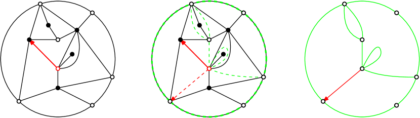
Figure 11: Tutte’s bijection applied to a truncated hull of even radius, here of radius 2. In every face of $Q$ of degree 4 but the external one, draw a “diagonal” between the two white corners. Then erase the edges of the original map and all black vertices, keeping however the edges of the boundary. The map we obtain is rooted at the edge drawn in the face of $Q$ on the left of the root edge of $Q$, oriented in such a way that its tail vertex is the root vertex of $Q$.

6.1 Downward paths

In this section, we define certain special paths called downward paths, in the image of a quadrangulation of the cylinder under Tutte’s correspondence. These special paths will be used to derive upper bounds for the distances in the uipm.

Let $R>0$ be an integer, let $Q$ be a quadrangulation of the cylinder of height $2R$ with top boundary length $p$, and let $u_{0}$ be a vertex of its top boundary. We write $(u_{i})_{0\leq i<p}$ for the vertices of the top boundary in clockwise order, and extend this numbering to $i\in\mathbb{Z}$ by periodicity (recall that the top face is drawn as the infinite face). Recall that for every $i\in\mathbb{Z}$, the edge $\{u_{i},u_{i+1}\}$ is also an edge of ${\mathcal{T}\left(Q\right)}$.

Recall the skeleton decomposition from Section 2: $Q$ is encoded by a forest $(\tau_{i})_{0\leq i<p}$, whose vertices are identified with the edges of $\partial_{r}q$ for $0\leq r\leq 2R$, and a collection of truncated quadrangulations. We extend the numbering of the forest to $\mathbb{Z}$ by periodicity, and shift the indices so that for all $i\in\mathbb{Z}$, the left-most vertex of the root of $\tau_{i}$ is $u_{i}$.

We say that the vertex $u_{i}$ is good if the slot associated with the edge $(u_{i},u_{i+1})$ is filled in by the truncated quadrangulation represented in the right side of Figure 12 (in particular the edge $(u_{i},u_{i+1})$ must have exactly one child in the skeleton), and bad otherwise. Assume that at least one of the $u_{j}$’s is labeled good, and let $u_{i}$, with $-p\leq i\leq-1$, be the first good vertex visited when exploring the top boundary in counterclockwise order starting from $u_{-1}$. We define the downward path $\operatorname{DP}(u_{0},2R-2)$ from $u_{0}$ to $\partial_{2R-2}Q$ as follows. We first move along $\partial_{2R}Q$ in counterclockwise order from $u_{0}$ to $u_{i}$. Then, we follow the unique edge of ${\mathcal{T}\left(Q\right)}$ from $u_{i}$ to $\partial_{2R-2}q$ inside the slot associated with $(u_{i},u_{i+1})$. See Figure 12 for an illustration.

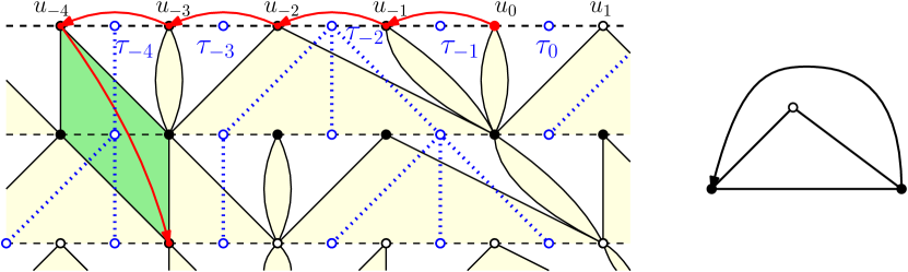
Figure 12: Left, a part of the annulus $\mathcal{C}(2R-2,2R)$ with slots in pale yellow, the skeleton in dotted blue lines, and the special slot in green. We have not drawn the edges and vertices inside the other slots. The downward path (in red) visits $u_{0},u_{-1},u_{-2},\ldots$ until it meets a “good” vertex (here $u_{-4})$, whose corresponding slot is filled by the truncated quadrangulation on the right side.

This path can be extended by induction to a path in ${\mathcal{T}\left(Q\right)}$ from $u_{0}$ to $\partial_{2s}Q$ for every $0\leq s<2R$, provided we can find good vertices at height $2k$ for all $s<k\leq R$. If not, the downward path is not defined, but we still define its length to be $+\infty$.

We can extend this definition to downward paths in ${\mathcal{T}\left(\mathcal{L}\right)}$ where $\mathcal{L}$ is the lhpq with truncated boundary. There will a.s. be good vertices at all heights, thus downward paths are always well defined.

The following lemma provides an upper bound on the length of downward paths in annuli of the uipq (recall that these annuli are quadrangulations of the cylinder). Roughly speaking, this upper bound shows that the graph distance (in ${\mathcal{T}\left(Q_{\infty}\right)}$) between a vertex of $\partial_{2s}Q_{\infty}$ and the cycle $\partial_{2r}Q_{\infty}$ is not larger than a constant times $s-r$, with high probability uniformly in $r<s<R$.

Lemma 25.

We can find $\alpha>0$ such that the following holds. For every $\varepsilon,\delta>0$ and every integer $R>0$, let $A_{R}(\delta,\varepsilon)$ be the event where for all $\delta\frac{R}{\ln R}\leq r<s\leq R$ such that $s-r\geq\varepsilon r$, for every $v\in\partial_{2s}Q_{\infty}$, the downward path from $v$ to $\partial_{2r}Q_{\infty}$ is well defined and has length smaller than $\alpha(s-r)$. Then

$$\mathbb{P}(A_{R}(\delta,\varepsilon))\underset{R\to\infty}{\longrightarrow}1.$$

Proof.

We fix an integer $R>0$. Let us first consider a forest $(\widetilde{\tau}_{1},\widetilde{\tau}_{2},...,\widetilde{\tau}_{p})$ of $p$ independent Bienaymé-Galton-Watson trees with offspring distribution $\theta$, where $R<p\leq R^{3}$. We truncate this forest at generation $2R$ (we remove all vertices whose height is greater than $2R$). We can view this forest as the skeleton of a quadrangulation $\widetilde{Q}$ of the cylinder whose height is the maximal generation in the truncated forest (in the skeleton decomposition of $\widetilde{Q}$, slots are filled in independently according to the same distribution as in the uipq). We again say that a vertex $u$ of the skeleton is good if it has a unique child and the slot corresponding to $u$ is filled as shown in the right side of Figure 12. We let $a>0$ be the product of $\theta(1)$ with the probability that a slot with lower boundary of size $1$ is filled in as just explained. Informally, $a$ represents the probability that a vertex is good.

Let $T$ stand for the smallest $i\geq 0$ such that generation $2i$ has no good vertex. For every $i\geq 0$, let $Y_{i}$ be the number of vertices at generation $2i$, and

$$\zeta=\min\{i:Y_{i}\leq R\text{ or }Y_{i}>R^{3}\}.$$

Note that, on the event $\{\zeta>R\}$, the height of the truncated forest is $2R$ and $\widetilde{Q}$ is a quadrangulation of the cylinder of height $2R$. For every $i\geq 0$, let $\mathcal{F}_{i}$ be the $\sigma$-field generated by the trees truncated at generation $2i$ and the labels good or bad up to generation $2i-2$ (the labels at generation $2i$ are not $\mathcal{F}_{i}$-measurable).

Fix a vertex $u$ at generation $0$ in the forest. For every $1\leq i\leq T$, we can construct the downward path from $u$, or rather from the vertex $v$ of $\widetilde{Q}$ which is the left end of the edge associated with $u$, to generation $2i$ of the forest (more precisely to the cycle whose edges form generation $2i$ of the forest), and we define $L_{u}(i)$ as the length of this downward path. By convention, $L_{u}(0)=0$.

Let us observe the following key fact: we can construct a sequence $G_{0},G_{1},...$ of i.i.d. geometric random variables with parameter $a$ such that, for every $0\leq i\leq R-1$,

$$\mathds{1}_{\left\{T\geq i\right\}}\mathbb{P}\left(L_{u}(i+1)-L_{u}(i)\neq G_{i}+2\ |\ \mathcal{F}_{i}\right)\leq\mathds{1}_{\left\{T\geq i\right\}}a^{Y_{i}}$$ (30)

(note that $\{T\geq i\}\in\mathcal{F}_{i}$). This bound holds because $\mathcal{F}_{i}$ gives no information on whether vertices at generation $2i$ are good or not: if these vertices are enumerated in clockwise order starting from a random vertex measurable w.r.t. $\mathcal{F}_{i}$ the index of the first good one will follow a geometric distribution “truncated” at $Y_{i}$.

Let us now bound, for $1\leq k\leq R$,

$$\mathbb{P}\left(T\geq k,\zeta\geq k\ ,\ L_{u}(k)\neq\sum_{i=0}^{k-1}(G_{i}+2)\right)$$

$$\leq \ \mathbb{P}\left(T\geq k,\zeta\geq k\ ,\ L_{u}(k-1)\neq\sum_{i=0}^{k-2}(G_{i}+2)\right)+\mathbb{P}\left(T\geq k,\zeta\geq k\ ,\ L_{u}(k)-L_{u}(k-1)\neq G_{k-1}+2\right)$$

$$\leq \ \mathbb{P}\left(T\geq k-1,\zeta\geq k-1\ ,\ L_{u}(k-1)\neq\sum_{i=0}^{k-2}(G_{i}+2)\right)+\mathbb{E}\left[\mathds{1}_{\left\{\zeta\geq k\right\}}a^{Y_{k-1}}\right],$$

using (30) and the property that $\{\zeta\geq k\}$ is $\mathcal{F}_{k-1}$-measurable. By induction, we get

$$\mathbb{P}\left(T\geq k,\zeta\geq k\ ,\ L_{u}(k)\neq\sum_{i=0}^{k-1}(G_{i}+2)\right)\leq\sum_{i=0}^{k-1}\mathbb{E}\left[\mathds{1}_{\left\{\zeta>i\right\}}a^{Y_{i}}\right]\leq ka^{R}.$$ (31)

We can similarly bound

$$\mathbb{P}\left(\zeta\geq k,T<k\right) =\sum_{i=0}^{k-1}\mathbb{P}(T=i,\zeta\geq k)$$

$$\leq\sum_{i=0}^{k-1}\mathbb{P}(T=i,\zeta>i)$$

$$=\sum_{i=0}^{k-1}\mathbb{E}\left[\mathds{1}_{\left\{T>i-1\right\}}\mathds{1}_{\left\{\zeta>i\right\}}a^{Y_{i}}\right]$$

where the last equality is obtained by conditioning with respect to $\mathcal{F}_{i}$ (on the event $\{T>i-1\}$, we have $\mathbb{P}(T=i\ |\ \mathcal{F}_{i})=a^{Y_{i}}$). It follows that

$$\mathbb{P}\left(\zeta\geq k,T<k\right)\leq ka^{R}.$$ (32)

On the other hand, by elementary large deviations estimates, there exist $\alpha,A>0$ such that for every $k\geq 0$,

$$\mathbb{P}\left(\sum_{i=0}^{k-1}(G_{i}+2)>\alpha k\right)\leq e^{-Ak}.$$ (33)

By combining (31) and (33), we arrive at

$$\mathbb{P}\left(T\geq k,\zeta\geq k\ ,\ L_{u}(k)>\alpha k\right)\leq ka^{R}+e^{-Ak}.$$

We apply this to $k=R-r$ for all values of $r$ such that $r\geq\delta\frac{R}{\ln R}$ and $R-r>\varepsilon r$, to get

$$\mathbb{P}\left(T\geq R-{\left\lceil\delta\frac{R}{\ln R}\right\rceil},\zeta\geq R-{\left\lceil\delta\frac{R}{\ln R}\right\rceil}\ ,\ L_{u}(R-r)>\alpha(R-r)\hbox{ for some }r\hbox{ s.t. }\delta\frac{R}{\ln R}\leq r<\frac{R}{1+\varepsilon}\right)$$

$$\quad\leq R^{2}a^{R}+R\,e^{-A\delta\frac{R}{\ln R}}.$$

We can then consider the union over all vertices $u$ at generation $0$ of the events appearing in the last display. Since generation $0$ has at most $R^{3}$ vertices, the probability of this union is trivially bounded by $R^{3}(R^{2}a^{R}+R\,e^{-A\delta R/\ln R})$.

Fix an integer $s$ such that $\frac{R}{\ln R}\leq r<s\leq R$. For every vertex $u$ at generation $2(R-s)$ in the forest and every $R-s\leq k\leq R$, we use the same notation $L_{u}(k)$ for the length of the downward path in $\widetilde{Q}$ from $u$ (or rather from the vertex $v$ of $\widetilde{Q}$ which is the left end of the edge associated with $u$) to $\partial_{2R-2k}\widetilde{Q}$ (corresponding to generation $2k$ in the forest coding $\widetilde{Q}$), provided this downward path exists. The same argument we used in the case $s=R$ shows that the probability of the event where $T\wedge\zeta\geq R-{\left\lceil\delta\frac{R}{\ln R}\right\rceil}$ and there exists a vertex $u$ at generation $2(R-s)$ such that $L_{u}(s-r)>\alpha(s-r)$ for some $r$ such that $\delta\frac{R}{\ln R}\leq r<s$ and $s-r\geq\varepsilon r$ is bounded above by

$$R^{3}(R^{2}a^{R}+R\,e^{-A\delta\varepsilon R/\ln R}).$$

We then sum this estimate over possible values of $s$. To simplify notation, set

$$\mathcal{R}(R,\delta,\varepsilon)=\left\{(r,s)\in\mathbb{N}\times\mathbb{N}\ :\ \delta\frac{R}{\ln R}\leq r<s\leq R,\ s-r\geq\varepsilon r\right\},$$

and also write $\mathcal{D}$ for the event where $L_{u}(R-r)<\alpha(s-r)$ for every $(r,s)\in\mathcal{R}(R,\delta,\varepsilon)$ and every vertex $u$ at generation $2(R-s)$ in the forest. Then using also (32) we get

$$\mathbb{P}\left(\left\{\zeta\geq R-\delta\frac{R}{\ln R}\right\}\cap\mathcal{D}^{c}\right)\leq Ra^{R}+R^{6}a^{R}+R^{5}e^{-A\varepsilon\delta R/\ln R}.$$ (34)

Consider now the uipq $Q_{\infty}$ and fix $\eta>0$. Using the tail estimates in Proposition 4, we can easily verify that for $R$ large enough, the event

$$\mathcal{E}\overset{\text{def}}{=}\bigcap_{{\left\lceil\delta\frac{R}{\ln R}\right\rceil}\leq r\leq R}\left\{R<H_{2r}\leq R^{3}\right\}.$$

has probability at least $1-\eta/2$. Let $A_{R}(\delta,\varepsilon)$ be the event considered in the statement of the lemma: $A_{R}(\delta,\varepsilon)$ is the event where, for every $(r,s)\in\mathcal{R}(R,\delta,\varepsilon)$, for every vertex $v$ of $\partial_{2s}Q_{\infty}$ the downward path from $v$ to $\partial_{2r}Q_{\infty}$ (exists and) has length smaller than $\alpha(s-r)$. We observe that the event

$$\mathcal{E}\cap A_{R}(\delta,\varepsilon)^{c}$$

is a function of the skeleton of the annulus $\mathcal{C}(2{\left\lceil\delta\frac{R}{\ln R}\right\rceil},2R)$ (and the quadrangulations filling in the slots). The point is now that the event in the left-hand side of (34) is the same function of the forest $(\widetilde{\tau}_{1},\widetilde{\tau}_{2},...,\widetilde{\tau}_{p})$ of independent trees truncated at height $2R-2{\left\lceil\delta\frac{R}{\ln R}\right\rceil}$ (and of the quadrangulations used to construct $\widetilde{Q}$ from its skeleton). This means that we can use the relations between the law of the skeleton of the annulus and that of a forest of independent trees to compare $\mathbb{P}(\mathcal{E}\cap A_{R}(\delta,\varepsilon)^{c})$ with the probability in (34). More precisely, Proposition 6 gives for every $R<p^{\prime}\leq R^{3}$,

$$\mathbb{P}\Big{(}\mathcal{E}\cap A_{R}(\delta,\varepsilon)^{c}\cap\left\{H_{2{\left\lceil\delta\frac{R}{\ln R}\right\rceil}}=p^{\prime}\right\}\Big{|}\ H_{2R}=p\Big{)}$$

$$\quad=\frac{\varphi_{2{\left\lceil\delta\frac{R}{\ln R}\right\rceil}}(p^{\prime})}{\varphi_{2R}(p)}\mathbb{P}\left(\left\{\zeta>R-\delta\frac{R}{\ln R}\right\}\cap\mathcal{D}^{c}\cap\left\{Y_{R-{\left\lceil\delta\frac{R}{\ln R}\right\rceil}}=p^{\prime}\right\}\right),$$ (35)

where we recall that $Y_{i}$ is the number of vertices at generation $2i$ in the forest $(\widetilde{\tau}_{1},\widetilde{\tau}_{2},...,\widetilde{\tau}_{p})$. Using the explicit formula (8), we find a constant $C>0$ such that for every sufficiently large $R$ and $p^{\prime}\leq R^{3}$,

$$\varphi_{2{\left\lceil\delta\frac{R}{\ln R}\right\rceil}}(p^{\prime}) \leq CR^{3}\left(\delta\frac{R}{\ln R}\right)^{-3}\leq C\delta^{-3}(\ln R)^{3}.$$

On the other hand, (8) and Proposition 4 give for $p^{\prime}>0$

$$\frac{\mathbb{P}(H_{2R}=p)}{\varphi_{2R}(p)}=\frac{32}{3\kappa_{1}}\frac{3+2R}{((3+2R)^{2}-1)^{2}}\kappa_{p}(2\pi_{2R})^{p}\left(\frac{64}{3}{p}\frac{3+2R}{((3+2R)^{2}-1)^{2}}\pi_{2R}^{{p}-1}\right)^{-1}=\frac{2^{p}\kappa_{p}}{{p}(2\kappa_{1})}\pi_{2R}\leq C^{\prime}$$

for a suitable constant $C^{\prime}$ independent of ${p}>0$. Multiplying (6.1) by $\mathbb{P}(H_{2R}={p})$ and summing over all choices of $R<p,{p^{\prime}}\leq R^{3}$ (using (34)), we get

$$\mathbb{P}\Big{(}\mathcal{E}\cap A_{R}(\delta,\varepsilon)^{c}\Big{)}\leq\left(C\delta^{-3}(\ln R)^{3}\right)\left(C^{\prime}R^{3}\right)\left(Ra^{R}+R^{6}a^{R}+R^{5}e^{-A\varepsilon\delta R/\ln R}\right),$$

which is smaller than $\eta/2$ for $R$ large. We already saw that the probability of $\mathcal{E}$ is larger than $1-\eta/2$ for $R$ large enough, so we get that for all $\eta>0$, for $R$ large enough $\mathbb{P}(A_{R}(\delta,\varepsilon))\geq 1-\eta$. This completes the proof. ∎

6.2 Coalescence in the UIPM

Downward paths do not coalesce as nicely as left-most geodesics, but we can still get an ersatz of Proposition 15. Let $R>0$ an integer. Choose a vertex $u_{0}^{(R)}$ uniformly distributed over $\partial_{2R}Q_{\infty}$, write $(u_{j}^{(R)})_{0\leq j\leq H_{2R}-1}$ for the vertices of $\partial_{2R}Q_{\infty}$ enumerated in clockwise order, and extend the definition of $u_{j}^{(R)}$ to all $j\in\mathbb{Z}$ by periodicity.

Corollary 26 (Coalescence of downward paths).

For every $\varepsilon>0$ and $\eta\in(0,1)$, we can find a constant $A>1$ such that, for every large enough integer $R$, the following holds with probability at least $1-\varepsilon$: any vertex of $\partial_{2R}Q_{\infty}$ is connected to one of the vertices $u_{{\left\lfloor kR^{2}/A\right\rfloor}}^{(R)}$, $0\leq k\leq{\left\lfloor AH_{2R}/R^{2}\right\rfloor}$, by a path in ${\mathcal{T}\left(\mathcal{C}(2R-2{\left\lceil\eta R\right\rceil},2R)\right)}$ of length at most $\eta R$.

Proof.

Consider two integers $0<s<R$. In the same way as we defined the downward path from a vertex $v$ of $\partial_{2R}Q_{\infty}$ to $\partial_{2s}Q_{\infty}$, we can define the dual notion of the right downward path from $v$ to $\partial_{2s}Q_{\infty}$: If $v=u^{(R)}_{j}$, the first step goes from $v$ to $u^{(R)}_{j+1}$, then we move clockwise along $\partial_{2R}Q_{\infty}$ until we meet a good vertex which allows us to go in one step from $\partial_{2R}Q_{\infty}$ to $\partial_{2(R-2)}Q_{\infty}$, and we continue by induction. As in the case of downward paths, the existence of the right downward path requires the existence of at least one good vertex on every cycle $\partial_{2j}Q_{\infty}$, $s<j\leq R$.

Let $v,w$ be two distinct vertices of $\partial_{2R}Q_{\infty}$ and let $0<s<R$. Assume that the downward paths (and right downward paths) from $v$ and $w$ to $\partial_{2s}Q_{\infty}$ are well defined, and furthermore that the left-most geodesics from $v$ and from $w$ coalesce (strictly) before reaching $\partial_{2s}Q_{\infty}$. Write $\mathcal{L}$ for the union of these two left-most geodesics up to their coalescence time, and $\mathcal{C}_{1}$, resp. $\mathcal{C}_{2}$, for the path from $v$ to $w$ along $\partial_{2R}Q_{\infty}$ in clockwise order, resp. in counterclockwise order. Let $\mathcal{R}_{1}$, resp. $\mathcal{R}_{2}$, be the (closed) bounded region delimited by the closed path which is the union of $\mathcal{L}$ and $\mathcal{C}_{1}$, resp. the union of $\mathcal{L}$ and $\mathcal{C}_{2}$. Then either $\mathcal{R}_{1}$ or $\mathcal{R}_{2}$ does not intersect $\partial_{2s}Q_{\infty}$. Consider the first case for definiteness, so that $\mathcal{R}_{1}$ is contained in the annulus between $\partial_{2R}Q_{\infty}$ and $\partial_{2s}Q_{\infty}$. Then our construction shows that the downward path starting from $w$ can only exit $\mathcal{R}_{1}$ after hitting the left-most geodesic started from $v$ (informally a downward path cannot cross a left-most geodesic “from left to right” — for this property to hold, it is important that we started our downward paths with a “horizontal” step). Similarly, the right downward path started from $v$ can only exit $\mathcal{R}_{1}$ after hitting the left-most geodesic started from $w$. A planarity argument now shows that the downward path started from $w$ and the right downward path started from $v$ intersect before exiting $\mathcal{R}_{1}$, and therefore before hitting $\partial_{2s}Q_{\infty}$. Consequently, $v$ and $w$ are connected by a path in ${\mathcal{T}\left(\mathcal{C}(2R-2{\left\lceil\eta R\right\rceil},2R)\right)}$ whose length is bounded by the sum of the lengths of the downward path from $w$ to $\partial_{2s}Q_{\infty}$ and the right downward path from $v$ to $\partial_{2s}Q_{\infty}$

Let $\alpha$ be as given in Lemma 25. Without loss of generality we can assume $\alpha\geq 1$. We apply the preceding considerations with $s=s(R)=R-{\left\lceil\eta R/(3\alpha)\right\rceil}$. Using also Lemma 25, we get that, if $R$ is large enough, the following holds with probability at least $1-\varepsilon/2$: Whenever $v$ and $w$ are two vertices of $\partial_{2R}Q_{\infty}$ such that the left-most geodesics from $v$ and from $w$ coalesce before reaching $\partial_{2s}Q_{\infty}$, $v$ and $w$ are connected by a path of ${\mathcal{T}\left(\mathcal{C}(2s,2R)\right)}$ of length at most $2\alpha(R-s)\leq\eta R$.

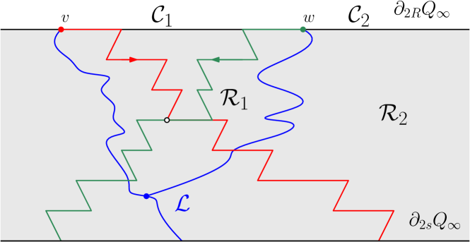
Figure 13: In blue, the left-most geodesics (in $Q_{\infty}$) started from $v,w$ two vertices of $\partial_{2R}Q_{\infty}$, that coalesce before reaching $\partial_{2s}Q_{\infty}$. The downward path in ${\mathcal{T}\left(Q_{\infty}\right)}$ started at $w$ (in green) cannot cross the left-most geodesic in $Q_{\infty}$ from $w$, and the right downward path in ${\mathcal{T}\left(Q_{\infty}\right)}$ started at $v$ (in red) cannot cross the left-most geodesic in $Q_{\infty}$ from $v$: by planarity, they must cross (and thus intersect) before reaching $\partial_{2s}Q_{\infty}$. We get a path in ${\mathcal{T}\left(Q_{\infty}\right)}$ between $v$ and $w$ by first following the right downward path from $v$ up to the intersection (white point), then the (reverse) downward path from $w$.

On the other hand, Proposition 15 yields $A>0$ such that with probability at least $1-\varepsilon/2$, any left-most geodesics starting from a vertex of $\partial_{2R}Q_{\infty}$ coalesces before reaching $\partial_{2s(R)}Q$ with one of the left-most geodesics started from $u_{{\left\lfloor kR^{2}/A\right\rfloor}}$, $0\leq k\leq{\left\lfloor AH_{2R}/(2R)^{2}\right\rfloor}$. By combining this with the preceding paragraph, we get that, with probability at least $1-\varepsilon$, any vertex of $\partial_{2R}Q_{\infty}$ is connected to one of these vertices $u_{{\left\lfloor kR^{2}/A\right\rfloor}}$ by a path of ${\mathcal{T}\left(\mathcal{C}(2s,2R)\right)}$ of length at most $\eta R$. This completes the proof. ∎

6.3 Two technical lemmas

We prove an estimate on the maximum degree of an inner face in the image of a large truncated hull of $Q_{\infty}$ by Tutte’s correspondence. We then obtain a bound on the first-passage percolation distance in ${\mathcal{T}\left(Q_{\infty}\right)}$ between a vertex of $\partial_{2n}Q_{\infty}$ and the root vertex, for $n$ large enough.

Lemma 27.

For every integer $r\geq 1$, let $\Delta^{\circ}\left({\mathcal{T}\left(\mathcal{H}^{\text{tr}}_{Q_{\infty}}(2r)\right)}\right)$ denote the maximal degree of internal faces of ${\mathcal{T}\left(\mathcal{H}^{\text{tr}}_{Q_{\infty}}(2r)\right)}$.

$$\mathbb{P}\left(\Delta^{\circ}\left({\mathcal{T}\left(\mathcal{H}^{\text{tr}}_{Q_{\infty}}(2r)\right)}\right)>5\ln r\right)\underset{r\to\infty}{\longrightarrow}0.$$

Proof.

For any map $M$, let $\Delta(M)$ be the maximal degree of a face of $M$. Let $M_{n}$ be a uniform rooted map with $n$ edges. It follows from [8, Theorem 3] that

$$\mathbb{P}(\Delta(M_{n})>\ln n)\underset{n\to\infty}{\longrightarrow}0.$$ (36)

This result is actually stated for the maximal degree of a vertex of $M_{n}$ in [8], but (36) then follows by self-duality of $M_{n}$, see [3, Lemma 3.2].

By Proposition 20 we can fix an integer $A>0$ large enough such that, for every $r$ large enough, we can couple $Q^{\bullet}_{{\left\lfloor Ar^{4}\right\rfloor}}$ and $Q_{\infty}$ so that $B^{\bullet}_{Q^{\bullet}_{{\left\lfloor Ar^{4}\right\rfloor}}}(2r)=B^{\bullet}_{Q_{\infty}}(2r)$ except on a set of probability at most $\varepsilon/2$. Note that this equality of hulls also implies $\mathcal{H}^{\text{tr}}_{Q^{\bullet}_{{\left\lfloor Ar^{4}\right\rfloor}}}(2r)=\mathcal{H}^{\text{tr}}_{Q_{\infty}}(2r)$ (the truncated hull is determined by the “standard” hull). Thus on the latter event,

$$\Delta^{\circ}\left({\mathcal{T}\left(\mathcal{H}^{\text{tr}}_{Q_{\infty}}(2r)\right)}\right)=\Delta^{\circ}\left({\mathcal{T}\left(\mathcal{H}^{\text{tr}}_{Q^{\bullet}_{{\left\lfloor Ar^{4}\right\rfloor}}}(2r)\right)}\right)\leq\Delta\left({\mathcal{T}\left(Q_{{\left\lfloor Ar^{4}\right\rfloor}}\right)}\right).$$

To get the last inequality, we observe that the degree of an internal face of $\mathcal{T}(\mathcal{H}^{\text{tr}}_{Q^{\bullet}_{{\left\lfloor Ar^{4}\right\rfloor}}}(2r))$ is exactly the degree of the black vertex of $\mathcal{H}^{\text{tr}}_{Q^{\bullet}_{{\left\lfloor Ar^{4}\right\rfloor}}}(2r)$ that is contained in this face, and this vertex has the same degree in $\mathcal{H}^{\text{tr}}_{Q^{\bullet}_{{\left\lfloor Ar^{4}\right\rfloor}}}(2r)$ and in $Q_{{\left\lfloor Ar^{4}\right\rfloor}}$. See Figure 11.

We know that ${\mathcal{T}\left(Q_{{\left\lfloor Ar^{4}\right\rfloor}}\right)}$ is distributed as $M_{{\left\lfloor Ar^{4}\right\rfloor}}$. To complete the proof, we note that (36) ensures that for $r$ large enough, $\Delta\left(M_{{\left\lfloor Ar^{4}\right\rfloor}}\right)\leq 5\ln r$ with probability at least $1-\varepsilon/2$. ∎

Lemma 28.

For every $\varepsilon>0$, there exists $A>0$ such that for all $n$ large enough,

$$\mathbb{P}\left(\max_{v\in\partial_{2n}Q_{\infty}}\mathrm{d}_{\mathrm{fpp}}^{{\mathcal{T}\left(Q_{\infty}\right)}}(\rho,v)\leq 2An\right)\geq 1-\varepsilon.$$

Proof.

Since weights are bounded, it is enough to prove this statement with $\mathrm{d}_{\mathrm{fpp}}^{{\mathcal{T}\left(Q_{\infty}\right)}}$ replaced by $\mathrm{d}_{\mathrm{gr}}^{{\mathcal{T}\left(Q_{\infty}\right)}}$. Let $\eta\in(0,1)$. To simplify notation, in the remaining part of the proof, we write $H_{n}=\mathcal{H}^{\text{tr}}_{Q_{\infty}}\left(2{\left\lfloor\eta\frac{n}{\ln n}\right\rfloor}\right)$ so that $\partial H_{n}=\partial_{2{\left\lfloor\eta\frac{n}{\ln n}\right\rfloor}}Q_{\infty}$.

By Lemma 25, if $n$ is large enough, we have with probability at least $1-\varepsilon/2$

$$\mathrm{d}_{\mathrm{gr}}^{{\mathcal{T}\left(Q_{\infty}\right)}}\left(v,\partial H_{n}\right)\leq\alpha n,$$

for every $v\in\partial_{2n}Q_{\infty}$. On the other hand, by Lemma 27 the bound $\Delta^{\circ}\left({\mathcal{T}\left(H_{n}\right)}\right)\leq 5\ln n$ holds with probability at least $1-\varepsilon/2$ when is large. On this event, the simple bound

$$\mathrm{d}_{\mathrm{gr}}^{{\mathcal{T}\left(H_{n}\right)}}(x,y)\leq\Delta^{\circ}\left({\mathcal{T}\left(H_{n}\right)}\right)\mathrm{d}_{\mathrm{gr}}^{H_{n}}(x,y),$$

valid for all $x,y\in V\left({\mathcal{T}\left(H_{n}\right)}\right)$, ensures that for all $v\in\partial H_{n}$, $\mathrm{d}_{\mathrm{gr}}^{{\mathcal{T}\left(Q_{\infty}\right)}}(\rho,v)\leq 10\eta n$. The statement of the lemma follows by combining these observations. ∎

6.4 Continuity properties of the Tutte correspondence

Let us use the notation $M_{n}={\mathcal{T}\left(Q_{n}\right)}$ for the image of $Q_{n}$ under Tutte’s bijection. Note that $M_{n}$ is uniformly distributed over (rooted) planar maps with $n$ edges. For every $r>0$, we write $\mathcal{B}_{M_{n}}(r)$ for the (closed) metric ball of radius $r$ centered at the root vertex $\rho_{n}$ in $V(M_{n})$. We may view this ball (resp. its complement) as a graph by keeping only those edges incident to a face of the ball (resp. of its complement).

Proposition 29.

For every $\varepsilon,\eta>0$, there exists $\delta>0$ s.t. for all $n$ large enough,

$$\mathbb{P}\left(\sup_{x\in V(M_{n}),\ \mathrm{d}_{\mathrm{gr}}^{Q_{n}}(\rho_{n},x)\leq\delta n^{1/4}}\mathrm{d}_{\mathrm{gr}}^{M_{n}}(\rho_{n},x)\leq\varepsilon n^{1/4}\right)\geq 1-\eta.$$

Proof.

We again use the convergence in distribution to the Brownian map $({\text{m}_{\infty}},D^{*})$. It follows from (28) that we can choose a constant $K>2$ large enough so that, for every $\varepsilon>0$, the probability of the event where at least two connected components of the complement of the ball $\mathcal{B}_{\text{m}_{\infty}}(\varepsilon)$ intersect the complement of $\mathcal{B}_{\text{m}_{\infty}}(K\varepsilon/2)$ is bounded above by $\eta/4$. From [3, Corollary 1.2], we know that the random compact metric spaces $(V(M_{n}),(\frac{9}{8n})^{1/4}\mathrm{d}_{\mathrm{gr}}^{M_{n}})$ converge in distribution in the Gromov-Hausdorff sense to the Brownian map. Although this is not stated in [3], it follows from the proof that this convergence also holds in the pointed Gromov-Hausdorff sense, if $M_{n}$ is pointed at the root vertex $\rho_{n}$ (and ${\text{m}_{\infty}}$ is pointed at $x_{*}$). From this pointed convergence, and the properties of the Brownian map stated above, we can now deduce that, for every $\varepsilon>0$, for all sufficiently large $n$, the probability that at least two components of the complement of the ball $\mathcal{B}_{M_{n}}(\varepsilon n^{1/4})$ intersect the complement of the ball $\mathcal{B}_{M_{n}}(K\varepsilon n^{1/4})$ is bounded above by $\eta/2$.

Let us fix $\varepsilon>0$ and set $\beta=\varepsilon/K$. We can assume that $\varepsilon$ is so small that $\mathbb{P}(\mathrm{d}_{\mathrm{gr}}^{Q_{n}}(\rho_{n},\partial_{n})>4K\beta n^{1/4})>1-\eta/4$. Using the coupling between $Q_{n}^{\bullet}$ and the uipq $Q_{\infty}$ in Proposition 20, we get from Lemma 28 that there exists $\mu>0$ such that

$$\max_{v\in\partial_{2{\left\lfloor\mu n^{1/4}\right\rfloor}}Q_{n}^{\bullet}}\mathrm{d}_{\mathrm{gr}}^{M_{n}}(\rho_{n},v)<\frac{\beta}{2}n^{1/4}$$

with probability at least $1-\eta/4$. Recall that the edges of the cycle $\partial_{2{\left\lfloor\mu n^{1/4}\right\rfloor}}Q^{\bullet}_{n}$ are also edges of $M_{n}$. Argue on the event where both the bound in the last display holds and $\mathrm{d}_{\mathrm{gr}}^{Q_{n}}(\rho_{n},\partial_{n})>4K\beta n^{1/4}$. Then, except on an event of probability at most $\eta/2$, at most one of the two components bounded by the cycle $\partial_{2{\left\lfloor\mu n^{1/4}\right\rfloor}}Q^{\bullet}_{n}$ can intersect the complement of the ball $\mathcal{B}_{M_{n}}(K\beta n^{1/4})$, and this must be the component that contains the distinguished vertex $\partial_{n}$. We conclude that, except on a set of probability at most $\eta$, the truncated hull $\mathcal{H}^{\text{tr}}_{Q^{\bullet}_{n}}(2{\left\lfloor\mu n^{1/4}\right\rfloor})$ does not intersect the complement of the ball $\mathcal{B}_{M_{n}}(K\beta n^{1/4})$, and in particular the bound

$$\sup_{x\in V(M_{n}),\ \mathrm{d}_{\mathrm{gr}}^{Q_{n}}(\rho_{n},x)\leq 2{\left\lfloor\mu n^{1/4}\right\rfloor}}\mathrm{d}_{\mathrm{gr}}^{M_{n}}(\rho_{n},x)\leq K\beta n^{1/4}=\varepsilon n^{1/4}$$

holds with probability at least $1-\eta$. This completes the proof. ∎

7 Main results for general maps

7.1 Subadditivity in the LHPQ

Recall from the beginning of Section 6 that we can apply Tutte’s bijection to the lhpq $\mathcal{L}$, and that ${\mathcal{T}\left(\mathcal{L}\right)}$ denotes the resulting infinite map. We observe that every edge of the form $((i,-2r),(i+1,-2r))$ for $r\geq 0$ and $i\in\mathbb{Z}$ appear in ${\mathcal{T}\left(\mathcal{L}\right)}$ because vertices of the type $(i,-2r)$ are white, and every edge of the preceding form is a diagonal of some quadrangle. It follows that we can define slices of ${\mathcal{T}\left(\mathcal{L}\right)}$ for even coordinates in a way similar to the case of the lhpq: for even $j\leq j^{\prime}\leq 0$, ${\mathcal{T}\left(\mathcal{L}\right)}_{j}^{j^{\prime}}$ is the part of ${\mathcal{T}\left(\mathcal{L}\right)}$ contained in $\mathbb{R}\times[j,j^{\prime}]$. Furthermore, disjoint slices are independent.

We write $\mathrm{d}_{\mathrm{fpp}}^{\mathcal{T}\left(\mathcal{L}\right)}(x,y)$, for $x,y\in V({\mathcal{T}\left(\mathcal{L}\right)})$, for the first-passage percolation distance on $V({\mathcal{T}\left(\mathcal{L}\right)})$ (recall that weights belong to $[1,\kappa]$).

Proposition 30.

There exists a constant $\textbf{c}_{T}\in[\frac{1}{2},\infty)$ such that

$$(2r)^{-1}\mathrm{d}_{\mathrm{fpp}}^{\mathcal{T}\left(\mathcal{L}\right)}(\rho,\partial_{-2r}\mathcal{L})\overset{\text{a.s.}}{\underset{r\to\infty}{\longrightarrow}}\textbf{c}_{T}.$$ (37)

Proof.

The proof uses the same subadditivity argument as that of Proposition 13, with the minor difference that we restrict our attention to even heights.

We first note that, for $x,y\in V({\mathcal{T}\left(\mathcal{L}\right)})$, $\mathrm{d}_{\mathrm{fpp}}^{\mathcal{T}\left(\mathcal{L}\right)}(x,y)\geq\mathrm{d}_{\mathrm{gr}}^{\mathcal{T}\left(\mathcal{L}\right)}(x,y)\geq\frac{1}{2}\mathrm{d}_{\mathrm{gr}}^{\mathcal{L}}(x,y)$, so that the limit $\textbf{c}_{T}$ in (37), if it exists, has to be greater than or equal to $1/2$. The only new part is that we have to check that $\mathbb{E}[\mathrm{d}_{\mathrm{gr}}^{\mathcal{T}\left(\mathcal{L}\right)}(\rho,\partial_{-2}\mathcal{L})]<\infty$.

As we already noticed in Section 6.1, the downward path started from the root is well defined in the lhpq, and provides an upper bound on $\mathrm{d}_{\mathrm{gr}}^{\mathcal{T}\left(\mathcal{L}\right)}(\rho,\partial_{-2}\mathcal{L})$. The number of steps of this downward path before it reaches a vertex of $\partial_{-2}\mathcal{L}$ is distributed as $G+2$, where $G$ is a geometric random variable, thus has a finite expectation, giving the desired result. ∎

7.2 Distance through a thin annulus

We use the notation $M_{\infty}={\mathcal{T}\left(Q_{\infty}\right)}$, so that $M_{\infty}$ may be called the uniform infinite planar map or uipm.

Proposition 31.

Let $\varepsilon\in(0,1)$ and $\delta>0$. For every $\eta>0$ small enough, for all sufficiently large $n$, the property

$$2(1-\varepsilon)\textbf{c}_{T}\eta n\leq\mathrm{d}_{\mathrm{fpp}}^{M_{\infty}}(v,\partial_{2(n-{\left\lfloor\eta n\right\rfloor})}Q_{\infty})\leq 2(1+\varepsilon)\textbf{c}_{T}\eta n,$$ (38)

holds for every $v\in\partial_{2n}Q_{\infty}$, with probability at least $1-\delta$.

Proof.

The proof is patterned after that of Proposition 16 using Proposition 30 instead of Proposition 13. The following minor adaptations are required.

Let $u^{(n)}_{0}$ be a uniformly distributed vertex of $\partial_{2n}Q_{\infty}$. Then Lemma 25 ensures that we have with high probability,

$$\mathrm{d}_{\mathrm{fpp}}^{M_{\infty}}\left(u^{(n)}_{0},\partial_{2(n-{\left\lfloor\eta n\right\rfloor})}Q_{\infty}\right)\leq 2\alpha\kappa{\left\lfloor\eta n\right\rfloor}.$$

Let $\mathcal{G}^{(n)}_{0}$ be defined as in the proof of Proposition 16 (with $n$ replaced by $2n$). As in the latter proof, we know with high probability that the length of the minimal path (in $Q_{\infty}$) between $u^{(n)}_{0}$ and the lateral boundary of $\mathcal{G}^{(n)}_{0}$ that stays in $\widetilde{\mathcal{H}}^{\mathrm{tr}}_{Q_{\infty}}(2n)$ is bounded below by $cn$ with some constant $c>0$. Trivially, two vertices of ${\mathcal{H}}^{\mathrm{tr}}_{Q_{\infty}}(2n)$ that are linked by an edge of ${\mathcal{T}\left(Q_{\infty}\right)}$ are also connected by a $Q_{\infty}$-path of length two in $\widetilde{\mathcal{H}}^{\mathrm{tr}}_{Q_{\infty}}(2n)$. Taking $\eta$ smaller if necessary, it follows that the $\mathrm{d}_{\mathrm{fpp}}^{M_{\infty}}$-shortest path between $u^{(n)}_{0}$ and $\partial_{2(n-{\left\lfloor\eta n\right\rfloor})}Q_{\infty}$ that stays in ${\mathcal{H}}^{\mathrm{tr}}_{Q_{\infty}}(2n)$ does not leave $\mathcal{G}^{(n)}_{0}$ on an event of high probability. We can then use the same density arguments as in the proof of Proposition 16.

In the last step of the proof, we need to verify that it suffices to obtain (38) for a bounded number of vertices $v$ of $\partial_{2n}Q_{\infty}$. The argument is the same as in the proof of Proposition 16, but we use Corollary 26 in place of Proposition 15. ∎

7.3 Distance from the boundary of a hull to its center

The next proposition is analogous to Proposition 17.

Proposition 32.

For every $\varepsilon\in(0,1)$,

$$\mathbb{P}\left(2(\textbf{c}_{T}-\varepsilon)n\leq\mathrm{d}_{\mathrm{fpp}}^{M_{\infty}}(\rho,v)\leq 2(\textbf{c}_{T}+\varepsilon)n\ \text{ for every }v\text{ in }\partial_{2n}Q_{\infty}\right)\underset{n\to\infty}{\longrightarrow}1.$$

Proof.

The proof is very similar to that of Proposition 17. Consider the annuli $\mathcal{C}(2n_{k+1},2n_{k})$ for every $0\leq k<q$, where $n_{0}=n$ and $n_{k+1}=n_{k}-{\left\lfloor\eta n_{k}\right\rfloor}$, and $q$ is as defined in Proposition 17. By Proposition 31, we can find $\eta>0$ such that “most” of these annuli will satisfy the analog of (38), except possibly on a set of probability at most $\varepsilon$. We then use Lemma 25 to bound the $\mathrm{d}_{\mathrm{fpp}}^{M_{\infty}}$-distance through the annuli where (38) does not hold, and Lemma 28 to control the $\mathrm{d}_{\mathrm{fpp}}^{M_{\infty}}$-distance between $\rho$ and $\partial_{2n_{q}}Q_{\infty}$. ∎

7.4 Distance between two uniformly sampled points in finite maps

Recall that $M_{n}={\mathcal{T}\left(Q_{n}\right)}$ in such a way that $V(M_{n})$ can be viewed as the subset of $V(Q_{n})$ consisting of the “white” vertices. Also recall that $\#V(Q_{n})=n+2$. We observe that

$$\frac{\#V(M_{n})}{\#V(Q_{n})}\underset{n\to\infty}{\longrightarrow}\frac{1}{2}$$

in probability (see e.g. the proof of Proposition 3.1 in [3]). Then, since conditionally on $Q_{n}$ the distinguished vertex $\partial_{n}$ is uniformly distributed over $V(Q_{n})$, we have also

$$\mathbb{P}(\partial_{n}\in V(M_{n}))\underset{n\to\infty}{\longrightarrow}\frac{1}{2}.$$

We also observe that the result of Proposition 29 remains valid if we replace the root vertex $\rho_{n}$ by $\partial_{n}$. More precisely, for every $\varepsilon,\eta>0$, we can find $\beta>0$ such that, for all $n$ large enough, we have

$$\mathbb{P}\left(\sup_{x\in V(M_{n}),\ \mathrm{d}_{\mathrm{gr}}^{Q_{n}}(\partial_{n},x)\leq\beta n^{1/4}}\mathrm{d}_{\mathrm{gr}}^{M_{n}}(\partial_{n},x)\leq\varepsilon n^{1/4}\Bigg{|}\,\partial_{n}\in V(M_{n})\right)\geq 1-\eta.$$ (39)

This follows from the invariance of $Q_{n}$ under uniform re-rooting, by an argument very similar to the one used in the proof of Theorem 22.

Proposition 33.

For every $\gamma\in(0,1)$,

$$\mathbb{P}\left(|\mathrm{d}_{\mathrm{fpp}}^{M_{n}}(\rho_{n},\partial_{n})-\textbf{c}_{T}\mathrm{d}_{\mathrm{gr}}^{Q_{n}}(\rho_{n},\partial_{n})|>\gamma n^{1/4}\,\Big{|}\,\partial_{n}\in V(M_{n})\right)\underset{n\to\infty}{\longrightarrow}0.$$

Proof.

The proof is based on the same ingredients as that of Proposition 18, but we use Proposition 32, or rather (39), instead of Proposition 17. We argue on the event where $\partial_{n}\in V(M_{n})$. Let $\gamma>0$, $\eta>0$ and choose $\beta>0$ so that (39) holds with $\varepsilon=\gamma$.

Fix $\delta>0$ small enough so that $3\delta^{2}<\beta$ and the event $H_{n,\delta}$ of Lemma 21 has probability at least $1-\eta$ when $n$ is large. For integers $j,l\geq 1$, let $H_{n,\delta}^{j,l}$ be defined as in Lemma 21. If $n$ is large, the $\mathrm{d}_{\mathrm{gr}}^{Q_{n}}$-distance between $\partial_{n}$ and $\partial_{2{\left\lfloor\alpha_{j}n^{1/4}/2\right\rfloor}}Q^{\bullet}_{n}$ is smaller than $\beta n^{1/4}$ on $H_{n,\delta}^{j,l}$. Thus, on the intersection of $H_{n,\delta}^{j,l}$ with the event considered in (39) (with $\varepsilon=\gamma$), the $\mathrm{d}_{\mathrm{gr}}^{M_{n}}$-distance between $\partial_{n}$ and $\partial_{2{\left\lfloor\alpha_{j}n^{1/4}/2\right\rfloor}}Q^{\bullet}_{n}$ is smaller that $\gamma n^{1/4}$.

On the other hand, from Proposition 32 and using (23) as in the proof of Proposition 18, we get that, outside of a set of probability going to $0$ as $n\to\infty$, the $\mathrm{d}_{\mathrm{fpp}}^{M_{n}}$-distance between any vertex of $\partial_{2{\left\lfloor\alpha_{j}n^{1/4}/2\right\rfloor}}Q^{\bullet}_{n}$ and $\rho_{n}$ is close to $\textbf{c}_{T}\alpha_{j}n^{1/4}$, up to an error term bounded by $\gamma n^{1/4}$.

Finally, on the intersection of $H_{n,\delta}$ with $\{\partial_{n}\in V(M_{n})\}$ and with the event considered in (39), we have

$$|d(\rho_{n},\partial_{n})-\textbf{c}_{T}\mathrm{d}_{\mathrm{gr}}^{Q^{\bullet}_{n}}(\rho_{n},\partial_{n})|\leq(1+\kappa)\gamma n^{1/4},$$

except on a set of probability tending to $0$ as $n\to\infty$. Using Lemma 21 we obtain that the latter intersection has probability larger than $\mathbb{P}(\partial_{n}\in V(M_{n}))-2\eta$ for all $n$ large enough. This completes the proof. ∎

7.5 Distances between any pair of points of finite maps

The next statement gives both Theorem 2 and the part of Theorem 1 concerning general planar maps.

Theorem 34.

For every $\varepsilon>0$, we have

$$\mathbb{P}\left(\sup_{x,y\in V(M_{n})}\left|\mathrm{d}_{\mathrm{fpp}}^{M_{n}}(x,y)-\textbf{c}_{T}\mathrm{d}_{\mathrm{gr}}^{Q_{n}}(x,y)\right|>\varepsilon n^{1/4}\right)\underset{n\to\infty}{\longrightarrow}0$$

If all weights are equal to $1$ (that is, $\mathrm{d}_{\mathrm{fpp}}^{M_{n}}=\mathrm{d}_{\mathrm{gr}}^{M_{n}}$), we have $\textbf{c}_{T}=1$.

Before we prove Theorem 34, we state and prove a lemma.

Lemma 35.

Let $\eta\in(0,1)$, and, for every $n\geq 1$, conditionally on $M_{n}$, let $\partial_{n}^{1},\partial_{n}^{2},\ldots$ be independent random vertices uniformly distributed over $V(M_{n})$. Then, for every $\varepsilon>0$, we can find an integer $N\geq 1$ such that, for every sufficiently large $n$, we have

$$\mathbb{P}\left(\max_{v\in V(M_{n})}\,\left(\min_{1\leq\ell\leq N}\mathrm{d}_{\mathrm{gr}}^{M_{n}}(\partial^{\ell}_{n},v)\right)<\varepsilon\,n^{1/4}\right)>1-\eta.$$

Proof.

We first note that the statement would follow if we knew the convergence in the Gromov-Hausdorff-Prokhorov sense of $(V(M_{n}),(9/8n)^{1/4}\mathrm{d}_{\mathrm{gr}}^{M_{n}})$ equipped with the uniform probability measure to the Brownian map — cf. the analogous statement for $Q_{n}$ used in the proof of Theorem 22. Unfortunately, [3] does not give the Gromov-Hausdorff-Prokhorov convergence, and so we will provide a direct proof, which still relies much on the arguments of [3]. We start by observing that [3, Proposition 3.1] allows us to replace $M_{n}$ by a random pointed planar map $M_{n}^{\bullet}$ which is uniformly distributed over pointed planar maps with $n$ edges (this replacement needs to be justified because, in contrast with the case of quadrangulations, forgetting the distinguished vertex of $M_{n}^{\bullet}$ does not give a map distributed as $M_{n}$). Then, as in [3, Section 4], we can construct a finite sequence $\widetilde{v}^{n}_{0},\widetilde{v}^{n}_{1},\ldots,\widetilde{v}^{n}_{2n}$ such that every vertex $v$ of $M_{n}^{\bullet}$ appears at least once in this sequence, and, if we set $\widetilde{D}_{n}(i,j)=\mathrm{d}_{\mathrm{gr}}^{M_{n}^{\bullet}}(\widetilde{v}^{n}_{i},\widetilde{v}^{n}_{i})$ for $i,j\in\{0,1,\ldots,2n\}$ and interpolate linearly to get a function $\widetilde{D}(s,t)$ defined on $[0,2n]^{2}$, we have

$$\left(\left(\frac{9}{8n}\right)^{1/4}\widetilde{D}_{n}(2ns,2nt)\right)_{0\leq s,t\leq 1}\underset{n\to\infty}{\longrightarrow}(D^{*}(s,t))_{0\leq s,t\leq 1},$$

in distribution in the space of continuous functions on $[0,1]^{2}$. Here $D^{*}(s,t)$ is the random pseudo-metric on $[0,1]^{2}$ that defines the Brownian map. Since $D^{*}$ vanishes on the diagonal, we can fix an integer $A\geq 1$ such that, writing $\delta=1/A$, the property

$$D^{*}(s,s^{\prime})<\frac{\varepsilon}{4}\;,\qquad\forall s,s^{\prime}\in[(k-1)\delta,k\delta],\;\forall k\in\{1,\ldots,A\}$$

holds with probability greater than $1-\eta/2$. Using the preceding convergence, it follows that, for $n$ large enough, the property

$$\mathrm{d}_{\mathrm{gr}}^{M_{n}^{\bullet}}(\widetilde{v}^{n}_{i},\widetilde{v}^{n}_{j})<\frac{\varepsilon}{2}\,n^{1/4}\;,\qquad\forall i,j\in[2n(k-1)\delta,2nk\delta]\cap\mathbb{Z},\;\forall k\in\{1,\ldots,A\}$$

also holds with probability greater than $1-\eta/2$. We claim that we can find an integer $N$ large enough so that, for every $n$ large enough, with probability greater than $1-\eta/2$, there exists for each $k\in\{1,\ldots,A\}$ an index $\ell\in\{1,\ldots,N\}$ and an integer $i\in[2n(k-1)\delta,2nk\delta]$ such that

$$\mathrm{d}_{\mathrm{gr}}^{M_{n}^{\bullet}}(\partial_{n}^{\ell},\widetilde{v}^{n}_{i})\leq\frac{\varepsilon}{2}\,n^{1/4}.$$

If we combine the claim with the preceding considerations, we get that, with probability at least $1-\eta$, any vertex of $M_{n}^{\bullet}$ is at distance smaller than $\varepsilon n^{1/4}$ from one of the vertices $\partial_{n}^{\ell}$, $\ell\in\{1,\ldots,N\}$, which was the desired result.

It remains to prove our claim. To this end, we need more information about the sequence $\widetilde{v}^{n}_{i}$ (we refer to [3] for more details). Via the Ambjørn-Budd bijection, the pointed planar map $M^{\bullet}_{n}$ is associated with a (uniformly distributed) pointed quadrangulation $Q^{\bullet}_{n}$ with $n$ faces, in such a way that $V(M^{\bullet}_{n})$ is identified to a subset of $V(Q^{\bullet}_{n})$, and in particular $\#V(M^{\bullet}_{n})\leq\#V(Q^{\bullet}_{n})=n+2$. In the CVS correspondence, $V(Q^{\bullet}_{n})$ corresponds to a labeled tree $T_{n}$, and the contour sequence $v^{n}_{0},v^{n}_{1},\ldots,v^{n}_{2n}$ of the tree $T_{n}$ (defined as in the proof of Lemma 21) can also be viewed as a sequence of vertices of $Q^{\bullet}_{n}$. Then, for every $i\in\{1,\ldots,2n\}$, $v^{n}_{i}$ and $\widetilde{v}^{n}_{i}$ are linked by an edge of $Q^{\bullet}_{n}$ (see [3]). Moreover, in the case when $v^{n}_{i}\in V(M^{\bullet}_{n})$, one has

$$\mathrm{d}_{\mathrm{gr}}^{M^{\bullet}_{n}}(v^{n}_{i},\widetilde{v}^{n}_{i})\leq\Delta(M^{\bullet}_{n}).$$ (40)

This bound follows directly from the construction of the Ambjørn-Budd bijection (the point is that any edge of $Q^{\bullet}_{n}$ is contained in a face of $M^{\bullet}_{n}$). Recalling (36), and using again [3, Proposition 3.1], we know that we have $\Delta(M^{\bullet}_{n})<\frac{\varepsilon}{2}n^{1/4}$ with probability greater than $1-\eta/8$. For every integer $p\in\{0,1,\ldots,n\}$, let $\mathcal{N}^{(n)}_{p}$ be the number of distinct vertices $v^{n}_{i}$ with $i\in\{0,1,\ldots,p\}$ that belong to $V(M^{\bullet}_{n})$. Then, from the end of [3, Section 5], we have for every $t\in[0,1]$,

$$\frac{1}{n}\,\mathcal{N}^{(n)}_{{\left\lfloor 2nt\right\rfloor}}\underset{n\to\infty}{\longrightarrow}\frac{t}{2}$$

in probability. It follows that, for $n$ large enough, we have

$$\#\{v^{n}_{i}:i\in[2n(k-1)\delta,2nk\delta]\hbox{ and }v^{n}_{i}\in V(M^{\bullet}_{n})\}\geq\mathcal{N}^{(n)}_{{\left\lfloor 2nk\delta\right\rfloor}}-\mathcal{N}^{(n)}_{\lceil 2n(k-1)\delta\rceil}\geq\frac{\delta}{4}\,n\;,\ \forall k\in\{0,1,\ldots,A\},$$ (41)

with probability at least $1-\eta/8$. We can choose $N$ large enough so that, on the event (41), the conditional probability given $M_{n}^{\bullet}$ that each set $\{v^{n}_{i}:i\in[2n(k-1)\delta,2nk\delta]\hbox{ and }v^{n}_{i}\in M^{\bullet}_{n}\}$, for $1\leq k\leq A$, contains at least one of the vertices $\partial_{n}^{\ell}$, $1\leq\ell\leq N$, is greater than $1-\eta/4$. Summarizing the preceding considerations and using (40), we get that, with probability at least $1-\eta/2$, for every $k\in\{1,\ldots,A\}$, there exist an index $\ell\in\{1,\ldots,N\}$ and an integer $i\in[2n(k-1)\delta,2nk\delta]$ such that $\partial_{n}^{\ell}=v^{n}_{i}$ and $\mathrm{d}_{\mathrm{gr}}^{M^{\bullet}_{n}}(\partial_{n}^{\ell},\widetilde{v}^{n}_{i})=\mathrm{d}_{\mathrm{gr}}^{M^{\bullet}_{n}}(v^{n}_{i},\widetilde{v}^{n}_{i})<\frac{\varepsilon}{2}n^{1/4}$. This completes the proof of the claim and of the lemma. ∎

Proof of Theorem 34.

By the same re-rooting invariance argument as in the proof of Theorem 22, the statement of Proposition 33 remains valid if the pair $(\rho_{n},\partial_{n})$ is replaced by $(\partial^{\prime}_{n},\partial^{\prime\prime}_{n})$, where, conditionally on $Q_{n}$, $\partial^{\prime}_{n}$ and $\partial^{\prime\prime}_{n}$ are independent and uniformly distributed over $V(Q_{n})$: more precisely, we have, for every $\varepsilon>0$,

$$\mathbb{P}\left(|\mathrm{d}_{\mathrm{fpp}}^{M_{n}}(\partial^{\prime}_{n},\partial^{\prime\prime}_{n})-\textbf{c}_{T}\mathrm{d}_{\mathrm{gr}}^{Q_{n}}(\partial^{\prime}_{n},\partial^{\prime\prime}_{n})|>\varepsilon n^{1/4}\,\Big{|}\,\partial^{\prime}_{n}\in V(M_{n}),\partial^{\prime\prime}_{n}\in V(M_{n})\right)\underset{n\to\infty}{\longrightarrow}0.$$

Let us fix $\varepsilon>0$ and $\eta>0$. Thanks to Lemma 35, we can fix an integer $N$ large enough so that, if $\partial^{1}_{n},\partial^{2}_{n},\ldots,\partial^{N}_{n}$ are independent and uniformly distributed over $V(M_{n})$, then, with probability at least $1-\eta$, the metric balls of radius $\varepsilon n^{1/4}$ in $(V(M_{n}),\mathrm{d}_{\mathrm{gr}}^{M_{n}})$ centered at $\partial^{1}_{n},\ldots,\partial^{N}_{n}$ cover $V(M_{n})$. Let us call $\mathcal{H}_{n}$ the event where this covering property holds.

On the other hand, consider the event

$$\mathcal{K}_{n}:=\{|\mathrm{d}_{\mathrm{fpp}}^{M_{n}}(\partial^{i}_{n},\partial^{j}_{n})-\textbf{c}_{T}\mathrm{d}_{\mathrm{gr}}^{Q_{n}}(\partial^{i}_{n},\partial^{j}_{n})|\leq\varepsilon n^{1/4},\;\forall i,j\in\{1,\ldots,N\}\}.$$

By the first observation of the proof, we have also $\mathbb{P}(\mathcal{K}_{n})\geq 1-\eta$ for $n$ large enough.

For $n$ large, the event $\mathcal{H}_{n}\cap\mathcal{K}_{n}$ has probability at least $1-2\eta$. Let us argue on this event in the remaining part of the proof. Let $x,y\in V(M_{n})$, we can find $i,j\in\{1,\ldots,N\}$ such that $\mathrm{d}_{\mathrm{gr}}^{M_{n}}(\partial^{i}_{n},x)\leq\varepsilon n^{1/4}$ and $\mathrm{d}_{\mathrm{gr}}^{M_{n}}(\partial^{j}_{n},y)\leq\varepsilon n^{1/4}$. Note that this implies $\mathrm{d}_{\mathrm{gr}}^{Q_{n}}(\partial^{i}_{n},x)\leq 2\varepsilon n^{1/4}$ and $\mathrm{d}_{\mathrm{gr}}^{Q_{n}}(\partial^{j}_{n},y)\leq 2\varepsilon n^{1/4}$. It follows that we have

$$|\mathrm{d}_{\mathrm{fpp}}^{M_{n}}(x,y)-\mathrm{d}_{\mathrm{fpp}}^{M_{n}}(\partial^{i}_{n},\partial^{j}_{n})|\leq\mathrm{d}_{\mathrm{fpp}}^{M_{n}}(\partial^{i}_{n},x)+\mathrm{d}_{\mathrm{fpp}}^{M_{n}}(\partial^{j}_{n},y)\leq 2\kappa\varepsilon n^{1/4}$$

and

$$|\mathrm{d}_{\mathrm{gr}}^{Q_{n}}(x,y)-\mathrm{d}_{\mathrm{gr}}^{Q_{n}}(\partial^{i}_{n},\partial^{j}_{n})|\leq 4\varepsilon n^{1/4}.$$

Hence, from the definition of $\mathcal{K}_{n}$,

$$|\mathrm{d}_{\mathrm{fpp}}^{M_{n}}(x,y)-\textbf{c}_{T}\mathrm{d}_{\mathrm{gr}}^{Q_{n}}(x,y)|\leq(1+4\textbf{c}_{T}+2\kappa)\varepsilon\,n^{1/4}.$$

This completes the proof of the first assertion.

As for the second one, we observe that the first assertion, together with the known convergence of rescaled quadrangulations to the Brownian map, implies that

$$\left(V(M_{n}),{\left(\frac{9}{8n}\right)}^{1/4}\mathrm{d}_{\mathrm{fpp}}^{M_{n}}\right)\overset{\textrm{(d)}}{\underset{n\to\infty}{\longrightarrow}}({\text{m}_{\infty}},\textbf{c}_{T}D^{*})$$

in distribution in the Gromov-Hausdorff sense. In the case where all weights are equal to $1$, comparing this convergence with [3, Corollary 1.2] gives $c_{T}=1$. ∎

7.6 Distances in the UIPM

Recall that $M_{\infty}={\mathcal{T}\left(Q_{\infty}\right)}$ is the uipm.

Theorem 36.

Let $\varepsilon\in(0,1)$. We have

$$\lim_{r\to\infty}\mathbb{P}\left(\sup_{x,y\in V(M_{\infty}),\,\mathrm{d}_{\mathrm{gr}}^{M_{\infty}}(\rho,x)\vee\mathrm{d}_{\mathrm{gr}}^{M_{\infty}}(\rho,y)\leq r}\left|\mathrm{d}_{\mathrm{fpp}}^{M_{\infty}}(x,y)-\textbf{c}_{T}\mathrm{d}_{\mathrm{gr}}^{M_{\infty}}(x,y)\right|>\varepsilon r\right)=0,$$ (42)

and

$$\lim_{r\to\infty}\mathbb{P}\left(\sup_{x,y\in V(M_{\infty}),\,\mathrm{d}_{\mathrm{gr}}^{M_{\infty}}(\rho,x)\vee\mathrm{d}_{\mathrm{gr}}^{M_{\infty}}(\rho,y)\leq r}\left|\mathrm{d}_{\mathrm{gr}}^{M_{\infty}}(x,y)-\mathrm{d}_{\mathrm{gr}}^{Q_{\infty}}(x,y)\right|>\varepsilon r\right)=0.$$ (43)

We only sketch the proof, as it is very similar to that of Theorem 23. Since $\mathrm{d}_{\mathrm{gr}}^{M_{\infty}}(x,y)\geq\frac{1}{2}\mathrm{d}_{\mathrm{gr}}^{Q_{\infty}}(x,y)$ for every $x,y\in V(M_{\infty})$, the condition $\mathrm{d}_{\mathrm{gr}}^{M_{\infty}}(\rho,x)\leq r$ implies $\mathrm{d}_{\mathrm{gr}}^{Q_{\infty}}(\rho,x)\leq 2r$. By the same argument, we can find a constant $K$ large enough so that, for every $r\geq 1$ and for every $x,y\in V(M_{\infty})$ such that $\mathrm{d}_{\mathrm{gr}}^{M_{\infty}}(\rho,x)\leq r$ and $\mathrm{d}_{\mathrm{gr}}^{M_{\infty}}(\rho,y)\leq r$, the quantities $\mathrm{d}_{\mathrm{fpp}}^{M_{\infty}}(x,y)$, $\mathrm{d}_{\mathrm{gr}}^{M_{\infty}}(x,y)$ and $\mathrm{d}_{\mathrm{gr}}^{Q_{\infty}}(x,y)$ are determined by the hull $B^{\bullet}_{Q_{\infty}}(Kr)$ (and of course weights on edges in the case of $\mathrm{d}_{\mathrm{fpp}}^{M_{\infty}}$). We then use Proposition 20 that allows us to find a large constant $C$ such that the hulls $B^{\bullet}_{Q^{\bullet}_{{\left\lfloor C(Kr)^{4}\right\rfloor}}}(Kr)$ and $B^{\bullet}_{{Q_{\infty}}}(Kr)$ are equal with probability close to $1$. We conclude by using Theorem 34.

Theorem 3 stated in the introduction follows from Theorem 23 and Theorem 36.

References

- [1] Céline Abraham et al. Rescaled bipartite planar maps converge to the brownian map. In Ann. Inst. Henri Poincaré Probab. Stat., volume 52, pages 575–595. Institut Henri Poincaré, 2016.
- [2] Louigi Addario Berry and Marie Albenque. The scaling limit of random simple triangulations and random simple quadrangulations. Ann. Probab., 45(5):2767–2825, 2017.
- [3] Jérémie Bettinelli, Emmanuel Jacob, and Grégory Miermont. The scaling limit of uniform random plane maps, via the Ambjørn–Budd bijection. Electron. J. Probab., 19, 2014.
- [4] Nicolas Curien, Tom Hutchcroft, and Asaf Nachmias. Geometric and spectral properties of causal maps. J. Eur. Math. Soc. (JEMS), to appear.
- [5] Nicolas Curien and Jean-François Le Gall. The Brownian plane. J. Theoret. Probab., 27(4):1249–1291, 2014.
- [6] Nicolas Curien and Jean-François Le Gall. First-passage percolation and local modifications of distances in random triangulations. Ann. Sci. Éc. Norm. Supér.(4), to appear.
- [7] Nicolas Curien, Laurent Ménard, and Grégory Miermont. A view from infinity of the uniform infinite planar quadrangulation. Lat. Am. J. Probab. Math. Stat. (ALEA), 10(1):45–88, 2013.
- [8] Zhicheng Gao and Nicholas C Wormald. The distribution of the maximum vertex degree in random planar maps. J. Combin. Theory Ser. A, 89(2):201–230, 2000.
- [9] Svante Janson and Jean-François Marckert. Convergence of discrete snakes. J. Theoret. Probab., 18(3):615–645, 2005.
- [10] Maxim Krikun. Local structure of random quadrangulations. arXiv:math/0512304v2, 2008.
- [11] Jean-François Le Gall and Thomas Lehéricy. Separating cycles and isoperimetric inequalities in the uniform infinite planar quadrangulation. Ann. Probab., 2017.
- [12] Jean-François Le Gall. Geodesics in large planar maps and in the brownian map. Acta Math., 205(2):287–360, 2010.
- [13] Jean-François Le Gall. Brownian disks and the Brownian snake. In Ann. Inst. Henri Poincaré Probab. Stat., volume 55, pages 237–313. Institut Henri Poincaré, 2019.
- [14] Jean-François Le Gall et al. Uniqueness and universality of the Brownian map. Ann. Probab., 41(4):2880–2960, 2013.
- [15] Jean-François Le Gall, Grégory Miermont, et al. Scaling limits of random trees and planar maps. Probability and statistical physics in two and more dimensions, 15:155–211, 2012.
- [16] Thomas M Liggett. An improved subadditive ergodic theorem. Ann. Probab., pages 1279–1285, 1985.
- [17] Laurent Ménard, Pierre Nolin, et al. Percolation on uniform infinite planar maps. Electron. J. Probab., 19, 2014.
- [18] Grégory Miermont. The Brownian map is the scaling limit of uniform random plane quadrangulations. Acta Math., 210(2):319–401, 2013.