Simultaneous state estimation and control for nonlinear systems subject to bounded disturbances
Abstract
In this work, we address the output–feedback control problem for nonlinear systems under bounded disturbances using a moving horizon approach. The controller is posed as an optimization-based problem that simultaneously estimates the state trajectory and computes future control inputs. It minimizes a criterion that involves finite forward and backward horizon with respect the unknown initial state, measurement noises and control input variables and it is maximized with respect the unknown future disturbances. Although simultaneous state estimation and control approaches are already available in the literature, the novelty of this work relies on linking the lengths of the forward and backward windows with the closed-loop stability, assuming detectability and decoding sufficient conditions to assure system stabilizability. Simulation examples are carried out to compare the performance of simultaneous and independent estimation and control approaches as well as to show the effects of simultaneously solving the control and estimation problems.
keywords:
Receding horizon control and estimation , Output feedback , Robust stability , Nonlinear systems., , ,
1 Introduction
One of the most popular control technique in both academia and industry is model predictive control (MPC) due to its ability to explicitly accommodate hard state and input constraints (Bemporad & Morari, 1999; Camacho & Alba, 2004; Rawlings & Mayne, 2009; Mayne, 2014, among others). Thereon, much effort has been devoted to developing a stability theory for MPC (see i.e. Rawlings & Mayne, 2009; Grüne & Pannek, 2011; Mayne, 2016). An overview of recent developments can be found in Mayne (2014). MPC involves the solution of an open–loop optimal control problem at each sampling time with the current state as the initial condition. Each of these optimizations provides the sequences of future control actions and states. The first element of the control action sequence is applied to the system and, then the optimization problem is solved again at the next sampling time after updating the initial condition with the system state. MPC keeps constant the computational burden by optimizing the system behaviour within a finite length window. The system behaviour beyond the window is summarized in a term known as cost–to–go.
MPC is often formulated assuming that the system state can be measured. However, in many practical cases, the only information available is noisy measurements of system output, so the use of independent algorithms for state estimation (including observers, filters and estimators) becomes necessary (see Rawlings & Bakshi, 2006). Of all these methods, moving horizon estimation (MHE) is especially engaging for use with MPC because it can be formulated as a similar online optimization problem. Solving the MHE problem produces an estimated state that is compatible with a set of past measurements that recedes as current time advances (Schweppe, 1973; Rao et al., 2001, 2003). This estimate is optimal in the sense that it maximizes a criterion that captures the likelihood of the measurements. Along the same time that relevant results on MPC were developed, research works on MHE begun. The works of Rao et al. (2001) and (2003) provide overviews of linear and nonlinear MHE. Recent results regarding MHE for nonlinear systems are given for robust stability and estimate convergence properties (see Alessandri et al., 2005, 2008, 2012; Garcia-Tirado et al., 2016; Sánchez et al., 2017, among others). In recent years several results have been obtained for different MHE formulations, advancing from idealistic assumptions, like observability and vanishing disturbances, to realistic situations like detectability and bounded disturbances (see Ji et al., 2015; Müller, 2017; Allan & Rawlings, 2019; Deniz et al., 2019).
When disturbances, model uncertainty and system constraints can be neglected, state and control sequences can be independently computed (see Duncan & Varaiya, 1971; Bensoussan, 2004; Åström, 2012; Georgiou & Lindquist, 2013). However, in practical applications, these conditions are very difficult to fulfil, i.e., process disturbances and measurement noise are usually present, as well as model uncertainty. In this context, it becomes necessary approaches that include this information into the controller design. State-feedback MPC is a mature field with results that considers model uncertainty, input disturbances, and noises (Magni et al., 2003; Bemporad et al., 2003; Raimondo et al., 2009, among others). However, these works did not consider robustness with respect to errors in state estimation. Fewer results are available for output-feedback MPC. An overview of nonlinear output-feedback MPC is given by Findeisen et al. (2003) and the references therein. Many of these approaches involve designing separate estimator and controller, using different estimation algorithm (Roset et al., 2006; Magni et al., 2009; Patwardhan et al., 2012; Zhang & Liu, 2013; Ellis et al., 2017). Results on robust output-feedback MPC for constrained, linear, discrete-time systems with bounded disturbances and measurement noise can be found in Mayne et al. (2006, 2009) and Voelker et al. (2010, 2013). These approaches first solve the estimation problem and prove the convergence of the estimated state to a bounded set, and then take the uncertainty of the estimation into account when solving the MPC problem.
The approach of solving simultaneously MHE–MPC was originally introduced by Copp & Hespanha (2014) and later developed in several papers (Copp & Hespanha, 2016a, b, 2017). In the first paper, Copp & Hespanha (2014) proposed an output feedback controller that combines state estimation and control into a single optimization problem that, under observability and controllability assumptions (Copp & Hespanha, 2016a), guarantees the boundedness of state and tracking errors. Finally, in the last work reported by Copp & Hespanha (2017), the authors established the conditions for guaranteeing the boundedness of error for trajectory tracking problems. They also introduced a primal–dual interior point method that can be used to efficiently solve the optimization problem. The criterion used in these works involves finite forward and backward horizons that are minimized with respect to feedback control policies and maximized with respect to the unknown parameters in order to guaranty robustness in the worst-case scenario.
In the present work, we introduce an output–feedback controller for nonlinear systems subject to bounded disturbances using simultaneous MHE–MPC approach. The resulting optimization problem minimizes a criterion that involves finite forward and backward horizons with respect the unknown initial state, measurement noise and control input variables while it is maximized with respect the unknown future disturbance variables. We show that the proposed controller results in closed–loop trajectories along which the states remain bounded. These results rely on two assumptions: The first assumption requires that the optimization criterion include an adaptive arrival cost (Sánchez et al., 2017). This assumption allows to ensure the boundedness of the state estimate and to obtain a bound for the estimation error set if the parameters of the estimation problem are properly chosen (Deniz et al., 2019). The second assumption requires that the backward (estimation) and forward (control) horizons are sufficiently large so that enough information is obtained in order to find state estimates and control inputs compatible with dynamics, noises and constraints. This assumption is satisfied if the system is detectable, stabilizable and the parameters in the cost function (weights and horizons) are chosen appropriately.
The rest of the paper is organized as follows: Section 2 introduces the notation, definitions and properties that will be used through the paper. In Section 3 we formulate the estimation and control problem, and in Section 4 we analyze its closed-loop stability. Section 5 discusses two examples to illustrate the concepts presented in this work. The first example uses a simple nonlinear model to analyse the consequences of simultaneously solving the estimation and control problems. The second example compares the performance obtained by the simultaneous and independent approaches applied to the regulation of the state of a van der Pol oscillator for two operational conditions. Finally, conclusion and future work is discussed in Section 6.
2 Preliminaries and setup
2.1 Notation
Let denotes the integer numbers, denotes the set of integers in the interval , with and denotes the set of integers greater or equal to . Boldface symbols denote sequences of finite () or infinite () length. We denote as the state at time estimated at time . By we denote the euclidean norm of a vector . Let denote the supreme norm of the sequence and . A function is of class if is continuous, strictly increasing and . If is also unbounded, it is of class . A function is of class if is continuous, non increasing and . A function is of class if is of class for each fixed , and of class for each fixed . Let us consider now two sets and , the Minkowski addition is defined as . On the other hand, the Minkowski difference111Also known as the Pontryagin difference. is defined as . In the following sections, we will use the notation to reference the cost incurred solving the problem p at time t with a horizon length l, while will be used to indicate the cost at the solution , with belonging to a consistent domain with the cost function . When necessary, we will use the notation and to differentiate –th component of the state vector of two discrete-time trajectories of the system, with . Moreover, will denote a trajectory with initial condition and perturbed by the sequence . A similar notation is used for the case of continuous time systems, where is used instead to denote continuous time.
2.2 Problem statement
Let us consider a discrete-time nonlinear system whose behaviour is given
| (1) |
where is the system state, is the system’s input and is the unmeasured process disturbance posed as an additive input. The output of the system is and is the measurement noise. The function is assumed to be at least locally Lipschitz in its arguments, and the function is known to be a continuous function. The sets , , , and are assumed to be convex, containing the origin in its interior. The estimation and control problem attempts to simultaneously find the optimal state and the optimal sequence of control inputs which will steer the system to the desired operation zone. It is in an infinite-horizon optimization problem given by
| (2) |
Functions penalize large values of and , whereas penalize large values of the predicted state and control inputs . The function is assumed to take non–negative values and since it is subtracting in the objective function, process disturbances will tend to be maximized within the control window. When necessary, we will decompose the function into and which penalizes and , respectively. Problem (2) is valuable from a theoretical point of view since it guarantees the boundedness of the estimates and control actions provided the cost function is bounded, i.e., , , with . If functions , and are defined using a norm–, problem (2) would guarantee that the state and are , provided that noises and are also . This would mean that the closed-loop system has a finite –induced gain.
The infinite–horizon problem (2) lacks practical interest since it is intractable from a computational point of view. Then, it is reformulated into a receding finite–horizon problem
| (3) |
For computation tractability, the infinite summations of have been replaced by backward and forward windows of finite length, corresponding to the estimation and control problems of criterion , respectively. includes terms backward in time from sample corresponding to the estimator stage-cost, , and the extra term , known as arrival-cost, that summarizes information left behind the estimation window by penalizing the uncertainty in the initial state (Rao et al., 2001, 2003). On the other hand, includes terms forward in time from sample corresponding to the controller stage-cost, , and an extra term , known as cost-to-go, that summarizes the behaviour of the system beyond the control window by penalizing the deviation of the final state . Moreover, the set represent the set of terminal constraints, as common in MPC (Rawlings et al., 2017).
The goal of problem (3) is to estimate the initial state and disturbances such that an estimate is obtained to compute the control inputs that drive the system states to the desired region. Therefore, there is no point on penalizing the control cost along the estimation window. The variables are not independent variables since they are uniquely determined by the remaining optimization variables and the output equation
| (4) |
Since there is no measurement of future system output, will not be considered along the control window. However, the disturbances needs to be considered along both windows and because they affect all the states, starting from . As will be shown later, the ratio between disturbances and control actions , for , encodes the controllability property of the system, imposing a bound on the relation between and in order to avoid to lose system controllability. However, in practical implementations, the process disturbance variables along the control horizon can be omitted to avoid increase the computational burden of the optimization problem.
Remark 1
The sequence of process disturbances is minimized within the estimator window, i.e., , and it is maximized within the controller window, .
2.3 Relationship with MHE and MPC
The criterion can be rewritten as follows
| (5) |
where is the criterion implemented by a MHE estimator and is to the criterion implemented by a robust MPC controller, given by
| (6) |
Equation (5) corresponds to a weighted sum multi-objective formulation of criterion (3), where controls the influence of on . When , and problem (3) becomes a robust model predictive control problem with terminal cost considered by Chen & Allgöwer (1998), given that is measurable or it is provided by an estimator. On the other case, when , and problem (3) becomes a moving horizon estimation problem considered by Ji et al. (2016); Garcia-Tirado et al. (2016); Müller (2017); Deniz et al. (2019), given that the control inputs are computed by a controller. In these cases, the optimization problem (3) has only one objective and the separation principle needs to be applied since the estimator and the controller are implemented independently.
When , and are simultaneously considered by and the optimization problem (3) becomes multi-objective. The importance of , and therefore the one of , is defined by emphasizing or deemphasizing the influence of the estimation problem on the solution. In the case of , and have similar influence on the solution of (3) and it becomes the problem proposed by Copp & Hespanha (2017).
Definition 1
Let assume points and such that . A point , is Pareto optimal iff there does not exist another point such that and , (Miettinen, 2012).
According to this concept, problem (3) looks for solutions that neither nor can be improved without deteriorate one of them. Any optimal solution of problem (3) with is Pareto optimal (Miettinen, 2012), therefore it has an optimal trade-off between and . On the other cases, or the solutions of problem (3) are optimal in the sense of the selected objective ( or , respectively). In these cases, the solutions obtained are not Pareto optimal and, therefore the overall system performance can be poorer than the one provided by the multi-objective problem.
From a practical point of view, can be used to improve the numerical properties of the optimization problem (3). This fact allows to improve the convergence properties of the numerical algorithms employed to solve it (see Example 4.2). For example, if and the stage costs and have similar values, the optimization problem will improve at the expense of (because ), deteriorating the estimation of and producing potentially ill conditioned Jacobian and Hessian matrices of . This numerical problems can lead to an increment of the computational times of the optimization problem. A similar situation can happen when .
3 Robust stability under bounded disturbances
In this section, we introduce the results regarding feasibility and robust stability of the proposed algorithm. Firstly, the properties of MHE and MPC are analyzed and then the results for the simultaneous MHE–MPC are given. Besides, feasibility conditions for the existence of a solution to (3) and minimum horizon lengths required to achieve the desired estimation and control performances are analyzed.
3.1 Backward window
The simultaneous state estimation and control problem relies on a backward window of fixed length to compute the optimal state estimate . Then, the controller takes the estimate as initial condition and predicts the system behaviour. To take advantage of the backward window and reconstruct the state of the system, there have to exists an observer for it, i.e., the system has to be detectable. A definition of detectability for nonlinear systems is incremental input-output-to-state stability -i-IOSS- (Sontag & Wang, 1995), and it entails that the difference between any two trajectories of the system can be bounded by
| (7) |
with , . In the following, we assume that the system is i-IOSS, i.e., any two trajectories eventually become indistinguishable one of another. Note that inequality (7) only includes the process disturbance as input to the system. For the case of non-autonomous system, as in the present work, control inputs also have to be taken into account. Since control inputs and process disturbances have the same nature in our context, considering both is straightforward. Moreover, as will be shown later in Example 4.1, the control law chosen have not only effects in the forward window but also in the backward window influencing on the estimation process.
Previous results on robust output-feedback MPC with bounded disturbances firstly solve the estimation problem and show the convergence of estimated states to a bounded set, then take the uncertainty of estimation into account when solving the MPC problem (Mayne et al., 2006, 2009). The key idea in these works was to consider the estimation error as an additional, unknown but bounded uncertainty that must be accounted for guaranteeing stability and feasibility of the resulting closed–loop system. Let us define the robust estimable set
| (8) |
where is the best estimate available and is the estimation error at time bounded by (Deniz et al., 2019)
| (9) |
Functions , and are defined in term of MHE parameters as follows
| (10) | ||||
| (11) | ||||
| (12) |
where , , , and are the minimal and maximal eigenvalues of the arrival-cost weight matrix , respectively. Moreover, the matrix is updated at each sampling time applying the algorithm developed in Sánchez et al. (2017). As in the case of the stage cost, the arrival–cost is lower and upper bounded by
| (13) |
On the other hand, , , , , , , , and are positive real constants whose value depend on the system and parameters of the estimator (Deniz et al., 2019). The functions and are related with the system detectability (equation (7)), whereas the functions and are bounds of the stage-cost of the estimator, whose relationship is given by
| (14) |
and is the length of the backward window. is the minimum length of the backward window required to guarantee the boundness of the estimation error, which is given by
| (15) |
where denotes the maximal error on the prior estimate of the initial condition and is a constant. Henceforth, we will assume that .
At each sampling time, the measurements available along the backward window are used to obtain . Whenever , the estimation error will decrease until it reaches an invariant space whose volume depends on the process and measurement noises as well as the stage- cost and the system itself. The behaviour of the system is forecast from the estimate , whereas remains within .
3.2 Forward window
The forward window corresponds to the MPC problem, which computes the optimal control inputs using as initial condition. Its feasibility depends on the fact that its initial condition must belong to the robust controllable set (Kerrigan & Maciejowski, 2000), which is defined as follows
| (16) |
Since the feasibility of the control problem is guaranteed if , which implies . Note that this feasibility condition is not only necessary for the simultaneous MHE–MPC, but also for independent MHE and MPC (Mayne et al., 2006, 2009). Let us state this condition in the following assumption
Assumption 1
The robust estimable set belong to the robust controllable set in steps for all times
| (17) |
This assumption states that despite the sequence of control is computed from an estimate , provided that belong to , . Moreover, the volume of the robust estimable set decrease faster with longer backward windows and the size of the robust controllable set can be enlarged by mean of larger forward window and with the appropriate design of the set .
Regarding stability along the forward window, a common approach to guarantee the stability of MPC is by mean of the inclusion of a terminal constraint set, which is generally a level set of a control Lyapunov function (Mayne et al., 2000). This set is an artificial constraint set but guarantees stability (Tuna et al., 2006). In this work we will analyse the stability of the controller following a similar approach as in Tuna et al. (2006), where the analysis is carried out as a function of the length of the forward window, taking into account the effect of the process disturbances and the estimation errors. A pseudo measure of the system controllability property will be introduced and the minimum forward window length which guarantees the stability of the simultaneous MHE–MPC is given, without imposing extra terminal constraints nor appeal for the cost-to-go to be a closed–loop Lyapunov function (CLF). In this sense, let us state the following assumption.
Assumption 2
There exist a constant such that the cost-to-go and the stage cost satisfy the following relation:
| (18) |
A similar assumption was already used in Tuna et al. (2006), where the constant is introduced in order to relax the requirement on function to be a CLF for the nominal case. Despite we use a different notation for the cost-to-go term , this function can take the same behaviour as the stage-cost, i.e., . Here we extend it to the more general case where process disturbances are affecting the system, and it will lead, as will be shown later, in longer control windows. However, in practical implementation, one can omit process disturbance optimization variables to avoid increasing the computational burden but setting the length of the forward window to the value computed with the process disturbance taken into account.
Regarding the elements of the optimization problem corresponding to the control problem, we will assume that the stage-cost is lower bounded.
Assumption 3
The stage cost is lower bounded by a function , such that .
Note that for a quadratic stage-cost, i.e., , with and positive definite matrices, one can choose , where denotes the minimal eigenvalue of matrix . Moreover, we will assume that there exist an increasing sequence that relates the function with the cost of the control problem , where represents different lengths of the forward window.
Assumption 4
There exists a sequence , , , that verifies
| (19) |
Choosing
| (20) |
satisfies inequality (19) even for , since . Finally, let us define the following quantity
| (21) |
It encodes a pseudo–measure of the system controllability relating the capability of control actions to compensate the process disturbances. The term pseudo–measure is used here because the relation is given via the penalization functions and . In the following, we will assume that the system is controllable from this point of view.
Assumption 5
The controller of the system can be designed such that the following relation can always be verified
| (22) |
With the properties established for the backward and forward windows in mind, next we will study the overall stability of the simultaneous MHE–MPC.
3.3 Backward and forward windows
With all the elements introduced in the previous section, we are ready to derive the main result: the stability of the resulting closed-loop system of the proposed output-feedback controller with estimation horizon and control horizon for nonlinear detectable and controllable systems under bounded disturbances.
Theorem 1
Given the i-IOSS nonlinear system (1) with a prior estimate of its unknown initial condition and bounded disturbances , , Assumptions 1 to 5 are fulfilled, the estimation window verifies and the control horizon verifies
| (23) |
then there will exist at each sampling time a feasible estimate and feasible sequences and such that
| (24) |
where
| (25) |
Proof. See Appendix A.
4 Examples
In this section, we discuss two examples to illustrate the results presented previously and compare the performance of the framework discussed formerly. The first example applies the ideas introduced in previous sections to a nonlinear scalar system. The emphasis is placed in the effect of constraints and disturbances on closed-loop stability and performance. The second example discusses the simulations results for a van der Pol oscillator using the framework discussed in previous sections. The discussion is focused on the effect of and on the performance and computational time.
4.1 Example 1
Let us consider the continuous–time nonlinear scalar system
| (26) |
Firstly, we show its detectability, i.e., the existence of an estimate with a structure like equation (7). Let assume two arbitrary and feasible trajectories and such that and ; then can be written as follows
| (27) |
Assuming a LTV control law , we obtain
| (28) |
which is upper bounded by
| (29) |
where
| (30) |
Solving for initial condition we obtain
| (31) |
it follows the fact that system (26) is i-IOSS (for all details, the reader can refer to appendix B).
In the case of MHE–MPC controllers with quadratic costs
| (32) |
analysed in this work, the bound (31) can be written as follows
| (33) |
with given by
| (34) |
and is the equivalent controller gain resulting from applying .
Equations (33) and (34) show the influence of the controller on the state estimation. Larger controller gains improve estimation error and shorten the convergence time. However, controller gains are bounded by robust stability conditions and input constraints, which are limiting factors in this potential improvement. This example highlights the relevance of simultaneously solving the estimation and control problems, or at least to take into account the solution of control problem on the estimation one. Since MPC gains are time-varying because they are recomputed at every sampling time, a conservative approach can employ its lowest value.
In order to compare the performances of independent and simultaneous MHE–MPC, both output–feedback controllers have the same parameters
| (35) |
with constraints sets
| (36) |
, , , and such that both controllers implement the same optimization criterion.
The control problems of both controllers are configured without terminal constraints. The process disturbance is not taken into account to compute but it will be considered in the computation of . It can be computed directly from equation (23) once the values of , and had been established. Another approach, employed in this example, consists of computing through simulations. In this example, we set the initial condition that maximizes the controller costs and then computes the values of and . The process is repeated until reach the maximal value of .
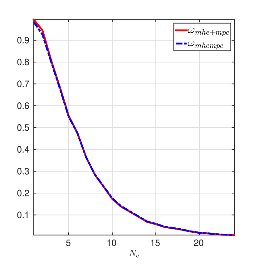
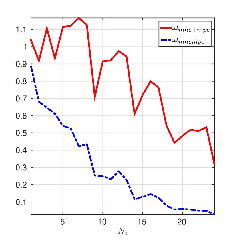
Figure 1 shows the computed values of a funtion of () for the same and different set of constraints and distributions for process and measurement noises. In this figure the effect of constraints on can be seen: They increase , for the same , depending how the controller is implemented. This change is smaller for the simultaneous MHE–MPC approach than the independent one. When constraints are no relevant (constraints set (36)), both controllers have similar values (see Figure 1(a)), and the control problem of both controllers can use the same . However when constraints are tighten (constraints set (37)), the way of solving the estimation and control problems has a direct effect on (see Figure 1(b)), and the control problem of both controllers must use different in order to ensure robust stability, affecting the computational requirements of the implementation. Since we are using constraints set (36) we choose for both controllers (Figure 1(a)). Finally, the minimum estimation horizon is computed from (15) using the parameters listed in (35), leading to for both controllers. We choose for both controllers.
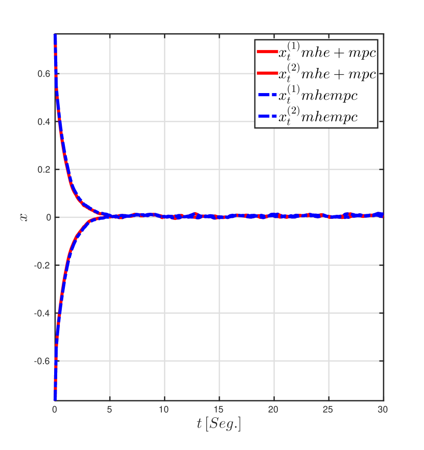
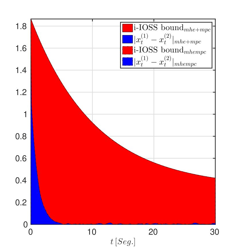
Figure 2 shows the system responses and the corresponding i-IOSS bound for the regulation problem. Figure 2(a) shows two trajectories generated by both controllers from different initial condition ( and ) with the same prior guess (). Figure 2(b) shows the difference between the trajectories and its i-IOSS bound, for the minimum controller gain along the simulation (). One can see in this figure the decreasing behaviour of the estimation error bound, as expected from equation (9) for the general case and (33) for this particular example. Despite the small value of (), the bound (33) is quite conservative. In these figures, we can also see that both controllers provide a similar response, since constraints and disturbances have not relevant effect on the system behaviour, and therefore the separation principle can be applied.
Now let us compare the performance in a more challenging setup. In the following, we will assume the next constraints set
| (37) |
The controls have been tightened and the estimates and have been constrained to the sets and , respectively. Disturbances and are now given by and , respectively.
Under this new operational conditions is recomputed, obtaining for the independent MHE and MPC, and for the simultaneous MHE–MPC. This is the effect of constraints set (37) on the estimator parameters, while the effect on the controller is shown in Figure 1(b). This figure shows that the independent MHE and MPC approach is more sensitive to disturbances, requiring conservative values of to guarantee the closed–loop stability.
Finally, Figures 3 show the system responses for regulation problem for different realizations of and and different , for . The independent MHE and MPC strategy fails to regulate the system states for some noise realizations, even though it regulates few of them. On the other hand, the simultaneous MHE–MPC controller manages to regulate the system states for all noise realizations. This problem is caused by the failure of the independent MHE and MPC to satisfy Assumption 1. In fact, its design procedure applies the separation principle, which entails the automatic satisfaction of Assumption 1 and it does not include the constraints information in the selection of and . On the other hand, the simultaneous MHE–MPC controller does.
4.2 Example 2
Let us consider the van der Pol oscillator whose dynamic is described by
| (38) |
It is known to be i-IOSS, and a proof of this property can be made using the averaging lemma (Pogromsky & Matveev, 2015).
In this example we will focus the analysis on the system performance under different set of parameters. The independent and simultaneous MHE–MPC controllers have the same parameters to allow a direct comparison of their performances. All the stage costs have a quadratic structure (equation (32)) and their parameters are
with constraints sets given by
| (39) |
and , instead of zero mean normal distribution, as it is common in the literature.
The effect of and on closed-loop performance is be analysed for the following values
| (40) |
Since the difference between and can lead to unbalanced cost functions (emphasizing the control cost over the estimation one), which can deteriorate the overall closed-loop performance. To avoid this problem, is used to improve the closed-loop performance. It takes the following values for the corresponding value.
Figures 4 summarize the mean square error (MSE) obtained by both controllers along simulations for and respectively. These figures show the superior performance of the simultaneous MHE–MPC for any combination of and scenario. In general, there are no meaningful changes of MSE with , however closed-loop performance varies with . Figure 4(a) shows the results for . In this case the independent MHE and MPC performance improves with , while the simultaneous MHE–MPC ones remains similar (a deviation lower than from the average) for any combination of . For this value of , the system (38) behaves like a harmonic oscillator, therefore the closed-loop performance depends on the estimation error (see Figure 5), which decreases for larger values of . Figure 4(b) shows the results for . In this condition, the performance of both controllers deteriorates with , because for this value of the system (38) behaves like a non-linear dampened oscillator and the state estimates take longer to converge to the estimation invariant set (see Figures 5(a) and 5(b)).
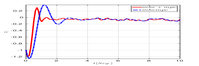
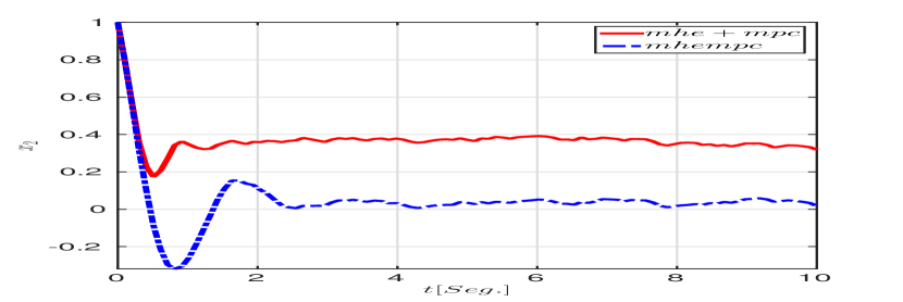
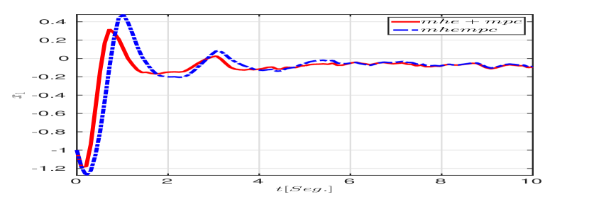
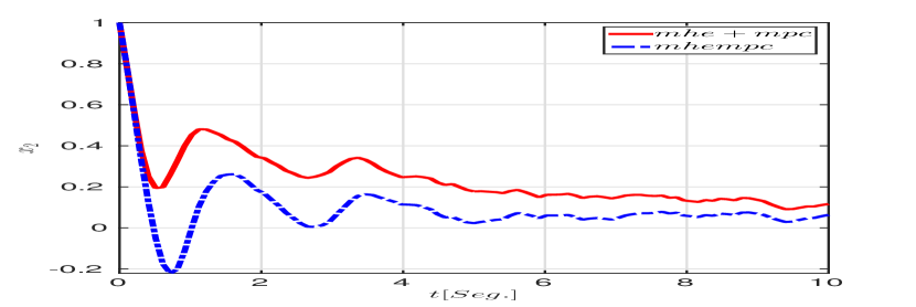
Figures 5 show the simulations resulting from two noise realizations for , and , respectively. They show that the simultaneous MHE–MPC manages to regulate both states and it achieves a better performance than the independent one. While Figures 5(a) and 5(c) show that independent MHE and MPC achieves a better performance than the simultaneous one for state , Figures 5(b) and 5(d) show how it fails to regulate state for short estimation horizons. Under this condition, has an offset that it is not compensated by the controller. Only large values of allow the independent MHE and MPC to regulate (Figure 5(d)). On the other hand, the simultaneous MHE–MPC regulates both states and it takes shorter times than the independent one to regulate both states.
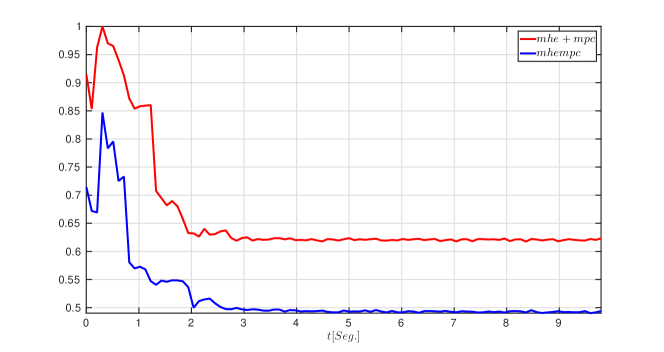 |
The computational burden of the simultaneous MHE–MPC is lower than the independent one, as can be seen in Figure 6. The execution times were averaged over trials. The lower time, in the beginning, is due to the backward window corresponding to the estimation has not achieved yet its full length.
5 Conclusions
We presented an output-feedback approach for nonlinear systems subject to bounded disturbances using MHE–MPC. The proposed approach combines the state estimation and control problems into a single optimization, which is solved at each sampling time. Theorem 1 states the necessary conditions to guaranty the feasibility and stability of the optimization problem, and therefore the boundedness of system states, as a function of the windows lengths and . This result requires the compatibility between the robust estimated and controllable sets (Assumption 1) and the existence of a relaxed closed–loop Lyapunov function for the disturbed system (Assumption 18). These conditions imply forward () and backward () horizons to find state estimates and control actions that are consistent with the system dynamics, constraints and disturbances. Future work may involve the design of the forward window with properties that allow the improvement of the estimation process and the design of an adaptive law to compute such that the estimation and control problems keep balanced and the overall system performance and numerical properties are improved.
References
- (1)
- Alessandri et al. (2005) Alessandri, A., Baglietto, M. & Battistelli, G. (2005), ‘Robust receding-horizon state estimation for uncertain discrete-time linear systems’, Systems & Control Letters 54(7), 627–643.
- Alessandri et al. (2008) Alessandri, A., Baglietto, M. & Battistelli, G. (2008), ‘Moving-horizon state estimation for nonlinear discrete-time systems: New stability results and approximation schemes’, Automatica 44(7), 1753–1765.
- Alessandri et al. (2012) Alessandri, A., Baglietto, M. & Battistelli, G. (2012), ‘Min-max moving-horizon estimation for uncertain discrete-time linear systems’, SIAM Journal on Control and Optimization 50(3), 1439–1465.
- Allan & Rawlings (2019) Allan, D. A. & Rawlings, J. B. (2019), A lyapunov-like function for full information estimation, in ‘2019 American Control Conference (ACC)’, IEEE, pp. 4497–4502.
- Åström (2012) Åström, K. J. (2012), Introduction to stochastic control theory, Courier Corporation.
- Bemporad et al. (2003) Bemporad, A., Borrelli, F. & Morari, M. (2003), ‘Min-max control of constrained uncertain discrete-time linear systems’, IEEE Transactions on automatic control 48(9), 1600–1606.
- Bemporad & Morari (1999) Bemporad, A. & Morari, M. (1999), Robust model predictive control: A survey, in ‘Robustness in identification and control’, Springer, pp. 207–226.
- Bensoussan (2004) Bensoussan, A. (2004), Stochastic control of partially observable systems, Cambridge University Press.
- Camacho & Alba (2004) Camacho, E. & Alba, B. (2004), ‘Model predictive control’.
- Chen & Allgöwer (1998) Chen, H. & Allgöwer, F. (1998), ‘A quasi-infinite horizon nonlinear model predictive control scheme with guaranteed stability’, Automatica 34(10), 1205–1217.
- Copp & Hespanha (2014) Copp, D. A. & Hespanha, J. P. (2014), Nonlinear output-feedback model predictive control with moving horizon estimation, in ‘53rd IEEE conference on decision and control’, IEEE, pp. 3511–3517.
- Copp & Hespanha (2016a) Copp, D. A. & Hespanha, J. P. (2016a), Conditions for saddle-point equilibria in output-feedback mpc with mhe, in ‘2016 American Control Conference (ACC)’, IEEE, pp. 13–19.
- Copp & Hespanha (2017) Copp, D. A. & Hespanha, J. P. (2017), ‘Simultaneous nonlinear model predictive control and state estimation’, Automatica 77, 143–154.
- Copp & Hespanha (2016b) Copp, D. & Hespanha, J. (2016b), Addressing adaptation and learning in the context of model predictive control with moving-horizon estimation, in ‘Control of Complex Systems’, Elsevier, pp. 187–209.
- Deniz et al. (2019) Deniz, N. N., Murillo, M. H., Sanchez, G., Genzelis, L. M. & Giovanini, L. (2019), ‘Robust stability of moving horizon estimation for nonlinear systems with bounded disturbances using adaptive arrival cost’, arXiv preprint arXiv:1906.01060 .
- Duncan & Varaiya (1971) Duncan, T. & Varaiya, P. (1971), ‘On the solutions of a stochastic control system’, SIAM Journal on Control 9(3), 354–371.
- Ellis et al. (2017) Ellis, M., Liu, J. & Christofides, P. D. (2017), State estimation and empc, in ‘Economic Model Predictive Control’, Springer, pp. 135–170.
- Findeisen et al. (2003) Findeisen, R., Imsland, L., Allgower, F. & Foss, B. A. (2003), ‘State and output feedback nonlinear model predictive control: An overview’, European journal of control 9(2-3), 190–206.
- Garcia-Tirado et al. (2016) Garcia-Tirado, J., Botero, H. & Angulo, F. (2016), ‘A new approach to state estimation for uncertain linear systems in a moving horizon estimation setting’, International Journal of Automation and Computing 13(6), 653–664.
- Georgiou & Lindquist (2013) Georgiou, T. T. & Lindquist, A. (2013), ‘The separation principle in stochastic control, redux’, IEEE Transactions on Automatic Control 58(10), 2481–2494.
- Grüne & Pannek (2011) Grüne, L. & Pannek, J. (2011), ‘Nonlinear model predictive control. communications and control engineering’, Springer. doi 10, 978–0.
- Ji et al. (2015) Ji, L., Rawlings, J. B., Hu, W., Wynn, A. & Diehl, M. (2015), ‘Robust stability of moving horizon estimation under bounded disturbances’, IEEE Transactions on Automatic Control 61(11), 3509–3514.
- Ji et al. (2016) Ji, L., Rawlings, J. B., Hu, W., Wynn, A. & Diehl, M. (2016), ‘Robust stability of moving horizon estimation under bounded disturbances’, IEEE Transactions on Automatic Control 61(11), 3509–3514.
- Kerrigan & Maciejowski (2000) Kerrigan, E. C. & Maciejowski, J. M. (2000), Invariant sets for constrained nonlinear discrete-time systems with application to feasibility in model predictive control, in ‘Proceedings of the 39th IEEE Conference on Decision and Control (Cat. No. 00CH37187)’, Vol. 5, IEEE, pp. 4951–4956.
- Magni et al. (2003) Magni, L., De Nicolao, G., Scattolini, R. & Allgöwer, F. (2003), ‘Robust model predictive control for nonlinear discrete-time systems’, International Journal of Robust and Nonlinear Control: IFAC-Affiliated Journal 13(3-4), 229–246.
- Magni et al. (2009) Magni, L., Raimondo, D. M. & Allgöwer, F. (2009), ‘Nonlinear model predictive control’, Lecture Notes in Control and Information Sciences (384).
- Mayne (2016) Mayne, D. (2016), ‘Robust and stochastic model predictive control: Are we going in the right direction?’, Annual Reviews in Control 41, 184–192.
- Mayne (2014) Mayne, D. Q. (2014), ‘Model predictive control: Recent developments and future promise’, Automatica 50(12), 2967–2986.
- Mayne et al. (2006) Mayne, D. Q., Raković, S., Findeisen, R. & Allgöwer, F. (2006), ‘Robust output feedback model predictive control of constrained linear systems’, Automatica 42(7), 1217–1222.
- Mayne et al. (2009) Mayne, D. Q., Raković, S., Findeisen, R. & Allgöwer, F. (2009), ‘Robust output feedback model predictive control of constrained linear systems: Time varying case’, Automatica 45(9), 2082–2087.
- Mayne et al. (2000) Mayne, D. Q., Rawlings, J. B., Rao, C. V. & Scokaert, P. O. (2000), ‘Constrained model predictive control: Stability and optimality’, Automatica 36(6), 789–814.
- Miettinen (2012) Miettinen, K. (2012), Nonlinear multiobjective optimization, Vol. 12, Springer Science & Business Media.
- Müller (2017) Müller, M. A. (2017), ‘Nonlinear moving horizon estimation in the presence of bounded disturbances’, Automatica 79, 306–314.
- Patwardhan et al. (2012) Patwardhan, S. C., Narasimhan, S., Jagadeesan, P., Gopaluni, B. & Shah, S. L. (2012), ‘Nonlinear bayesian state estimation: A review of recent developments’, Control Engineering Practice 20(10), 933–953.
- Pogromsky & Matveev (2015) Pogromsky, A. Y. & Matveev, A. S. (2015), ‘Stability analysis via averaging functions’, IEEE Transactions on Automatic Control 61(4), 1081–1086.
- Raimondo et al. (2009) Raimondo, D. M., Limon, D., Lazar, M., Magni, L. & ndez Camacho, E. F. (2009), ‘Min-max model predictive control of nonlinear systems: A unifying overview on stability’, European Journal of Control 15(1), 5–21.
- Rao et al. (2001) Rao, C. V., Rawlings, J. B. & Lee, J. H. (2001), ‘Constrained linear state estimation—a moving horizon approach’, Automatica 37(10), 1619–1628.
- Rao et al. (2003) Rao, C. V., Rawlings, J. B. & Mayne, D. Q. (2003), ‘Constrained state estimation for nonlinear discrete-time systems: Stability and moving horizon approximations’, IEEE transactions on automatic control 48(2), 246–258.
- Rawlings & Bakshi (2006) Rawlings, J. B. & Bakshi, B. R. (2006), ‘Particle filtering and moving horizon estimation’, Computers & chemical engineering 30(10-12), 1529–1541.
- Rawlings & Mayne (2009) Rawlings, J. B. & Mayne, D. Q. (2009), Model predictive control: Theory and design, Nob Hill Pub. Madison, Wisconsin.
- Rawlings et al. (2017) Rawlings, J. B., Mayne, D. Q. & Diehl, M. (2017), Model Predictive Control: Theory, Computation, and Design, Nob Hill Publishing.
- Roset et al. (2006) Roset, B., Lazar, M., Nijmeijer, H. & Heemels, W. (2006), Stabilizing output feedback nonlinear model predictive control: An extended observer approach, in ‘17th Symposium on Mathematical Theory for Networks and Systems. Kyoto, Japan’, Citeseer.
- Sánchez et al. (2017) Sánchez, G., Murillo, M. & Giovanini, L. (2017), ‘Adaptive arrival cost update for improving moving horizon estimation performance’, ISA transactions 68, 54–62.
- Schweppe (1973) Schweppe, F. C. (1973), Uncertain dynamic systems, Prentice Hall.
- Sontag & Wang (1995) Sontag, E. D. & Wang, Y. (1995), ‘On characterizations of the input-to-state stability property’, Systems & Control Letters 24(5), 351–359.
- Tuna et al. (2006) Tuna, S. E., Messina, M. J. & Teel, A. R. (2006), Shorter horizons for model predictive control, in ‘2006 American Control Conference’, IEEE, pp. 6–pp.
- Voelker et al. (2010) Voelker, A., Kouramas, K. & Pistikopoulos, E. N. (2010), ‘Unconstrained moving horizon estimation and simultaneous model predictive control by multi-parametric programming’.
- Voelker et al. (2013) Voelker, A., Kouramas, K. & Pistikopoulos, E. N. (2013), ‘Moving horizon estimation: Error dynamics and bounding error sets for robust control’, Automatica 49(4), 943–948.
- Zhang & Liu (2013) Zhang, J. & Liu, J. (2013), ‘Lyapunov-based mpc with robust moving horizon estimation and its triggered implementation’, AIChE Journal 59(11), 4273–4286.
Appendix A Proof Theorem 1
In the following we will analyse the stability of the simultaneous MHE–MPC algorithm by means of the difference in costs at two consecutive sampling time
| (41) |
Evaluating with the tail of the solution computed at time , with and , we obtain
| (42) |
Since and
| (43) |
then . Using inequality (18) and Assumption 5, can be rewritten as follows
| (44) |
for . Defining functions and as follows
| (45) |
the equation (44) can be written in a compact way
| (46) |
The term quantifies the improvements in the control cost (through the ratio between the cost-to-go and the control stage cost at time ) and the disturbance controllability (the ratio between the control stage costs and at time ).
The term quantifies the changes in the estimation cost by measuring the amount of information left behind the estimation window (the arrival–cost ). Since was computed within the control window (maximized), it tends to take larger values than which was computed within the estimation window (minimized). Therefore, when state estimation is precise (i.e., remains low), the term will tend to take positive values, whereas if a major correction is made on the initial condition (i.e., will take big values), the improvement in the estimated trajectory will lead a decreasing cost with sharper slope.
Since
| (47) |
which can be written in term of functions as follows (Deniz et al. 2019)
| (48) |
Restating (46) with , can be posed as
| (49) |
From the first term in the right hand side of (49), one can see that if
| (50) |
then, for large values of so that it becomes dominating in (49), the sequence of cost will present a contractive behaviour until reaches the value of . Therefore, we are looking for a control horizon large enough such that
| (51) |
Since by assumption 5, right hand side of inequality (51) will be positive. The problem consists now in to find a value of such that (51) be verified. In order to relate (51) with , let us note that
| (52) |
The term is upper bounded as (Tuna et al. 2006)
| (53) |
where is the term of the sequence from assumption 4 and . Then
| (54) |
If one choose the length of the control window with the following criterion
| (55) |
the following inequality holds
| (56) |