Analysis of the Relation between Quadratic Unconstrained Binary Optimization (QUBO) and the Spin Glass Ground-State Problem

Abstract

We analyze the transformation of QUBO from its conventional Boolean presentation into an equivalent spin glass problem with coupled $\pm 1$ spin variables exposed to a site-dependent external field. We find that in a widely used testbed for QUBO these fields tend to be rather large compared to the typical coupling and many spins in each optimal configuration simply align with the fields irrespective of their constraints. Thereby, the testbed instances tend to exhibit large redundancies - seemingly independent variables which contribute little to the hardness of the problem, however. We demonstrate various consequences of this insight, for QUBO solvers as well as for heuristics developed for finding spin glass ground states. To this end, we implement the Extremal Optimization (EO) heuristic, in a new adaptation for the QUBO problem. We also propose a novel way to assess the quality of heuristics for increasing problem sizes based on asymptotic scaling.

I Introduction

Quadratic unconstrained binary optimization (QUBO) is a versatile NP-hard combinatorial problem with applications in operations research Lü et al. (2010) and financial assets management, for example. It has recently been studied also as a benchmark challenge for the D-Wave quantum annealer McGeoch and Wang (2013) or for a new generation of classical optimizers based on GPU-technology Aramon et al. (2019). Cutting-edge classical algorithms for QUBO, developed in the engineering literature, are based on TABU search Wang et al. (2013); Glover et al. (2010); Lü et al. (2010); Boros et al. (2007); Palubeckis (2006) and a variety of other heuristics Kochenberger et al. (2014). From a statistical physics perspective, these developments are tantalizing for the fact that the generic formulation of QUBO appears to be identical to that of the Ising spin-glass Hamiltonian. While this connection has long be realized Barahona et al. (1988), it poses a conundrum that has not be commented on previously, and whose resolution could be of importance for both, the study of the low-energy structure of spin glasses as well as the understanding of its combinatorial hardness, for example, to assess the capabilities of the aforementioned solvers, classical and quantum.

Short of a real quantum computing solution, our only hope to find approximate solutions of reasonable quality for large-size instances of many NP-hard combinatorial optimization problems stems from the design of heuristic methods Hartmann and Rieger (2004); Hoos and Stützle (2004); Osman and Kelly (1996); Martello et al. (1999). From that perspective, it is somewhat surprising to find that seemingly equivalent instances of QUBO are routinely solved with well up to $N\approx 10^{4}$ variables Glover et al. (2010); Lü et al. (2010); Palubeckis (2006); Wang et al. (2013) while solvers for comparable spin glasses already struggle with instances of $N\approx 10^{3}$ variables to converge without incurring unacceptable systematic errors Hartmann (2001); Palassini and Young (1999); Pal (2006); Boettcher (2010a, 2005). Could adapting those highly developed QUBO solvers from the operations research literature provide a significant new inroad into investigations of spin glasses? What we find instead, unfortunately, is that there is an inherent weakness in the definition of the typical testbeds employed to assess QUBO solvers, which is revealed when these testbed instances are expressed as mean-field spin glasses. Exploiting this weakness, we apply a novel implementation of the Extremal Optimization (EO) heuristic Boettcher and Percus (2000, 2001); Hartmann and Rieger (2004); Middleton (2004) to the QUBO problem that performs on par with QUBO solvers for such large instances. In turn, we demonstrate that a naive application of a typical QUBO solver performs poorly for the spin glass. However, it would be of considerable physics interest to harness the power of TABU search and have experts in the design of QUBO solvers tune their implementations for spin glass problems for a fair comparison.

Besides of the caution against over-interpreting the significance of solving “large” instances, our study also produces a number of positive results. Our new implementation of EO not only serves as an alternative QUBO solver, but its design also provides insights that will advance the future exploration of the low-energy landscape of Ising spin glasses in the presence of external fields. Furthermore, we propose a powerful test for heuristic solvers that, in contrast with traditional testbed instances, unambiguously reveals the scalability of solvers asymptotically with problem size.

This paper is organized as follows: in Sec. II, we revisit the well-known relation between QUBO and spin glasses, with the added twist of a gauge transformation. In Sec. III, we adapt a sophisticated implementation of TABU search to study ground states of mean-field (Sherrington-Kirkpatrick) spin glasses. In Sec. IV, we employ EO to study the QUBO problem in a manner that incorporates well-known testbeds while also arguing for a novel way of quantifying the scalability of heuristics. In Sec. V, we conclude with an assessment of the state of the art for solving QUBO problems with heuristics and provide an outlook on future work.

II Relation Between Spin Glasses and QUBO

Disordered Ising spin systems in the mean-field limit have been investigated extensively as models of combinatorial optimization problems Mézard et al. (1987); Percus et al. (2006). Particularly simple are such models on (sparse) $\alpha$-regular random graphs (“Bethe-lattice”), where each vertex possesses a fixed number $\alpha$ of bonds to randomly selected other vertices Mézard and Parisi (2001); Boettcher (2003), or on a (dense) fully connected graph, referred to as the Sherrington-Kirkpatrick model (SK) Sherrington and Kirkpatrick (1975); Mézard et al. (1987); Boettcher (2005). Instances in an ensemble are formed via a matrix $J_{ij}$ of bonds between adjacent vertices $i$ and $j$, typically drawn randomly from a symmetric distribution such as ${\cal N}(0,1)$ (normal, Gaussian) or $\pm 1$ (bi-modal). (Accordingly, it is $J_{ii}\equiv 0$, as there are no “self-bonds”.) A dynamic variable $\sigma_{i}\in\{-1,+1\}$ (“spin”) is assigned to each vertex. Interconnecting loops of existing bonds lead to competing constraints and “frustration” Toulouse (1977), making optimal (minimal energy) spin configurations hard to find. In addition, we will allow for each spin to experience an external torque due to local magnetic fields $h_{i}$, which may also be drawn randomly or be of uniform fixed value. In the SK problem discussed here, we will merely consider the case of field-free instances ($h_{i}\equiv 0$). However, in the discussion of the relation between QUBO and SK, we will have to provide for the possibility of non-zero fields. Hence, as our cost function of this generalized problem, we endeavor to minimize the energy $H$ of the system,

$$H = -\sum_{i=1}^{N}\sum_{j=i+1}^{N}J_{ij}\sigma_{i}\sigma_{j}-\sum_{i=1}^{N}h_{i}\sigma_{i},$$ (1)

over the variables $\sigma_{i}$.

In turn, for QUBO we minimize the cost function

$$E=-\sum_{i=1}^{N}\sum_{j=1}^{N}q_{ij}x_{i}x_{j},$$ (2)

over a set of $N$ Boolean variables $x_{i}\in\left\{0,1\right\}$. Note that in this case it is $q_{ii}\not=0$, unlike for spin-glass couplings in Eq. (1). A generalized form of the QUBO cost with a term linear in the variables, similar to SK with an external field in Eq. (1), is not necessary, since we can use the identity $x_{i}\equiv x_{i}^{2}$, valid for $x_{i}\in\left\{0,1\right\}$, to write any linear terms as $cx_{i}=cx_{i}^{2}$ and add weights $c$ to that on the diagonal, $q_{ii}$. The test instances often considered for QUBO are created by choosing symmetric weights $q_{ij}$, drawn from a uniform (typically flat) distribution of zero mean, such as $-100<q_{ij}<100$ filling $N\times N$ matrices with 10-100% density Beasley ; Lü et al. (2010); Glover et al. (2010). (It seems that samples of sparse instances comparable to Bethe-lattices have not yet been discussed for QUBO.) In that literature, there is a distinct focus on specific testbeds of a few instances that are referenced for every new method applied to the problem, in an attempt to facilitate comparisons between the methods. Here, we merely consider a set of 10 such testbed instances from each of the sets “bqp1000” and “bqp2500”, of size $N=1000$ and 2500, respectively, to also allow for such a comparison. However, as we will see, significant insight, especially about the scaling with $N$ of each problem, can be gained by instead taking an ensemble perspective, i.e., we will make cost averages obtained over a larger number of instances taken at random from the ensemble at various sizes $N$.

Both problem statements, Eqs. (1-2), appear to be rather similar, including the symmetric distribution of weights and variables of a binary type, and one may wonder whether a detailed comparison between QUBO and SK as distinct optimization problems is warranted. Yet, the fact that spin glasses are defined for Ising variables, $\sigma_{i}\in\left\{\pm 1\right\}$, while QUBO has Boolean variables, $x_{i}\in\left\{0,1\right\}$, proves quite consequential.

II.1 Spin Glass as a QUBO Problem

For using a QUBO solver to optimize the SK spin glass problem in Sec. III, we have to rewrite the spin-glass cost function in Eq. (1) in terms of the Boolean variables a QUBO solver operates on. To that end, we assume given bonds $J_{ij}$ and fields $h_{i}$ and set $\sigma_{i}=2x_{i}-1$ to obtain

$$H=2E+C,$$ (3)

with $C=-\sum_{i=1}^{N}\sum_{j=i+1}^{N}J_{ij}+\sum_{i=1}^{N}h_{i}$ as some fixed constant for each instance. Now, $E$ takes on exactly the form of Eq. (2) but with weights

$$q_{ij} = \begin{cases}J_{ij},&i\not=j,\\ \\ h_{i}-\sum_{l=1}^{N}J_{il},&i=j.\end{cases}$$ (4)

Thus, by solving the QUBO problem for $E$ with these weights, we easily extract the spin glass ground state $H$ via Eq. (3). Note that although all $q_{ij}$ for $i\not=j$ are still simply random numbers drawn from a symmetric distribution, the diagonal elements $q_{ii}$ instead become extensive sums of such numbers, unless all $h_{i}\not=0$ and are specifically chosen as counterbalance. Such $q_{ii}$ are still symmetrically – but far more broadly – distributed (by a factor $\sim\sqrt{N}$) and always determined such that each row-sum and column-sum vanishes. Since $x_{i}^{2}\equiv x_{i}$, those diagonal elements are apparently equivalent to a linear term supplementing the QUBO cost-function, Eq. (2). However, the properties of such a term are quite different from the magnetic field term in Eq. (1), as we will discuss in Sec. IV.2.1.

II.2 QUBO Problem as a Spin Glass

Using a spin-glass solver to optimize the QUBO problem in Sec. IV, correspondingly, we take the QUBO weights $q_{ij}$ as given and rewrite the QUBO variables $x_{i}$ as spins $\sigma_{i}\in\left\{\pm 1\right\}$ via $x_{i}=\frac{1}{2}\left(1+\sigma_{i}\right)$. With that, in full analogy with Eq. (3), we find

$$E=\frac{1}{2}H-\frac{1}{2}C$$ (5)

with a Hamiltonian as given in Eq. (1) when using the bonds and fields as

$$h_{i} =\sum_{j=1}^{N}q_{ij},$$ (6)

$$J_{ij} =\begin{cases}q_{ij},&i\not=j,\\ \\ 0,&i=j.\end{cases}$$ (7)

Here, $C=\sum_{i=1}^{N}\sum_{j=i+1}^{N}q_{ij}+\sum_{i=1}^{N}q_{ii}$ again is an inert constant that is easily evaluated for each instance. Note that each single field $h_{i}$ itself becomes a symmetrically distributed random variable of width $\sim\sqrt{N}$, a sum over an entire row of the $q_{ij}$-matrix, if $q_{ij}$ is such a random variable of unit width. Such a strong biasing field, as we will argue in detail below, poses a serious problem for the design of truly hard QUBO instances. We will discuss in more detail how to find approximate ground states of such a spin-glass Hamiltonian with an external field in Sec. IV. However, given that, the cost for the QUBO problem follows simply from Eq. (5).

II.3 Gauge Transformation

While the existence of a relation between QUBO and spin glasses is not a novel observation Barahona et al. (1988); Kochenberger et al. (2014), the following consideration, albeit simple, allows for a pertinent insight into the nature of optimal configurations of QUBO that seems to have escaped prior notice. In general, a spin-glass Hamiltonian as in Eq. (1) retains all its spectral properties (here, in particular, its ground-state energy) under the transformation

$$\sigma_{i}\to\sigma_{i}^{\prime}=\xi_{i}\sigma_{i},\qquad\xi_{i}=\pm 1,$$ (8)

for all $i$. Then,

$$H\left(\left\{\sigma_{i}^{\prime}\right\}\right) = -\sum_{i}\sum_{j}\xi_{i}\xi_{j}J_{ij}\sigma_{i}\sigma_{j}-\sum_{i}\xi_{i}h_{i}\sigma_{i},$$

$$= -\sum_{i}\sum_{j}J_{ij}^{\prime}\sigma_{i}\sigma_{j}-\sum_{i}h_{i}^{\prime}\sigma_{i},$$

when we identify

$$J_{ij}^{\prime}=\xi_{i}\xi_{j}J_{ij},\qquad h_{i}^{\prime}=\xi_{i}h_{i},$$ (10)

Thus, the transformation in Eq. (8) leaves the spin-glass Hamiltonian invariant. We note that such an invariance does not exist for the (Boolean) QUBO problem, as the corresponding transformation $x_{i}\to x_{i}^{\prime}=1-x_{i}$ on only select sites $i$ modifies the QUBO Hamiltonian in Eq. (2).

Via Eq. (10), we are now free to “gauge” our spin variables in any form desirable. For our purposes, it is enlightening here to choose the set $\left\{\xi_{i}\right\}$ such that all external fields are non-negative, $h_{i}^{\prime}\geq 0$ for all $i$ in Eq. (10). We can easily obtain the solution of the original problem via $H(\left\{\xi_{i}\sigma_{i}\right\})=H^{\prime}(\left\{\sigma_{i}\right\})$, in particular, for the optimal configuration. It is now intuitive to ask: To what extend do spins in the optimal configuration align with their external field, irrespective of the mutual couplings $J_{ij}$? We will address that question in Sec. IV. First, we will explore how a QUBO solver fares in finding SK ground states.

III Using QUBO Solvers for SK

Here, we will apply a freely available QUBO solver, namely the Iterated Tabu Search (ITS) designed by G. Palubeckis in the implementation download from https://www.personalas.ktu.lt/~ginpalu/. In Ref. Palubeckis (2006), this implementation of ITS was used to reproduce the best-known results for various QUBO testbed instances (such as those discussed in Sec. IV) of up to $N=7000$ variables. Similar results were found with other implementations of Tabu-based QUBO solvers Kochenberger et al. (2014), and we assume the following observations to be generic for that class of solvers. We modify the ITS implementation only in so far as to input a large number of instances drawn from the SK-ensemble with bimodal bonds and to convert those into QUBO, as introduced in Sec. II.1. Experts in Tabu Search will note that no effort has been undertaken to tune the heuristic for the different ensemble, for which we have insufficient experience to accomplish. Thus, the following results are meant to serve as an illustration that a successful application to large QUBO instances does not imply the same for spin glasses.

This optimization problem of finding ground states of SK has been tackled previously using genetic algorithms Palassini (2008), hysteretic optimization Pal (2006); Gonçalves and Boettcher (2008), extremal optimization (EO) Boettcher (2005, 2010b), as well as various Metropolis methods Grest et al. (1986); Aspelmeier et al. (2008). In particular, in Refs. Boettcher (2005, 2010b), an asymptotic extrapolation was determined from finite-$N$ data with significant accuracy for the ensemble-averaged ground state energy,

$$\left\langle e_{0}\right\rangle_{N}=\left\langle e_{0}\right\rangle_{\infty}+\frac{A}{N^{\omega}}$$ (11)

with $\left\langle e_{0}\right\rangle_{\infty}=-0.76323(5)$, $A=0.70(1)$, and with $\omega=\frac{2}{3}$ conjectured to be exact. It provides a powerful reference – alternative to the results obtained from testbeds – for the quality of heuristic solvers, as shown in Fig. 1. There, we plot the results of our simulations where we have averaged over 1000 instances each for a range of sizes $N$. Those results are also listed in Tab. 1.

As we will compare below with data obtained for QUBO instances in dilute systems, we supplement this discussion further with a brief study of SK on a diluted graph. To be comparable with the QUBO instances, we consider SK in Eq. (1) with a symmetric bond matrix $J_{ij}$ whose off-diagonal elements are only to 10% non-zero (i.e., $\pm 1$). Again, we have no external fields. Those results are also listed in Tab. 1. These results, also shown in Fig. 1, are practically indistinguishable from those of the full SK. At around $N\approx 500$, ITS exhibits noticeable deviations from the apparent scaling. Novel to this case is the fact that we can arrive at this conclusion even though we have no knowledge a-priori about its asymptotic behavior, which further serves to demonstrate the value of such an extrapolation in assessing the ability of a heuristic. [The fact that the extrapolation based on our $\tau-$EO data according to Eq. (11) here requires an anomalous exponent of $\omega\approx 0.82$ is a novel result in itself and will be studied in more detail elsewhere.]

Table 1: Average ground state energy obtained for the SK spin glass, both at full bond-density (left columns) as well as at a 10% dilute bond-density (right columns), using the Iterated Tabu Search heuristic (ITS), as developed for QUBO in Ref. Palubeckis (2006), by sampling about 1000 instances at each size $N$, and applying default settings. In the dilute case, we also listed results for $\tau-$EO, which were generated here just for this comparison. These data points are also plotted in Fig. 1.

Full SK		SK at 10%
ITS		ITS		$\tau-$EO
$N$	$\left\langle e_{0}\right\rangle_{N}$	$N$	$\left\langle e_{0}\right\rangle_{N}$	$N$	$\left\langle e_{0}\right\rangle_{N}$
15	-0.644(2)	63	-0.2203(3)	63	-0.2204(1)
31	-0.692(1)	85	-0.2248(3)	85	-0.2248(1)
63	-0.7178(7)	127	-0.2291(2)	127	-0.2292(1)
127	-0.7358(5)	165	-0.2314(2)	165	-0.2314(1)
255	-0.7458(3)	255	-0.2342(1)	255	-0.2342(1)
511	-0.7519(2)	355	-0.2355(1)	355	-0.2357(1)
1023	-0.7520(1)	511	-0.2365(1)	511	-0.2371(2)
2047	-0.7491(1)	1023	-0.2366(1)	1023	-0.2389(3)

In either case, for small $N\lesssim 512$, the data obtained with Tabu Search tracks the prediction in Eq. (11) quite closely, thus demonstrating the consistency with the scaling in Eq. (11). However, systematic errors become increasingly apparent for larger system sizes. This raises the following conundrum: Why is a heuristic like ITS that routinely solves QUBO instances with 10 times as many variables failing to optimize SK instances beyond 500 variables, considering the rather similar formulations of both problems? A few immediately obvious explanations come to mind. For one, the ITS implementation has been tuned for a certain ensemble, as discussed in Sec. II, while the transformation of SK to QUBO provides a similar but not identical ensemble. (In fact, ITS specifically employs the strength of the diagonal $q_{ii}-$weights, which are very distinct in the SK problem, to initiate its restarts Palubeckis (2006).) Experts in Tabu-based heuristics could justifiably argue that with some small adjustments big improvements can be achieved. In fact, simply increasing the duration and the number of restarts in ITS leads to a decrease, albeit slowly, in the systematic error at larger $N$. Yet, the performance is never quite as impressive as the results obtained by Tabu solvers for the typical testbed instances of QUBO. We believe that the discrepancy is the sign of an inherent weakness in the design of the QUBO testbeds. This is made apparent by showing that heuristics trained on spin glasses in turn are easily adapted to solve much large samples of QUBO, as the following discussion suggests.

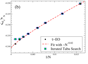
Figure 1: Extrapolation of the average ground-state energy approximation for the SK, either at full (top) or diluted bond-density (bottom), as obtained by Iterated Tabu Search Palubeckis (2006), see data listed in Tab. 1. For the full SK on top, the predicted scaling (red-dashed line) according to Eq. (11) was previously obtained from a fit to an extensive data set obtained with a different heuristic Boettcher (2010a). (For example, for $N\to\infty$ it extrapolates with high accuracy to the exactly known ground-state energy density of the SK model, $\left\langle e_{0}\right\rangle_{N=\infty}=\text{\textminus}0.763166\ldots$ Oppermann et al. (2007); Pankov (2006), marked by a blue arrow.) The dilute system on the bottom has not been studied before, so we have used $\tau-$EO to provide reference data (black circles), on which the predicted scaling is based via a fit (red-dashed line) to Eq. (11).

IV Using $\tau-$EO to Solve QUBO Problems

In this section, we proceed to apply heuristic methods developed for the approximation of spin-glass ground-states to the QUBO problem, specifically, $\tau-$EO Boettcher and Percus (2000, 2001); Hartmann and Rieger (2004). According to our prior experience, and in contrast to the preceding, somewhat naive application of the ITS heuristic, we are in a position to study this implementation in depth and develop a highly tuned heuristic. On one level, the equivalent spin-glass problem derived from QUBO, see Sec. II, raises additional challenges for EO, as the emergence of external fields add new, competing energy scales to reckon with. However, in the end, the comparison with the QUBO problem leads us to an understanding and, ultimately, to means to systematically incorporate these new scales into the search process. Moreover, an analysis of the solutions obtained for the QUBO problem as spin glass resolves the conundrum about the size discrepancy in the solvability of either problem mentioned in the previous section in physical terms.

IV.1 Extremal Optimization (EO) Heuristic

EO performs a local search Hoos and Stützle (2004) on an existing configuration of $N$ variables by changing preferentially those of poor local arrangement. For example, in case of the spin glass model in Eq. (1), but without an external field (i.e., $h_{i}\equiv 0$), one usually sets Boettcher and Percus (2001) $\lambda_{i}=\sigma_{i}\sum_{j}J_{i,j}\sigma_{j}$ to assess the local “fitness” of variable $\sigma_{i}$. Then, $H=-\sum_{i}\lambda_{i}$ represents the overall energy (or cost) to be minimized. EO simply ranks variables,

$$\lambda_{\Pi(1)}\leq\lambda_{\Pi(2)}\leq\ldots\leq\lambda_{\Pi(N)},$$ (12)

where $\Pi(k)=i$ is the index for the $k^{{\rm th}}$-ranked variable $\sigma_{i}$. Basic EO Boettcher and Percus (2000) always selects the lowest rank, $k=1$, for an update. Instead, $\tau-$EO selects the $k^{{\rm th}}$-ranked variable according to a scale-free probability distribution

$$P(k)\propto k^{-\tau}.$$ (13)

The selected variable is updated unconditionally, and its fitness and that of its neighboring variables are reevaluated. This update is repeated as long as desired, where the unconditional update ensures significant fluctuations, with sufficient incentive to return to near-optimal solutions due to selection against variables with poor fitness, for the right choice of $\tau$. Clearly, for finite $\tau$, this version of EO never “freezes” into a single configuration; it is able to return an extensive list Boettcher (2003); Boettcher and Percus (2004) of the best configurations visited (or simply their cost) “on the go” instead.

For $\tau=0$, the distribution in Eq. (13) becomes flat over the ranks and $\tau-$EO simply becomes a random walk through configuration space, for which poor search results are to be expected. Conversely, for $\tau\to\infty$, the process approaches a deterministic local search, only updating the lowest-ranked variable, $k=1$, and is likely to get trapped. However, for finite values of $\tau$ the choice of a scale-free distribution for $P(k)$ in Eq. (13) ensures that no rank $k$ gets excluded from further evolution, while maintaining a bias against variables with bad fitness. Fixing $\tau-1\sim 1/\ln(N)$ provides a simple, parameter-free strategy, activating avalanches of adaptation Boettcher and Grigni (2002).

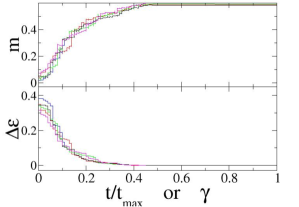
Figure 2: Plot of the evolution of EO in single runs for $\tau=1.3$ and $t_{max}=N^{3}/10$ updates, (top) for the magnetization and (bottom) the relative error $\Delta\epsilon$ with respect to the best-known value from Ref. Glover et al. (2010) for the instances of size $N=2500$ in the bqp testbed. Starting with a random assignment of spins at $\Delta\epsilon\approx 40\%$, better solutions are only obtained after the external fields are ramped up somewhat, according to Eq. (14). But note that the optimal solution is already found typically when the relative field strength reaches merely $\gamma\approx 50\%$. The fact that the magnetization of those optimal states reaches $m\approx 60\%$, i.e., up to 80% of spins simply align with their external field $h_{i}$, indicates a high degree of redundancy within those instances, see Fig. 3. A heuristic merely needs to sort out which 20% spins have to resist their external field.

IV.2 $\tau-$EO Implementation for QUBO

In light of previous applications to spin glasses, where fitness is defined via the local field exerted on each spin (see, for example, Sec. IV.1), it would seem straightforward to simply add the external field $h_{i}$ to the local field to obtain a definition of fitness as $\lambda_{i}=\sigma_{i}\left(h_{i}+\sum_{j}J_{i,j}\sigma_{j}\right)$, so that again $H=-\sum_{i}\lambda_{i}$, in accordance with Eq. (1). This canonical approach leads to a problem in which the heuristic is trying to satisfy two, in principle distinct, scales: that of the distribution of the bonds $J_{ij}$, and that of the distribution of the fields $h_{i}$. Since in the QUBO problem both scales derive from the one distribution of the weights $q_{ij}$, they are correlated in this case. Yet, in the optimization runs with $\tau-$EO on the testbed instances Boettcher (2015), for example, this definition of fitnesses $\lambda_{i}$ fails to provide reasonable results. Only when the external fields were slowly turned on, in those trials, via a ramp $\gamma$ that is linear in time,

$$\lambda_{i}=\sigma_{i}\left[\sum_{j=1}^{N}J_{ij}\sigma_{j}+\gamma(t)h_{i}\right],\qquad\gamma(t)=\frac{t}{t_{{\rm max}}},$$ (14)

the best-known results for that testbed were readily reproduced, albeit at significant overhead in CPU-time.

In Fig. 2, we plot the evolution of the error relative to that best-known result for each of the 10 instances of the testbed “bqp2500”, together with the corresponding magnetization. ( “Magnetization” here refers to the excess of spins aligned with their external fields $h_{i}$, whether those are positive or negative. Alternatively, it may refer to the actual magnetization, $m=\frac{1}{N}\sum_{i=1}^{N}\sigma_{i}$, due to the excess of spins with $\sigma_{i}=+1$ after applying the gauge transformation in Sec. II.3 that renders all fields $h_{i}^{\prime}>0$. Both formulations are equivalent!) At least, two aspects of those results are remarkable. For one, in each case, the best-found solution is found at least when those fields are “turned on” by 50%. Secondly, in that best-found solution there is a high degree of ordering imposed on the instance due to those external fields. We consider the importance of the latter observation first.

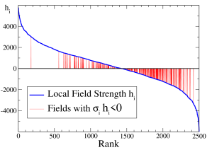
Figure 3: Analysis of the magnetization of the best-known solution to one of the bqp2500-instances from the QUBO testbed. Here, the rank-ordered list of $N=2500$ local fields $h_{i}$ defined in Eq. (6), corresponding to the row/column-sum of the weights $q_{ij}$, are plotted (blue line). Marked (by red vertical lines) are fields where the associated spin $\sigma_{i}$ in the configuration with the lowest energy is not aligned with $h_{i}$, i.e., when $\sigma_{i}h_{i}<0$. As the results for the magnetization in Fig. 2 suggest, only a small fraction ($\approx 20\%$) of variables do not align, in particular, most of those associated with the (absolute) highest fields (and, thus, largest contributions to the energy) are aligned (unmarked) with high probability.

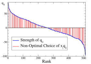
Figure 4: Analysis of the coercion of the diagonal element $q_{ii}$ in the QUBO matrix obtained from an SK spin-glass instance of size $N=511$ on the Boolean variables $x_{i}$ in the best-known solution. As in Fig. 3, the $q_{ii}$, obtained via Eq. (4), are plotted (in blue) in rank-order. Marked (by red vertical lines) are fields where the associated variable $x_{i}$ in the configuration with the lowest cost is not aligned to render $x_{i}q_{ii}$ optimal, i.e., when $x_{i}=0$ although $q_{ii}>0$ or $x_{i}=1$ while $q_{ii}<0$ . Unlike the local fields $h_{i}$ in Fig. 3, the strength of $q_{ii}$ here provides no distinguishable coersive force of the $x_{i}$.

IV.2.1 Magnetization of QUBO Instances:

Representing each testbed instance of QUBO as a spin glass, following Sec. II.2, we actually find that the magnetization reaches $\approx 60\%$, i.e., the alignment of the variables $\sigma_{i}$ with their external fields is to 80% a predictor of the optimal arrangement within the lowest-energy solution. Thus, irrespective of the mutual constraints spins impose on each other through the bonds $J_{ij}$, in many cases those constraints are simply overwritten by the torque exerted by the external fields $h_{i}$ alone. Clearly, a larger local field imposes a larger torque that is more likely coercive than a smaller one, as Fig. 3 illustrates. In fact, we find that a simple $O(N)$ “greedy alignment” algorithm that aligns spins sequentially, selected based on having the largest remaining local field (consisting of the torque exerted by the external field and those of any previously assigned spins), typically reaches a cost that is within 3% of the best-known solutions (see Fig. 6). Still, it likely remains an NP-hard task to sort out which 20% of the fields are to be disobeyed, although for each $N$ this is a problem of much reduced complexity compared to the corresponding SK ground state problem with all $h_{i}\equiv 0$, hence, explaining the discrepancy in “hardness” between QUBO and SK.

It is instructive to consider the – seemingly – equivalent representation of an SK-instance (without external field) as a QUBO problem. As mentioned in Sec. II.1, such a conversion produces a linear term in the QUBO cost-function of similar appearance to the magnetic field above. In particular, its strength, given by $q_{ii}$ in Eq. (4), appears to be as extensive as we found for the $h_{i}$. However, the coupling of each variable $x_{i}$ to $q_{ii}$ is somewhat arbitrary and, hence, fails to coerce $x_{i}$ in a significant manner, as is demonstrated in Fig. 4. To show this, we employ the freedom to gauge the SK-instance in question, following Sec. II.3, leaving open the choice for the entire set of gauge-parameters $\left\{\xi_{i}\right\}$. In the absence of an external field, Eq. (4) then yields:

$$q_{ii}=-\sum_{l=1}^{N}J_{il}\xi_{i}\xi_{l}.$$ (15)

Alas, different choices of $\xi_{i}=\pm 1$ create quite arbitrary linear couplings $q_{ii}$ for each individual $x_{i}$ (although overall the hardness of the problem is not affected)! In contrast, no such invariance exists for QUBO and, thus, the linear terms $h_{i}$ emerging in its conversion into a spin-glass problem are unique and render the coercive force on their coupled variable $\sigma_{i}$ consequential, see Fig. 3.

IV.2.2 Optimization of the EO-Implementation:

We now return to the earlier observation about $\tau-$EO saturating the best-known results in the testbed when the ramped fields in Eq. (14) reach 50% with striking consistency. As it turns out, this observation pins down an arbitrary choice in the design of EO that allows us to implement a more efficient version of $\tau-$EO. This choice in the definition of fitness attributed to individual variables has been discussed previously in Ref. Hartmann and Rieger (2004). It is here where the interpretation of spin glasses as a QUBO problem has its most significant impact. Unlike for a spin glass, where the combined local field offers itself as the canonical fitness for each spin, in QUBO we would naturally construct a fitness as follows instead: By assigning a variable $x_{i}$, its instantaneous contribution to the cost of $r_{i}=\sum_{j=1}^{N}q_{ij}x_{j}$ is either suppressed ($x_{i}=0$) or added ($x_{i}=1$), hence, the fitness $\lambda_{i}$ should be $r_{i}$ if $x_{i}=1$ or $-r_{i}$ if $x_{i}=0$, penalizing the un-actualized potential when $r_{i}>0$ but $x_{i}=0$. Thus, for QUBO the apparent choice for fitness can be summarized as

$$\lambda_{i}=\sigma_{i}\sum_{j=1}^{N}q_{ij}x_{j}.$$ (16)

Note that in this case, $\sum_{i}\lambda_{i}$ itself does not add up to the actual cost of an instance, $E$ or $H$, which is not a necessity, as is discussed in Ref. Hartmann and Rieger (2004). Amazingly, using the definitions in Sec. II, for the spin glass this translates into

$$\lambda_{i}=\sigma_{i}\left[\sum_{j=1}^{N}J_{ij}\sigma_{j}+\frac{1}{2}h_{i}\right],$$ (17)

i.e., favoring a fixed value of $\gamma=50\%$. This result is indeed borne out with a more systematic study at various fixed values of $\gamma$, as shown in Fig. 5. Accordingly, we will use this more effective version of $\tau-$EO in the following, with $\tau=1.3$ and $t_{max}=N^{3}/100$, and fitnesses as defined in Eq. (17), to study the QUBO problem as a spin glass. As such, $\tau-$EO has a complexity of $O\left(N^{3}\ln N\right)$, where the logarithmic dependence is due to dynamic sorting of fitnesses, as introduced in Ref. Boettcher (2005).

Figure 5: Study of the $\gamma-$dependence of the error $\epsilon$ produced by $\tau-$EO relative to the best-known results, averaged over the two QUBO gqp testbeds with $N=1000$ and $N=2500$, when using the fitnesses $\lambda_{i}=\sigma_{i}\left[\sum_{j=1}^{N}J_{ij}\sigma_{j}+\gamma h_{i}\right]$ with fixed $\gamma$ during a run, as generalization of Eq. (17). For $\tau-$EO, as described in Sec. IV.1, we set $\tau=1.3$ and $t_{max}=N^{3}/100$. The results clearly indicate $\gamma=50\%$ as an especially useful case, as implemented in Eq. (17).

Table 2: Results from applying $\tau-$EO to the QUBO ensemble defined in Sec. II, with $q_{ij}$ drawn randomly from a flat distribution over the integers on $\left[-100\ldots+100\right]$ at 10% filling. Listed are the system sizes $N$ considered, the number of instances $I$ simulated from the ensemble, the measured ground-state energy density $\left\langle e_{0}\right\rangle_{N}=H/N^{\frac{3}{2}}$ according to Eq. (1), and the corresponding approximation obtained with the greedy alignment algorithm. Note that the result for $N=1000$ and $N=2500$ specifically refer only to the gap testbeds (underlined). This data is plotted as an extrapolation plot in Fig. 6.

$N$	$I$	$\left\langle e_{0}\right\rangle_{N}$	Greedy
31	$10^{5}$	-9.67(1)	-9.46(1)
44	$10^{5}$	-10.074(5)	-9.81(1)
63	$10^{5}$	-10.318(5)	-10.036(5)
80	$10^{5}$	-10.426(4)	-10.125(4)
100	$10^{5}$	-10.501(4)	-10.190(5)
127	$10^{5}$	-10.564(3)	-10.245(3)
160	$2\,10^{4}$	-10.611(7)	-10.298(7)
255	$10^{4}$	-10.68(1)	-10.34(1)
511	$10^{4}$	-10.750(5)	-10.404(4)
1000	10	-11.4(1)	-11.1(1)
1023	$4\,10^{3}$	-10.776(6)	-10.44(1)
2500	10	-11.84(7)	-11.45(7)
4095	600	-10.79(1)	-10.48(2)

Figure 6: Extrapolation of the average optimal cost approximation for the QUBO problem as obtained by $\tau-$EO. All data displayed here can also be found in Tab. 2. We can fit the EO-data (black circles) for sufficiently small $N$ (which is more likely exact!), but $N\gtrsim 50$ to be asymptotic, to obtain a scaling prediction (red-dashed line) for all large $N$. A deviation from that scaling, which would signal the onset of systematic errors in the heuristic (as seen in Fig. 1), is not apparent here for the data up to $N=4095$. Shown are also the corresponding data for the greedy alignment algorithm mentioned in the text (blue squares), which remains systematically 3% above the optimal results for all $N$, another indication that the EO-data maintains its systematic accuracy. Strikingly, the averages for the best-found solutions for both testbeds, gqp1000 and gqp2500, are uncharacteristically low and far from their expected ensemble average (red-dashed line), but so are their greedy approximations (not shown here, but see Tab. 2), which are again 3% higher, yet, much below the ensemble. It seems likely that those gap testbed instances, originating in 1996 from Ref. Beasley (1996), were generated with a poor random number generator.

IV.3 Ensemble Results for the QUBO Problem

Based on the implementation of $\tau-$EO described in the previous section, we have run extensive simulations for the QUBO problem, similar to those we have employed previously for SK Boettcher (2005, 2010a). And in analogy with those, we propose here to evaluate the capabilities of the implementation using an extrapolation plot of the ensemble results, as also shown in Fig. 1. The results validate our expectation that QUBO problems in this ensemble can be solved to much larger sizes than the corresponding SK spin glass.

In Tab. 2, we summarize the results of the simulations for the range of instance sizes from $N=31,\ldots,4095$. For each size, we have selected a sufficiently large number of instances from the ensemble to be able to keep the statistical errors small and relatively comparable in magnitude. From SK, it is well-known that, if the matrix elements are drawn from a distribution of fixed width, scale-invariant (intensive) costs are obtained when $H$ is rescaled by a factor of $N^{\frac{3}{2}}$ Mézard et al. (1987), thus, we define $\left\langle e_{0}\right\rangle_{N}=H/N^{\frac{3}{2}}$, in accordance with Eq. (11). Listed are also the corresponding results for the described $O(N)$ Greedy Alignment algorithm, which turn out to be consistently 3% above the best EO predictions, another sign of their systematic quality.

This data is also plotted in Fig. 6, in extrapolated form, which should yield an asymptotically linear graph, according to Eq. (11), if we choose $N^{-\omega}$ with the correct value of $\omega$ as our $x-$axis. Such a linear extrapolation is achieved here for $\omega=1$, suggesting that finite-size corrections in QUBO diminish much faster than for SK, where corrections are conjectured to decay only as $N^{-\frac{2}{3}}$, i.e., $\omega=\frac{2}{3}$ Boettcher (2005); Billoire (2006); Aspelmeier et al. (2008), as shown in Fig. 1. Weaker corrections provide more evidence for the relative simplicity of approximating QUBO. As for the SK data in Refs. Boettcher (2005, 2010a), this data is also readily fitted asymptotically (for $N$ small enough that there a few systematic errors but large enough, here $N>44$, to ignore finite-size corrections) with the linear form provided by Eq. (11). Note that the specific values obtained for this fit, $\left\langle e_{0}\right\rangle_{\infty}=-10.8(1)$ and $A=30(1)$, are not of any significance by themselves. All we care about is a deviation from that line for large $N$ as a likely sign of a systematic breakdown in the heuristic we care to assess. Up to the sizes accessible with this implementation within reasonable CPU time, EO does not show any significant systematic error, as discussed in Fig. 7.

As a curious side-note, we observe that the 10 instances from the gap testbeds of sizes $N=1000$ and $N=2500$ (also listed in Tab. 2 and plotted as red dots in Fig. 6) apparently are highly atypical for the ensemble they were supposedly drawn from, with much lower average costs. This does not signal a shortcoming of EO, as all averages were obtained uniformly with the same implementation, and the greedy results are equally untypical but remain 3% above the best-found costs. We can only speculate about the origin of this effect, but it seems likely that a poor random number generator was used to make the testbed.

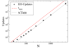
Figure 7: Measure of the computational cost for the $\tau-$EO implementation in terms of the average number of update steps needed to first encounter the best-found solutions listed in Tab. 2 as a function of instance size $N$. The cubic line (dotted) of $N^{3}/400$ is merely included to guide the eye. The approach of the measured updates suggest that EO typically finds its best solution within a quarter of the allotted number of updates, $t_{{\rm max}}=N^{3}/100$ (red-dashed line). Since the actual computational complexity for an NP-hard problem such as QUBO is expected to rise exponentially in size, we would expect EO to eventually exhibit systematic errors. However, up to this size, there is no sign of upward pressure on the total runtime.

V Conclusions

In our discussion, we have analyzed the relation between the SK spin glass ground-state problem and the classical NP-hard combinatorial problem of QUBO. We have argued that a widely used form of the QUBO problem, with weights drawn from a symmetric distribution of finite width, leads to rather simple testbeds with a high degree of redundancy. Those instances correspond to a spin glass problem where a large fraction of spins are independently determined by a large biasing field. As Eq. (6) shows, those biasing fields can only be avoided when in the QUBO problem the sum of the weights in each row (or column) vanishes, or at least grows less that $O(\sqrt{N})$ for increasing problem size $N$. We will explore more systematic approaches to generate matrices $Q$ that have random entries but are constraint to vanishing row-sums elsewhere. Since such problems have recently been used to assess the quality of dedicated quantum annealers McGeoch and Wang (2013) such as D-Wave, which claims advantages due to quantum effects, a careful analysis of actual hardness of classical problems is timely. In terms of the physical description of the QUBO problem as a Ising spin glass, we find that a large fraction of variables in those instances are trivially coerced by large external fields. The impact of this redundancy is illustrated first by applying a standard QUBO solver that provides good results for large QUBO instances but in turn fails for much smaller and seemingly similar SK instances. We then proposed an implementation of $\tau-$EO, previously well-trained on the SK problem, and show that it can solve comparatively much larger instances of the QUBO problem. Along the way, we have shown that a systematic, ensemble-based study to test the capabilities of heuristics via an extrapolation plot provides a self-contained and quite stringent measure of their performance for large $N$, superior to any ad-hoc assembly of testbeds.

In the future, we will explore whether the definition of fitness used in Eq. (17) for spin glasses in an external field, which our calculations show to remain valid when the external field is varied independently (unlike for the SK obtained from QUBO here), will allow to apply $\tau-$EO also to interesting ground state problems of spin glasses in such fields. A number of questions about the low-temperature glassy state of spin glasses are connected with its stability under coercion with external fields de Almeida and Thouless (1978); Jörg et al. (2008); Larson et al. (2013); Zintchenko et al. (2015).

References

- Lü et al. (2010) Z. Lü, F. S. Glover, and J.-K. Hao, European Journal of Operational Research 207, 1254 (2010).
- McGeoch and Wang (2013) C. C. McGeoch and C. Wang, in Proceedings of the ACM International Conference on Computing Frontiers, CF ’13 (ACM, New York, NY, USA, 2013) pp. 23:1–23:11.
- Aramon et al. (2019) M. Aramon, G. Rosenberg, E. Valiante, T. Miyazawa, H. Tamura, and H. G. Katzgraber, Frontiers in Physics 7 (2019), 10.3389/fphy.2019.00048.
- Wang et al. (2013) Y. Wang, Z. Lü, F. Glover, and J.-K. Hao, Computers & Operations Research 40, 3100 (2013).
- Glover et al. (2010) F. S. Glover, Z. Lü, and J.-K. Hao, 4OR - Q J Oper Res 8, 239 (2010).
- Boros et al. (2007) E. Boros, P. L. Hammer, and G. Tavares, J. Heuristics 13, 99 (2007).
- Palubeckis (2006) G. Palubeckis, Informatica 17, 279 (2006).
- Kochenberger et al. (2014) G. Kochenberger, J.-K. Hao, F. Glover, M. Lewis, Z. Lü, H. Wang, and Y. Wang, Journal of Combinatorial Optimization 28, 58 (2014).
- Barahona et al. (1988) F. Barahona, M. Grötschel, M. Jünger, and G. Reinelt, Oper. Res. 36, 493 (1988).
- Hartmann and Rieger (2004) A. Hartmann and H. Rieger, eds., New Optimization Algorithms in Physics (Wiley-VCH, Berlin, 2004).
- Hoos and Stützle (2004) H. H. Hoos and T. Stützle, Stochastic Local Search: Foundations and Applications (Morgan Kaufmann, San Francisco, 2004).
- Osman and Kelly (1996) I. H. Osman and J. P. Kelly, eds., Meta-Heuristics: Theory and Application (Kluwer, Boston, 1996).
- Martello et al. (1999) S. Martello, I. Osman, C. Roucairol, and S. Voss, eds., Meta-Heuristics: Advances and Trends in Local Search Paradigms for Optimization (Kluwer, Boston, 1999).
- Hartmann (2001) A. K. Hartmann, Phys. Rev. E 63 (2001).
- Palassini and Young (1999) M. Palassini and A. P. Young, Phys. Rev. Lett. 83, 5126 (1999).
- Pal (2006) K. F. Pal, Physica A 367, 261 (2006).
- Boettcher (2010a) S. Boettcher, J. Stat. Mech , P07002 (2010a).
- Boettcher (2005) S. Boettcher, Eur. Phys. J. B 46, 501 (2005).
- Boettcher and Percus (2000) S. Boettcher and A. G. Percus, Artificial Intelligence 119, 275 (2000).
- Boettcher and Percus (2001) S. Boettcher and A. G. Percus, Phys. Rev. Lett. 86, 5211 (2001).
- Middleton (2004) A. A. Middleton, Phys. Rev. E 69, 055701(R) (2004).
- Mézard et al. (1987) M. Mézard, G. Parisi, and M. A. Virasoro, Spin glass theory and beyond (World Scientific, Singapore, 1987).
- Percus et al. (2006) A. Percus, G. Istrate, and C. Moore, Computational Complexity and Statistical Physics (Oxford University Press, New York, 2006).
- Mézard and Parisi (2001) M. Mézard and G. Parisi, Eur. Phys. J. B 20, 217 (2001).
- Boettcher (2003) S. Boettcher, Euro. Phys. J. B 31, 29 (2003).
- Sherrington and Kirkpatrick (1975) D. Sherrington and S. Kirkpatrick, Phys. Rev. Lett. 35, 1792 (1975).
- Toulouse (1977) G. Toulouse, Communication on Physics 2, 115 (1977).
- Note (1) In the operations research literature, QUBO is usually defined as a maximization problem for without the sign; the conversion is trivial.
- (29) J. E. Beasley, “Heuristic algorithms for the unconstrained binary quadratic programming problem,” Tech. Rep., Management School, Imperial College (1998).
- Palassini (2008) M. Palassini, J. Stat. Mech. , P10005 (2008).
- Gonçalves and Boettcher (2008) B. Gonçalves and S. Boettcher, J. Stat. Mech. , P01003 (2008).
- Boettcher (2010b) S. Boettcher, Euro. Phys. J. B 74, 363 (2010b).
- Grest et al. (1986) G. S. Grest, C. M. Soukoulis, and K. Levin, Phys. Rev. Lett. 56, 1148 (1986).
- Aspelmeier et al. (2008) T. Aspelmeier, A. Billoire, E. Marinari, and M. A. Moore, Journal of Physics A: Mathematical and Theoretical 41, 324008 (21pp) (2008).
- Oppermann et al. (2007) R. Oppermann, M. J. Schmidt, and D. Sherrington, Phys. Rev. Lett. 98, 127201 (2007).
- Pankov (2006) S. Pankov, Phys. Rev. Lett. 96, 197204 (2006).
- Boettcher and Percus (2004) S. Boettcher and A. G. Percus, Phys. Rev. E 69, 066703 (2004).
- Boettcher and Grigni (2002) S. Boettcher and M. Grigni, J. Phys. A: Math. Gen. 35, 1109 (2002).
- Boettcher (2015) S. Boettcher, Physics Procedia 68, 16 (2015).
- Note (2) We thank the referee for insisting on this consideration.
- Beasley (1996) J. Beasley, Journal of Global Optimization 8, 429 (1996).
- Billoire (2006) A. Billoire, Phys. Rev. B 73, 132201 (2006).
- de Almeida and Thouless (1978) J. de Almeida and D. Thouless, J. Phys. A 11, 983 (1978).
- Jörg et al. (2008) T. Jörg, H. G. Katzgraber, and F. Krzakala, Physical Review Letters 100 (2008), 10.1103/physrevlett.100.197202.
- Larson et al. (2013) D. Larson, H. G. Katzgraber, M. A. Moore, and A. P. Young, Physical Review B 87 (2013), 10.1103/physrevb.87.024414.
- Zintchenko et al. (2015) I. Zintchenko, M. B. Hastings, and M. Troyer, Phys. Rev. B 91, 024201 (2015).