Hierarchical Colorings of Cographs

Abstract

Cographs are exactly hereditarily well-colored graphs, i.e., the graphs for which a greedy coloring of every induced subgraph uses only the minimally necessary number of colors $\chi(G)$. In recent work on reciprocal best match graphs so-called hierarchically coloring play an important role. Here we show that greedy colorings are a special case of hierarchical coloring, which also require no more than $\chi(G)$ colors.

Keywords: graph colorings: Grundy number; cographs; phylogenetic combinatorics

1 Introduction and Preliminaries

Let $G=(V,E)$ be an undirected graph. A (proper vertex) coloring of $G$ is a surjective function $\sigma:V\to S$ such that $xy\in E$ implies $\sigma(x)\neq\sigma(y)$. The minimum number $|S|$ of colors such that there is a coloring of $G$ is known as the chromatic number $\chi(G)$. A greedy coloring of $G$ is obtained by ordering the set of colors and coloring the vertices of $G$ in a random order with the first available color. The Grundy number $\gamma(G)$ is the maximum number of colors required in a greedy coloring of $G$ [2]. Obviously $\gamma(G)\geq\chi(G)$. Determining $\chi(G)$ [7] and $\gamma(G)$ [12] are NP-complete problems. A graph $G$ is called well-colored if $\chi(G)=\gamma(G)$ [12]. It is hereditarily well-colored if every induced subgraph is well-colored.

Definition 1.1 ([3]).

A graph $G$ is a cograph if $G=K_{1}$, $G$ is the disjoint union $G=\operatorname{\mathop{\vphantom{\bigcup}\mathchoice{\leavevmode\vtop{\halign{\hfil$\m@th\displaystyle#$\hfil\cr\bigcup\cr\cdot\crcr}}}{\leavevmode\vtop{\halign{\hfil$\m@th\textstyle#$\hfil\cr\bigcup\cr\cdot\crcr}}}{\leavevmode\vtop{\halign{\hfil$\m@th\scriptstyle#$\hfil\cr\bigcup\cr\cdot\crcr}}}{\leavevmode\vtop{\halign{\hfil$\m@th\scriptscriptstyle#$\hfil\cr\bigcup\cr\cdot\crcr}}}}\displaylimits}_{i}G_{i}$ of cographs $G_{i}$, or $G$ is a join $G=\mathop{\vphantom{\sum}\mathchoice{\vbox{\hbox{\leavevmode\resizebox{9.00005pt}{}{$\triangledown$}}}}{\vbox{\hbox{\leavevmode\resizebox{10.00012pt}{}{$\triangledown$}}}}{\vbox{\hbox{\leavevmode\resizebox{7.00009pt}{}{$\triangledown$}}}}{\vbox{\hbox{\leavevmode\resizebox{5.00006pt}{}{$\triangledown$}}}}}\slimits@_{i}G_{i}$ of cographs $G_{i}$.

This recursive construction induces a rooted tree $T$, whose leaves are individual vertices corresponding to a $K_{1}$ and whose interior vertices correspond to the union and join operations. We write $L(T)$ for the leaf set and $V^{0}(T)$ for the set of inner vertices of $T$. The set of children of $u$ is denoted by $\mathsf{child}(u)$. For edges $e=uv$ in $T$ we adopt the convention that $v$ is a child of $u$. We define a labeling function $t:V^{0}(T)\rightarrow\{0,1\}$, where an interior vertex $u$ of $T$ is labeled $t(u)=0$ if it is associated with a disjoint union, and $t(u)=1$ for joins. The set $L(T(u))$ denotes the leaves of $T$ that are descendants of $u$. To simplify the notation we will write $G(u):=G[L(T(u))]$ for the subgraph of $G$ induced by the vertices in $L(T(u))$. Note that $G(u)$ is the graph consisting of the single vertex $u$ if $u$ is a leaf of $T$.

Given a cograph $G$, there is a unique discriminating cotree in which adjacent operations are distinct, i.e., $t(u)\neq t(v)$ for all interior edges $uv\in E(T)$. It is possible to refine the discriminating cotree by subdiving a disjoint union or join into multiple disjoint unions or joins, respectively [1, 3]. It is well known that every induced subgraph of a cograph is again a cograph. A graph is a cograph if and only if it does not contain a path $P_{4}$ on four vertices as an induced subgraph [3]. The cographs are also exactly the hereditarily well-colored graphs [2]. The chromatic number of a cograph $G$ can be computed recursively, as observed in [3, Tab.1]. Starting from $\chi(K_{1})=1$ as base case we have

$$\begin{split}\chi(G)&=\chi\left(\operatorname{\mathop{\vphantom{\bigcup}\mathchoice{\leavevmode\vtop{\halign{\hfil$\m@th\displaystyle#$\hfil\cr\bigcup\cr\cdot\crcr}}}{\leavevmode\vtop{\halign{\hfil$\m@th\textstyle#$\hfil\cr\bigcup\cr\cdot\crcr}}}{\leavevmode\vtop{\halign{\hfil$\m@th\scriptstyle#$\hfil\cr\bigcup\cr\cdot\crcr}}}{\leavevmode\vtop{\halign{\hfil$\m@th\scriptscriptstyle#$\hfil\cr\bigcup\cr\cdot\crcr}}}}\displaylimits}_{i}G_{i}\right)=\max_{i}\chi(G_{i})\textrm{ or }\\ \chi(G)&=\chi\left(\mathop{\vphantom{\sum}\mathchoice{\vbox{\hbox{\leavevmode\resizebox{9.00005pt}{}{$\triangledown$}}}}{\vbox{\hbox{\leavevmode\resizebox{10.00012pt}{}{$\triangledown$}}}}{\vbox{\hbox{\leavevmode\resizebox{7.00009pt}{}{$\triangledown$}}}}{\vbox{\hbox{\leavevmode\resizebox{5.00006pt}{}{$\triangledown$}}}}}\slimits@_{i}G_{i}\right)=\sum_{i}\chi(G_{i})\end{split}$$ (1)

Hierarchically colored cograph (hc-cographs) were introduced in [5] as the undirected colored graphs recursively defined by

(K1)

$(G,\sigma)=(K_{1},\sigma)$, i.e., a colored vertex, or

(K2)

$(G,\sigma)=(H_{1},\sigma_{H_{1}})\operatorname{\triangledown}(H_{2},\sigma_{H_{2}})$ and $\sigma(V(H_{1}))\cap\sigma(V(H_{2}))=\emptyset$, or

(K3)

$(G,\sigma)=(H_{1},\sigma_{H_{1}})\mathbin{\mathchoice{\leavevmode\vtop{\halign{\hfil$\m@th\displaystyle#$\hfil\cr\cup\cr\cdot\crcr}}}{\leavevmode\vtop{\halign{\hfil$\m@th\textstyle#$\hfil\cr\cup\cr\cdot\crcr}}}{\leavevmode\vtop{\halign{\hfil$\m@th\scriptstyle#$\hfil\cr\cup\cr\cdot\crcr}}}{\leavevmode\vtop{\halign{\hfil$\m@th\scriptscriptstyle#$\hfil\cr\cup\cr\cdot\crcr}}}}(H_{2},\sigma_{H_{2}})$ and $\sigma(V(H_{1}))\cap\sigma(V(H_{2}))\in\{\sigma(V(H_{1})),\sigma(V(H_{2}))\}$,

where $\sigma(x)=\sigma_{H_{i}}(x)$ for every $x\in V(H_{i})$, $i\in\{1,2\}$ and $(H_{1},\sigma_{H_{1}})$ and $(H_{2},\sigma_{H_{2}})$ are hc-cographs.

This recursive construction of an hc-cograph $G$ implies a binary cotree $(T,t)$. Its inner vertices can be associated with the intermediate graphs in the construction. We say that $\sigma$ is an hc-coloring w.r.t. $(T,t)$.

Obviously, the graph $G$ underlying an hc-cograph is a cograph.

Definition 1.2.

Let $G=(V,E)$ be a cograph. A coloring $\sigma:V\to S$ of $G$ is an hc-coloring of $G$ if there is binary cotree $(T,t)$ of $G$ such that $(G,\sigma)$ is hc-cograph w.r.t. $(T,t)$.

This contribution aims to investigate the properties of hc-colorings and their relationships with other types of cograph colorings.

2 Existence of hc-Colorings

As noticed in [5], a coloring $\sigma$ of a cograph $G$ may be an hc-coloring w.r.t. some cotree $(T,t)$ but not w.r.t. to another cotree $(T^{\prime},t^{\prime})$ that yields the same cograph. An example is shown in Fig. 1.

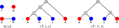
Figure 1: The induced cotree of a cograph $G$ affects the hc-coloring property of $\sigma$, where $\sigma(a)=\sigma(d)\neq\sigma(b)=\sigma(c)$. In $(T,t)$, the first tree from left to right, (K1)-(K3) are satisfied making $\sigma$ an hc-coloring. However the second tree $(T^{\prime},t^{\prime})$ does not satisfy (K3) since the parent node of $c\simeq K_{1}$ and $d\simeq K_{1}$ corresponds to a disjoint union operation and $\sigma(c)\cap\sigma(d)=\emptyset$. Thus $\sigma$ is not an hc-coloring w.r.t. $(T^{\prime},t^{\prime})$.

Theorem 2.1.

Let $\sigma:V\to S$ be an hc-coloring of a cograph $G$. Then $|S|=\chi(G)$.

Proof.

We proceed by induction w.r.t. $|V|$. The statement is trivially true for $|V|=1$, i.e. $G=K_{1}$, since $\chi(K_{1})=1$. Now suppose $|V|>1$. Thus $G=G_{1}\operatorname{\triangledown}G_{2}$ or $G=G_{1}\mathbin{\mathchoice{\leavevmode\vtop{\halign{\hfil$\m@th\displaystyle#$\hfil\cr\cup\cr\cdot\crcr}}}{\leavevmode\vtop{\halign{\hfil$\m@th\textstyle#$\hfil\cr\cup\cr\cdot\crcr}}}{\leavevmode\vtop{\halign{\hfil$\m@th\scriptstyle#$\hfil\cr\cup\cr\cdot\crcr}}}{\leavevmode\vtop{\halign{\hfil$\m@th\scriptscriptstyle#$\hfil\cr\cup\cr\cdot\crcr}}}}G_{2}$ for some graphs $G_{1}=(V_{1},E_{1})$ and $G_{1}=(V_{2},E_{2})$ with $1\leq|V_{1}|,|V_{2}|<|V|$. By induction hypothesis we have $|\sigma(V_{1})|=\chi(G_{1})$ and $|\sigma(V_{2})|=\chi(G_{2})$.

First consider $G=G_{1}\operatorname{\triangledown}G_{2}$. Since $xy\in E(G)$ for all $x\in V_{1}$ and $y\in V_{2}$ we have $\sigma(x)\neq\sigma(y)$, and hence $\sigma(V_{1})\cap\sigma(V_{2})=\emptyset$. Thus, $\sigma(V)=\sigma(V_{1})\mathbin{\mathchoice{\leavevmode\vtop{\halign{\hfil$\m@th\displaystyle#$\hfil\cr\cup\cr\cdot\crcr}}}{\leavevmode\vtop{\halign{\hfil$\m@th\textstyle#$\hfil\cr\cup\cr\cdot\crcr}}}{\leavevmode\vtop{\halign{\hfil$\m@th\scriptstyle#$\hfil\cr\cup\cr\cdot\crcr}}}{\leavevmode\vtop{\halign{\hfil$\m@th\scriptscriptstyle#$\hfil\cr\cup\cr\cdot\crcr}}}}\sigma(V_{2})$ and therefore,

$$|\sigma(V)|=|\sigma(V_{1})|+|\sigma(V_{2})|\stackrel{{\scriptstyle\text{IH.}}}{{=}}\chi(G_{1})+\chi(G_{2})\stackrel{{\scriptstyle\text{Equ.\ }\eqref{eq:rec1}}}{{=}}\chi(G).$$

We note that the coloring condition in (K2) therefore only enforces that $\sigma$ is a proper vertex coloring.

Now suppose $G=G_{1}\mathbin{\mathchoice{\leavevmode\vtop{\halign{\hfil$\m@th\displaystyle#$\hfil\cr\cup\cr\cdot\crcr}}}{\leavevmode\vtop{\halign{\hfil$\m@th\textstyle#$\hfil\cr\cup\cr\cdot\crcr}}}{\leavevmode\vtop{\halign{\hfil$\m@th\scriptstyle#$\hfil\cr\cup\cr\cdot\crcr}}}{\leavevmode\vtop{\halign{\hfil$\m@th\scriptscriptstyle#$\hfil\cr\cup\cr\cdot\crcr}}}}G_{2}$. Axiom (K3) implies $|\sigma(V)|=\max(|\sigma(V_{1})|,|\sigma(V_{2})|)$. Hence,

$$|\sigma(V)|=\max(|\sigma(V_{1})|,|\sigma(V_{2})|)\stackrel{{\scriptstyle\text{IH.}}}{{=}}\max(\chi(G_{1}),\chi(G_{2}))\stackrel{{\scriptstyle\text{Equ.\ }\eqref{eq:rec1}}}{{=}}\chi(G).$$

∎

As detailed in [2], we have $\chi(G)=\gamma(G)$. Thus, it seems natural to ask whether every greedy coloring is an hc-coloring. Making use of the fact that $\chi(G)=\gamma(G)$, we assume w.l.o.g. that the color set is $S=\{1,2,\dots,\chi(G)\}$ whenever we consider greedy colorings of a cograph. By definition of greedy colorings and the fact that cographs are hereditarily well-colored, we immediately observe

Lemma 2.2.

Let $\sigma$ be a greedy coloring of a cograph $G$ and $G_{1}=(V_{1},E_{1})$ a connected component of $G$. Then $G_{1}$ is colored by $\sigma(V_{1})=\{1,\dots,\chi(G_{1})\}$.

We shall say that a cograph $G$ is a minimal counterexample for some property $\mathcal{P}$ if (1) $G$ does not satisfy $\mathcal{P}$ and (2) every induced subgraph of $G$ (i.e., every “smaller” cograph) satisfies $\mathcal{P}$.

Lemma 2.3.

Let $G$ be a cograph, $(T,t)$ an arbitrary binary cotree for $G$ and $\sigma$ a greedy coloring of $G$. Then $\sigma$ is an hc-coloring w.r.t. $(T,t)$.

Proof.

Assume $G$ is a minimal counterexample, i.e., $G$ is a minimal cograph for which a coloring $\sigma$ exists that is a greedy coloring but not an hc-coloring. If $G$ is connected, then $G=\mathop{\vphantom{\sum}\mathchoice{\vbox{\hbox{\leavevmode\resizebox{9.00005pt}{}{$\triangledown$}}}}{\vbox{\hbox{\leavevmode\resizebox{10.00012pt}{}{$\triangledown$}}}}{\vbox{\hbox{\leavevmode\resizebox{7.00009pt}{}{$\triangledown$}}}}{\vbox{\hbox{\leavevmode\resizebox{5.00006pt}{}{$\triangledown$}}}}}\slimits@_{i=1}^{n}G_{i}$, for some $n>1$ and $\sigma(V)=\operatorname{\mathop{\vphantom{\bigcup}\mathchoice{\leavevmode\vtop{\halign{\hfil$\m@th\displaystyle#$\hfil\cr\bigcup\cr\cdot\crcr}}}{\leavevmode\vtop{\halign{\hfil$\m@th\textstyle#$\hfil\cr\bigcup\cr\cdot\crcr}}}{\leavevmode\vtop{\halign{\hfil$\m@th\scriptstyle#$\hfil\cr\bigcup\cr\cdot\crcr}}}{\leavevmode\vtop{\halign{\hfil$\m@th\scriptscriptstyle#$\hfil\cr\bigcup\cr\cdot\crcr}}}}\displaylimits}_{i=1}^{n}\sigma(V_{i})$, i.e., (K2) is satisfied. By assumption, $\sigma$ is not an hc-coloring, hence $\sigma$ must fail to be an hc-coloring on at least one of the connected components $G_{i}$, contradicting the assumption that $G$ is a minimal counterexample. Thus, $G$ cannot be connected.

Therefore, assume $G=\operatorname{\mathop{\vphantom{\bigcup}\mathchoice{\leavevmode\vtop{\halign{\hfil$\m@th\displaystyle#$\hfil\cr\bigcup\cr\cdot\crcr}}}{\leavevmode\vtop{\halign{\hfil$\m@th\textstyle#$\hfil\cr\bigcup\cr\cdot\crcr}}}{\leavevmode\vtop{\halign{\hfil$\m@th\scriptstyle#$\hfil\cr\bigcup\cr\cdot\crcr}}}{\leavevmode\vtop{\halign{\hfil$\m@th\scriptscriptstyle#$\hfil\cr\bigcup\cr\cdot\crcr}}}}\displaylimits}_{i=1}^{n}G_{i}$ for some $n>1$. Since $G$ is represented by a binary cotree $(T,t)$, the root of $T$ must have exactly two children $u$ and $v$. Hence, we can write $G=G(u)\mathbin{\mathchoice{\leavevmode\vtop{\halign{\hfil$\m@th\displaystyle#$\hfil\cr\cup\cr\cdot\crcr}}}{\leavevmode\vtop{\halign{\hfil$\m@th\textstyle#$\hfil\cr\cup\cr\cdot\crcr}}}{\leavevmode\vtop{\halign{\hfil$\m@th\scriptstyle#$\hfil\cr\cup\cr\cdot\crcr}}}{\leavevmode\vtop{\halign{\hfil$\m@th\scriptscriptstyle#$\hfil\cr\cup\cr\cdot\crcr}}}}G(v)$. Since $G$ is a minimal counterexample, we can conclude that $\sigma$ induces an hc-coloring on $G(u)$ and $G(v)$. However, since $\sigma$ is, in particular, a greedy coloring of $G(u)$ and $G(v)$, $\sigma(V(G(u)))\subseteq\sigma(V(G(v)))$ or $\sigma(V(G(v)))\subseteq\sigma(V(G(u)))$ most hold. But this immediately implies that $(G,\sigma)$ satisfies (K3) and thus $\sigma$ is an hc-coloring of $G$. Therefore, $G$ is not a minimal counterexample, which completes the proof. ∎

As an immediate consequence we find

Corollary 2.4.

Every cograph has an hc-coloring.

The converse of Lemma 2.3 is not true. Fig. 2 shows an example of an hc-coloring that is not a greedy coloring.

Figure 2: Both colorings A and B of $K_{2}\mathbin{\mathchoice{\leavevmode\vtop{\halign{\hfil$\m@th\displaystyle#$\hfil\cr\cup\cr\cdot\crcr}}}{\leavevmode\vtop{\halign{\hfil$\m@th\textstyle#$\hfil\cr\cup\cr\cdot\crcr}}}{\leavevmode\vtop{\halign{\hfil$\m@th\scriptstyle#$\hfil\cr\cup\cr\cdot\crcr}}}{\leavevmode\vtop{\halign{\hfil$\m@th\scriptscriptstyle#$\hfil\cr\cup\cr\cdot\crcr}}}}K_{1}\mathbin{\mathchoice{\leavevmode\vtop{\halign{\hfil$\m@th\displaystyle#$\hfil\cr\cup\cr\cdot\crcr}}}{\leavevmode\vtop{\halign{\hfil$\m@th\textstyle#$\hfil\cr\cup\cr\cdot\crcr}}}{\leavevmode\vtop{\halign{\hfil$\m@th\scriptstyle#$\hfil\cr\cup\cr\cdot\crcr}}}{\leavevmode\vtop{\halign{\hfil$\m@th\scriptscriptstyle#$\hfil\cr\cup\cr\cdot\crcr}}}}K_{1}$ are hc-colorings. However, only A is a greedy coloring since the two single-vertex components have different colors in B.

Theorem 2.5.

A coloring $\sigma$ of a cograph $G$ is greedy coloring if and only if it is an hc-coloring w.r.t. every binary cotree $(T,t)$ of $G$.

Proof.

By Lemma 2.3, every greedy coloring is an hc-coloring for every binary cotree $(T,t)$. Now suppose $\sigma$ is an hc-coloring for every binary cotree $(T,t)$ and let $G$ be a minimal cograph for which $\sigma$ is not a greedy coloring. As in the proof of Lemma 2.3 we can argue that $G$ cannot be a minimal counterexample if $G$ is connected: in this case, $G=\mathop{\vphantom{\sum}\mathchoice{\vbox{\hbox{\leavevmode\resizebox{9.00005pt}{}{$\triangledown$}}}}{\vbox{\hbox{\leavevmode\resizebox{10.00012pt}{}{$\triangledown$}}}}{\vbox{\hbox{\leavevmode\resizebox{7.00009pt}{}{$\triangledown$}}}}{\vbox{\hbox{\leavevmode\resizebox{5.00006pt}{}{$\triangledown$}}}}}\slimits@_{i=1}^{n}G_{i}$ and $\sigma(V)=\operatorname{\mathop{\vphantom{\bigcup}\mathchoice{\leavevmode\vtop{\halign{\hfil$\m@th\displaystyle#$\hfil\cr\bigcup\cr\cdot\crcr}}}{\leavevmode\vtop{\halign{\hfil$\m@th\textstyle#$\hfil\cr\bigcup\cr\cdot\crcr}}}{\leavevmode\vtop{\halign{\hfil$\m@th\scriptstyle#$\hfil\cr\bigcup\cr\cdot\crcr}}}{\leavevmode\vtop{\halign{\hfil$\m@th\scriptscriptstyle#$\hfil\cr\bigcup\cr\cdot\crcr}}}}\displaylimits}_{i=1}^{n}\sigma(V_{i})$ for all colorings, and thus $\sigma$ is a greedy coloring if and only if it is a greedy coloring with disjoint color sets for each $G_{i}$. Hence, a minimal counterexample must have at least two connected components.

Let $G=\operatorname{\mathop{\vphantom{\bigcup}\mathchoice{\leavevmode\vtop{\halign{\hfil$\m@th\displaystyle#$\hfil\cr\bigcup\cr\cdot\crcr}}}{\leavevmode\vtop{\halign{\hfil$\m@th\textstyle#$\hfil\cr\bigcup\cr\cdot\crcr}}}{\leavevmode\vtop{\halign{\hfil$\m@th\scriptstyle#$\hfil\cr\bigcup\cr\cdot\crcr}}}{\leavevmode\vtop{\halign{\hfil$\m@th\scriptscriptstyle#$\hfil\cr\bigcup\cr\cdot\crcr}}}}\displaylimits}_{i=1}^{n}G_{i}$ for some $n>1$ and define a partition of $\{1,\dots,n\}$ into sets $I_{1},\dots,I_{m}$, $m\geq 1$, such that for every $r\in\{1,\dots,m\}$, $i,j\in I_{r}$ if and only if $\chi(G_{i})=\chi(G_{j})$. Since every $G^{r}\coloneqq\operatorname{\mathop{\vphantom{\bigcup}\mathchoice{\leavevmode\vtop{\halign{\hfil$\m@th\displaystyle#$\hfil\cr\bigcup\cr\cdot\crcr}}}{\leavevmode\vtop{\halign{\hfil$\m@th\textstyle#$\hfil\cr\bigcup\cr\cdot\crcr}}}{\leavevmode\vtop{\halign{\hfil$\m@th\scriptstyle#$\hfil\cr\bigcup\cr\cdot\crcr}}}{\leavevmode\vtop{\halign{\hfil$\m@th\scriptscriptstyle#$\hfil\cr\bigcup\cr\cdot\crcr}}}}\displaylimits}_{i\in I_{r}}G_{i}$, $1\leq r\leq m$, is a cograph, each $G^{r}$ can be represented by a (not necessarily unique) binary cotree $(T^{r},t^{r})$. Note, we have $\chi(G^{r})=\chi(G_{i})$ for all $i\in I_{r}$. Now, we can construct a binary cotree $(T,t)$ for $G$ as follows: let $T^{*}$ be a caterpillar with leaf set $L(T^{*})=\{l_{1},\dots,l_{\ell}\}$. We choose $T^{*}=(\ldots((l_{1},l_{2}),l_{3}),\ldots l_{\ell})$ (in Newick format). Note, if $\ell=1$, then $T^{*}\simeq K_{1}$. Now, the root of every tree $T^{1},\dots,T^{r}$ is identified with a unique leaf in $L(T^{*})$ such that the root of $T_{i}$ is identified with $l_{i}\in L(T^{*})$ and the root of $T_{j}$ is identified with $l_{j}\in L(T^{*})$, where $i<j$ if and only if $\chi(G^{i})<\chi(G^{j})$. This yields the tree $T$. The labeling $t$ for $(T,t)$ is provided by keeping the labels of each $(T^{r},t^{r})$ and by labeling all other inner vertices of $T$ by $0$. It is easy to see that $(T,t)$ is a binary cotree for $G$. By hypothesis, this in particular implies that $\sigma$ is an hc-coloring w.r.t. $(T,t)$. We denote by $C(T^{*})\subseteq V(T)$ the set of inner vertices of $T^{*}$. Since $\sigma$ is an hc-coloring w.r.t. $(T,t)$ and thus in particular w.r.t. any subtree $(T^{r},t^{r})$, we have $\sigma(V(G_{i}))\cap\sigma(V(G_{j}))\in\{\sigma(V(G_{i})),\sigma(V(G_{j}))\}$ for any $i,j\in I_{r}$, $1\leq r\leq m$, by (K3). Hence, as $\chi(G^{r})=\chi(G_{i})=\chi(G_{j})$, it must necessarily hold $\sigma(V(G_{i}))=\sigma(V(G_{j}))$ for all $i,j\in I_{r}$, i.e., all connected components $G_{i}$ with the same chromatic number are colored by the same color set. By construction, at every node $v\in C(T^{*})$ of the caterpillar structure, with children $v^{\prime}$ and $v^{\prime\prime}$, the components $G^{\prime}:=G(v^{\prime})$ and $G^{\prime\prime}:=G(v^{\prime\prime})$ satisfy $\chi(G^{\prime})<\chi(G^{\prime\prime})$. Invoking (K3) we therefore have $\sigma(G^{\prime})\subset\sigma(G^{\prime\prime})$ and $G^{*}:=G(v)$ is colored by the color set $\sigma(G^{*})=\sigma(G^{\prime\prime})$. These set inclusions therefore imply a linear ordering of the colors such that colors in $\sigma(G^{\prime})$ come before those in $\sigma(G^{\prime\prime})\setminus\sigma(G^{\prime})$. Thus $\sigma$ is a greedy coloring provided that the restriction of $\sigma$ to each of the connected components $G_{i}$ of $G$ is a greedy coloring, which is true due to the assumption that $G$ is a minimal counterexample. Thus no minimal counterexample exists, and the coloring $\sigma$ is indeed a greedy coloring of $G$. ∎

Given an hc-cograph, it is not difficult to recover a corresponding binary cotree. To this end, we proceed top down. Denote the root of $(T,t)$ by $r$. It is associated with the graph $G(r)=G$. In the general step we consider an induced subgraph $G(u)$ of $G$ associated with a vertex $u$ of $T$. If $G(u)$ is connected, then $t(u)=1$ and $G(u)$ is the joint of pair of induced subgraphs $G(v_{1})$ and $G(v_{2})$. To identify these graphs, consider the connected components $\overline{G_{1}},\dots,\overline{G_{k}}$ of the complement $\overline{G(u)}$ of $G(u)$. We have

$$G(u)=\overline{\operatorname{\mathop{\vphantom{\bigcup}\mathchoice{\leavevmode\vtop{\halign{\hfil$\m@th\displaystyle#$\hfil\cr\bigcup\cr\cdot\crcr}}}{\leavevmode\vtop{\halign{\hfil$\m@th\textstyle#$\hfil\cr\bigcup\cr\cdot\crcr}}}{\leavevmode\vtop{\halign{\hfil$\m@th\scriptstyle#$\hfil\cr\bigcup\cr\cdot\crcr}}}{\leavevmode\vtop{\halign{\hfil$\m@th\scriptscriptstyle#$\hfil\cr\bigcup\cr\cdot\crcr}}}}\displaylimits}_{i=1}^{k}\overline{G_{i}}}=\mathop{\vphantom{\sum}\mathchoice{\vbox{\hbox{\leavevmode\resizebox{9.00005pt}{}{$\triangledown$}}}}{\vbox{\hbox{\leavevmode\resizebox{10.00012pt}{}{$\triangledown$}}}}{\vbox{\hbox{\leavevmode\resizebox{7.00009pt}{}{$\triangledown$}}}}{\vbox{\hbox{\leavevmode\resizebox{5.00006pt}{}{$\triangledown$}}}}}\slimits@_{i=1}^{k}\overline{\overline{G_{i}}}=\mathop{\vphantom{\sum}\mathchoice{\vbox{\hbox{\leavevmode\resizebox{9.00005pt}{}{$\triangledown$}}}}{\vbox{\hbox{\leavevmode\resizebox{10.00012pt}{}{$\triangledown$}}}}{\vbox{\hbox{\leavevmode\resizebox{7.00009pt}{}{$\triangledown$}}}}{\vbox{\hbox{\leavevmode\resizebox{5.00006pt}{}{$\triangledown$}}}}}\slimits@_{i=1}^{k}G_{i}\,.$$ (2)

We therefore set $G(v_{1})=G_{1}$ and $G(v_{2})=\overline{\operatorname{\mathop{\vphantom{\bigcup}\mathchoice{\leavevmode\vtop{\halign{\hfil$\m@th\displaystyle#$\hfil\cr\bigcup\cr\cdot\crcr}}}{\leavevmode\vtop{\halign{\hfil$\m@th\textstyle#$\hfil\cr\bigcup\cr\cdot\crcr}}}{\leavevmode\vtop{\halign{\hfil$\m@th\scriptstyle#$\hfil\cr\bigcup\cr\cdot\crcr}}}{\leavevmode\vtop{\halign{\hfil$\m@th\scriptscriptstyle#$\hfil\cr\bigcup\cr\cdot\crcr}}}}\displaylimits}_{i=2}^{k}\overline{G_{i}}}=\mathop{\vphantom{\sum}\mathchoice{\vbox{\hbox{\leavevmode\resizebox{9.00005pt}{}{$\triangledown$}}}}{\vbox{\hbox{\leavevmode\resizebox{10.00012pt}{}{$\triangledown$}}}}{\vbox{\hbox{\leavevmode\resizebox{7.00009pt}{}{$\triangledown$}}}}{\vbox{\hbox{\leavevmode\resizebox{5.00006pt}{}{$\triangledown$}}}}}\slimits@_{i=2}^{k}G_{i}$. By construction, we therefore have $G(u)=G(v_{1})\operatorname{\triangledown}G(v_{2})$ with disjoint color sets $\sigma(V(G(v_{1})))$. If $G(u)$ is disconnected, define $t(u)=0$, identify one of the components, say $G_{1}$, with the smallest numbers of colors $|\sigma(V(G_{1}))|$ and set $G(v_{1})=G_{1}$ and $G(v_{2})=G(u)\setminus G(v_{1})$. The fact that $G(u)$ is an hc-cograph ensures that $\sigma(V(G(v_{1})))\subseteq\sigma(V(G(v_{2})))$. In both the connected and the disconnected case we attach $v_{1}$ and $v_{2}$ as the children of $u$ in $T$. The reconstruction of $(T,t)$ can be preformed in linear time.

3 Recursively-Minimal Colorings

Not every minimal coloring of a cograph is an hc-coloring. For instance, if $G$ is a disconnected cograph, i.e., $G=\operatorname{\mathop{\vphantom{\bigcup}\mathchoice{\leavevmode\vtop{\halign{\hfil$\m@th\displaystyle#$\hfil\cr\bigcup\cr\cdot\crcr}}}{\leavevmode\vtop{\halign{\hfil$\m@th\textstyle#$\hfil\cr\bigcup\cr\cdot\crcr}}}{\leavevmode\vtop{\halign{\hfil$\m@th\scriptstyle#$\hfil\cr\bigcup\cr\cdot\crcr}}}{\leavevmode\vtop{\halign{\hfil$\m@th\scriptscriptstyle#$\hfil\cr\bigcup\cr\cdot\crcr}}}}\displaylimits}_{i=1}^{n}G_{i}$, then it suffices that $|\sigma(V_{i})|\leq\chi(G)$. In this case, we may use more colors than necessary on a connected component $G_{i}$ of $G$, resulting in $\chi(G_{i})\neq|\sigma(V_{i})|$. Thus, Theorem 2.1 implies that $\sigma$ is not an hc-coloring of $G_{i}$ and hence, by definition, not an hc-coloring of $G$. This suggests to consider another class of colored cographs.

Definition 3.1.

A color-minimal cograph $(G,\sigma)$ is either a $K_{1}$, the disjoint union of color-minimal cographs or the join of color-minimal cographs, and satisfies $|\sigma(V)|=\chi(G)$. A coloring $\sigma$ of a color-minimal cograph will be called recursively minimal.

Color-minimal cographs thus are those colorings for which every constituent in their construction along some binary cotree is colored with the minimal number of colors. Since every greedy coloring of every cograph satisfies this condition, every cograph has a recursively minimal coloring.

Theorem 3.1.

Let $G$ be a cograph. A coloring $\sigma$ of $G$ is recursively minimal if and only it is an hc-coloring.

Proof.

Since every hc-coloring $\sigma$ of a cograph $G$ uses exactly $\chi(G)$ colors, the recursive definition of hc-colorings immediately implies that $\sigma$ is recursively minimal.

Now suppose there is a minimal cograph $G$ with a coloring $\sigma$ that is recursively minimal but not an hc-coloring. If $G$ is connected, then $G=\mathop{\vphantom{\sum}\mathchoice{\vbox{\hbox{\leavevmode\resizebox{9.00005pt}{}{$\triangledown$}}}}{\vbox{\hbox{\leavevmode\resizebox{10.00012pt}{}{$\triangledown$}}}}{\vbox{\hbox{\leavevmode\resizebox{7.00009pt}{}{$\triangledown$}}}}{\vbox{\hbox{\leavevmode\resizebox{5.00006pt}{}{$\triangledown$}}}}}\slimits@_{i=1}^{n}G_{i}$ for some $n\geq 2$ and the restrictions of $\sigma$ to the connected components $G_{i}$ use disjoint color sets. Hence, $\sigma$ is an hc-coloring whenever the restriction to each $G_{i}$ is an hc-coloring. Thus a minimal counterexample cannot be connected. Now suppose $G=\operatorname{\mathop{\vphantom{\bigcup}\mathchoice{\leavevmode\vtop{\halign{\hfil$\m@th\displaystyle#$\hfil\cr\bigcup\cr\cdot\crcr}}}{\leavevmode\vtop{\halign{\hfil$\m@th\textstyle#$\hfil\cr\bigcup\cr\cdot\crcr}}}{\leavevmode\vtop{\halign{\hfil$\m@th\scriptstyle#$\hfil\cr\bigcup\cr\cdot\crcr}}}{\leavevmode\vtop{\halign{\hfil$\m@th\scriptscriptstyle#$\hfil\cr\bigcup\cr\cdot\crcr}}}}\displaylimits}_{i=1}^{n}G_{i}$ for some $n\geq 2$. Since $(G,\sigma)$ is by assumption a minimal counterexample, each connected component $(G_{i},\sigma_{i})$ is an hc-cograph. By Equ. (1) there is a connected component, say w.l.o.g. $G_{1}$, such that $\chi(G)=\chi(G_{1})$. By definition, $\sigma$ induces a recursively minimal coloring $\sigma_{1}$ on $G_{1}$ and $\sigma^{\prime}$ on $G^{\prime}=\operatorname{\mathop{\vphantom{\bigcup}\mathchoice{\leavevmode\vtop{\halign{\hfil$\m@th\displaystyle#$\hfil\cr\bigcup\cr\cdot\crcr}}}{\leavevmode\vtop{\halign{\hfil$\m@th\textstyle#$\hfil\cr\bigcup\cr\cdot\crcr}}}{\leavevmode\vtop{\halign{\hfil$\m@th\scriptstyle#$\hfil\cr\bigcup\cr\cdot\crcr}}}{\leavevmode\vtop{\halign{\hfil$\m@th\scriptscriptstyle#$\hfil\cr\bigcup\cr\cdot\crcr}}}}\displaylimits}_{i=2}^{n}G_{i}$. Since $G$ is a minimal counterexample, $\sigma_{1}$ and $\sigma^{\prime}$ are hc-colorings of $G_{1}$ and $G^{\prime}$, respectively, in other words $(G_{1},\sigma_{1})$ and $(G^{\prime},\sigma^{\prime})$ are hc-cographs. Moreover, $\chi(G)=\chi(G_{1})$ implies $\sigma^{\prime}(V(G^{\prime}))\subseteq\sigma_{1}(V(G_{1}))$. In summary, therefore, $(G,\sigma)=(G_{1},\sigma_{1})\mathbin{\mathchoice{\leavevmode\vtop{\halign{\hfil$\m@th\displaystyle#$\hfil\cr\cup\cr\cdot\crcr}}}{\leavevmode\vtop{\halign{\hfil$\m@th\textstyle#$\hfil\cr\cup\cr\cdot\crcr}}}{\leavevmode\vtop{\halign{\hfil$\m@th\scriptstyle#$\hfil\cr\cup\cr\cdot\crcr}}}{\leavevmode\vtop{\halign{\hfil$\m@th\scriptscriptstyle#$\hfil\cr\cup\cr\cdot\crcr}}}}(G^{\prime},\sigma^{\prime})$ satisfies (K3), thus it is a cograph with hc-coloring $\sigma$. Hence, there cannot exist a minimal cograph with a coloring $\sigma$ that is recursively minimal but not an hc-coloring. ∎

Recursively minimal colorings can be constructed in a very simply manner by stepwisely relabeling colors of disconnected subgraphs as outlined in Alg. 1.

Algorithm 1 Recursively minimal coloring of a cograph

0  Cograph $G$

1  $(T_{G},t_{G})\leftarrow$ discriminating cotree of $G$

2  initialize all $v\in V(G)$ with different colors

3  for all $v\in V^{0}(T_{G})$, from bottom to top do

4     if $t(v)=0$ then

5        $\mathcal{G}\leftarrow$ set of connected components of $G(v)$

6        $G^{*}\leftarrow\operatorname*{arg\,max}_{G_{i}\in\mathcal{G}}\chi(G_{i})$

7        $S\leftarrow\sigma(V(G^{*}))$

8        for all $G_{j}\in\mathcal{G},G_{j}\neq G^{*}$ do

9           randomly choose an injective map $\phi:\sigma(V(G_{j}))\to S$

10           for all $x\in V(G_{j})$ do

11              $\sigma(x)\leftarrow\phi(\sigma(x))$

Theorem 3.2.

Given a cograph $G$, Algorithm 1 returns a recursively minimal coloring of $G$. Moreover, every recursively minimal coloring of a cograph $G$ can be constructed with this algorithm.

Proof.

The bottom-up traversal of the cotree ensures that for every inner vertex $v$ of $T_{G}$, the subgraphs induced by its children ${v_{1},...,v_{j}}$ are color-minimal cographs. In particular this means that $|\sigma(V(G(v_{i}))|=\chi(G(v_{i}))$ for all $i\in\{1,..,j\}$. Take an arbitrary $v\in V^{0}(G)$. Suppose $t(v)=0$. The fact that $T_{G}$ is a discriminating cotree implies that all $t(v_{i})=1$, for all $i\in\{1,..,j\}$, and therefore $G_{i}:=G(v_{i})$ are connected components. Futhermore, there exists a $G_{k}$ such that $\chi(G_{k})=\max_{i}\chi(G_{i})$. These observations and Equ. (1) guarantee that lines 5-7 obtain a set of color $S$ such that $|S|=\chi(G(v))$. Explicitly, $\chi(G(v))=\chi(G_{k})$ and $S=\sigma(V(G_{k}))$. An injective recoloring $\phi:\sigma(V(G_{i}))\rightarrow S$, in lines 8-11, assures that $\sigma(G_{i})\subseteq S$ and therefore $\sigma(V(G(v))=S$. This implies that $G(v)$ is a color-minimal cograph with $\sigma$ a recursively minimal coloring. The converse is followed by the fact that every recursively minimal coloring can be obtained with a particular injection $\phi$. ∎

Algorithm 1 can be modified easily to construct a recursively minimal coloring of $G$ with respect to a user defined cotree $(T,t)$. It suffices to replace the connected components of $G(v)$ by the (not necessarily connected) induced subgraphs $G(w)$ corresponding to the children of $v$. Since $\chi(G(v))=\max_{w\in\mathsf{child}(v)}\chi(G(w))$, it suffices to choose the color set of the child that uses the largest number of colors and re-color all other child-graphs with this color set. For completeness, we summarize this variant in Algorithm 2.

Algorithm 2 Recursively minimal coloring of a cograph w.r.t. a given cotree.

0  Cograph $G$ and co-tree $(T,t)$

1  initialize all $v\in V(G)$ with different colors

2  for all $v\in V^{0}(T)$, from bottom to top do

3     if $t(v)=0$ then

4        $\mathcal{G}\leftarrow\{G(w)\colon w\in\mathsf{child}(v)\}$

5        $G^{*}\leftarrow\operatorname*{arg\,max}_{w\in\mathsf{child}(v)}|\chi(G(w))|$

6        $S\leftarrow\sigma(V(G^{*}))$

7        for all $G_{j}\in\mathcal{G},G_{j}\neq G^{*}$ do

8           randomly choose an injective map $\phi:\sigma(G_{j})\to S$

9           for all $x\in V(G_{j})$ do

10              $\sigma(x)\leftarrow\phi(\sigma(x))$

The recursive structure of hc-cographs can also be used to count the number of distinct hc-colorings of a cograph $G$ that is explained by a cotree $(T,t)$. For an inner vertex $u$ of $T$ denote by $N(G(u))$ the number of hc-colorings of $G(u)$. If $u$ is a leaf, then $N(u)=1$. Recall that $T$ is binary by Def. 1.2, i.e., $\mathsf{child}(u)=\{v_{1},v_{2}\}$. For $t(u)=1$, we have $N(G(u))=N(G(v_{1}))N(G(v_{2}))$ since the color sets are disjoint. If $t(u)=0$, assume, w.l.o.g. $s_{1}:=|\sigma(G(v_{1}))|\leq|\sigma(G(v_{2}))|=:s_{2}$, $N(G(u))=N(G(v_{1}))N(G(v_{2}))g(s_{1},s_{2})$, where $g(s_{1},s_{2})$ is the number of injections between a set of size $s_{1}$ into a set of size $s_{2}$, i.e., $g(s_{1},s_{2})=\binom{s_{2}}{s_{1}}s_{1}!$.

The total number of hc-colorings can be obtained by considering a caterpillar tree for the step-wise union of connected components. For each connected component $G_{i}$ with $\chi(G_{i})=s_{i}$, and $s=\max_{i}s_{i}$ there are $\binom{s}{s_{i}}$ choices of the colors, i.e., $g(s,s_{i})$ injections and thus $N(G)=\prod_{i}g(s,s_{i})N(G_{i})$ colorings. We note in passing that the chromatic polynomial of a cograph, and thus the number of colorings using the minimal number of colors, can be computed in polynomial time [8]. There does not seem to be an obvious connection between the hc-colorings and the chromatic polynomial, however.

4 Concluding Remarks

The cotrees $(T,t)$ associated with a cograph are a special case of the modular decomposition tree [4], which in addition to disjoint unions and joins also contains so-called prime nodes. The latter have a special structure known as spiders, which also admit a well-defined unique decomposition in so-called $P_{4}$-sparse graphs [6]. For this type of graphs it also makes sense to consider recursively minimal colorings. More generally, many interesting classes of graphs admit recursive constructions [10, 9]. For every graph class that has a recursive construction, one can ask whether minimal colorings can be constructed from optimal colorings, i.e., whether recursively minimal colorings exist. In some cases, such Cartesian products of graphs, where $\chi(G)$ equals the maximum of the chromatic numbers of the factors [11], this seems rather straightforward. In general, however, the answer is probably negative.

Acknowledgments

This work was support in part by the German Federal Ministry of Education and Research (BMBF, project no. 031A538A, de.NBI-RBC) and the Mexican Consejo Nacional de Ciencia y Tecnología (CONACyT, 278966 FONCICYT2).

References

• [1] Sebastian Böcker and Andreas W. M. Dress. Recovering symbolically dated, rooted trees from symbolic ultrametrics. Adv. Math., 138:105–125, 1998.
• [2] C. A. Christen and S. M. Selkow. Some perfect coloring properties of graphs. J. Comb. Th., Ser. B, 27:49–59, 1979.
• [3] D. G. Corneil, H. Lerchs, and L. Steward Burlingham. Complement reducible graphs. Discr. Appl. Math., 3:163–174, 1981.
• [4] T. Gallai. Transitiv orientierbare graphen. Acta Math Acad. Sci. Hungaricae, 18:25–66, 1967.
• [5] Manuela Geiß, Marc Hellmuth, and Peter F. Stadler. Reciprocal best match graphs. 2019. submitted, arxiv q-bio 1903.07920.
• [6] B. Jamison and S. Olariu. A tree representation for $p_{4}$-sparse graphs. Discrete Appl. Math., 35:115–129, 1992.
• [7] Richard M. Karp. Reducibility among combinatorial problems. In R E Miller, J W Thatcher, and J D Bohlinger, editors, Complexity of Computer Computations, pages 85–103. Plenum, New York, 1972.
• [8] J. A. Makowsky, U. Rotics, I. Averbouch, and B. Godlin. Computing graph polynomials on graphs of bounded clique-width. In F. V. Fomin, editor, Graph-Theoretic Concepts in Computer Science, volume 4271 of Lecture Notes Comp. Sci., pages 191–204, Berlin, Heidelberg, 2006. Springer.
• [9] Marc Noy and Ares Ribó. Recursively constructible families of graphs. Adv. Appl. Math., 32:350–363, 2004.
• [10] Andrzej Proskurowski. Recursive graphs, recursive labelings and shortest paths. SIAM J. Comput., 10:391–397, 1981.
• [11] Gerd Sabidussi. Graphs with given group and given graph-theoretical properties. Canad. J. Math., 9:515–525, 1957.
• [12] Manouchehr Zaker. Results on the Grundy chromatic number of graphs. Discr. Math., 306:3166–3173, 2006.