Learning Latent Trees with Stochastic Perturbations
and Differentiable Dynamic Programming

Abstract

We treat projective dependency trees as latent variables in our probabilistic model and induce them in such a way as to be beneficial for a downstream task, without relying on any direct tree supervision. Our approach relies on Gumbel perturbations and differentiable dynamic programming. Unlike previous approaches to latent tree learning, we stochastically sample global structures and our parser is fully differentiable. We illustrate its effectiveness on sentiment analysis and natural language inference tasks. We also study its properties on a synthetic structure induction task. Ablation studies emphasize the importance of both stochasticity and constraining latent structures to be projective trees.

1 Introduction

Discrete structures are ubiquitous in the study of natural languages, for example in morphology, syntax and discourse analysis. In natural language processing, they are often used to inject linguistic prior knowledge into statistical models. For examples, syntactic structures have been shown beneficial in question answering Cui et al. (2005), sentiment analysis Socher et al. (2013), machine translation Bastings et al. (2017) and relation extraction Liu et al. (2015), among others. However, linguistic tools producing these structured representations (e.g., syntactic parsers) are not available for many languages and not robust when applied outside of the domain they were trained on  Petrov et al. (2010); Foster et al. (2011). Moreover, linguistic structures do not always seem suitable in downstream applications, with simpler alternatives sometimes yielding better performance Wang et al. (2018).

Indeed, a parallel line of work focused on inducing task-specific structured representations of language Naradowsky et al. (2012); Yogatama et al. (2017); Kim et al. (2017); Liu and Lapata (2018); Niculae et al. (2018). In these approaches, no syntactic or semantic annotation is needed for training: representation is induced from scratch in an end-to-end fashion, in such a way as to benefit a given downstream task. In other words, these approaches provide an inductive bias specifying that (hierarchical) structures are appropriate for representing a natural language, but do not make any further assumptions regarding what the structures represent. Structures induced in this way, though useful for the task, tend not to resemble any accepted syntactic or semantic formalisms Williams et al. (2018a). Our approach falls under this category.

In our method, projective dependency trees (see Figure 3 for examples) are treated as latent variables within a probabilistic model. We rely on differentiable dynamic programming Mensch and Blondel (2018) which allows for efficient sampling of dependency trees Corro and Titov (2019). Intuitively, sampling a tree involves stochastically perturbing dependency weights and then running a relaxed form of the Eisner dynamic programming algortihm Eisner (1996). A sampled tree (or its continuous relaxation) can then be straightforwardly integrated in a neural sentence encoder for a target task using graph convolutional networks (GCNs, Kipf and Welling, 2017). The entire model, including the parser and GCN parameters, are estimated jointly while minimizing the loss for the target task.

What distinguishes us from previous work is that we stochastically sample global structures and do it in a differentiable fashion. For example, the structured attention method Kim et al. (2017); Liu and Lapata (2018) does not sample entire trees but rather computes arc marginals, and hence does not faithfully represent higher-order statistics. Much of other previous work relies either on reinforcement learning Yogatama et al. (2017); Nangia and Bowman (2018); Williams et al. (2018a) or does not treat the latent structure as a random variable Peng et al. (2018). Niculae et al. (2018) marginalizes over latent structures, however, this necessitates strong sparsity assumptions on the posterior distributions which may inject undesirable biases in the model. Overall, differential dynamic programming has not been actively studied in the task-specific tree induction context. Most previous work also focused on constituent trees rather than dependency ones.

We study properties of our approach on a synthetic structure induction task and experiment on sentiment classification Socher et al. (2013) and natural language inference Bowman et al. (2015). Our experiments confirm that the structural bias encoded in our approach is beneficial. For example, our approach achieves a 4.9% improvement on multi-genre natural language inference (MultiNLI) over a structure-agnostic baseline. We show that stochastisticity and higher-order statistics given by the global inference are both important. In ablation experiments, we also observe that forcing the structures to be projective dependency trees rather than permitting any general graphs yields substantial improvements without sacrificing execution time. This confirms that our inductive bias is useful, at least in the context of the considered downstream applications. Our main contributions can be summarized as follows:

1. we show that a latent tree model can be estimated by drawing global approximate samples via Gumbel perturbation and differentiable dynamic programming;

2. we demonstrate that constraining the structures to be projective dependency trees is beneficial;

3. we show the effectiveness of our approach on two standard tasks used in latent structure modelling and on a synthetic dataset.

2 Background

In this section, we describe the dependency parsing problem and GCNs which we use to incorporate latent structures into models for downstream tasks.

2.1 Dependency Parsing

Dependency trees represent bi-lexical relations between words. They are commonly represented as directed graphs with vertices and arcs corresponding to words and relations, respectively.

Let $x=x_{0}\ldots x_{n}$ be an input sentence with $n$ words where $x_{0}$ is a special root token. We describe a dependency tree of $x$ with its adjacency matrix ${\bm{T}}\in\{0,1\}^{n\times n}$ where ${T}_{h,m}=1$ iff there is a relation from head word $x_{h}$ to modifier word $x_{m}$. We write $\mathcal{T}(x)$ to denote the set of trees compatible with sentence $x$.

We focus on projective dependency trees. A dependency tree ${\bm{T}}$ is projective iff for every arc ${T}_{h,m}=1$, there is a path with arcs in ${\bm{T}}$ from $x_{h}$ to each word $x_{i}$ such that $h<i<m$ or $m<i<h$. Intuitively, a tree is projective as long as it can be drawn above the words in such way that arcs do not cross each other (see Figure 3). Similarly to phrase-structure trees, projective dependency trees implicitly encode hierarchical decomposition of a sentence into spans (‘phrases’). Forcing trees to be projective may be desirable as even flat span structures can be beneficial in applications (e.g., encoding multi-word expressions). Note that actual syntactic trees are also, to a large degree, projective, especially for such morphologically impoverished languages as English. Moreover, restricting the space of the latent structures is important to ease their estimation. For all these reasons, in this work we focus on projective dependency trees.

In practice, a dependency parser is given a sentence $x$ and predicts a dependency tree ${\bm{T}}\in\mathcal{T}(x)$ for this input. To this end, the first step is to compute a matrix ${\bm{W}}\in\mathbb{R}^{n\times n}$ that scores each dependency. In this paper, we rely on a deep dotted attention network. Let ${\bm{e}}_{0}\ldots{\bm{e}}_{n}$ be embeddings associated with each word of the sentence. We follow Parikh et al. (2016) and compute the score for each head-modifier pair $(x_{h},x_{m})$ as follows:

$${W}_{h,m}\!=\!\mathrm{MLP}^{\text{head}}({\bm{e}}_{h})\!^{\top}\!\mathrm{MLP}^{\text{mod}}({\bm{e}}_{m}\!)\!+\!b_{h{\text{-}}m},$$ (1)

where $\mathrm{MLP}^{\text{head}}$ and $\mathrm{MLP}^{\text{mod}}$ are multilayer perceptrons, and $b_{h{\text{-}}m}$ is a distance-dependent bias, letting the model encode preference for long or short-distance dependencies. The conditional probability of a tree $p_{\theta}({\bm{T}}|x)$ is defined by a log-linear model:

$$p_{\theta}({\bm{T}}|x)=\frac{\exp(\sum_{h,m}{W}_{h,m}{T}_{h,m})}{\sum_{T^{\prime}\in\mathcal{T}(x)}\exp(\sum_{h,m}{W}_{h,m}{T}^{\prime}_{h,m})}.$$

When tree annotation is provided in data ${\mathbb{D}}$, networks parameters $\theta$ are learned by maximizing the log-likelihood of annotated trees Lafferty et al. (2001).

The highest scoring dependency tree can be produced by solving the following mathematical program:

$$\bm{T}=\operatorname*{arg\,max}_{\bm{T}\in\mathcal{T}(\bm{x})}\quad\sum_{h,m}{W}_{h,m}{T}_{h,m}.$$ (2)

If $\mathcal{T}(\bm{x})$ is restricted to be the set of projective dependency trees, this can be done efficiently in $O(n^{3})$ using the dynamic programming algorithm of Eisner (1996).

2.2 Graph Convolutional Networks

Graph Convolutional Networks (GCNs, Kipf and Welling, 2017; Marcheggiani and Titov, 2017) compute context-sensitive embeddings with respect to a graph structure. GCNs are composed of several layers where each layer updates vertices representations based on the current representations of their neighbors. In this work, we fed the GCN with word embeddings and a tree sample ${\bm{T}}$. For each word $x_{i}$, a GCN layer produces a new representation relying both on word embedding of $x_{i}$ and on embeddings of its heads and modifiers in ${\bm{T}}$. Multiple GCN layers can be stacked on top of each other. Therefore, a vertex representation in a GCN with $k$ layers is influenced by all vertices at a maximum distance of $k$ in the graph. Our GCN is sensitive to arc direction.

More formally, let ${\bm{E}}^{0}={\bm{e}}_{0}\odot\dots\odot{\bm{e}}_{n}$, where $\odot$ is the column-wise concatenation operator, be the input matrix with each column corresponding to a word in the sentence. At each GCN layer $t$, we compute:

$${\bm{E}}^{t+1}=\sigma\left(f({\bm{E}}^{t})+g({\bm{E}}^{t}){\bm{T}}+h({\bm{E}}^{t}){\bm{T}}^{\top}\right),$$

where $\sigma$ is an activation function, e.g. $\mathrm{ReLU}$. Functions $f()$, $g()$ and $h()$ are distinct multi-layer perceptrons encoding different types of relationships: self-connection, head and modifier, respectively (hyperparameters are provided in Appendix A). Note that each GCN layer is easily parallelizable on GPU both over vertices and over batches, either with latent or predefined structures.

(a)

(b)

Figure 1: The two directed graphical models used in this work. Shaded and unshaded nodes represent observable and unobservable variables, respectively. LABEL:sub@fig:network:sst In the sentence classification task, the output $y$ is conditioned on the input and the latent tree. LABEL:sub@fig:network:snli In the natural language inference task, the output is conditioned on two sentences and their respective latent trees.

3 Structured Latent Variable Models

In the previous section, we explained how a dependency tree is produced for a given sentence and how we extract features from this tree with a GCN. In our model, we assume that we do not have access to gold-standard trees and that we want to induce the best structure for the downstream task. To this end, we introduce a probability model where the dependency structure is a latent variable (Section 3.1). The distribution over dependency trees must be inferred from the data (Section 3.2). This requires marginalization over dependency trees during training, which is intractable due to the large search space. Instead, we rely on Monte-Carlo (MC) estimation.

3.1 Graphical Model

Let $x$ be the input sentence, $y$ be the output (e.g. sentiment labelling) and $\mathcal{T}(x)$ be the set of latent structures compatible with input $x$. We construct a directed graphical model where $x$ and $y$ are observable variables, i.e. their values are known during training. However, we assume that the probability of the output $y$ is conditioned on a latent tree ${\bm{T}}\in\mathcal{T}(x)$, a variable that is not observed during training: it must be inferred from the data. Formally, the model is defined as follows:

$$p_{\theta}(y|x) =\mathbb{E}_{p_{\theta}({\bm{T}}|x)}[p(y|x,{\bm{T}})]$$ (3)

$$=\sum_{{\bm{T}}\in\mathcal{T}(x)}p_{\theta}({\bm{T}}|x)\times p_{\theta}(y|x,{\bm{T}}),$$

where $\theta$ denotes all the parameters of the model. An illustration of the network is given in Figure 1a.

3.2 Parameter Estimation

Our probability distributions are parameterized by neural networks. Their parameters $\theta$ are learned via gradient-based optimization to maximize the log-likelihood of (observed) training data. Unfortunately, estimating the log-likelihood of observation requires computing the expectation in Equation 3, which involves an intractable sum over all valid dependency trees. Therefore, we propose to optimize a lower bound on the log-likelihood, derived by application of Jensen’s inequality which can be efficiently estimated with the Monte-Carlo (MC) method:

$$\log \;p_{\theta}(y^{i}|x^{i})=\log\mathbb{E}_{{\bm{T}}\sim p_{\theta}({\bm{T}}|x^{i})}[p_{\theta}(y^{i}|{\bm{T}},x^{i})]$$

$$\geq\mathbb{E}_{{\bm{T}}\sim p_{\theta}({\bm{T}}|x^{i})}[\log p_{\theta}(y^{i}|{\bm{T}},x^{i})].$$ (4)

However, MC estimation introduces a non-differentiable sampling function ${\bm{T}}\sim p_{\theta}({\bm{T}}|x^{i})$ in the gradient path. Score function estimators have been introduced to bypass this issue but suffer from high variance Williams (1987); Fu (2006); Schulman et al. (2015). Instead, we propose to reparametrize the sampling process Kingma and Welling (2014), making it independent of the learned parameter $\theta$ : in such case, the sampling function is outside of the gradient path. To this end, we rely on the Perturb-and-MAP framework Papandreou and Yuille (2011). Specifically, we perturb the potentials (arc weights) with samples from the Gumbel distribution and compute the most probable structure with the perturbed potentials:

$${G}_{h,m} \sim\mathcal{G}(0,1),$$ (5)

$$\widetilde{{\bm{W}}} ={\bm{W}}+{\bm{G}},$$ (6)

$${\bm{T}} =\operatorname*{arg\,max}_{{\bm{T}}\in\mathcal{T}(x)}\sum_{h,m}{T}_{h,m}\widetilde{{W}}_{h,m}.$$ (7)

Each element of the matrix ${\bm{G}}\in\mathbb{R}^{n\times n}$ contains random samples from the Gumbel distribution which is independent from the network parameters $\theta$, hence there is no need to backpropagate through this path in the computation graph. Note that, unlike the Gumbel-Max trick Maddison et al. (2014), sampling with Perturb-and-MAP is approximate, as the noise is factorizable: we add noise to individual arc weights rather than to scores of entire trees (which would not be tractable). This is the first source of bias in our gradient estimator. The maximization in Equation 7 can be computed using the algorithm of Eisner (1996). We stress that the marginalization in Equation 3 and MC estimated sum over trees capture high-order statistics, which is fundamentally different from computing edge marginals, i.e. structured attention Kim et al. (2017). Unfortunately, the estimated gradient of the reparameterized distribution over parse trees is ill-defined (either undefined or null). We tackle this issue in the following section.

1:function build-uright($i,j,\widetilde{{\bm{W}}}$)

2:     ${\bm{s}}\leftarrow$ null-initialized vec. of size $j-i$

3:     for $i\leq k<j$ do

4:          ${s}_{i-k}$ $\leftarrow$ $[i,k,\rightarrow,\top]+[k+1,j,\leftarrow,\top]$      

5:     ${\bm{b}}\leftarrow$ one-hot-argmax(${\bm{s}}$)

6:     $\textsc{backptr}[i,j,\rightarrow,\bot]$ $\leftarrow$ ${\bm{b}}$

7:     $\textsc{weight}[i,j,\rightarrow,\bot]$ $\leftarrow$ ${\bm{b}}^{\top}{\bm{s}}+{W}_{j,i}$

Algorithm 1 This function computes the chart values for items of the form $[i,j,\rightarrow,\bot]$ by searching the set of antecedents that maximizes its score. Because these items assume a dependency from $x_{i}$ to $x_{j}$, we add ${W}_{i,h}$ to the score.

1:function Backtrack-uright($i,j,{\bm{T}}$)

2:     ${T}_{i,j}\leftarrow\textsc{contrib}[i,j,\rightarrow,\bot]$

3:     ${\bm{b}}\leftarrow\textsc{backptr}[i,j,\rightarrow,\bot]$

4:     for $i\leq k<j$ do

5:         $\textsc{contrib}[i,k,\rightarrow,\top]\overset{+}{\leftarrow}{b}_{i-k}{T}_{i,j}$

6:         $\textsc{contrib}[k+1,j,\leftarrow,\top]\overset{+}{\leftarrow}{b}_{i-k}{T}_{i,j}$      

Algorithm 2 If item $[i,j,\rightarrow,\bot]$ has contributed the optimal objective, this function sets ${T}_{i,j}$ to $1$. Then, it propagates the contribution information to its antecedents.

4 Differentiable Dynamic Programming

Neural networks parameters are learned using (variants of) the stochastic gradient descent algorithm. The gradient is computed using the back-propagation algorithm that rely on partial derivative of each atomic operation in the network. The perturb-and-MAP sampling process relies on the dependency parser (Equation 7) which contains ill-defined derivatives. This is due to the usage of constrained $\operatorname*{arg\,max}$ operations Gould et al. (2016); Mensch and Blondel (2018) in the algorithm of Eisner (1996). Let $\mathcal{L}$ be the training loss, backpropagation is problematic because of the following operation:

$$\frac{\partial\mathcal{L}}{\partial\widetilde{{\bm{W}}}}=\frac{\partial\mathcal{L}}{\partial{\bm{T}}}\frac{\partial{\bm{T}}}{\partial\widetilde{{\bm{W}}}}$$

where $\frac{\partial{\bm{T}}}{\partial\widetilde{{\bm{W}}}}$ is the partial derivative with respect to the dependency parser (Equation 7) which is null almost everywhere, i.e. there is no descent direction information. We follow previous work and use a differentiable dynamic programming surrogate Mensch and Blondel (2018); Corro and Titov (2019). The use of the surrogate is the second source of bias in our gradient estimation.

4.1 Parsing with Dynamic Programming

The projective dependency parser of Eisner (1996) is a dynamic program that recursively builds a chart of items representing larger and larger spans of the input sentence. Items are of the form $[i,j,d,c]$ where: $0\leq i\leq j\leq n$ are the boundaries of the span; $d\in\{\rightarrow,\leftarrow\}$ is the direction of the span, i.e. a right span $\rightarrow$ (resp. left span $\leftarrow$) means that all the words in the span are descendants of $x_{i}$ (resp. $x_{j}$) in the dependency tree; $c\in\{\top,\bot\}$ indicates if the span is complete ($\top$) or incomplete ($\bot$) in its direction. In a complete right span, $x_{j}$ cannot have any modifiers on its right side. In a complete left span, $x_{i}$ cannot have any modifier on its left side. A set of deduction rules defines how the items can be deduced from their antecedents.

The algorithm consists of two steps. In the first step, items are deduced in a bottom-up fashion and the following information is stored in the chart: the maximum weight that can be obtained by each item and backpointers to the antecedents that lead to this maximum weight (Algorithm 1). In the second step, the backpointers are used to retrieve the items corresponding to the maximum score and values in ${\bm{T}}$ are set accordingly (Algorithm 2).

4.2 Continuous Relaxation

The $\operatorname*{one-hot-argmax}$ operation on line 5 in Algorithm 1 can be written as follows:

$$\operatorname*{arg\,max}_{{\bm{b}}\geq 0}\quad\sum_{k}{b}_{k}{s}_{k} \text{s.t.}\sum_{k}{b}_{k}=1.$$

It is known that a continuous relaxation of $$\operatorname*{arg\,max}$$ in the presence of inequality constraints can be obtained by introducing a penalizer that prevents activation of inequalities at the optimal solutions Gould et al. (2016):

$$\operatorname*{arg\,max}_{{\bm{b}}\geq 0}\quad\sum_{k}{b}_{k}{s}_{k}-\Omega({\bm{b}}) \text{s.t.}\sum_{k}{b}_{k}=1.$$

Several $\Omega$ functions have been studied in the literature for different purposes, including logarithmic and inverse barriers for the interior point method Den Hertog et al. (1994); Potra and Wright (2000) and negative entropy for deterministic annealing Rangarajan (2000). When using negative entropy, i.e. $\Omega({\bm{b}})=\sum_{k}{b}_{k}\log{b}_{k}$, solving the penalized $\operatorname*{one-hot-argmax}$ has a closed form solution that can be computed using the $\mathrm{softmax}$ function Boyd and Vandenberghe (2004), that is:

$${b}_{k}=\frac{\exp({s}_{k})}{\sum_{k^{\prime}}\exp({s}_{k^{\prime}})}.$$

Therefore, we replace the non-differentiable $\operatorname*{one-hot-argmax}$ operation in Algorithm 1 with a softmax in order to build a smooth and fully differentiable surrogate of the parsing algorithm.s

5 Controlled Experiment

We first experiment on a toy task. The task is designed in such a way that there exists a simple projective dependency grammar which turns it into a trivial problem. We can therefore perform thorough analysis of the latent tree induction method.

5.1 Dataset and Task

The ListOps dataset Nangia and Bowman (2018) has been built specifically to test structured latent variable models. The task is to compute the result of a mathematical expression written in prefix notation. It has been shown easy for a Tree-LSTM that follows the gold underlying structure but most latent variable models fail to induce it. Unfortunately, the task is not compatible with our neural network because it requires propagation of information from the leafs to the root node, which is not possible for a GCN with a fixed number of layers. Instead, we transform the computation problem into a tagging problem: the task is to tag the valency of operations, i.e. the number of operands they have.

We transform the original unlabelled binary phrase-structure into a dependency structure by following a simple head-percolation table: the head of a phrase is always the head of its left argument. The resulting dependencies represent two kinds of relation: operand to argument and operand to closing parenthesis (Figure 2). Therefore, this task is trivial for a GCN trained with gold dependencies: it simply needs to count the number of outgoing arcs minus one (for operation nodes). In practice, we observe 100% tagging accuracy with the gold dependencies.

5.2 Neural Parametrization

We build a simple network where a BiLSTM is followed by deep dotted attention which computes the dependency weights (see Equation 1). In these experiments, unlike Section 6, GCN does not have access to input tokens (or corresponding BiLSTM states): it is fed ‘unlexicalized’ embeddings (i.e. the same vector is used as input for every token). Therefore, the GCN is forced to rely on tree information alone (see App. A.1 for hyperparameters).

There are several ways to train the neural network. First, we test the impact of MC estimation at training. Second, we choose when to use the continuous relaxation. One option is to use a Straight-Through estimator (ST, Bengio, 2013; Jang et al., 2017): during the forward pass, we use a discrete structure as input of the GCN, but during the backward pass we use the differentiable surrogate to compute the partial derivatives. Another option is to use the differentiable surrogate for both passes (Forward relaxed). As our goal here is to study induced discrete structures, we do not use relaxations at test time. We compare our model with the non-stochastic version, i.e. we set ${\bm{G}}=0$.

5.3 Results

The attachment scores and the tagging accuracy are provided in Table 1. We draw two conclusions from these results. First, using the ST estimator hurts performance, even though we do not relax at test time. Second, the MC approximations, unlike the non-stochastic model, produces latent structures almost identical to gold trees. The non-stochastic version is however relatively successful in terms of tagging accuracy: we hypothesize that the LSTM model solved the problem and uses trees as messages to communicate solutions. See extra analysis in App. C.

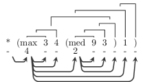
Figure 2: An example from the ListOps dataset. Numbers below operation tokens are valencies. (top) the original unlabelled phrase-structure. (bottom) our dependency conversion: each dependency represents either an operand to argument relation or a closing parenthesis relation.

	Acc.	Att.
Latent tree - ${\bm{G}}=0$
Forward relaxed	98.1	83.2
Straight-Through	70.8	33.9
Latent tree - MC training
Forward relaxed	99.6	99.7
Straight-Through	77.0	83.2

Table 1: ListOps results: tagging accuracy (Acc.) and attachment score for the latent tree grammar (Att.).

	Acc.	#Params
Yogatama et al. (2017)
*100D SPINN	80.5	2.3M
Maillard et al. (2017)
LSTM	81.2	161K
Latent Tree-LSTM	81.6	231K
Kim et al. (2017)
No Intra Attention	85.8	-
Simple Simple Att.	86.2	-
Structured Attention	86.8	-
Choi et al. (2018)
*100D ST Gumbel Tree	82.6	262K
300D ST Gumbel Tree	85.6	2.9M
600D ST Gumbel Tree	86.0	10.3M
Niculae et al. (2018)
Left-to-right Trees	81.0	-
Flat	81.7	-
Treebank	81.7	-
SparseMAP	81.9	-
Liu and Lapata (2018)
175D No Attention	85.3	600K
100D Projective Att.	86.8	1.2M
175D Non-projective Att.	86.9	1.1M
This work
No Intra Attention	84.4	382K
Simple Intra Att.	83.8	582K
Latent Tree + 1 GCN	85.2	703K
Latent Tree + 2 GCN	86.2	1M

Table 2: SNLI results and number of network parameters (discarding word embeddings). Stars indicate latent tree models.

Socher et al. (2013)
Bigram	83.1
Naive Bayes
Niculae et al. (2018)
CoreNLP	83.2
Latent tree	84.7
This work
CoreNLP	83.8
Latent tree	84.6

(a)

	Acc.
Williams et al. (2018a)
300D LSTM	69.1
300D SPINN	66.9
300D Balanced Trees	68.2
300D ST Gumbel Tree	69.5
300D RL-SPINN	67.3
This work
No Intra Attention	68.1
Latent tree + 1 GCN	71.5
Latent tree + 2 GCN	73.0

(b)

	Match	Mis.
Baselines
No Intra Att	68.5	68.9
Simple Intra Att	67.9	68.4
Left-to-right trees
1 GCN	71.2	71.8
2 GCN	72.3	71.1
Latent head selection model
1 GCN	69.0	69.4
2 GCN	68.7	69.6
Latent tree model
1 GCN	71.9	71.7
2 GCN	73.2	72.9

(c)

Table 3: LABEL:sub@tab:sst:results SST results. Stars indicate latent tree models. LABEL:sub@tab:multinli:results MultiNLI results. Stars indicate latent tree models. LABEL:sub@tab:ablation Ablation tests on MultiNLI (results on the matched and mismatched development sets).

6 Real-world Experiments

We evaluate our method on two real-world problems: a sentence comparison task (natural language inference, see Section 6.1) and a sentence classification problem (sentiment classification, see Section 6.2). Besides using the differentiable dynamic programming method, our approach also differs from previous work in that we use GCNs followed by a pooling operation, whereas most previous work used Tree-LSTMs. Unlike Tree-LSTMs, GCNs are trivial to parallelize over batches on GPU.

6.1 Natural Language Inference

The Natural Language Inference (NLI) problem is a task developed to test sentence understanding capacity. Given a premise sentence and a hypothesis sentence, the goal is to predict a relation between them: entailment, neutral or contradiction. We evaluate on the Stanford NLI (SNLI) and the Multi-genre NLI (MultiNLI) datasets. Our network is based on the decomposable attention (DA) model of Parikh et al. (2016). We induce structure of both the premise and the hypothesis (see Equation 1 and Figure 1b). Then, we run a GCN over the tree structures followed by inter-sentence attention. Finally, we apply max-pooling for each sentence and feed both sentence embeddings into a MLP to predict the label. Intuitively, using GCNs yields a form of intra-attention. See the hyper-parameters in Appendix A.2.

SNLI: The dataset contains almost 0.5m training instances extracted from image captions Bowman et al. (2015). We report results in Table 2.

Our model outperforms both no intra-attention and simple intra-attention baselines with 1 layer of GCN ($+0.8$) or two layers ($+1.8$). The improvements with using multiple GCN hops, here and on MultiNLI (Table 3b), suggest that higher-order information is beneficial. It is hard to compare different tree induction methods as they build on top of different baselines, however, it is clear that our model delivers results comparable with most accurate tree induction methods Kim et al. (2017); Liu and Lapata (2018). The improvements from using latent structure exceed these reported in previous work.

MultiNLI: MultiNLI is a broad-coverage NLI corpus Williams et al. (2018b): the sentence pairs originate from 5 different genres of written and spoken English. This dataset is particularly interesting because sentences are longer than in SNLI, making it more challenging for baseline models. We follow the evaluation setting in Williams et al. (2018b, a): we include the SNLI training data, use the matched development set for early stopping and evaluate on the matched test set. We use the same network and parameters as for SNLI. We report results in Table 3b.

The DA baseline (‘No Intra Attention’) performs slightly better ($+0.6\%$) than the original BiLSTM baseline. Our latent tree model significantly improves over our the baseline, either with a single layer GCN ($+3.4$%) or with a 2-layer GCN ($+4.9\%$). We observe a larger gap than on SNLI, which is expected given that MultiNLI is more complex. We perform extra ablation tests on MultiNLI in Section 6.3.

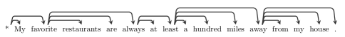
Figure 3: Examples of trees induced on the matched development set of MultiNLI, the model using 2 GCN layers.

6.2 Sentiment Classification

We experiment on the Stanford Sentiment Classification dataset Socher et al. (2013). The original dataset contains predicted constituency structure with manual sentiment labeling for each phrase. By definition, latent tree models cannot use the internal phrase annotation. We follow the setting of Niculae et al. (2018) and compare to them in two set-ups: (1) with syntactic dependency trees predicted by CoreNLP Manning et al. (2014); (2) with latent dependency trees. Results are reported in Table 3a.

First, we observe that the bag of bigrams baseline of Socher et al. (2013) achieves results comparable to all structured models. This suggest that the dataset may not be well suited for evaluating structure induction methods. Our latent dependency model slighty improves ($+0.8$) over the CoreNLP baseline. However, we observe that while our baseline is better than the one of Niculae et al. (2018), their latent tree model slightly outperforms ours ($+0.1$). We hypothesize that graph convolutions may not be optimal for this task.

6.3 Analysis

(Ablations) In order to test if the tree constraint is important, we do ablations on MultiNLI with two models: one with a latent projective tree variable (i.e. our full model) and one with a latent head selection model that does not impose any constraints on the structure. The estimation approach and the model are identical, except for the lack of the tree constraint (and hence dynamic programming) in the ablated model. We report results on development sets in Table 3c. We observe that the latent tree models outperform the alternatives.

Previous work (e.g., Niculae et al., 2018) included comparison with balanced trees, flat trees and left-to-right (or right-to-left) chains. Flat trees are pointless with the GCN + DA combination: the corresponding pooling operation is already done in DA. Though balanced trees are natural with bottom-up computation of TreeLSTMs, for GCNs they would result in embedding essentially random subsets of words. Consequently, we compare only to left-to-right chains of dependencies. This approach is substantially less accurate than our methods, especially for out-of-domain (i.e. mismatched) data.

(Grammar) We also investigate the structure of the induced grammar. We report the latent structure of three sentences in Figure 3. We observe that sentences are divided into spans, where each span is represented with a series of left dependencies. Surprisingly, the model chooses to use only left-to-right dependencies. The neural network does not include a RNN layer, so this may suggest that the grammar is trying to reproduce an recurrent model while also segmenting the sentence in phrases.

(Speed) We use a $\mathcal{O}(n^{3})$-time parsing algorithm. Nevertheless, our model is efficient: one epoch on SNLI takes 470 seconds, only 140 seconds longer than with the $\mathcal{O}(n^{2})$-time latent-head version of our model (roughly equivalent to classic self-attention). The latter model is computed on GPU (Titan X) while ours uses CPU (Xeon E5-2620) for the dynamic program and GPU for running the rest of the network.

7 Related work

Recently, there has been growing interest in providing an inductive bias in neural network by forcing layers to represent tree structures Kim et al. (2017); Maillard et al. (2017); Choi et al. (2018); Niculae et al. (2018); Williams et al. (2018a); Liu and Lapata (2018). Maillard et al. (2017) also operates on a chart but, rather than modeling discrete trees, uses a soft-gating approach to mix representations of constituents in each given cell. While these models showed consistent improvement over comparable baselines, they do not seem to explicitly capture syntactic or semantic structures Williams et al. (2018a). Nangia and Bowman (2018) introduced the ListOps task where the latent structure is essential to predict correctly the downstream prediction. Surprisingly, the models of Williams et al. (2018a) and Choi et al. (2018) failed. Much recent work in this context relies on latent variables, though we are not aware of any work closely related to ours. Differentiable structured layers in neural networks have been explored for semi-supervised parsing, for example by learning an auxiliary task on unlabelled data Peng et al. (2018) or using a variational autoencoder Corro and Titov (2019).

Besides research focused on inducing task-specific structures, another line of work, grammar induction, focused on unsupervised induction of linguistic structures. These methods typically rely on unlabeled texts and are evaluated by comparing the induced structures to actual syntactic annotation Klein and Manning (2005); Shen et al. (2018); Htut et al. (2018).

8 Conclusions

We introduced a novel approach to latent tree learning: a relaxed version of stochastic differentiable dynamic programming which allows for efficient sampling of projective dependency trees and enables end-to-end differentiation. We demonstrate effectiveness of our approach on both synthetic and real tasks. The analyses confirm importance of the tree constraint. Future work will investigate constituency structures and new neural architectures for latent structure incorporation.

Appendix A Neural Parametrization

(Implementation)

We implemented our neural networks with the C++ API of the Dynet library Neubig et al. (2017). The continuous relaxation of the parsing algorithm is implemented as a custom computation node.

(Training)

All networks are trained with Adam initialized with a learning rate of $0.0001$ and batches of size 64. If the dev score did not improve in the last 5 iterations, we multiply the learning rate by $0.9$ and load the best known model on dev. For the ListOps task, we run a maximum of 100 epochs, with exactly 100 updates per epoch. For NLI and SST tasks, we run a maximum of 200 epochs, with exactly 8500 and 100 updates per epoch, respectively.

All MLPs and GCNs have a dropout ratio of $0.2$ except for the ListOps task where there is no dropout. We clip the gradient if its norm exceed $5$.

A.1 ListOps Valency Tagging

(Dependency Parser)

Embeddings are of size 100. The BiLSTM is composed of two stacks (i.e. we first run a left-to-right and a right-to-left LSTM, then we concatenate their outputs and finally run a left-to-right and a right-to-left LSTM again) with one single hidden layer of size 100. The initial state of the LSTMs are fixed to zero.

The MLPs of the dotted attention have 2 layers of size 100 and a $\mathrm{ReLU}$ activation function

(Tagger)

The unique embedding is of size 100. The GCN has a single layer of size 100 and a $\mathrm{ReLU}$ activation. Then, the tagger is composed of a MLP with a layer of size 100 and a $\mathrm{ReLU}$ activation followed by a linear projection into the output space (i.e. no bias, no non-linearity).

A.2 Natural Language Inference

All activation functions are $\mathrm{ReLU}$. The inter-attention part and the classifier are exactly the same than in the model of Parikh et al. (2016).

(Embeddings)

Word embeddings of size 300 are initialized with Glove and are not updated during training. We initialize 100 unknown word embeddings where each value is sampled from the normal distribution. Unknown words are mapped using a hashing method.

(GCN)

The embeddings are first passed through a one layer MLP with an output size of 200. The dotted attention is computed by two MLP with two layers of size 200 each. Function $f()$, $g()$ and $h()$ in the GCN layers are one layer MLPs without activation function. The $\sigma$ activation function of a GCN is $\mathrm{ReLU}$. We use dense connections for the GCN.

A.3 Sentiment Classification

(Embeddings)

We use Glove embeddings of size 300. We learn the unknown word embeddings. Then, we compute context sensitive embeddings with a single-stack/single-layer BiLSTM with a hidden-layer of size 100.

(GCN)

The dotted attention is computed by two MLP with one layer of size 300 each. There is no distance bias in this model. Function $f()$, $g()$ and $h()$ in the GCN layers are one layer MLPs without activation function. The $\sigma$ activation function of a GCN is $\mathrm{ReLU}$. We do not use dense connections in this model.

(Output)

We use a max-pooling operation on the GCN outputs followed by an single-layer MLP of size 300.

Appendix B Illustration of the Continuous Relaxation

Too give an intuition of the continuous relaxation, we plot the $\operatorname*{arg\,max}$ function and the penalized $\operatorname*{arg\,max}$ in Figure 4. We plot the first output for input $(x_{1},x_{2},0)$.

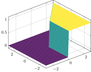
(a)

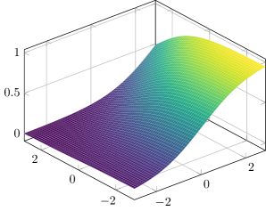
(b)

Figure 4: LABEL:sub@fig:argmax:a Single output of an $\operatorname*{arg\,max}$ function. The derivative is null almost everywhere, i.e. there is no descent direction. LABEL:sub@fig:argmax:b Single output of the differentiable relaxation. The derivatives are non-null.

Appendix C ListOps Training

We plot tagging accuracy and attachment score with respect to the training epoch in Figure 5. On the one hand, we observe that the non-stochastic versions converges way faster in both metrics: we suspect that it develops an alternative protocol to pass information about valencies from LSTM to the GCN. On the other hand, MC sampling may have a better exploration of the search space but it is slower to converge.

We stress that training with MC estimation results in the latent tree corresponding (almost) perfectly to the gold grammar.

Appendix D Fast differentiable dynamic program implementation

In order to speed up training, we build a a fast the differentiable dynamic program (DDP) as a custom computational node in Dynet and use it in a static graph. Instead of relying on masking, we add an input the DDP node that contains the sentence size : therefore, even if the size of the graph is fixed, the cubic-time algorithm is run on the true input length only. Moreover, instead of allocating memory with the standard library functionnality, we use the fast scratch memory allocator of Dynet.

(a)

(b)

Figure 5: Accuracy of tagging and attachment score of the latent tree during training. (red solid line) Non-stochastic training with forward relaxation. (blue dashed line) MC training with forward relaxation. (black dotted) Non-stochastic training with backward relaxation. (green dashdotted) MC with backward relaxation.

References

- Bastings et al. (2017) Joost Bastings, Ivan Titov, Wilker Aziz, Diego Marcheggiani, and Khalil Simaan. 2017. Graph convolutional encoders for syntax-aware neural machine translation. In Proceedings of the 2017 Conference on Empirical Methods in Natural Language Processing, pages 1947–1957. Association for Computational Linguistics.
- Bengio (2013) Yoshua Bengio. 2013. Estimating or propagating gradients through stochastic neurons. arXiv preprint arXiv:1305.2982.
- Bowman et al. (2015) Samuel R. Bowman, Gabor Angeli, Christopher Potts, and Christopher D. Manning. 2015. A large annotated corpus for learning natural language inference. In Proceedings of the 2015 Conference on Empirical Methods in Natural Language Processing, pages 632–642. Association for Computational Linguistics.
- Boyd and Vandenberghe (2004) Stephen Boyd and Lieven Vandenberghe. 2004. Convex optimization. Cambridge university press.
- Choi et al. (2018) Jihun Choi, Kang Min Yoo, and Sang-goo Lee. 2018. Learning to compose task-specific tree structures. In Proceedings of the 2018 Association for the Advancement of Artificial Intelligence (AAAI). and the 7th International Joint Conference on Natural Language Processing (ACL-IJCNLP).
- Corro and Titov (2019) Caio Corro and Ivan Titov. 2019. Differentiable perturb-and-parse: Semi-supervised parsing with a structured variational autoencoder. In Proceedings of the International Conference on Learning Representations.
- Cui et al. (2005) Hang Cui, Renxu Sun, Keya Li, Min-Yen Kan, and Tat-Seng Chua. 2005. Question answering passage retrieval using dependency relations. In Proceedings of the 28th annual international ACM SIGIR conference on Research and development in information retrieval, pages 400–407. ACM.
- Den Hertog et al. (1994) D Den Hertog, Cornelis Roos, and Tamás Terlaky. 1994. Inverse barrier methods for linear programming. RAIRO-Operations Research, 28(2):135–163.
- Eisner (1996) Jason M. Eisner. 1996. Three new probabilistic models for dependency parsing: An exploration. In COLING 1996 Volume 1: The 16th International Conference on Computational Linguistics.
- Foster et al. (2011) Jennifer Foster, Özlem Çetinoglu, Joachim Wagner, Joseph Le Roux, Stephen Hogan, Joakim Nivre, Deirdre Hogan, and Josef Van Genabith. 2011. # hardtoparse: Pos tagging and parsing the twitterverse. In AAAI 2011 workshop on analyzing microtext, pages 20–25.
- Fu (2006) Michael C Fu. 2006. Gradient estimation. Handbooks in operations research and management science, 13:575–616.
- Gould et al. (2016) Stephen Gould, Basura Fernando, Anoop Cherian, Peter Anderson, Rodrigo Santa Cruz, and Edison Guo. 2016. On differentiating parameterized argmin and argmax problems with application to bi-level optimization. arXiv preprint arXiv:1607.05447.
- Htut et al. (2018) Phu Mon Htut, Kyunghyun Cho, and Samuel Bowman. 2018. Grammar induction with neural language models: An unusual replication. In Proceedings of the 2018 Conference on Empirical Methods in Natural Language Processing, pages 4998–5003. Association for Computational Linguistics.
- Jang et al. (2017) Eric Jang, Shixiang Gu, and Ben Poole. 2017. Categorical reparameterization with gumbel-softmax. In Proceedings of the 2017 International Conference on Learning Representations.
- Kim et al. (2017) Yoon Kim, Carl Denton, Luong Hoang, and Alexander M Rush. 2017. Structured attention networks. In Proceedings of the International Conference on Learning Representations.
- Kingma and Welling (2014) Diederik P Kingma and Max Welling. 2014. Auto-encoding variational bayes. In Proceedings of the International Conference on Learning Representations.
- Kipf and Welling (2017) Thomas N Kipf and Max Welling. 2017. Semi-supervised classification with graph convolutional networks. In Proceedings of the International Conference on Learning Representations.
- Klein and Manning (2005) Dan Klein and Christopher D Manning. 2005. The unsupervised learning of natural language structure. Stanford University Stanford, CA.
- Lafferty et al. (2001) John Lafferty, Andrew McCallum, and Fernando CN Pereira. 2001. Conditional random fields: Probabilistic models for segmenting and labeling sequence data. In Proceedings of the 18th International Conference on Machine Learning.
- Liu and Lapata (2018) Yang Liu and Mirella Lapata. 2018. Learning structured text representations. Transactions of the Association for Computational Linguistics, 6:63–75.
- Liu et al. (2015) Yang Liu, Furu Wei, Sujian Li, Heng Ji, Ming Zhou, and Houfeng WANG. 2015. A dependency-based neural network for relation classification. In Proceedings of the 53rd Annual Meeting of the Association for Computational Linguistics and the 7th International Joint Conference on Natural Language Processing (Volume 2: Short Papers), pages 285–290. Association for Computational Linguistics.
- Maddison et al. (2014) Chris J Maddison, Daniel Tarlow, and Tom Minka. 2014. A* sampling. In Advances in Neural Information Processing Systems, pages 3086–3094.
- Maillard et al. (2017) Jean Maillard, Stephen Clark, and Dani Yogatama. 2017. Jointly learning sentence embeddings and syntax with unsupervised tree-LSTMs. arXiv preprint arXiv:1705.09189.
- Manning et al. (2014) Christopher Manning, Mihai Surdeanu, John Bauer, Jenny Finkel, Steven Bethard, and David McClosky. 2014. The stanford corenlp natural language processing toolkit. In Proceedings of 52nd Annual Meeting of the Association for Computational Linguistics: System Demonstrations, pages 55–60. Association for Computational Linguistics.
- Marcheggiani and Titov (2017) Diego Marcheggiani and Ivan Titov. 2017. Encoding sentences with graph convolutional networks for semantic role labeling. In Proceedings of the 2017 Conference on Empirical Methods in Natural Language Processing, pages 1507–1516. Association for Computational Linguistics.
- Mensch and Blondel (2018) Arthur Mensch and Mathieu Blondel. 2018. Differentiable dynamic programming for structured prediction and attention. In Proceedings of the 35th International Conference on Machine Learning.
- Nangia and Bowman (2018) Nikita Nangia and Samuel Bowman. 2018. Listops: A diagnostic dataset for latent tree learning. In Proceedings of the 2018 Conference of the North American Chapter of the Association for Computational Linguistics: Student Research Workshop, pages 92–99. Association for Computational Linguistics.
- Naradowsky et al. (2012) Jason Naradowsky, Sebastian Riedel, and David Smith. 2012. Improving NLP through marginalization of hidden syntactic structure. In Proceedings of the 2012 Joint Conference on Empirical Methods in Natural Language Processing and Computational Natural Language Learning, pages 810–820, Jeju Island, Korea. Association for Computational Linguistics.
- Neubig et al. (2017) Graham Neubig, Chris Dyer, Yoav Goldberg, Austin Matthews, Waleed Ammar, Antonios Anastasopoulos, Miguel Ballesteros, David Chiang, Daniel Clothiaux, Trevor Cohn, Kevin Duh, Manaal Faruqui, Cynthia Gan, Dan Garrette, Yangfeng Ji, Lingpeng Kong, Adhiguna Kuncoro, Gaurav Kumar, Chaitanya Malaviya, Paul Michel, Yusuke Oda, Matthew Richardson, Naomi Saphra, Swabha Swayamdipta, and Pengcheng Yin. 2017. Dynet: The dynamic neural network toolkit. arXiv preprint arXiv:1701.03980.
- Niculae et al. (2018) Vlad Niculae, André F. T. Martins, and Claire Cardie. 2018. Towards dynamic computation graphs via sparse latent structure. In Proceedings of the 2018 Conference on Empirical Methods in Natural Language Processing, pages 905–911. Association for Computational Linguistics.
- Papandreou and Yuille (2011) George Papandreou and Alan L Yuille. 2011. Perturb-and-MAP random fields: Using discrete optimization to learn and sample from energy models. In Computer Vision (ICCV), 2011 IEEE International Conference on, pages 193–200. IEEE.
- Parikh et al. (2016) Ankur Parikh, Oscar Täckström, Dipanjan Das, and Jakob Uszkoreit. 2016. A decomposable attention model for natural language inference. In Proceedings of the 2016 Conference on Empirical Methods in Natural Language Processing, pages 2249–2255. Association for Computational Linguistics.
- Peng et al. (2018) Hao Peng, Sam Thomson, and Noah A. Smith. 2018. Backpropagating through structured argmax using a spigot. In Proceedings of the 56th Annual Meeting of the Association for Computational Linguistics (Volume 1: Long Papers), pages 1863–1873. Association for Computational Linguistics.
- Petrov et al. (2010) Slav Petrov, Pi-Chuan Chang, Michael Ringgaard, and Hiyan Alshawi. 2010. Uptraining for accurate deterministic question parsing. In Proceedings of the 2010 Conference on Empirical Methods in Natural Language Processing, pages 705–713. Association for Computational Linguistics.
- Potra and Wright (2000) Florian A Potra and Stephen J Wright. 2000. Interior-point methods. Journal of Computational and Applied Mathematics, 124(1-2):281–302.
- Rangarajan (2000) Anand Rangarajan. 2000. Self-annealing and self-annihilation: unifying deterministic annealing and relaxation labeling. Pattern Recognition, 33(4):635–649.
- Schulman et al. (2015) John Schulman, Nicolas Heess, Theophane Weber, and Pieter Abbeel. 2015. Gradient estimation using stochastic computation graphs. In Advances in Neural Information Processing Systems, pages 3528–3536.
- Shen et al. (2018) Yikang Shen, Zhouhan Lin, Chin wei Huang, and Aaron Courville. 2018. Neural language modeling by jointly learning syntax and lexicon. In International Conference on Learning Representations.
- Socher et al. (2013) Richard Socher, Alex Perelygin, Jean Wu, Jason Chuang, Christopher D. Manning, Andrew Ng, and Christopher Potts. 2013. Recursive deep models for semantic compositionality over a sentiment treebank. In Proceedings of the 2013 Conference on Empirical Methods in Natural Language Processing, pages 1631–1642. Association for Computational Linguistics.
- Wang et al. (2018) Xinyi Wang, Hieu Pham, Pengcheng Yin, and Graham Neubig. 2018. A tree-based decoder for neural machine translation. In Proceedings of the 2018 Conference on Empirical Methods in Natural Language Processing, pages 4772–4777. Association for Computational Linguistics.
- Williams et al. (2018a) Adina Williams, Andrew Drozdov, and Samuel R. Bowman. 2018a. Do latent tree learning models identify meaningful structure in sentences? Transactions of the Association for Computational Linguistics, 6:253–267.
- Williams et al. (2018b) Adina Williams, Nikita Nangia, and Samuel Bowman. 2018b. A broad-coverage challenge corpus for sentence understanding through inference. In Proceedings of the 2018 Conference of the North American Chapter of the Association for Computational Linguistics: Human Language Technologies, Volume 1 (Long Papers), pages 1112–1122. Association for Computational Linguistics.
- Williams (1987) R Williams. 1987. A class of gradient-estimation algorithms for reinforcement learning in neural networks. In Proceedings of the International Conference on Neural Networks, pages II–601.
- Yogatama et al. (2017) Dani Yogatama, Phil Blunsom, Chris Dyer, Edward Grefenstette, and Wang Ling. 2017. Learning to compose words into sentences with reinforcement learning. In Proceedings of the International Conference on Learning Representations.