A low-rank method for time-dependent transport calculations

Abstract

Low-rank approximation is a technique to approximate a tensor or a matrix with a reduced rank to reduce the memory required and computational cost for simulation. Its broad applications include dimension reduction, signal processing, compression, and regression. In this work, a dynamical low-rank approximation method is developed for the time-dependent radiation transport equation in slab geometry. Using a finite volume discretization in space and Legendre polynomials in angle we construct a system that evolves on a low-rank manifold via an operator splitting approach. We demonstrate that the low-rank solution gives better accuracy than solving the full rank equations given the same amount of memory.

1 INTRODUCTION

We consider the transport of neutral particles as described by the linear Boltzmann equation,

$$\frac{1}{c}\frac{\partial\psi(z,\mu,t)}{\partial t}+\mu\frac{\partial\psi(z,\mu,t)}{\partial z}+\sigma_{\mathrm{t}}\psi(z,\mu,t)=\frac{\sigma_{\mathrm{s}}}{2}\int_{-1}^{1}\psi(z,\mu^{\prime},t)\,d\mu^{\prime}+S.$$ (1.1)

The total and isotropic scattering macroscopic cross-sections are denoted as $\sigma_{t}(z)$ and $\sigma_{s}(z)$, respectively, $c$ is the particle speed and $S(z,t)$ is a prescribed source. The angular flux $\psi(z,\mu,t)$ is a function of position $z$, time $t$, and the cosine of the polar angle $\mu\in[-1,1]$. We also write the scalar flux, $\phi(z,t)$, as the integral of the angular flux

$$\phi(z,t)=\int_{-1}^{1}\psi(z,\mu,t)\,d\mu.$$ (1.2)

In slab geometry we have a two-dimensional phase space and in principle there is a general function space that can describe solutions to the transport problem. Intuitively, it is known that many transport problems require only a subspace of this function space (called a manifold in mathematical parlance) to describe the transport. In other words, the solution is not any possible function of two variables, rather only a subset of functions. An example of this are problems in the diffusion limit: these problems require only a linear dependence on $\mu$. One can also formulate problems where this manifold over which the solution depends evolves over time: a beam entering a scattering medium would be described by a delta-function in space and angle at time zero, but eventually relax to much smoother distribution that we could characterize using a simple basis expansion.

We desire to generalize this idea, and possibly automatically discover the manifold that describes the system evolution. We accomplish this task by expressing the solution to a transport problem as a basis expansion in space and angle, and using techniques to determine what subspace of those bases are needed to describe the solution and how that subspace evolves. We use the dynamical low-rank approximation (DLRA) of Koch and Lubich to evolve time-dependent matrices by tangent-space projection [1]. DLRA has been extended to tensors [2] and further results can be found in [3]. DLRA has been used to reduce the computational complexity of quantum propagation [4] by restricting the evolution to lower-rank amongst other work [5, 6, 7, 8]. In this work, we apply DLRA to neutral particle transport.

Here we give a brief mathematical introduction of a robust and accurate projector-splitting method developed by Lubich [9] to perform the DLRA for matrix differential equations of the form

$$\frac{\partial}{\partial t}A(t)\equiv\dot{A}(t)=F(A(t)),$$

for $A(t)\in\mathbb{R}^{m\times n}$. DLRA seeks to find an approximating matrix $Y(t)$ of rank $r$ that minimizes the error in the Frobenius norm $||{Y}(t)-{A}(t)||_{\mathrm{f}}$. Then we note that rank $r$ matrices are a manifold, $\mathcal{M}_{r}$, of the space $\mathbb{R}^{m\times n}$. The solution to this minimization problem can be found using the singular value decomposition (SVD). However, to use the SVD this way we would need to have the solution $A(t)$.

We would prefer a way to evolve the solution on $\mathcal{M}_{r}$ directly. We reformulate the problem as minimizing the difference between the time derivative of the approximation and the solution $||\dot{Y}(t)-\dot{A}(t)||_{\mathrm{f}},$ where the derivative $\dot{Y}(t)$ is in the tangent space of $\mathcal{M}_{r}$. With a Galerkin condition the minimization problem is equivalent to an orthogonal projection. With the decomposition $Y(t)=U(t)S(t)V^{T}(t)$, this minimization problem can be solved using time splitting.

2 NUMERICAL METHOD

In this study we write the solution to Eq. (1.1) as

$$\psi(z,\mu,t)\approx\sum_{i,j=1}^{r}X_{i}(z,t)S_{ij}(t)W_{j}(\mu,t)$$ (2.1)

as the best approximation with rank $r$ of the solution for the equation (1.1), where we have written $X_{i}$ as an orthonormal basis for $z$ and $W_{j}$ as an orthonormal basis for $\mu$. We define the inner products

$$\langle f,g\rangle_{z}=\int_{0}^{Z}f(z)g(z)\,dz,\qquad\langle f,g\rangle_{\mu}=\int_{-1}^{1}f(\mu)g(\mu)\,d\mu.$$

Due to orthonormality we also have $\langle X_{i},{X}_{j}\rangle_{z}=\langle W_{i},{W}_{j}\rangle_{\mu}=\delta_{ij}.$ Then $\bar{X}=\{X_{1},X_{2},...,X_{r}\}$ and $\bar{W}=\{W_{1},W_{2},...,W_{r}\}$ are constructed as ansatz spaces. The expansion in Eq. (2.1) is not unique and we choose as gauge conditions $\langle X_{i},\dot{X}_{j}\rangle_{z}=0$ and $\langle W_{i},\dot{W}_{j}\rangle_{\mu}=0$. We now define orthogonal projectors using the bases:

$$P_{\bar{X}}g=\sum_{i=1}^{r}X_{i}\langle X_{i}g\rangle_{z}$$ (2.2)

$$P_{\bar{W}}g=\sum_{j=1}^{r}W_{j}\langle W_{j}g\rangle_{\mu}$$ (2.3)

We apply the projectors to define a split of the original equations into three steps and each of these is solved for a short time step

$$\partial_{t}\psi_{1}(z,\mu,t)=P_{\bar{W}}\left(-\mu\partial_{z}\psi_{1}(z,\mu,t)+\frac{\sigma_{\mathrm{s}}}{2}\int_{-1}^{1}\psi_{1}(z,\mu^{{}^{\prime}},t)\,d\mu^{{}^{\prime}}-\sigma_{t}\psi_{1}(z,\mu,t)+\frac{1}{2}S\right),$$ (2.4)

$$\partial_{t}\psi_{2}(z,\mu,t)=-P_{\bar{X}}P_{\bar{W}}\left(-\mu\partial_{z}\psi_{2}(z,\mu,t)+\frac{\sigma_{\mathrm{s}}}{2}\int_{-1}^{1}\psi_{2}(z,\mu,t)d\mu^{{}^{\prime}}-\sigma_{\mathrm{t}}\psi_{2}(z,\mu,t)+\frac{1}{2}S\right),$$ (2.5)

$$\partial_{t}\psi_{3}(z,\mu,t)=P_{\bar{X}}\left(-\mu\partial_{z}\psi_{3}(z,\mu,t)+\frac{\sigma_{\mathrm{s}}}{2}\int_{-1}^{1}\psi_{3}(z,\mu^{{}^{\prime}},t)d\mu^{{}^{\prime}}-\sigma_{\mathrm{t}}\psi_{3}(z,\mu,t)+\frac{1}{2}S\right).$$ (2.6)

The $\psi_{2}$ step uses $\psi_{1}$ as an initial condition, and the $\psi_{3}$ uses $\psi_{2}$ as an initial condition. It can be shown that the above evolution is contained in the low rank manifold $\mathcal{M}_{r}$, if the initial value is in $\mathcal{M}_{r}$ [9] because the right-hand side of each step remains in the tangent space $\mathcal{T}\mathcal{M}_{r}$.

To make the splitting more concrete we write $\psi_{1}$ as

$$\psi_{1}(z,\mu,t)=\sum_{j=1}^{r}K_{j}(z,t)W_{j}(\mu,t),$$ (2.7)

where $K_{j}(z,t)=\sum^{r}_{i}X_{i}(z,t)S_{ij}(t)$. We plug this solution into Eq. (2.4) and multiply by $W_{\ell}(\mu,t)$ and integrate over $\mu$ to get

$$\partial_{t}K_{j}+K_{j}\cancelto{0}{\langle W_{\ell}\dot{W}_{j}\rangle_{\mu}}=-\sum_{j^{\prime}=1}^{r}\langle\mu W_{j}W_{j^{\prime}}\rangle_{\mu}\partial_{z}K_{j^{\prime}}+\frac{\sigma_{\mathrm{s}}}{2}\sum_{j^{\prime}=1}g^{r}\langle W_{j}\rangle_{\mu}\langle W_{j^{\prime}}\rangle_{\mu}K_{j^{\prime}}-\sigma_{\mathrm{t}}K_{j}+\frac{\langle W_{j}\rangle_{\mu}}{2}S.$$ (2.8)

Notice that there is no change in $W_{j}$ bases in this equation. Equation (2.8) resembles the standard P_N equations, a point we will return to later. It is a system of advection problems in $z$.

We can then factorize $K_{j}$ into $X_{i}^{(1)}$ and $S_{ij}^{(1)}$. This is used to define an initial condition for $\psi_{2}=\sum_{i,j=1}^{r}X_{i}^{(1)}S_{ij}^{(1)}W_{j}.$ Then, we can perform similar calculations on Eq. (2.5) to get

$$\partial_{t}S_{ij}=\sum_{kl}^{r}\langle\partial_{z}X_{k}X_{i}\rangle_{z}S_{kl}\langle\mu W_{l}W_{j}\rangle_{\mu}-\frac{1}{2}\sum_{kl}^{r}\langle\sigma_{s}X_{k}X_{i}\rangle_{z}S_{kl}\langle W_{l}\rangle_{\mu}\langle W_{j}\rangle_{\mu}+\\ \sigma_{t}S_{ij}-\frac{1}{2}\langle X_{i}\rangle_{z}\langle W_{j}\rangle_{\mu}.$$ (2.9)

We call this solution $S_{ij}^{(2)}$. Equation (2.9) is a set of $r^{2}$ ordinary differential equations. The solution is used to create an initial condition for $\psi_{3}=\sum_{i,j=1}^{r}X_{i}^{(1)}S_{ij}^{(2)}W_{j}.$

Writing $L_{i}=S_{ij}(t)W_{j}(t,\mu)$ we can multiply Eq. (2.6) by a spatial basis function and integrate over space to get

$$\partial_{t}L_{i}=-\mu\sum_{k}^{r}\langle\partial_{z}X_{k}X_{i}\rangle_{z}L_{k}+\frac{1}{2}\langle\sigma_{s}X_{i}\rangle_{z}\langle L_{i}\rangle_{\mu}-\langle\sigma_{t}X_{i}\rangle_{z}L_{i}+\frac{1}{2}\langle X_{i}S\rangle_{z},$$ (2.10)

which evolves the solution in $\mu$ space. Upon factoring $L_{i}=S^{(3)}_{ij}(t)W_{j}^{(3)}(\mu,t)$, and write the solution as $\psi=\sum_{i,j,=1}^{r}X_{i}^{(1)}(x,t)S^{(3)}_{ij}(t)W_{j}^{(3)}(\mu,t).$

2.1 Discretization Details

The procedure outlined above of solving Eqs. (2.8), (2.9), and (2.10) in that order is accomplished by using a first-order explicit integration. The bases we use are based on a finite volume discretization in space with a constant mesh spacing $\Delta z$ and $m$ zones, and $n$ Legendre polynomials in angle. To make orthonormal bases we define

$$X_{i}(t,z)=\sum_{k=1}^{m}Z_{k}(z)u_{ki}(t)$$ (2.11)

$$W_{j}(t,\mu)=\sum_{l=1}^{n}P_{l}(\mu)v_{lj}(t)$$ (2.12)

Noted that $Z_{i}(z)=\frac{1}{\sqrt{\Delta z}}$ with $z\in[z_{i-\frac{1}{2}},z_{i+\frac{1}{2}}]$ where $i$ is the cell number, $P_{j}(\mu)=\sqrt{\frac{2n-1}{2}}\bar{P}_{n-1}(\mu)$, where $\bar{P}_{n}(\mu)$ is the $n_{th}$ order Legendre polynomial, $u_{ki}$ and $v_{lj}$ are components of the time dependent matrix $U(t)\in\mathbb{R}^{m\times r}$ and $V(t)\in\mathbb{R}^{n\times r}$. After the first and last step in the split the matrices $U$ and $V$ found by a QR decomposition to either $K_{j}$ or $L_{i}$.

The memory footprint required to compute the solution is the based on storing the matrices $U$, $V$ and $S$. Therefore, the memory required is

$$\mathrm{memory}=2(mr+r^{2}+nr),$$ (2.13)

the factor 2 assumes that we need to store the previous step solution as well as the new step. The full solution to this problem without splitting would require a memory footprint of $2mn$. Therefore, for $r\ll m,n$ there will be large memory savings.

In the solution procedure we needed to calculate $\langle\mu W_{j}W_{j^{\prime}}\rangle_{\mu}$. Using our angular basis this term becomes.

$$\langle\mu W_{j}W_{j^{\prime}}\rangle_{\mu}= \left\langle\mu\sum_{i=1}^{n}P_{i}(\mu)v_{ij}(t)\sum_{k=1}^{n}P_{k}(\mu)v_{kj^{\prime}}(t)\right\rangle_{\mu}=\left\langle\sum_{i=1}^{n}\sum_{k=1}^{n}v_{ij}(t)\mu P_{i}(\mu)P_{k}(\mu)v_{kj^{\prime}}(t)\right\rangle_{\mu}$$ (2.14)

$$= \sum_{i=1}^{n}\sum_{k=1}^{n}v_{il}(t)\langle\mu P_{i}(\mu)P_{k}(\mu)\rangle_{\mu}v_{kj}(t)$$

Note that $\langle\mu P_{i}(\mu)P_{k}(\mu)\rangle_{\mu}$ forms a $n\times n$ matrix, $C$, that can be precomputed. Thus Eqs. (2.14) requires $\mathcal{O}(n^{2}r)$ operations, which is affordable because usually $n$ is not large and $C$ is sparse. Alternatively, we could calculate $\langle\mu W_{j}W_{j^{\prime}}\rangle_{\mu}$ on-the-fly by choosing $\mathcal{O}(n)$ quadrature points in angle, and it requires $\mathcal{O}(nr^{2})$ operations for all the $r^{2}$ entries.

Additionally, using the standard upwinding technique for the spatial derivative terms leads to

$$\partial_{z}K\langle\mu W^{T}W\rangle_{\mu}= \frac{1}{\sqrt{\Delta z}}(K_{i+\frac{1}{2}}-K_{i-\frac{1}{2}})\langle\mu W^{T}W\rangle_{\mu}$$ (2.15)

$$=\frac{1}{2\sqrt{\Delta z}}[(K_{i+1}-K_{i-1})V^{T}CV-(K_{i+1}-2K_{i}+K_{i-1})V^{T}\Sigma V],$$ (2.16)

where $\Sigma$ is a stabilization matrix that we take to be a diagonal matrix with the singular values of $C$. Other stabilization terms could be used, including Lax-Friedrichs where $V^{T}\Sigma V$ is replaced by a constant times an identity matrix.

The spherical harmonic we used in the angular expansion can yield oscillatory or negative solutions. To address this issue we implemented angular filtering [10, 11] which can significantly increase the performance of $P_{n}$ method in solving radiative transfer equation by removing the oscillations. We implemented the filter into our explicit solver and combined it with the low-rank approximation algorithm. The filtered equation adds anisotropic scattering. In this study we use a Lanczos filter.

2.2 Conservation

The low-rank algorithm we have described does not conserve the number of particles. This loss of conservation is a result of information lost in the algorithm when restricting the solution to low rank descriptions. We have addressed this by globally scaling the solution after each time step to correct for any particles lost. This point is discussed in further detail in the conclusion section.

3 NUMERICAL RESULTS

3.1 Plane source problem

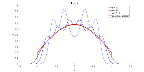
(a) Low-rank solutions without a filter

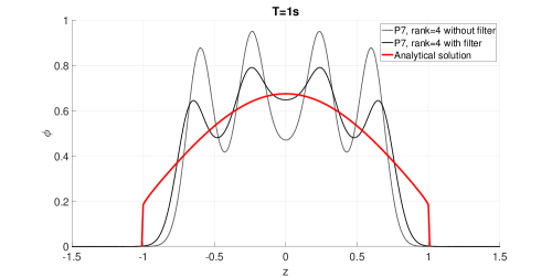
(b) Comparison of P₇ solutions of rank $4$ with and without a filter.

Figure 3.1: Solutions to the plane source problem using the low rank method compared to the analytic solution.

First, we solve the plane source problem of a delta function source in space and time in a purely scattering medium with $\sigma_{\mathrm{t}}=\sigma_{\mathrm{s}}=1$; the analytical benchmark solution was given by Ganapol [12]. For this problem we fix the spatial resolution to be $\Delta z=0.01$ (this corresponds to $m=301$ for the $t=1$ solution and $m=1201$ for the $t=5$ results), and vary the number of angular basis functions, $n$, and the rank $r$. When used, the filter strength is set to $50$.

Figure 3.1 shows the solutions of varying rank and Legendre polynomial orders with and without a filter. We can see the low-rank solution using a P₁₅ basis matches the analytic solution to the scale of the graph in the middle of the problem. We also observe that the low-rank solution can be improved by the filter: P₇ solutions of reduced rank improve when a filter is used.

For a more quantitative comparison, the error of the numerical results with different $n$ and $r$ is shown in Figure 3.2. In this figure the colors for the dotted lines correspond to the rank used in a calculation and different values of the $n$, the number of angular basis functions, are corresponding dots. For each color the value of $n$ ranges from $r$ to $100$. The large points are the value of the error using the standard full rank method with $r=n$. We can observe that the low-rank solution is more accurate than the full rank with the same memory usage. For example, the error of full rank solution $n=12$ using with a memory footprint of $8000$ is about $0.07$. With less memory, the error can be reduced to $0.02$. We can also use $70\%$ of the memory to achieve the same accuracy. Increasing the resolution and rank will contribute to the accuracy of solutions. Given the way we performed this study with a fixed spatial mesh and time step and the conservation fix we used, we can see some error stagnation in the low-rank solution at $t=5$. Other numerical experiments indicate that increasing the number of spatial zones can further decrease the error.

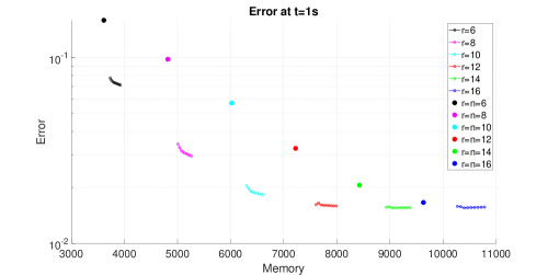
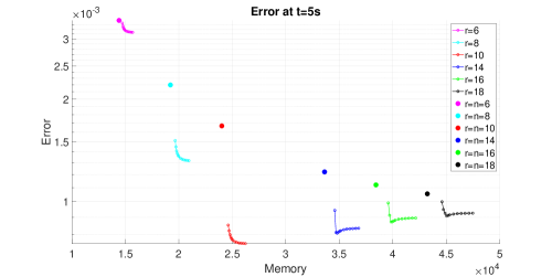
Figure 3.2: The comparison of errors on the plane source problem with different memory usage are shown. Each dotted line represents the error with a fixed rank that varies the number of angular basis functions $n$. The bold dot denotes the full rank solution.

3.2 Reed’s problem

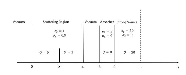
Figure 3.3: The material layout in Reed’s problem.

The second problem is Reed’s problem [13, 14, 15], which is a multi-material problem, and its set-up is detailed in Fig. 3.3. Because Reed’s problem does not have an analytical solution, a numerical result with high resolution and full rank, where $\Delta z=0.01$ ($m=1600$), P₉₉ ($n=100$) and $CFL=\Delta t/\Delta x=0.1$, is set as a benchmark for memory analysis. It can be observed in Figure 3.4 that the low rank solutions (solid lines with small dots) can give solutions with comparable errors to the full rank solutions (large dots) with much larger memory. For example the rank $8$ solutions obtain a solution error better than the full rank $P_{19}$ solution with less memory.

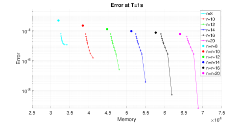
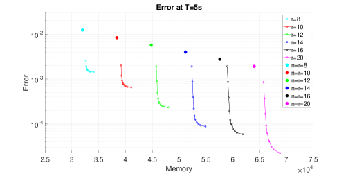
Figure 3.4: The comparison of errors for Reed’s problem with different memory usage are shown. Each dotted line represents the error with a fixed rank that varies the number of angular basis functions $n$. The bold dot denotes the full rank solution.

4 CONCLUSIONS

We have developed a practical algorithm to find the low-rank solution of the slab geometry transport equation using explicit time integration. The method is based on projecting the equation to low-rank manifolds and numerically integrating in three steps. The numerical simulations show that on several test problems the memory savings of the low-rank method can be on the order of a factor of 2-3. Given that these are only slab geometry problems we expect even larger memory savings on 2- and 3-D problems due to their larger size. Exploring this is ongoing work. Furthermore, we will be investigating other means for correcting the loss of conservation in the method, including posing the problem as a high-order/low-order problem.

References

- [1] O. Koch and C. Lubich. “Dynamical low-rank approximation.” SIAM Journal on Matrix Analysis and Applications, volume 29(2), pp. 434–454 (2007).
- [2] O. Koch and C. Lubich. “Dynamical Tensor Approximation.” SIAM Journal on Matrix Analysis and Applications, volume 31(5), pp. 2360–2375 (2010).
- [3] A. Nonnenmacher and C. Lubich. “Dynamical low-rank approximation: applications and numerical experiments.” Mathematics and Computers in Simulation, volume 79(4), pp. 1346–1357 (2008).
- [4] B. Kloss, I. Burghardt, and C. Lubich. “Implementation of a novel projector-splitting integrator for the multi-configurational time-dependent Hartree approach.” Journal of Chemical Physics, volume 146(17) (2017). URL https://doi.org/10.1063/1.4982065.
- [5] T. Jahnke and W. Huisinga. “A dynamical low-rank approach to the chemical master equation.” Bulletin of Mathematical Biology, volume 70(8), pp. 2283–2302 (2008).
- [6] T. Boiveau, V. Ehrlacher, A. Ern, and A. Nouy. “Low-rank approximation of linear parabolic equations by space-time tensor Galerkin methods.” (arXiv:1712.07256v1) (2017). URL https://arxiv.org/pdf/1712.07256.pdf.
- [7] L. Einkemmer and C. Lubich. “A low-rank projector-splitting integrator for the Vlasov–Poisson equation.” SIAM Journal on Scientific Computing, pp. 1–23 (2018). URL http://arxiv.org/abs/1801.01103.
- [8] I. Markovsky. “Structured low-rank approximation and its applications.” Automatica, volume 44(4), pp. 891–909 (2008).
- [9] C. Lubich and I. V. Oseledets. “A projector-splitting integrator for dynamical low-rank approximation.” BIT Numerical Mathematics, volume 54(1), pp. 171–188 (2014).
- [10] R. G. McClarren and C. D. Hauck. “Robust and accurate filtered spherical harmonics expansions for radiative transfer.” Journal of Computational Physics, volume 229(16), pp. 5597–5614 (2010).
- [11] D. Radice, E. Abdikamalov, L. Rezzolla, and C. D. Ott. “A new spherical harmonics scheme for multi-dimensional radiation transport I. Static matter configurations.” Journal of Computational Physics, volume 242, pp. 648–669 (2013).
- [12] B. Ganapol. Analytical Benchmarks for Nuclear Engineering Applications. Organisation for Economic Co-Operation and Development (2008).
- [13] W. Reed. “New difference schemes for the neutron transport equation.” Nucl Sci Eng, volume 46, pp. 31–39 (1971).
- [14] R. G. McClarren. Spherical harmonics methods for thermal radiation transport. Ph.D. thesis, University of Michigan (2007).
- [15] W. Zheng and R. G. McClarren. “Moment closures based on minimizing the residual of the PN angular expansion in radiation transport.” Journal of Computational Physics, volume 314, pp. 682–699 (2016).