Dynamic Network Embeddings for Network Evolution Analysis

Abstract.

Network embeddings learn to represent nodes as low-dimensional vectors to preserve the proximity between nodes and communities of the network for network analysis. The temporal edges (e.g., relationships, contacts, and emails) in dynamic networks are important for network evolution analysis, but few existing methods in network embeddings can capture the dynamic information from temporal edges. In this paper, we propose a novel dynamic network embedding method to analyze evolution patterns of dynamic networks effectively. Our method uses random walk to keep the proximity between nodes and applies dynamic Bernoulli embeddings to train discrete-time network embeddings in the same vector space without alignments to preserve the temporal continuity of stable nodes. We compare our method with several state-of-the-art methods by link prediction and evolving node detection, and the experiments demonstrate that our method generally has better performance in these tasks. Our method is further verified by two real-world dynamic networks via detecting evolving nodes and visualizing their temporal trajectories in the embedded space.

1. INTRODUCTION

Networks describe the relationships between entities, such as social relationships within a population, interactions between biological proteins, and co-occurrence relationships within words. Dynamic networks are very common in many application domains with entities and connections changing over time, such as email networks and instant messaging networks. Analyzing these networks can gain insight into evolution patterns in these domains. Recently, dynamic network analysis has received much attention, and many embedding-based approaches have been proposed for temporal link prediction (Nguyen et al., 2018), node prediction (Zhou et al., 2018), and multi-label node classification (Ma et al., 2018). Thus, utilizing embeddings to investigate network evolution is a promising research direction.

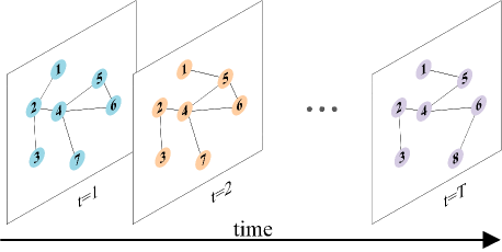
Figure 1. An illustration of a social network with the addition and deletion of nodes and edges over time. For example, node 7 disappears at $t=T$, and node 8 appears at $t=T$. The edge between node 1 and node 2 is deleted at $t=2$, and a new connection between node 1 and node 5 is generated.

As illustrated in Figure 1, a social network is evolving with the addition and deletion of nodes and edges over time. Each node represents a person, and each edge indicates one kind of events between two persons, such as friendship, contacts, and emails. The weight of an edge denotes how strong this relationship is or the frequency of communication (e.g., the number of emails or calls). Two most important factors in dynamic networks are the proximity between nodes and temporal continuity of stable nodes along the time, which should be preserved in network embeddings for effective network evolution analysis. For instance, node 1 and node 3 share the same neighbor nodes at $t=1$ in Figure 1, but this relation is decreased at $t=2$ (i.e., proximity similarity). The neighbor nodes of node 4 at $t=1$ and $t=2$ are similar. Thus, the embedded vectors of node 4 at the two timesteps should be nearly the same (i.e., temporal similarity).

Previous methods for network embeddings, such as matrix factorization (Cao et al., 2015), random walk (Perozzi et al., 2014; Grover and Leskovec, 2016; Ribeiro et al., 2017), deep neural network (Cao et al., 2016; Wang et al., 2016; Ni et al., 2018; Dai et al., 2018), and many others (Tang et al., 2015; Gu et al., 2018), generally focus on static networks to preserve the proximity between nodes. These methods fail to capture the temporal information in dynamic networks. Recently, continuous-time dynamic network embeddings (Nguyen et al., 2018) aim to learn continuous changes in temporal networks by temporal walk, which is a walking strategy with a time-ascending order. However, this method represents all network information into one embedding and cannot effectively capture the temporal changes of nodes over time, such as evolving node detection. DynamicTriad (Zhou et al., 2018) seeks to train all graphs in a dynamic network jointly into a sequence of embeddings by imposing triad. However, the triad, a local proximity, only describes the local relation among up to three nodes, and can hardly capture high-order proximities between nodes.

In this paper, we attempt to learn discrete-time network embeddings for dynamic network, i.e., each node has the same number of low-dimensional vectors with the number of timesteps and both the proximity and temporal continuity of each node are preserved in the dynamic network embeddings. A direct method to solve this problem is to learn each graph separately by static network embedding methods, and then align all network embeddings into the same vector space by alignment methods (Hamilton et al., 2016). However, it is challenging to align these embeddings due to nonlinear movements of evolving nodes, and such alignment error would reduce the performance of downstream tasks. Thus, we propose a novel dynamic network embedding method to learn a sequence of graphs in a dynamic network and generate continuous embedded vectors for stable nodes without embedding alignments. Dynamic network embeddings can capture neighbor node changes over time for evolution analysis. Generally, this paper has the following contributions:

• We propose a general dynamic network embedding method that incorporates random walk on dynamic networks into Bernoulli embeddings.

• Our method is more effective in link prediction when compared with other state-of-the-art techniques. Besides, we generate artificial dynamic networks to verify our method in capturing the temporal evolution of nodes and achieve the best performance.

• Our method can be used to analyze and visualize the trajectories of evolving nodes while preserving the temporal continuity of stable nodes over time.

2. RELATED WORK

With the rise of social networks (e.g., Facebook and Twitter) and big data (e.g., millions or billions of interaction records), network embedding methods have received considerable attention from both industrial and academic. The key point of network embeddings is to learn a low-dimensional vector representation for each node to preserve the proximity, which can be easily used for several application tasks, for instance, node classification (Perozzi et al., 2014), link prediction (Ou et al., 2016), node clustering (Wang et al., 2017), anomaly detection (Hu et al., 2016), and collaboration prediction (Chen and Sun, 2017).

Some network embedding methods are based on matrix factorization (Cao et al., 2015), which constructs a $k$-step transition probability matrix to measure the node similarity at different scales. Inspired by a good performance of word2vec in natural language processing, some researchers incorporated random walk into the skip-gram model (Mikolov et al., 2013a) to learn network embeddings, such as DeepWalk (Perozzi et al., 2014) and node2vec (Grover and Leskovec, 2016). These methods use random walk to produce a series of node sequences and apply the skip-gram model to learn network representations. Struc2vec (Ribeiro et al., 2017) focuses on the structural identities of nodes and constructs a weighted multilayer graph for random walk to capture the hierarchical structural similarity. Recently, some embedding methods based on deep neural networks have received considerable attention (Wang et al., 2016; Cao et al., 2016; Ni et al., 2018) to learn nonlinear mapping functions. To enhance the robustness of representations, Dai et al. employed generative adversarial network to capture latent features in network embeddings (Dai et al., 2018).

Most previous network embedding methods only focus on static networks, but dynamic network embedding learning is a hot research topic. It is related to dynamic latent space models, such as a dynamic model accounting for friendships drifting over time (Sarkar and Moore, 2006) and a case-control approximate likelihood (Raftery et al., 2012). CTDNE (Nguyen et al., 2018) incorporates temporal information into existing network embedding methods based on random walk by introducing a time-series order. TNE (Zhu et al., 2016) is a discrete-time dynamic network embedding method based on matrix factorization. DynGEM (Kamra et al., 2017) is based on deep autoencoders combined with a layer expansion to generate embeddings of a growing network. DynamicTriad (Zhou et al., 2018) focuses on the local structure called triad to learn the proximity information and evolution patterns. TIMERS (Zhang et al., 2018) uses a SVD model to learn dynamic network embeddings incrementally based on the initialization of the previous graph. DepthLGP (Ma et al., 2018) tackles the issue of updating out-of-sample nodes into network embeddings by combining a probabilistic model with deep learning. Previous methods evaluate network embeddings only by static tasks, and the trajectories of evolving nodes have not received much attention. Therefore, one of our evaluations is evolving node detection, and we further visualize the trajectories of evolving nodes in the context of stable nodes for evolution pattern analysis.

3. PROBLEM DEFINITION

In this paper, we seek to solve the proximity and temporal representation problem of dynamic networks, i.e., each node has one embedded vector in each timestep. Recently, the exploration of word meaning evolution in natural language processing has received much attention, and the key is to understand how words change their meanings over time and mine the latent cultural evolution (Kutuzov et al., 2018). Kulkarni et al. proposed an insightful conception of aligning all word embeddings at different timesteps into one vector space before semantic shift analysis (Kulkarni et al., 2015). Instead of a linear transformation for the alignment, Eger and Mehler presented second-order embeddings to compare the difference of word meanings (Eger and Mehler, 2017). Moreover, it was shown in (Bamler and Mandt, 2017) and (Yao et al., 2018) that we can learn diachronic word embeddings in the same vector space jointly. Thus the alignment across of embeddings is simultaneous and accurate.

Inspired by these diachronic word embeddings, we propose a novel method to generate embeddings for dynamic networks. The definition of dynamic networks is given as follows:

Definition 3.1 (Dynamic Networks).

A dynamic network is a series of graphs $\Gamma=\{G_{1},...,G_{T}\}$ and $G_{t}=(V_{t},E_{t})$, where $T$ is the number of graphs, $V_{t}$ is a node set and $E_{t}$ includes all temporal edges within the timespan $[S_{t},S_{t+1}]$. Each $e_{i}=(u,v,s_{i})\in E_{t}$ is a temporal edge between the node $u\in V_{t}$ and the node $v\in V_{t}$ at the timestamp $s_{i}\in[S_{t},S_{t+1}]$.

A dynamic network can be constructed from temporal events, and different construction methods may have different applications, as discussed in Section 4.1. Our goal is to learn dynamic network embeddings $M_{1},...,M_{T}$ and $M_{t}\in\mathbb{R}^{|V_{t}|\times D}$, where $|V_{t}|$ is the number of nodes at timestep $t$ and $D$ is the dimension of embeddings. Thus, the concept of dynamic network embeddings is defined formally as follows:

Definition 3.2 (Dynamic Network Embeddings).

Given a dynamic network $\Gamma=\{G_{1},...,G_{T}\}$, dynamic network embeddings aim to project a node $g\in V_{t}$ into a low-dimensional vector space by a mapping function $\textit{f}:g\mapsto y_{g}^{(t)}\in\mathbb{R}^{D},D\ll\max|V_{t}|,t\in[1,T]$.

Thus, there is an embedding matrix $M_{t}\in\mathbb{R}^{|V_{t}|\times D}$ to represent the proximity and temporal properties for each graph $G_{t}$. The dynamic network embeddings generally require the following characteristics:

• Proximity Preservation. The embeddings should preserve the proximity between nodes, i.e., if a node $u$ and a node $v$ have similar neighbor nodes at timestep $t$, $y_{u}^{(t)}$ and $y_{v}^{(t)}$ should be located nearby in the vector space.

• Temporal Continuity. The embeddings should keep the temporal similarity of stable nodes, i.e., if a node $u$ has similar neighbors at timestep $t$ and $t+1$, $y_{u}^{(t)}$ and $y_{u}^{(t+1)}$ should be located nearby in the vector space.

• Dimension Reduction. Although dynamic networks can be complex with thousands of nodes and temporal edges, the embeddings should be low-dimensional, i.e., $D\ll max|V_{t}|$. Therefore, the embeddings can be effectively applied to downstream machine learning tasks.

4. PROPOSED METHOD

Our method has three main steps. Firstly, we construct a dynamic network from temporal events. Then we apply random walk to generate node sequences matrix for each graph to keep the local proximity for each node in each timestep. Finally, we learn node representations from all node sequences of all timesteps jointly based on Bernoulli embeddings, as shown in Algorithm 1.

4.1. Dynamic Network Construction

The relationships between entities are generally described by timestamped events in real-world datasets, such as emails, calls, and interaction records. We first need to transform these temporal events into a dynamic network by constructing a sequence of graphs before learning its dynamic network embeddings.

One strategy is the fixed time interval $\omega$ (e.g., hours, days, and weeks) for each timestep. Thus, each graph $G_{t}$ has a time window $[S_{t},S_{t}+\omega)$ and $S_{t}$ is the earliest timestamp of timestep $t$. The temporal edge set of timestep $t$ is

(1) $$E_{t}=\{e_{i}|s_{i}\in[S_{t},S_{t}+\omega)\}.$$

Since the events may be not evenly distributed over time, graphs would have different numbers of events. For example, one graph may contain one thousand temporal edges, while the other graph may only have one hundred temporal edges. The dynamic network embeddings learned from these graphs with non-uniform events may have a negative impact on downstream tasks, especially for sparse graphs. Thus, it would be better to choose different time intervals for different timesteps, and construct a dynamic network by a fixed number of events $\varepsilon$ (the other strategy). The events can be generally described as follows (the number of events is $N$):

(2) $$A=(e_{1},e_{2},...e_{N}).$$

Each graph $G_{t}$ has an event window $(\varepsilon\cdot(t-1),\varepsilon\cdot t]\subset[1,N]$ , and the edge set of timestep $t$ is defined as follows:

(3) $$E_{t}=\{e_{i}|i\in(\varepsilon\cdot(t-1),\varepsilon\cdot t]\}.$$

In this way, each graph has nearly the same number of events. However, the drawback is breaking the equivalent time interval, which may be important for some applications. We can select the fixed time interval or the fixed number of events depending on tasks when constructing dynamic networks.

Figure 2. Dynamic network construction by the fixed time interval or the fixed number of events.

The hard boundary may generate discontinuous network embeddings over time and lead to misleading evolution patterns. To address this issue, the window of each graph has an overlap $\gamma\in[0,1]$ with the previous graph, as shown in Figure 2. For the fixed time interval, the time window $\omega>\Delta t$ (non-overlapping time interval) and the overlap $\gamma$ is defined as $\gamma=(\omega-\Delta t)/\omega$. For the fixed number of events, the event window $\varepsilon>\Delta e$ (non-overlapping events) and the overlap $\gamma$ is defined as $\gamma=(\varepsilon-\Delta e)/\varepsilon$. In our experiment, we choose to adjust $\varepsilon$ for the link prediction and evolving node detection tasks, and adjust $\omega$ for analyzing and visualizing the trajectories of evolving nodes.

Algorithm 1 Dynamic Network Embeddings

0:  A dynamic networks $\Gamma=\{G_{1},...,G_{T}\},G_{t}=(V_{t},E_{t})$number of walks on each node $r$length of each walk $L$embedding size $D$context size $cs$negative sample size $ns$

0:  Network embeddings $M_{1},...,M_{T}$Initialize embedding matrix $M_{1},...,M_{T}$Initialize context matrix $\alpha$

  for $t=1$ to $T$ do

     for each $g\in V_{t}$ do

        $W_{g}^{(t)}=RandomWalk(G_{t},g,r,L)$

        DBE($y_{g}^{(t)}$,$\alpha_{g}$,$W_{g}^{(t)}$,$V_{t}$,$cs$,$ns$)

     end for

  end for

4.2. Sequential Random Walks

We use random walk to capture the proximity information of each graph and generate sequences of walks as the input for network embeddings learning. For each graph, we first choose a node as the root of a random walk, then the walk selects uniformly from the neighbors of the last node visited until the maximum length $L$ of a node sequence is reached. The walking process will repeat $r$ times for each node of each graph. Instead of repeating the walking process in each graph iteratively, our approach runs random walk on graphs parallelly to generate one node sequence matrix $W_{t}$ for each graph $G_{t}$. In natural language processing, the context is composed of the words appearing to both the right and left of the given word. For the network, the context means the neighbors of the node, and the nodes before and after the node in the node sequence are the context of the node.

4.3. Dynamic Bernoulli Embeddings

We introduce the dynamic Bernoulli embedding method for latent representation learning of a dynamic networks (Algorithm 2). A node sequence $w_{j}^{(t)}=\{v_{1}^{(t)},...,v_{L}^{(t)}\}$ is generated from the node $j$ at timestep $t$ by random walk. We define the context of $v_{i}^{(t)}$ in the node sequence as $c_{i}^{(t)}=\{v_{i-cs/2}^{(t)},...,v_{i+cs/2}^{(t)}\}\setminus v_{i}^{(t)}$, where the context size is $cs$. $x_{i}^{(t)}\in\mathbb{R}^{|V_{t}|}$ is an indicator vector that each entry $x_{ig}$ is zero or one, and $x_{ig}^{(t)}=1$ means $v_{i}^{(t)}$ is the node $g$.

We assign $x_{ig}^{(t)}$ with a conditional distribution $P(x_{ig}^{(t)}|c_{i}^{(t)})$ based on a Bernoulli probability. Likewise, we define $\alpha_{g}\in\mathbb{R}^{D}$ as the context for the node $g$ and we update it in the process of dynamic embedding learning at each timestep. In contrast, we only update the embedding vector $y_{g}^{(t)}$ of $M_{t}$ when we train the node $v_{i}^{(t)}$ at timestep $t$. Finally, we define the representation function of $g$ and $c_{i}^{(t)}$ at timestep $t$ as follows:

(4) $$\eta_{ig}=y_{g}^{(t)T}(\sum_{\begin{subarray}{c}k\neq i\\ k\in[i-cs/2,i+cs/2]\end{subarray}}\sum_{g\in V_{t}}\alpha_{g}x_{k{g}}^{(t)}),$$

where the sum $\sum_{g}\alpha_{g}x_{kg}^{(t)}$ is a filter to select the context vector $\alpha_{g}$. With the shared context vector $\alpha_{g}$ for all timesteps, we can train all embeddings in the same vector space and capture the evolution information across all timesteps.

To initialize embeddings $M_{1},...,M_{T}$ and $\alpha$, we use Gaussian priors with a diagonal covariance, and set parameters $\lambda_{1}$ and $\lambda$ according to (Rudolph and Blei, 2018).

(5) $$\alpha_{g},y_{g}^{(1)} \sim N(0,\lambda_{1}^{-1}I)$$

(6) $$y_{g}^{(t)} \sim N(y_{g}^{(t-1)},\lambda^{-1}I).$$

To achieve better performance, we can use embeddings pretrained by static methods as the default value of $M_{t}$ to speed up the convergence of our model.

To train dynamic network embeddings, we regularize the pseudo log likelihood with the log priors, and then maximize the likelihood to obtain a pseudo MAP estimation. Furthermore, we consider the contributions of positive context nodes and negative context nodes separately, and we define these two likelihoods $\mathcal{L}_{pos}$ and $\mathcal{L}_{neg}$ as follow:

(7) $$\mathcal{L}_{pos} =\sum_{i=1}^{L}\sum_{g\in{V_{t}}}x_{ig}^{(t)}\log\sigma(\eta_{ig}),$$

(8) $$\ \mathcal{L}_{neg} =\sum_{i=1}^{L}\sum_{g\in{V_{t}}}(1-x_{ig}^{(t)})\log(1-\sigma(\eta_{ig})),$$

where $\sigma(\cdot)$ is the sigmoid function to generate the probability. Considering negative context nodes are far more than positive context nodes, we use negative sampling to randomly select nodes except node $g$ as negative context nodes to reduce the computation of $\mathcal{L}_{neg}$. We define the sampling distribution of negative context nodes is $\phi$, and Equation 8 is redefined as:

(9) $$\ \mathcal{L}_{neg}=\sum_{i=1}^{L}\sum_{g\sim\phi}\log(1-\sigma(\eta_{ig})).$$

In this paper, we set the unigram distribution (Mikolov et al., 2013b) raised to the power of 0.75 as $\phi$. We notice that $y$ and $\alpha$ are the terms of Equation 4 which is included in Equation 7 and 9. Thus, we set a prior to $\alpha$:

(10) $$\mathcal{L}_{\alpha}=-\frac{\lambda_{1}}{2}\sum_{g\in{V_{t}}}\|\alpha_{g}\|^{2}.$$

To penalize the consecutive embedding vector $y_{g}^{(t-1)}$ and $y_{g}^{(t)}$ for drifting from each too far apart, we set the prior of $y$ as:

(11) $$\mathcal{L}_{y}=-\frac{\lambda_{1}}{2}\sum_{g\in{V_{t}}}\|y_{g}^{(1)}\|^{2}-\frac{\lambda}{2}\sum_{\begin{subarray}{c}g\in{V_{t}}\\ t\in[1,T]\end{subarray}}\|y_{g}^{(t)}-y_{g}^{(t-1)}\|^{2}.$$

Finally, we group all likelihoods as the optimization objective:

(12) $$\mathcal{L}(y,\alpha)=\mathcal{L}_{pos}+\mathcal{L}_{neg}+\mathcal{L}_{\alpha}+\mathcal{L}_{y}.$$

Overall, we use Stochastic Gradient Descent (SGD) (Robbins and Monro, 1985) to fit Equation 12 with a proper learning rate.

Algorithm 2 DBE($y_{g}^{(t)}$,$\alpha_{g}$,$W_{g}^{(t)}$,$V_{t}$,$cs$,$ns$)

  for each $w_{k}^{(t)}\in W_{g}^{(t)}$ do

     for each $v_{i}\in w_{k}^{(t)}$ do

        $V_{v_{i}}=NegativeSampling(V_{t},v_{i},ns)$

        Minimize loss $\mathcal{L}(y,\alpha)$ by SGD($y_{g}^{(t)}$,$\alpha_{g}$,$V_{t}$,$cs$)

        Update $y_{g}^{(t)}$ and $\alpha_{g}$

     end for

  end for

5. EXPERIMENTS

Our method is evaluated by the link prediction task and the evolving node detection task. The former is a classical method to assess the effectiveness in capturing dynamic changes of the proximity in adjacent timesteps. The latter focuses on detecting evolving nodes which are unstable and likely to change over time.

For the first task, we use eight datasets collected from Network Repository (Rossi and Ahmed, 2015) and all datasets are temporal and real. Table 1 shows the statistics of these datasets.

For the second task, we generate several artificial dynamic networks. Each dynamic network has different numbers of nodes and edges. For the density of networks, we impose a power-law distribution on the node degree with different parameters.

(13) $$degree\propto CX^{-\alpha}.$$

There are 4 communities initially and the edges within the community are more than the edges between communities. Furthermore, to simulate the evolving trend of dynamic networks, we randomly choose 10% nodes in the network as evolving nodes and design the evolution strategies of nodes as follows:

• Evolving nodes can change more than two edges at each timestep, while the limit is two for stable nodes.

• Evolving nodes are gradually moved to another community by decreasing the number of edges within the community and increasing the number of edges with another community. The edges of stable nodes can be changed within the community.

• The number of edges is generally stable for evolving nodes, i.e., the number of additions is nearly the same with the number of deletions.

Table 1. The statistics of dynamic networks. $|V|$ = number of nodes; $|E_{T}|$ = number of temporal edges; d̄ = average node degree in all timesteps; $d_{max}$ = max node degree in all timesteps; $S_{t}$ = the whole timespan (days); $T$ = number of timesteps in the training data.

Dataset	$|V|$	$|E_{T}|$	d̄	$d_{max}$	$S_{t}$	$T$
IA-CONTACT	274	28.2K	16	113	3.97	10
IA-HYPER	113	20.8K	7.6	77	2.46	14
IA-ENRON	151	50.5K	4.2	61	1137.55	36
IA-RADOSLAW-EMAIL	167	82.9K	20.8	239	271.19	19
IA-EMAIL-EU	987	332.3K	16.1	232	803.93	44
FB-FORUM	899	33.7K	10.8	109	164.49	10
SOC-SIGN-BITCOINA	3783	24.1K	6.4	597	1901.00	11
SOC-WIKI-ELEC	6271	107K	13.1	602	1378.34	20

Table 2. AUC scores of the link prediction task.

Dataset	DeepWalk	Node2vec	CTDNE	TNE	DynGEM	DynamicTriad	Our method
IA-CONTACT	0.845	0.874	0.913	0.880	0.907	0.939	0.951
IA-HYPER	0.620	0.641	0.671	0.710	0.736	0.792	0.816
IA-ENRON	0.719	0.759	0.877	0.822	0.845	0.902	0.935
IA-RADOSLAW-EMAIL	0.734	0.741	0.811	0.831	0.788	0.764	0.845
IA-EMAIL-EU	0.820	0.860	0.890	850	0.864	0.907	0.878
FB-FORUM	0.670	0.790	0.826	0.810	0.856	0.825	0.920
SOC-SIGN-BITCOINA	0.840	0.870	0.891	0.877	0.879	0.881	0.895
SOC-WIKI-ELEC	0.820	0.840	0.857	0.837	0.822	0.849	0.859

Table 3. MAP, MRR and TOP-K scores of the evolving node detection task. $|V_{hot}|$ = number of evolving nodes at each timestep.

Parameters setting	Metric	DeepWalk	Node2vec	TNE	DynGEM	DynamicTriad	Our method	$|V_{hot}|$	$|E_{T}|$
$\alpha=2$	MAP	0.451	0.453	0.764	0.820	0.869	0.900
$C=10^{2}$	MRR	0.193	0.203	0.225	0.269	0.259	0.281	50	5,010
$N$=500	TOP-K	0.389	0.389	0.733	0.766	0.789	0.822
$\alpha=2$	MAP	0.551	0.552	0.689	0.754	0.779	0.844
$C=10^{3}$	MRR	0.225	0.224	0.240	0.260	0.254	0.273	50	10,650
$N$=500	TOP-K	0.511	0.489	0.666	0.664	0.711	0.789
$\alpha=3$	MAP	0.515	0.498	0.656	0.756	0.733	0.795
$C=10^{2}$	MRR	0.220	0.215	0.230	0.251	0.244	0.267	50	20,838
$N$=500	TOP-K	0.444	0.411	0.611	0.635	0.655	0.700
$\alpha=3$	MAP	0.515	0.477	0.674	0.689	0.713	0.775
$C=10^{3}$	MRR	0.201	0.196	0.212	0.234	0.224	0.247	50	50,930
$N$=500	TOP-K	0.414	0.401	0.655	0.606	0.636	0.711
$\alpha=2$	MAP	0.431	0.518	0.697	0.752	0.762	0.810
$C=10^{3}$	MRR	0.031	0.036	0.033	0.045	0.039	0.048	500	17,670
$N$=5000	TOP-K	0.401	0.499	0.663	0.702	0.711	0.740
$\alpha=2$	MAP	0.455	0.558	0.722	0.777	0.797	0.894
$C=10^{4}$	MRR	0.038	0.043	0.045	0.050	0.047	0.051	500	41,679
$N$=5000	TOP-K	0.423	0.489	0.678	0.711	0.737	0.822
$\alpha=3$	MAP	0.471	0.484	0.708	0.769	0.787	0.901
$C=10^{3}$	MRR	0.039	0.039	0.046	0.048	0.046	0.051	500	63,703
$N$=5000	TOP-K	0.442	0.438	0.682	0.721	0.744	0.841
$\alpha=3$	MAP	0.477	0.498	0.736	0.801	0.812	0.907
$C=10^{4}$	MRR	0.041	0.042	0.046	0.051	0.048	0.052	500	94,612
$N$=5000	TOP-K	0.466	0.467	0.711	0.763	0.776	0.837

5.1. Setup

Our approach is based on random walk and dynamic Bernoulli embeddings, and there are several hyperparameters for the construction of dynamic networks, random walk, and embedding learning. We fix some hyperparameters (i.e., $D$=128, $L$=80, $r$=10, $cs$=4, $ns$=10) as suggested in (Nguyen et al., 2018) and use the fixed event number strategy to construct dynamic networks for discrete-time embeddings methods (i.e., TNE, DynGEM, DynamicTriad and our method) in this section.

5.2. Baseline Methods

Our method is a discrete-time network embedding method, and we select the compared baseline methods from different categories. DeepWalk and node2vec are two representative static methods. For the evolving node detection task, we first apply them to learn each graph separately and use alignment methods (Hamilton et al., 2016) to align these embeddings into the same vector space. For dynamic network embedding methods, we select one continuous-time network embedding method (CTDNE) and three discrete-time network embedding methods (TNE, GynGEM, and DynamicTriad).

• DeepWalk (Perozzi et al., 2014). This static method is based on random walk and the skip-gram model. Three hyperparameters are set as default ($D=128$, $r=10$, $ns=10$) and the other two hyperparameters are selected from several values, $L\in\{40,60,80\}$, $cs\in\{6,8,10\}$.

• node2vec (Grover and Leskovec, 2016). node2vec captures the diversity of connectivity patterns in a network and preserves high-order proximities between nodes. node2vec introduces two new hyperparameters for grid search compared with DeepWalk and we set $p,q\in\{0.25,0.50,1,2\}$ as mentioned in (Grover and Leskovec, 2016).

• CTDNE (Nguyen et al., 2018). This is a continuous-time network embedding method based on DeepWalk to capture temporal information by random walk in the chronological order. We set $F_{s}$ as a linear distribution and $F_{t}$ as a unbiased distribution as suggested in (Nguyen et al., 2018).

• TNE (Zhu et al., 2016). This dynamic embedding method is based on matrix factorization to learn discrete-time network embeddings. We choose parameter $\lambda\in\{0.001,0.01,0.1,1,10\}$.

• DynGEM (Kamra et al., 2017). This model is based on deep auto-encoders to incrementally generates the embedding of the current graph with an initialization from the previous graph. We fix the parameters as suggested in (Kamra et al., 2017).

• DynamicTriad (Zhou et al., 2018). This model utilizes triad to capture the dynamic changes in networks. To report the best performance of this method, we set hyperparameters $\beta_{1}\in\{0.1,1,10\}$ and $\beta_{2}\in\{0.1,1,10\}$ alternatively.

We repeat all experiments 10 times and report the average performance of each method.

5.3. Link Prediction

Link prediction is a common application to evaluate the performance of network embeddings. To generate the training data and testing data, we sort all temporal edges by the time-ascending order as suggested in (Nguyen et al., 2018). Then we use the first 75% as the training data and the remaining 25% as the testing data (one graph). Static methods (DeepWalk and node2vec) use the whole training data as one graph to learn one network embedding, while the training data is further partitioned into a sequence of graphs for TNE, DynGEM, DynamicTriad, and our method. The number of timesteps are listed in Table 1.

We compute the similarity between two nodes by the L2 distance in the current timestep to predict whether the two nodes exist one edge in the next timestep. To evaluate the performance by AUC, we use a logistic regression model as the classifier with 5-fold cross-validation. Table 2 demonstrates that our method outperforms the other methods in most cases.

5.4. Evolving Node Detection

The structure of a real-world network changes over time. However, the network structure generally does not change sharply between adjacent timesteps and most nodes are stable in many timesteps. Dynamic network embeddings can be used to detect evolving nodes when their neighbors have changed significantly. Thus, we use the evolving node detection task to evaluate the proximity preservation and temporal continuity of network embedding methods in capturing evolution patterns.

For each timestep $t$, we calculate the distance between two embedded vectors $y_{g}^{(t)}$ and $y_{g}^{(t+1)}$ in adjacent timesteps for each node $g$, and sort these distances by the descending order. The first 10% nodes with a large distance are called active nodes in the timespan $[S_{t},S_{t+1}]$, and this timestep is an active timestep for these active nodes. We further sort active nodes in all timesteps by the number of active timesteps, and choose the top 10% nodes with a large number of active timesteps as evolving nodes.

Table 3 shows the performance of six methods by three metrics: MAP, MRR and TOP-K. CTDNE generates one final embedding for a continuous-time network, and cannot be used for this task. Our method achieves overall the highest gains against other state-of-the-art methods.

5.5. Parameter Analysis

Many hyperparameters of our method have been evaluated by previous work (Perozzi et al., 2014; Rudolph and Blei, 2018), and we select two hyperparameters (i.e., $\varepsilon$ and $\gamma$) from dynamic network construction and the other two hyperparameters (i.e., $r$ and $cs$) from network embedding learning for parameter analysis by evaluating the performance of our method in the link prediction task.

Dynamic network construction. To construct dynamic networks, we need to specify the event window size $\varepsilon$ and overlap ratio $\gamma$. Initially, we fix the other parameters (i.e., $D$=128, $L$=80, $r$=10, $cs$=4, $ns$=10), and then we evaluate the performance with different values of hyperparameters $\varepsilon$ and $\gamma$ by the link prediction task in two datasets, IA-ENRON and FB-FORUM. Table 4 demonstrates the performance of our method in the link prediction task is stable with different values of $\varepsilon$ and $\gamma$.

Network embedding learning. We select two hyperparameters, $r$ (i.e., the number of walks of each node) from random walk and $cs$ (i.e., the context size) from Bernoulli embedding learning. We fix the other hyperparameters (i.e., $D$=128, $L$=80, $r$=10, $\varepsilon$=8000, $\gamma$=0.5) and change the values of $r$ and $cs$.

Table 5 shows the performance of our method is stable when $r=10$. However, if we fix $cs=4$, the best performance with $r=10$ achieves an average gain of 6.4% across the other values of $cs$ for FB-FORUM. Thus, the hyperparameter $cs$ is a little sensitive for the link prediction task and we can tune the value of $cs$ to achieve better performance.

Table 4. AUC scores of link prediction for hyperparameter analysis of $\varepsilon$ and $\gamma$

$\varepsilon$	2000	4000	8000	16000
IA-ENRON ($\omega$=0.5)	0.900	0.919	0.930	0.924
FB-FORUM ($\omega$=0.5)	0.908	0.910	0.898	0.915
$\gamma$	0	0.25	0.50	0.75
IA-ENRON ($\varepsilon$=8000)	0.933	0.930	0.935	0.920
FB-FORUM ($\varepsilon$=8000)	0.901	0.910	0.920	0.895

Table 5. AUC scores of link prediction for hyperparameter analysis of $cs$ and $r$.

$cs$	2	4	8	16
IA-ENRON ($r$=10)	0.920	0.934	0.926	0.905
FB-FORUM ($r$=10)	0.920	0.921	0.892	0.884
$r$	1	5	10	15
IA-ENRON ($cs$=4)	0.925	0.926	0.935	0.934
FB-FORUM ($cs$=4)	0.857	0.870	0.920	0.866

6. APPLICATIONS

To analyze evolution patterns of real-world dynamic networks, we visualize the trajectories of evolving nodes in 2D space by t-SNE (Maaten and Hinton, 2008). A path with the color from light to dark (such as the light blue to the dark blue) shows the trajectory of an evolving node in a timespan and we draw the node every three timesteps. Note that the two dynamic networks in this section are regarded as undirected and we construct dynamic networks by the fixed time interval for evolution analysis.

6.1. Primary school dynamic network

(a) 2D projection of network embeddings of students and teachers.

(b) Number of evolving nodes in each timestep.

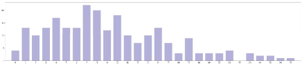
(c) Evolving nodes grouped by the number of active timesteps.

Figure 3. Evolution analysis of the primary school dynamic network.

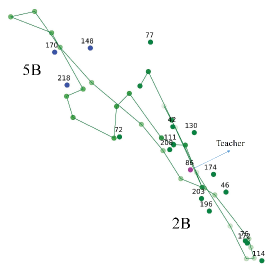
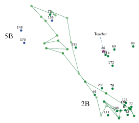
Figure 4. The trajectories of Student 201 (a) and 74 (b).

The primary school data is collected from face-to-face contacts between students and teachers in a school locating in France during two school days in October 2009 (Stehlé et al., 2011). This data contains 232 students from 10 classes, composed of 5 grades with each of the grades divided into two classes. There are 10 assigned teachers for 10 classes. We choose the first day to analyze its evolution patterns due to the similarity between two days. We create a dynamic network with 92 timesteps by a fixed time interval $\Delta t=6$ minutes and a window size $\omega=60$ minutes with an overlap ratio $\gamma=0.9$.

Figure 3(a) shows the projection of students and teachers at 8:45 am (the first graph). We encode each class and teachers with different colors, total eleven colors. Figure 3(b) depicts the number of evolving nodes defined in Section 5.3 from 8:45 am to 17:05 pm. The evolution pattern is in line with the school schedule reported in (Stehlé et al., 2011). Two peak points at 11:40 am and 14:45 pm are two breaks and the low part shows the lunchtime from 12:30 pm to 14:00 pm. Furthermore, few students are extremely active as shown in Figure 3(c).

To analyze the trajectory of active students, we select Student 201 and Student 74 with higher active scores from 8:45 am to 17:05 pm in Figure 4. Student 201 and Student 74 move from Class 2B to Class 5B and then back to Class 2B. Student 201 contacts with the students of Class 5B (e.g., Students 148, 170 and 218) during the lunch break (i.e., from 11:30 am to 13:30 pm), thus we infer they may be friends. We may also conclude that Class 2B and Class 5B share the lunch break, which can be verified from the school schedule. Moreover, we notice that Student 201 contacts with Student 72 after the lunchtime, while Student 74 contacts with Student 72 before the lunchtime. This shows that Student 201 and Student 74 do not have a direct relationship. However, they may be both the friend of Student 72. Based on the triad theory, they will be friends via Student 72.

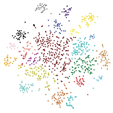
(a) 2D projection of network embeddings colored according to its cluster membership.

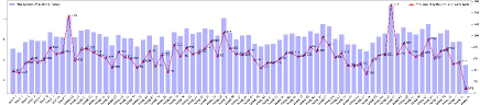
(b) Number of evolving nodes in each timestep.

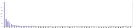
(c) Evolving nodes grouped by the number of active timesteps.

Figure 5. Evolution analysis of the email communication dynamic network.

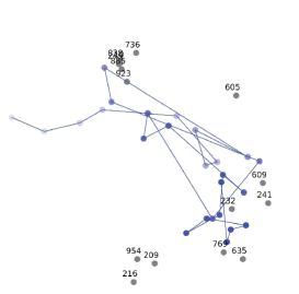
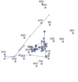
Figure 6. The trajectories of Researcher 90 (a) and 328 (b).

6.2. Email communication dynamic network

The email communication network data is collected from a large European research institution composed of 42 departments (Paranjape et al., 2017). The network data contains 986 nodes and 332,334 temporal edges across 803 days. We create a dynamic network with 74 timesteps by a fixed time interval $\Delta t=7$ days and a window size $\omega=14$ days with an overlap ratio $\gamma=0.5$. The data provider hides all labels of departments for the consideration of personal privacy. To show the proximity of this network, we use DBSCAN (Ester et al., 1996) to cluster nodes based on the L2 distance, and generate 42 clusters. Figure 5(a) shows the clustering result at week 1 via t-SNE. Clusters are colored in different colors. As can be seen from Figure  5(a), this network has a clear structure, and researchers may have more emails with each other in the same department.

The number of evolving nodes at each timestep is provided in Figure 5(b), and the number in each week is relatively stable except few weeks, such as week 10. Most nodes are stable (inactive), as most nodes have zero active weeks (timesteps) in Figure 5(c). We focus on two evolution trajectories of Researcher 90 and Researcher 328 for detailed analysis in Figure 6. Due to the lack of labels, neighbor nodes in the embedded space are colored in gray.

The neighbor nodes of Researcher 90 change over time and we notice Researcher 90 evolves between two groups. In the first few weeks, Researcher 90 has few neighbors, and the reason may be that Researcher 90 joined the institution as a new researcher. After week 51, Researcher 90 leaves his department to another.

Researcher 328 has few neighbors in the first few months. Researcher 90 and Researcher 328 have a similar evolution pattern at the beginning. After that, Researcher 328 moves from the outside of the department to the core position, while the contacts between Researcher 328 and others increases significantly. From the evolution trajectory of Researcher 328, he/she may become a leader or secretary in this department.

7. CONCLUSION

In this paper, we have proposed a novel approach to capturing the changes of dynamic networks with proximity and temporal properties preserved. To evaluate our method, we compare our method with several state-of-the-art methods including static methods and dynamic methods with two tasks, link prediction and evolving node detection. The experiments demonstrate that our method achieves substantial gains and perform effectively in proximity and evolution analysis of dynamic networks. For future work, it is desirable to update nodes which never appear in the network incrementally instead of retraining. Most existing network embedding methods only focus on one noticeable facet of the network, while the network includes diverse facets in the real world. Thus, we would like to design a method to incorporate multiple-facet properties into network embeddings.

References

- (1)
- Bamler and Mandt (2017) Robert Bamler and Stephan Mandt. 2017. Dynamic word embeddings. In Proceedings of the International Conference on Machine Learning. 380–389.
- Cao et al. (2015) Shaosheng Cao, Wei Lu, and Qiongkai Xu. 2015. Grarep: Learning graph representations with global structural information. In Proceedings of the 24th CIKM. ACM, 891–900.
- Cao et al. (2016) Shaosheng Cao, Wei Lu, and Qiongkai Xu. 2016. Deep Neural Networks for Learning Graph Representations. In AAAI. 1145–1152.
- Chen and Sun (2017) Ting Chen and Yizhou Sun. 2017. Task-guided and path-augmented heterogeneous network embedding for author identification. In Proceedings of the Tenth ACM International Conference on Web Search and Data Mining. 295–304.
- Dai et al. (2018) Quanyu Dai, Qiang Li, Jian Tang, and Dan Wang. 2018. Adversarial network embedding. In AAAI. 2167–2174.
- Eger and Mehler (2017) Steffen Eger and Alexander Mehler. 2017. On the linearity of semantic change: Investigating meaning variation via dynamic graph models. In Proceedings of the 54th Annual Meeting of the Association for Computational Linguistics. 52–58.
- Ester et al. (1996) Martin Ester, Hans-Peter Kriegel, Jörg Sander, Xiaowei Xu, et al. 1996. A density-based algorithm for discovering clusters in large spatial databases with noise. In KDD, Vol. 96. 226–231.
- Grover and Leskovec (2016) Aditya Grover and Jure Leskovec. 2016. node2vec: Scalable feature learning for networks. In Proceedings of the 22nd KDD. 855–864.
- Gu et al. (2018) Yupeng Gu, Yizhou Sun, Yanen Li, and Yang Yang. 2018. RaRE: Social Rank Regulated Large-scale Network Embedding. In Proceedings of the 2018 World Wide Web Conference on World Wide Web. 359–368.
- Hamilton et al. (2016) William L Hamilton, Jure Leskovec, and Dan Jurafsky. 2016. Diachronic word embeddings reveal statistical laws of semantic change. In Proceedings of the 54th Annual Meeting of the Association for Computational Linguistics. 1489–1501.
- Hu et al. (2016) Renjun Hu, Charu C Aggarwal, Shuai Ma, and Jinpeng Huai. 2016. An embedding approach to anomaly detection. In Proceedings of the 32nd ICDE. 385–396.
- Kamra et al. (2017) Nitin Kamra, Palash Goyal, Xinran He, and Yan Liu. 2017. DynGEM: Deep Embedding Method for Dynamic Graphs. In IJCAI International Workshop on Representation Learning for Graphs (ReLiG).
- Kulkarni et al. (2015) Vivek Kulkarni, Rami Al-Rfou, Bryan Perozzi, and Steven Skiena. 2015. Statistically significant detection of linguistic change. In Proceedings of the 24th International Conference on World Wide Web. 625–635.
- Kutuzov et al. (2018) Andrey Kutuzov, Lilja Øvrelid, Terrence Szymanski, and Erik Velldal. 2018. Diachronic word embeddings and semantic shifts: a survey. In Proceedings of the 27th International Conference on Computational Linguistics. 1384–1397.
- Ma et al. (2018) Jianxin Ma, Peng Cui, and Wenwu Zhu. 2018. DepthLGP: Learning Embeddings of Out-of-Sample Nodes in Dynamic Networks. In Proceedings of the 32nd AAAI Conference on Artificial Intelligence. 370–377.
- Maaten and Hinton (2008) Laurens van der Maaten and Geoffrey Hinton. 2008. Visualizing data using t-SNE. Journal of machine learning research 9, Nov (2008), 2579–2605.
- Mikolov et al. (2013a) Tomas Mikolov, Kai Chen, Greg Corrado, and Jeffrey Dean. 2013a. Efficient estimation of word representations in vector space. In ICLR Workshop Papers.
- Mikolov et al. (2013b) Tomas Mikolov, Ilya Sutskever, Kai Chen, Greg S Corrado, and Jeff Dean. 2013b. Distributed representations of words and phrases and their compositionality. In Advances in Neural Information Processing Systems. 3111–3119.
- Nguyen et al. (2018) Giang Hoang Nguyen, John Boaz Lee, Ryan A Rossi, Nesreen K Ahmed, Eunyee Koh, and Sungchul Kim. 2018. Continuous-time dynamic network embeddings. In 3rd International Workshop on Learning Representations for Big Networks. 969–976.
- Ni et al. (2018) Jingchao Ni, Shiyu Chang, Xiao Liu, Wei Cheng, Haifeng Chen, Dongkuan Xu, and Xiang Zhang. 2018. Co-Regularized Deep Multi-Network Embedding. In Proceedings of the 2018 World Wide Web Conference on World Wide Web. 469–478.
- Ou et al. (2016) Mingdong Ou, Peng Cui, Jian Pei, Ziwei Zhang, and Wenwu Zhu. 2016. Asymmetric transitivity preserving graph embedding. In Proceedings of the 22nd KDD. 1105–1114.
- Paranjape et al. (2017) Ashwin Paranjape, Austin R Benson, and Jure Leskovec. 2017. Motifs in temporal networks. In Proceedings of the Tenth ACM International Conference on Web Search and Data Mining. 601–610.
- Perozzi et al. (2014) Bryan Perozzi, Rami Al-Rfou, and Steven Skiena. 2014. Deepwalk: Online learning of social representations. In Proceedings of the 20th KDD. 701–710.
- Raftery et al. (2012) Adrian E Raftery, Xiaoyue Niu, Peter D Hoff, and Ka Yee Yeung. 2012. Fast inference for the latent space network model using a case-control approximate likelihood. Journal of Computational and Graphical Statistics 21, 4 (2012), 901–919.
- Ribeiro et al. (2017) Leonardo FR Ribeiro, Pedro HP Saverese, and Daniel R Figueiredo. 2017. struc2vec: Learning node representations from structural identity. In Proceedings of the 23rd KDD. 385–394.
- Robbins and Monro (1985) Herbert Robbins and Sutton Monro. 1985. A stochastic approximation method. In Herbert Robbins Selected Papers. 102–109.
- Rossi and Ahmed (2015) Ryan Rossi and Nesreen Ahmed. 2015. The Network Data Repository with Interactive Graph Analytics and Visualization. In AAAI, Vol. 15. 4292–4293.
- Rudolph and Blei (2018) Maja Rudolph and David Blei. 2018. Dynamic Bernoulli embeddings for language evolution. In Proceedings of the 2018 World Wide Web Conference. 1003–1011.
- Sarkar and Moore (2006) Purnamrita Sarkar and Andrew W Moore. 2006. Dynamic social network analysis using latent space models. In Advances in Neural Information Processing Systems. 1145–1152.
- Stehlé et al. (2011) Juliette Stehlé, Nicolas Voirin, Alain Barrat, Ciro Cattuto, Lorenzo Isella, Jean-François Pinton, Marco Quaggiotto, Wouter Van den Broeck, Corinne Régis, Bruno Lina, et al. 2011. High-resolution measurements of face-to-face contact patterns in a primary school. PloS one 6, 8 (2011), e23176.
- Tang et al. (2015) Jian Tang, Meng Qu, Mingzhe Wang, Ming Zhang, Jun Yan, and Qiaozhu Mei. 2015. Line: Large-scale information network embedding. In Proceedings of the 24th International Conference on World Wide Web. International World Wide Web Conferences Steering Committee, 1067–1077.
- Wang et al. (2016) Daixin Wang, Peng Cui, and Wenwu Zhu. 2016. Structural deep network embedding. In Proceedings of the 22nd KDD. 1225–1234.
- Wang et al. (2017) Xiao Wang, Peng Cui, Jing Wang, Jian Pei, Wenwu Zhu, and Shiqiang Yang. 2017. Community Preserving Network Embedding. In AAAI. 203–209.
- Yao et al. (2018) Zijun Yao, Yifan Sun, Weicong Ding, Nikhil Rao, and Hui Xiong. 2018. Dynamic word embeddings for evolving semantic discovery. In Proceedings of the Eleventh ACM International Conference on Web Search and Data Mining. ACM, 673–681.
- Zhang et al. (2018) Ziwei Zhang, Peng Cui, Jian Pei, Xiao Wang, and Wenwu Zhu. 2018. TIMERS: Error-Bounded SVD Restart on Dynamic Networks. In Proceedings of the 32nd AAAI Conference on Artificial Intelligence. 1–8.
- Zhou et al. (2018) Le-kui Zhou, Yang Yang, Xiang Ren, Fei Wu, and Yueting Zhuang. 2018. Dynamic Network Embedding by Modeling Triadic Closure Process. In AAAI. 571–578.
- Zhu et al. (2016) Linhong Zhu, Dong Guo, Junming Yin, Greg Ver Steeg, and Aram Galstyan. 2016. Scalable temporal latent space inference for link prediction in dynamic social networks. IEEE Transactions on Knowledge and Data Engineering 28, 10 (2016), 2765–2777.