Classical Langevin dynamics derived from quantum mechanics

Abstract.

The classical work by Zwanzig [J. Stat. Phys. 9 (1973) 215-220] derived Langevin dynamics from a Hamiltonian system of a heavy particle coupled to a heat bath. This work extends Zwanzig’s model to a quantum system and formulates a more general coupling between a particle system and a heat bath. The main result proves that ab initio Langevin molecular dynamics, with a certain rank one friction matrix determined by the coupling, approximates for any temperature canonical quantum observables, based on the system coordinates, more accurately than any Hamiltonian system in these coordinates, for large mass ratio between the system and the heat bath nuclei.

1. Langevin molecular dynamics

Langevin dynamics for (unit mass) particle systems with position coordinates $X_{L}:[0,\infty)\to\mathbb{R}^{N}$ and momentum coordinates $P_{L}:[0,\infty)\to\mathbb{R}^{N}$ , defined by

$$\begin{split}{\rm d}X_{L}(t)&=P_{L}(t){\rm d}t\\ {\rm d}P_{L}(t)&=-\nabla\lambda\big{(}X_{L}(t)\big{)}{\rm d}t-\bar{\kappa}P_{L}(t){\rm d}t+(2\bar{\kappa}T)^{1/2}\ {\rm d}W(t)\,,\end{split}$$ (1.1)

is used for instance to simulate molecular dynamics in the canonical ensemble of constant temperature $T$, volume and number of particles, where $W$ denotes the standard Wiener process with $N$ independent components. The purpose of this work is to precisely determine both the potential $\lambda:\mathbb{R}^{N}\to\mathbb{R}$ and the friction matrix $\bar{\kappa}\in\mathbb{R}^{N\times N}$ in this equation, from a quantum mechanical model of a molecular system including weak coupling to a heat bath.

Molecular systems are described by the Schrödinger equation with a potential based on Coulomb interaction of all nuclei and electrons in the system. This quantum mechanical model is complete in the sense that no unknown parameters enter - the observables in the canonical ensemble are determined from the Hamiltonian and the temperature. The classical limit of the quantum formulation, yields an accurate approximation of the observables based on the nuclei only, for large nuclei–electron mass ratio $M$. Ab initio molecular dynamics based on the electron ground state eigenvalue can be used when the temperature is low compared to the first electron eigenvalue gap. A certain weighted average of different ab initio dynamics, corresponding to each electron eigenvalue, approximates quantum observables for any temperature, see [10], also in the case of observables including time correlation and many particles. The elimination of the electrons provides a substantial computational reduction, making it possible to simulate large molecular systems, cf. [18].

In molecular dynamics simulations one often wants to determine properties of a large macroscopic system with many particles, say $N\sim 10^{23}$. Such large particle systems cannot yet be simulated on a computer and one may then ask for a setting where a smaller system has similar properties as the large. Therefore, we seek an equilibrium density that has the property that the marginal distribution for a subsystem has the same density as the whole system. In [10] it is motivated how this assumption leads to the Gibbs measure, i.e. the canonical ensemble; this is also the motivation to use the canonical ensemble for the composite system in this work, although some studies on heat bath models use the microcanonical ensemble for the composite whole system.

Langevin dynamics is often introduced to sample initial configurations from the Gibbs distribution and to avoid to simulate the dynamics of all heat bath particles. The friction/damping parameter in the Langevin equation is then typically set small enough to not perturb the dynamics too much and large enough to avoid long sampling times.

The purpose of this work is to show that Langevin molecular dynamics, for the non heat bath nuclei, with a certain friction/damping parameter determined from the Hamiltonian, approximates the quantum system, in the canonical ensemble for any temperature, more accurately than any Hamiltonian dynamics (for the non heat bath particles) in the case the system is weakly coupled to a heat bath of many fast particles.

Our heat bath model is based on the assumption of weak coupling - in the sense that the perturbation in the system from the heat bath is small and vice versa - which we show leads to Zwanzig’s model for nonlinear generalized Langevin equations in [27], with a harmonic oscillator heat bath. Zwanzig also derives a pure Langevin equation: he assumes first a continuous Debye distribution of the eigenvalues of the heat bath potential energy quadratic form; in the next step he lets the coupling to the heat bath have a special form, so that the integral kernel for the friction term in the generalized Langevin equation becomes a Dirac-delta measure. Our derivation uses a heat bath based on nearest neighbour interaction on an infinite cubic lattice, so that the continuum distribution of eigenvalues is rigorously obtained by considering a difference operator with an infinite number of nodes. Our convergence towards a pure Langevin equation is not based on a Dirac-delta measure for the integral kernel but obtained from the time scale separation of the fast heat bath particles and the slower system particles, which allows a general coupling and a bounded covariance matrix for the fluctuations. The fast heat bath dynamics is provided either from light heat bath particles or a stiff heat bath potential. By a stiff heat bath we mean that the smallest eigenvalue of the Hessian of the heat bath potential energy is of the order $\chi^{-1}$, where $\chi\ll 1$. We show that the friction/damping coefficient in the pure Langevin equation is determined by the derivative of the forces on the heat bath particles with respect to the system particle positions. We also prove that the observables of the system coordinates in the system-heat bath quantum model can be approximated using this Langevin dynamics with accuracy $\mathcal{O}(m\log m^{-1}+(mM)^{-1})$, where $M\gg 1$ is the system nuclei–electron mass ratio and $m\ll 1$ is the heat bath nuclei – system nuclei mass ratio; the approximation by a Hamiltonian system yields the corresponding larger error estimate $\mathcal{O}(m^{1/2}+(mM)^{-1})$, in the case of light heat bath particles. In this sense, our Langevin equation is a better approximation. The case with a stiff heat bath system has the analogous error estimate $\mathcal{O}(\chi^{2\delta}\log\chi^{-1}+M^{-1})$ with the correct friction/damping parameter, while a Hamiltonian system gives the larger error $\mathcal{O}(\chi^{2\delta-1/2}+M^{-1})$, where $\chi^{\delta}\ll\chi^{1/4}$ measures the coupling between the heat bath and the system. Our main assumptions are:

• the coupling between the system and the heat bath is weak and localized,

• either the heat bath particles are much lighter than the system particles or the heat bath is stiff,

• the harmonic oscillator heat bath is constructed from nearest neighbour interaction on an infinite cubic lattice in dimension three,

• the heat bath particles are initially randomly Gibbs distributed (conditioned by the system particle coordinates), and

• the system potential energy and the observables are sufficiently regular.

The system and the heat bath is modelled by a Hamiltonian where the system potential energy is perturbed by $\bar{V}(x,X)$ with system particle positions $X\in\mathbb{R}^{N}$ and heat bath particle positions $x\in\mathbb{R}^{n}$. Our assumption of weak coupling is formulated as the requirement that the potential $\bar{V}$ satisfies

$$\min_{x\in\mathbb{R}^{n}}\bar{V}(x,X)=\bar{V}\big{(}a(X),X\big{)}=0\,.$$

Theorem 3.7 proves that the obtained minimizer $a(X)\in\mathbb{R}^{n}$ determines the friction matrix $\bar{\kappa}$ in (1.1) by the rank one $N\times N$ matrix

$$\bar{\kappa}_{\ell\ell^{\prime}}=\bar{c}m^{1/2}\langle\bar{V}^{\prime\prime}(a,X)\partial_{X_{\ell}}a,\bar{V}^{\prime\prime}(a,X)\partial_{X_{\ell^{\prime}}}a\rangle\,,$$

where $\bar{V}$ and $a$ have limits as $n\to\infty$; here $\bar{V}^{\prime\prime}$ denotes the Hessian of $\bar{V}$ with respect to $x$, the brackets $\langle\cdot,\cdot\rangle$ denote the scalar product in $\mathbb{R}^{n}$ and $\bar{c}$ is a constant (related to the density of states).

In a setting when the temperature is small compared to the difference of the two smallest eigenvalues of the Hamiltonian symbol, with given nuclei coordinates, it is well known that ab initio molecular dynamics is based on the ground state electron eigenvalue as the potential $\lambda$ in (1.1), cf. [18]. When the temperature is larger, excited electron states influence the nuclei dynamics. The work [10] derives a molecular dynamics approximation of quantum observables, including time correlations, as a certain weighted average of ab initio observables in the excited states, and these ideas are put into the context of this work in Section 5.

The analysis of particles in a heat bath has a long history, starting with the work by Einstein and Smoluchowski. The Langevin equation was introduced in [14] to study Brownian motion mathematically, before the Wiener process was available. Early results on the elimination of the heat bath degrees of freedom to obtain a Langevin equation are [7, 6] and [27],[26, Section 9.3]. The work [7, 6] include in addition a derivation of a quantum Langevin equation, which is based on an operator version of the classical Langevin equation. Our study of the classical Langevin equation from quantum mechanics is not related to this quantum Langevin equation. We start with an ab initio quantum model of the system coupled to a heat bath in the canonical ensemble and use its classical limit to eliminate the electron degrees of freedom. Then the classical system coupled to the heat bath is analyzed by separation of time scales. The separation of time scales of light bath particles and heavier system particles was first used in [15], see also [20, 23] to determine a Fokker-Planck equation for the system particle, from the Liouville equation of the coupled system using a formal expansion in the small mass ratio. Section 8 in [22] presents a proof, and several references to related work, where the Langevin equation is derived from the generalized Langevin equation, using exponential decay of the kernel in the memory term of the generalized Langevin equation.

Our contribution employs the separation of time scales approach previously used in [15, 20, 23], but a novelty is that we here present mathematical proofs for the weak convergence rate of Langevin dynamics towards quantum mechanics. Our work also differs from [22, Section 8], wherein the kernel of the generalized Langevin equation is assumed to be such that by adding a finite dimensional variable the system becomes Markovian and the kernel tends to a point mass. For instance, our kernel vanishes as $m\to 0^{+}$ and we use the density of heat bath states to determine the kernel. Using the precise information from the density of states in the case of heat bath nearest neighbor interaction in a cubic lattice we obtain a positive definite friction matrix $\bar{\kappa}$, while if the nearest neighbor interaction would be related to a lattice in dimension four the friction matrix would vanish, see Remark 3.4.

The main new ideas in our work are the first principles formulation from quantum mechanics, the weak coupling condition as a minimization, the precise use of the density of heat bath states, that the error estimate uses stability of the Kolmogorov backward equation for the Langevin equation evaluated along the dynamics of the coupled system, and formulation of numerical schemes and numerical results related to Langevin dynamics approximation of particles systems.

Section 2 formulates a classical model for the system and the heat bath, including the weak coupling, and derives the corresponding generalized Langevin equation, based on a memory term with a specific integral kernel, in a classical molecular dynamics setting. The generalized Langevin equation is analyzed in Section 3, with subsections related to the dissipation, fluctuations and approximation by pure Langevin dynamics in the case of light heat bath particles. The main result of Section 3 is Theorem 3.7, where a certain Langevin dynamics is shown to approximate a classical system weakly coupled to a heat bath. Section 4 extends the analysis to the case of stiff heat baths and derives a corresponding approximation result in Theorem 4.1. Section 5 relates the classical model to a quantum formulation and provides background and error estimates on quantum observables in the canonical ensemble approximated by classical molecular dynamics. The main result of the work is Theorem 5.2, which proves that for any temperature canonical quantum observables based on the system coordinates can be accurately approximates by the Langevin dynamics obtained in Theorems 3.7 and 4.1. Section 6 includes numerical results of the system particle density and autocorrelation of the coupled system and heat bath approximated by the particle density and autocorrelation for the Langevin dynamics.

2. The model of the system and the heat bath

We consider in this section a classical model of a molecular system, with position coordinates $X\in\mathbb{R}^{N}$ and momentum coordinates $P\in\mathbb{R}^{N}$, coupled to a heat bath, with position and momentum coordinates $x\in\mathbb{R}^{n}$ and $p\in\mathbb{R}^{n}$, respectively, represented by the Hamiltonian

$$\frac{|P|^{2}}{2}+\frac{|p|^{2}}{2m}+\lambda(X)+\bar{V}(x,X)\,,$$

where $\lambda:\mathbb{R}^{N}\to\mathbb{R}$ is the potential energy for the system and $\bar{V}:\mathbb{R}^{n}\times\mathbb{R}^{N}\to\mathbb{R}$ is the potential energy for the heat bath including the coupling to the system. The parameter $m$ is the mass ratio between heat bath nuclei and system nuclei. We have set the time scale so that the system nuclei mass is one. In Section 5 we show that this model is the classical limit of a quantum model and study the accuracy of the classical approximation, also in the case with system nuclei that have different masses.

We study small perturbations of the equilibrium bath state $x=a(X)\in\mathbb{R}^{n}$ where

$$\min_{x\in\mathbb{R}^{n}}\bar{V}(x,X)=\bar{V}\big{(}a(X),X\big{)}\,.$$

Taylor expansion around the equilibrium yields

$$\bar{V}(x,X)=\bar{V}\big{(}a(X),X\big{)}+\frac{1}{2}\big{\langle}x-a(X),\bar{V}^{\prime\prime}_{xx}\big{(}a(X)+\xi(x-a(X)),X\big{)}\big{(}x-a(X)\big{)}\big{\rangle}$$

for some $\xi\in[0,1]$, where $\bar{V}_{xx}$ is the Hessian matrix in $\mathbb{R}^{n\times n}$, with respect to the $x$ coordinate, and the notation $\langle\cdot,\cdot\rangle$ is the standard scalar product in $\mathbb{C}^{n}$. We assume that the coupling between the system and the heat bath is weak, which means that the perturbation in the system from the heat bath must be small. As the perturbation $|x-a(X)|\to 0$ we therefore require that

$$\bar{V}(a(X),X)=0\,.$$ (2.1)

Weak coupling also means that the perturbation in the heat bath from the system is small, so that the influence on the Hessian $\bar{V}^{\prime\prime}_{xx}$ from $X$ is negligible, and we assume therefore that

$$\bar{V}_{xx}^{\prime\prime}\big{(}a(X)+\xi(x-a),X\big{)}=C$$ (2.2)

where $C$ is constant, symmetric and positive definite. Hence the vibration frequencies for $x$ are assumed to be constant for all $x$ and $X$. We use the notation $C=\bar{V}^{\prime\prime}$ below.

The assumptions (2.1) and (2.2) of weak coupling lead to the Hamiltonian $H:\mathbb{R}^{N}\times\mathbb{R}^{N}\times\mathbb{R}^{n}\times\mathbb{R}^{n}\to\mathbb{R}$

$$H(X,P,x,p)=\frac{|P|^{2}}{2}+\frac{|p|^{2}}{2m}+\lambda(X)+\frac{1}{2}\langle\bar{V}^{\prime\prime}\big{(}x-a(X)\big{)},\,x-a(X)\rangle\,.$$ (2.3)

This model (2.3) is of the same form as the model of interaction with a heat bath introduced and analysed by Zwanzig in the seminal work [27], although here the motivation with weak coupling and several system particles is different.

The Hamiltonian (2.3) yields the dynamics

$$\begin{split}\dot{X}_{t}&=P_{t}\\ \dot{P}_{t}&=-\nabla\lambda(X_{t})+\langle\bar{V}^{\prime\prime}\big{(}x_{t}-a(X_{t})\big{)},\nabla a(X_{t})\rangle\\ \dot{x}_{t}&=p_{t}/m\\ \dot{p}_{t}&=-\bar{V}^{\prime\prime}\big{(}x_{t}-a(X_{t})\big{)}\,\end{split}$$

and the change of variables $(m\bar{V}^{\prime\prime})^{1/2}r_{t}:=p_{t}$ implies

$$\begin{split}\dot{x}_{t}&=m^{-1/2}\bar{V}^{\prime\prime 1/2}r_{t}\\ \dot{r}_{t}&=-m^{-1/2}\bar{V}^{\prime\prime 1/2}\big{(}x_{t}-a(X_{t})\big{)}\,.\end{split}$$

Define $\varphi_{t}:=x_{t}-a(X_{t})+{\rm i}r_{t}$ to obtain

$$\begin{split}\dot{X}_{t}&=P_{t}\\ \dot{P}_{t}&=-\nabla\lambda(X_{t})+{\rm Re}\langle\bar{V}^{\prime\prime}\varphi_{t},\nabla a(X_{t})\rangle\\ {\rm i}\dot{\varphi}_{t}&=m^{-1/2}\bar{V}^{\prime\prime 1/2}\varphi_{t}-{\rm i}\dot{X}_{t}\cdot\nabla a(X_{t})\,,\end{split}$$ (2.4)

where the third equation uses the notation $v\cdot w$ for the standard scalar product in $\mathbb{R}^{N}$.

Assume that $x_{0}$ and $p_{0}$ are Gaussian with the distributions provided by the marginals of the Gibbs density

$$\frac{e^{-H(X,P,x,p)/T}}{\int_{\mathbb{R}^{2N+2n}}e^{-H(X,P,x,p)/T}{\rm d}X{\rm d}P{\rm d}x{\rm d}p}\,,$$

that is, the momentum $p$ is multivariate normal distributed with mean zero and covariance matrix $mT\,{\rm I}$ and independent of $x$, which is multivariate normal distributed with mean $a(X)$ and covariance matrix $T(\bar{V}^{\prime\prime})^{-1}$. Consequently the initial data can be written

$$\varphi_{0}=\sum_{k=1}^{n}\gamma_{k}\nu_{k}^{\prime}$$ (2.5)

using the orthogonal eigenvectors $\nu_{m}^{\prime}$, normalized as $\langle\nu^{\prime}_{k},\nu^{\prime}_{k}\rangle=1$, and eigenvalues $\mu_{m}$ of $\bar{V}^{\prime\prime}$

$$\begin{split}\bar{V}^{\prime\prime}\nu_{m}^{\prime}&=\mu_{m}\nu_{m}^{\prime}\,,\quad\nu_{m}^{\prime}\in\mathbb{R}^{n}\mbox{ and }\mu_{m}\in\mathbb{R}_{+}\end{split}$$ (2.6)

and the definition

$$\gamma_{m}:=\gamma_{m}^{r}+{\rm i}\gamma_{m}^{i}$$ (2.7)

with $\gamma_{m}^{r}$ and $\gamma_{m}^{i},\ m=1,\ldots,n$, independent and normal distributed real scalar random numbers with mean zero and variance $T/\mu_{m}$.

Duhamel’s principle shows that

$$\varphi_{t}=e^{-{\rm i}\bar{V}^{\prime\prime 1/2}m^{-1/2}t}\varphi_{0}-\int_{0}^{t}e^{-{\rm i}\bar{V}^{\prime\prime 1/2}m^{-1/2}(t-s)}\dot{a}(X_{s}){\rm d}s$$

which implies a form of Zwanzig’s generalized Langevin equation

$$\begin{split}\ddot{X}_{t}&=-\nabla\lambda(X_{t})-\int_{0}^{t}\langle\bar{V}^{\prime\prime}\cos\big{(}\frac{(t-s)\bar{V}^{\prime\prime 1/2}}{m^{1/2}}\big{)}\dot{a}(X_{s}),\nabla a(X_{t})\rangle{\rm d}s\\ &\quad+{\rm Re}\langle\bar{V}^{\prime\prime}e^{-{\rm i}\bar{V}^{\prime\prime 1/2}m^{-1/2}t}\varphi_{0},\nabla a(X_{t})\rangle\,,\end{split}$$ (2.8)

with non Markovian friction term given by the integral and a noise term including the stochastic initial data $\varphi_{0}$. We study two different cases:

• either the mass ratio $m\ll 1$ is small, or

• the smallest eigenvalue of $\bar{V}^{\prime\prime}$ is large of the order $\chi^{-1}$ while the coupling derivative $\|\nabla a\|$ is small of size $\chi^{\delta}$ with $\delta>1/4$.

In these cases, both the friction and the noise terms are based on highly oscillatory functions, which will make these contributions small, as explained in the next section. To simplify the analysis, we assume also that

$$\nabla a(\cdot)$$ is constant. (2.9)

3. Analysis of the generalized Langevin equation for $m\ll 1$

In this section we first study the dissipation term $\int_{0}^{t}\langle\bar{V}^{\prime\prime}\cos\big{(}\frac{(t-s)\bar{V}^{\prime\prime 1/2}}{m^{1/2}}\big{)}\dot{a}(X_{s}),\nabla a\rangle{\rm d}s$ and the fluctuation term ${\rm Re}\langle\bar{V}^{\prime\prime}e^{-{\rm i}\bar{V}^{\prime\prime 1/2}m^{1/2}t}\varphi_{0},\nabla a\rangle$ in (2.8), as the number of bath particles tend to infinity and the mass ratio, $m$, between light heat bath nuclei and heavier system nuclei is small. Then in Section 3.3 we prove an priori estimate of $\sup_{s<t}\mathbb{E}[|X_{s}|^{2}+|\dot{X}_{s}|^{2}+|\ddot{X}_{s}|^{2}]$. Section 3.4 uses the limit terms to construct a Langevin equation, namely the Itô stochastic differential equation

$$\begin{split}{\rm d}X_{L}(t)&=P_{L}(t){\rm d}t\\ {\rm d}P_{L}(t)&=-\nabla\lambda\big{(}X_{L}(t)\big{)}{\rm d}t-m^{1/2}\kappa P_{L}(t){\rm d}t+(2m^{1/2}\kappa T)^{1/2}\ {\rm d}W(t)\,,\end{split}$$ (3.1)

with a certain symmetric friction matrix $\kappa\in\mathbb{R}^{N\times N}$ and a Wiener process $W:[0,\infty)\times\Omega\to\mathbb{R}^{N}$, with $N$ independent components; here $\Omega$ is the set of outcomes for the process $(X,P):[0,\infty)\times\Omega\to\mathbb{R}^{2N}$. Finally, we use the solution of the Kolmogorov backward equation for the Langevin dynamics along a solution path $(X_{t},P_{t})$ of (2.8) to derive an error estimate of the approximation, namely $\mathbb{E}[g(X_{t},P_{t})]-\mathbb{E}[g(X_{L}(t),P_{L}(t)]=\mathcal{O}(m\log m^{-1})$, for any given smooth bounded observable $g:\mathbb{R}^{2N}\to\mathbb{R}$ and equal initial data $(X(0),P(0))=(X_{L}(0),P_{L}(0))$.

3.1. The dissipation term and a precise heat bath

The change of variables

$$\frac{t-s}{m^{1/2}}=\tau$$

yields

$$\begin{split}&\int_{0}^{t}\langle\bar{V}^{\prime\prime}\cos\big{(}\frac{(t-s)V^{\prime\prime 1/2}}{m^{1/2}}\big{)}\dot{a}(X_{s}),\partial_{X^{\ell}}a\rangle{\rm d}s\\ &=m^{1/2}\int_{0}^{t/\sqrt{m}}\langle\bar{V}^{\prime\prime}\cos(\tau\bar{V}^{\prime\prime 1/2})\dot{a}(X_{t-m^{1/2}\tau}),\partial_{X^{\ell}}a\rangle{\rm d}\tau\\ &=\sum_{\ell^{\prime}}m^{1/2}\int_{0}^{t/\sqrt{m}}\langle\bar{V}^{\prime\prime}\cos(\tau\bar{V}^{\prime\prime 1/2})\partial_{X^{\ell^{\prime}}}a,\partial_{X^{\ell}}a\rangle\dot{X}^{\ell^{\prime}}_{t-\sqrt{m}\tau}{\rm d}\tau\,.\end{split}$$

We require this dissipation term to be small, so that the coupling to the heat bath yields a small perturbation of the dynamics for $X$ and $P$. If $\bar{V}^{\prime\prime}$ and $\nabla a$ are of order one, the mass $m$ needs to be small, or if $\nabla a$ is small we can have $\bar{V}^{\prime\prime}$ large. The case with small $m$ is studied in this section and the case with large $\bar{V}^{\prime\prime}$ is in Section 4.

A small mass also requires the integrand to decay as $\tau\to\infty$. We will use Fourier analysis to study the decay of the kernel

$$K_{n}^{\ell\ell^{\prime}}:=\langle\bar{V}^{\prime\prime}\cos(\tau\bar{V}^{\prime\prime 1/2})\partial_{X^{\ell^{\prime}}}a,\partial_{X^{\ell}}a\rangle\,,$$

by writing $\lim_{n\to\infty}K_{n}$ as an integral, which is the next step in the analysis.

The kernel $K_{n}$ is based on the equilibrium heat bath position derivative $\partial_{X^{\ell}}a$ and this derivative is determined by the derivative of the force on bath particle $x_{j}$, with respect to $X^{\ell}$, by (2.3) as

$$F^{\prime}_{\ell,j}:=-\partial_{X^{\ell}}\partial_{x_{j}}\bar{V}(x,X)=(\bar{V}^{\prime\prime}\partial_{X^{\ell}}a)_{j}\,,$$

which, for fixed $\ell$ and $j$, by assumptions (2.2) and (2.9) is independent of $x$ and $X$. We assume that $\bar{V}$ is constructed so that this force derivative is localized in the sense

$$\begin{split}&\sum_{j}|F^{\prime}_{\ell,j}|(1+|j-\hat{\ell}|^{2})=\mathcal{O}(1)\,,\quad\mbox{ as $n\to\infty$, for $\hat{\ell}:={\rm argmin}_{j}|X_{\ell}-x_{j}|$}\\ &\mbox{ $\lim_{n\to\infty}F^{\prime}_{\ell,j}$ exists.}\end{split}$$ (3.2)

Let $\nu_{k}(j):=\nu_{k}^{\prime}(j)/\max_{j}|\nu_{k}^{\prime}(j)|$ be the set of orthogonal eigenvectors of $\bar{V}^{\prime\prime}$ that are normalized to one in the maximum norm.The eigenvalue representation of $\bar{V}^{\prime\prime}$ in (2.6) and the definition

$$\omega_{k}^{2}={\mu_{k}}$$

yields

$$\begin{split}\beta_{\ell,k}&:=\sum_{j}F^{\prime}_{\ell,j}\nu_{k}^{*}(j)=\langle\nu_{k},F^{\prime}_{\ell\cdot}\rangle\,,\\ F^{\prime}_{\ell,j}&=(\bar{V}^{\prime\prime}\partial_{X^{\ell}}a)_{j}=\sum_{k}\frac{\beta_{\ell,k}}{\|\nu_{k}\|^{2}_{2}}\nu_{k}(j)\,,\\ \partial_{X^{\ell}}a_{j}&=\sum_{k}\frac{\beta_{\ell,k}}{\omega_{k}^{2}\,\|\nu_{k}\|^{2}_{2}}\nu_{k}(j)\,,\\ \end{split}$$ (3.3)

where $\|\nu_{k}\|_{2}:=(\sum_{j}|\nu_{k}(j)|^{2})^{1/2}$. Consequently we obtain

$$\begin{split}K_{n}^{\ell\ell^{\prime}}(\tau)&=\langle\bar{V}^{\prime\prime}\cos(\tau\bar{V}^{\prime\prime 1/2})\partial_{X^{\ell}}a,\partial_{X^{\ell^{\prime}}}a\rangle\\ &=\sum_{k}\cos(\tau\omega_{k})\frac{\beta_{\ell,k}^{*}\beta_{\ell^{\prime},k}}{\omega_{k}^{2}\,\|\nu_{k}\|_{2}^{2}}\,.\\ \end{split}$$ (3.4)

If $n$ is finite and we make a tiny perturbation of $\bar{V}^{\prime\prime}$ so that all $\omega_{k}$ become rational, the function $K_{n}$ will be periodic in $\tau$ and consequently it will not decay for large $\tau$. To obtain a decaying kernel we will therefore consider a heat bath with infinite number of particles, $n=\infty$. The next step is consequently to study the limit of $K_{n}$, as $n\to\infty$, which requires a more precise formulation of the heat bath.

3.1.1. A precise heat bath

We use the periodic lattice

$$E_{\bar{n}}:=\{-\bar{n}/2,-\bar{n}/2+1,\ldots,\bar{n}/2-1\}^{3}\subset\mathbb{R}^{3}$$

in dimension three to form the equilibrium positions for the heat bath. The position deviation from the equilibrium, namely $\bar{x}_{j}:=x_{j}-a_{j}(X)\in\mathbb{R}$ for each particle $j\in E_{\bar{n}}$, then determines the potential by nearest neighbour interaction in the lattice

$$\begin{split}\langle\bar{V}^{\prime\prime}\bar{x},\bar{x}\rangle&=c^{2}\sum_{i=1}^{3}\sum_{j\in E_{\bar{n}}}|\bar{x}_{j+e_{i}}-\bar{x}_{j}|^{2}+\eta_{n}^{2}\sum_{i=1}^{3}\sum_{j\in E_{\bar{n}}}|\bar{x}_{j+e_{i}}|^{2}\\ &=c^{2}\sum_{i=1}^{3}\sum_{j\in E_{\bar{n}}}(-\bar{x}_{j+e_{i}}+2\bar{x}_{j}-\bar{x}_{j-e_{i}})\bar{x}_{j}+\eta_{n}^{2}\sum_{i=1}^{3}\sum_{j\in E_{\bar{n}}}|\bar{x}_{j+e_{i}}|^{2}\\ \end{split}$$ (3.5)

with periodic boundary conditions $\bar{x}_{j+\bar{n}e_{i}}=\bar{x}_{j}$, where $j=(j_{1},j_{2},j_{3}),\ e_{1}=(1,0,0),e_{2}=(0,1,0),e_{3}=(0,0,1)$, $\bar{n}^{3}=n$ and $c$ is a positive constant independent of $n$. The small positive constant $\eta_{n}$ is introduced to make the potential strictly convex for finite $n$, while it vanishes asymptotically and satisfies

$$n^{1/2}\eta_{n}\to\infty\mbox{ and }\eta_{n}\to 0^{+}\ \mbox{ as }n\to\infty\,.$$ (3.6)

We will see in (3.19) that the zero limit in (3.6) is needed in our model to obtain non zero friction matrices $\kappa$. The lower bound in (3.6) implies by (3.3) that $\|\partial_{X^{\ell}}a\|_{\ell^{\infty}}$ remains bounded, provided $\|\beta_{\ell,\cdot}\|_{\ell^{1}}$ is bounded. We note that $\bar{V}^{\prime\prime}$ consists of the standard finite difference matrix with mesh size one related to the Laplacian in $\mathbb{R}^{3}$ and a small positive definite perturbation $\eta_{n}^{2}\,{\rm I}$, where ${\rm I}$ is the corresponding identity matrix. The minimum of the potential is obtained for the position deviations $\bar{x}_{j}=0,\ j\in E_{\bar{n}}$, which we may view as the $n$ heat bath particles located on the $n$ different lattice points in $E_{\bar{n}}$. This heat bath model can be extended to positions $\bar{x}_{j}\in\mathbb{R}^{3}$, see Remark 3.1.

In each coordinate direction the discrete Laplacian is a circulant matrix so that the eigenvectors and eigenvalues can be written

$$\begin{split}\nu_{k}(j)&=e^{2\pi{\rm i}j\cdot k/\bar{n}}\quad,\,j_{i}=-\bar{n}/2,\ldots,\bar{n}/2-1,\mbox{ and }\ k_{i}=-\bar{n}/2,\ldots,\bar{n}/2-1\,,\\ \omega_{k}^{2}&=c^{2}\sum_{i=1}^{3}2\big{(}1-\cos(\frac{2\pi k_{i}}{\bar{n}})\big{)}+\eta_{n}^{2}\,,\\ \end{split}$$ (3.7)

and $\|\nu_{k}\|_{2}^{2}=\sum_{i=1}^{3}\sum_{j_{i}=-\bar{n}/2}^{\bar{n}/2-1}|\nu_{k}(j)|^{2}=\bar{n}^{3}$. Let $\mathbf{r}:=(\frac{k_{1}}{\bar{n}},\frac{k_{2}}{\bar{n}},\frac{k_{3}}{\bar{n}})$ and $r:=\sqrt{k_{1}^{2}+k_{2}^{2}+k_{3}^{2}}/\bar{n}$. We have for $k=\bar{n}\mathbf{r}$ by (3.6)

$$\begin{split}\nu_{k}(j)&=e^{2\pi{\rm i}j\cdot\mathbf{r}}=:\nu(\mathbf{r},j)\,,\\ \lim_{n\to\infty}\omega_{k}^{2}&=c^{2}\sum_{i=1}^{3}2\big{(}1-\cos(2\pi r_{i})\big{)}=:\big{(}\omega(\mathbf{r})\big{)}^{2}\,,\\ \end{split}$$

and we assume that the derivative of the force has a limit

$$\lim_{n\to\infty}F^{\prime}_{\ell,j}=\bar{F}_{\ell,j}\,,$$ (3.8)

which implies

$$\begin{split}\lim_{{\tiny\begin{array}[]{c}n\to\infty\\ \frac{k}{\bar{n}}=\mathbf{r}\end{array}}}\beta_{\ell,k}&=\sum_{j\in E_{\infty}}\bar{F}_{\ell,j}\nu^{*}(\mathbf{r},j)=:\beta_{\ell}(\mathbf{r})\,,\\ \beta_{\ell}(0)&=\sum_{j\in E_{\infty}}\bar{F}_{\ell,j}\,,\end{split}$$ (3.9)

that is, the function $\beta_{\ell}:[-1/2,1/2]^{3}\to\mathbb{R}$ has the Fourier coefficients $\bar{F}_{\ell,j}$. The value $\beta_{\ell}(0)$ will be used in (3.19) to determine the friction matrix $\kappa$.

Remark 3.1.

The heat bath model (3.5) can be extended to have $\bar{x}_{j}=x_{j}-a_{j}(X)\in\mathbb{R}^{3}$, with $\bar{x}_{j}=({\bar{x}_{j}^{1}},{\bar{x}_{j}^{2}},{\bar{x}_{j}^{3}})$. In the case

$$\langle\bar{V}^{\prime\prime}\bar{x},\bar{x}\rangle=\sum_{k=1}^{3}\sum_{i=1}^{3}\sum_{j\in E_{\bar{n}}}c_{k}^{2}(-{\bar{x}_{j+e_{i}}^{k}}+2{\bar{x}_{j}^{k}}-{\bar{x}_{j-e_{i}}^{k}}){\bar{x}_{j}^{k}}+\eta_{n}^{2}\sum_{i=1}^{3}\sum_{j\in E_{\bar{n}}}|\bar{x}_{j+e_{i}}|^{2}$$

we still have the same eigenvalues if $c_{k}^{2}=c^{2}$, so the model does not change in principle. If on the other hand the constants $c_{k}$ are different for the different components of $\bar{x}_{j}$ the spectrum may change and we obtain a different heat bath model.

3.1.2. The limit friction matrix

We can take the limit as $\bar{n}\to\infty$ in (3.4), while $\mathbf{r}=k/\bar{n}$ is constant, to obtain an integral

$$\begin{split}\lim_{n\to\infty}K_{n}^{\ell\ell^{\prime}}(\tau)&=\lim_{n\to\infty}\sum_{k}\cos(\tau\omega_{k})\frac{\beta_{\ell,k}^{*}\beta_{\ell^{\prime},k}}{\omega_{k}^{2}\|\nu_{k}\|_{2}^{2}}\\ &=\int_{[-\frac{1}{2},\frac{1}{2}]^{3}}\cos\big{(}\tau\omega(\mathbf{r})\big{)}\frac{\beta_{\ell}^{*}(\mathbf{r})\beta_{\ell^{\prime}}(\mathbf{r})}{\big{(}\omega(\mathbf{r})\big{)}^{2}}{\rm d}r_{1}{\rm d}r_{2}{\rm d}r_{3}\\ &=:K_{\infty}^{\ell\ell^{\prime}}(\tau)\,.\end{split}$$ (3.10)

The change of variables $\omega_{i}=2^{1/2}c\sqrt{1-\cos(2\pi r_{i})}\,{\rm sgn}(r_{i})$ yields, with the spherical coordinate $\boldsymbol{\omega}=(\cos\alpha\cos\theta,\sin\alpha\cos\theta,\sin\theta)\omega$,

$$\begin{split}&\lim_{n\to\infty}\sum_{k}\cos(\tau\omega_{k})\frac{\beta_{\ell,k}^{*}\beta_{\ell^{\prime},k}}{\omega_{k}^{2}\|\nu_{k}\|_{2}^{2}}\\ &=\int_{{\boldsymbol{\omega}}([-\frac{1}{2},\frac{1}{2}]^{3})}\cos(\tau\omega)\beta_{\ell}^{*}(\mathbf{r}(\boldsymbol{\omega}))\beta_{\ell^{\prime}}(\mathbf{r}(\boldsymbol{\omega}))\prod_{i=1}^{3}\Big{(}\frac{\sqrt{1-\cos\big{(}2\pi r_{i}(\omega_{i})\big{)}}}{2^{1/2}\pi c\sin\big{(}2\pi r_{i}(\omega_{i})\big{)}}\Big{)}\frac{{\rm d}\boldsymbol{\omega}}{|\omega|^{2}}\\ &=\int_{{\boldsymbol{\omega}}([-\frac{1}{2},\frac{1}{2}]^{3})}\cos(\tau\omega)f(\boldsymbol{\omega},\ell,\ell^{\prime})\frac{{\rm d}\boldsymbol{\omega}}{|\omega|^{2}}\\ &=\int_{0}^{\pi}\int_{0}^{2\pi}\int_{0}^{\infty}\cos(\tau\omega)f(\boldsymbol{\omega},\ell,\ell^{\prime})\sin\theta{\rm d}\omega{\rm d}\alpha{\rm d}\theta\\ \end{split}$$

where

$$f(\boldsymbol{\omega},\ell,\ell^{\prime}):=\begin{cases}\beta_{\ell^{\prime}}(\boldsymbol{\omega})\beta_{\ell}^{*}(\boldsymbol{\omega})\prod_{i=1}^{3}\pi^{-1}\big{(}4c^{2}-{\omega_{i}^{2}}\big{)}^{-1/2}\,,&-2c<\omega_{i}<2c\,,\\ 0\,,&\mbox{ otherwise}\,.\\ \end{cases}$$ (3.11)

with $\beta(\boldsymbol{\omega}):=\beta(r(\boldsymbol{\omega}))$. The term $(4c^{2}-\omega_{i}^{2})^{-1/2}$ is unbounded (but integrable) at the boundary where $\omega_{i}=\pm 2c$. For the purpose of simplifying later proofs we will assume that $\beta_{\ell}(\boldsymbol{\omega})$ is two times differentiable and that it vanishes at the boundary of ${\boldsymbol{\omega}}([-\frac{1}{2},\frac{1}{2}]^{3})=[-2c,2c]^{3}$ as follows:

$$\beta(\boldsymbol{\omega})=0\mbox{ for }\boldsymbol{\omega}\in[-2c,2c]^{3}\mbox{ satisfying }\omega=|\boldsymbol{\omega}|>c\,.$$ (3.12)

We also note that the constant $c$ and the density of states are related by

$$|\frac{{\rm d}\mathbf{r}(0)}{{\rm d}\boldsymbol{\omega}}|=\prod_{i=1}^{3}\frac{{\rm d}r_{i}}{{\rm d}\omega_{i}}\big{|}_{\omega_{i}=0}=\prod_{i=1}^{3}\pi^{-1}\big{(}4c^{2}-\omega_{i}^{2}\big{)}^{-1/2}\Big{|}_{\omega_{i}=0}=(2c\pi)^{-3}\,.$$ (3.13)

We are now ready to formulate the limit as $n\to\infty$ in the friction term based on the constant $N\times N$ friction matrix $\kappa$.

Lemma 3.2.

Let

$$\kappa_{\ell\ell^{\prime}}:=\frac{1}{4\pi c^{3}}\big{(}\sum_{j\in E_{\infty}}\bar{F}_{\ell j}\big{)}\big{(}\sum_{j\in E_{\infty}}\bar{F}_{\ell^{\prime}j}\big{)}$$

and assume that (2.1),(2.2), (2.5), (2.9), (3.2), (3.5), (3.12) hold and for each $t>0$ there is a constant $C$ such that

$$\begin{split}\sup_{0\leq s\leq t}(\mathbb{E}[|\dot{P}_{s}|^{2}])^{1/2}+\sup_{0\leq s\leq t}(\mathbb{E}[|\dot{X}_{s}|^{2}])^{1/2}\leq C\,,\end{split}$$

then for any function $h\in L^{\infty}(\mathbb{R}^{2N})$

$$\begin{split}&\lim_{n\to\infty}\mathbb{E}[h(X_{t},P_{t})\int_{0}^{t}\langle\bar{V}^{\prime\prime}\cos\big{(}\frac{(t-s)\sqrt{\bar{V}^{\prime\prime}}}{\sqrt{m}}\big{)}\dot{a}(X_{s}),\partial_{X^{\ell}}a\rangle{\rm d}s]\\ &=\mathbb{E}[m^{1/2}h(X_{t},P_{t})\kappa\dot{X}_{t}]+\mathcal{O}(m\log m^{-1})\,.\end{split}$$ (3.14)

Remark 3.3 (Dirchlet boundary condition).

If we replace the periodic boundary conditions in the heat bath model (3.7) with homogenous Dirichlet conditions, we have instead

$$\begin{split}\nu_{k}(j)&=\prod_{i=1}^{3}\sin(\frac{\pi k_{i}}{2}+\frac{\pi j_{i}k_{i}}{\bar{n}+1})\quad,\,j_{i}=-\bar{n}/2,\ldots,\bar{n}/2-1,\mbox{ and }\ k_{i}=1,\ldots,\bar{n}\,,\\ \omega_{k}^{2}&=c^{2}\sum_{i=1}^{3}2\big{(}1-\cos(\frac{\pi k_{i}}{\bar{n}+1})\big{)}+\eta_{n}^{2}\,,\\ &\lim_{\bar{n}\to\infty}\frac{\bar{n}^{3}}{\|\nu_{k}\|_{2}^{2}}=8\,.\\ \end{split}$$

We can write the eigenvectors as functions of $k_{i}/(\bar{n}+1)$ since

$$\begin{split}\sin(\frac{\pi k_{i}}{2}+\frac{\pi j_{i}k_{i}}{\bar{n}+1})=\left\{\begin{array}[]{cc}\sin(\frac{\pi j_{i}k_{i}}{\bar{n}+1})&\mbox{ if }\mod(k_{i},4)=0\,,\\ \cos(\frac{\pi j_{i}k_{i}}{\bar{n}+1})&\mbox{ if }\mod(k_{i},4)=1\,,\\ -\sin(\frac{\pi j_{i}k_{i}}{\bar{n}+1})&\mbox{ if }\mod(k_{i},4)=2\,,\\ -\cos(\frac{\pi j_{i}k_{i}}{\bar{n}+1})&\mbox{ if }\mod(k_{i},4)=3\,,\\ \end{array}\right.\end{split}$$

and split the sum over $k_{i}$ into one sum over odd $k_{i}$, where the eigenvector is based on cosine functions, and one sum over even $k_{i}$, where the eigenvector is based on sine functions. With these changes, the derivation of $\kappa$ follows as in the case with periodic boundary conditions.

Proof of Lemma 3.2.

To study the decay as $\tau\to\infty$ of the kernel $K_{\infty}$, we use (3.12) and the shorthand $f(\boldsymbol{\omega}):=f(\boldsymbol{\omega},\cdot,\cdot)$ and integrate by parts

$$\begin{split}K_{\infty}(\tau)&=\int_{\mathbb{R}^{3}}\cos(\tau\omega)f(\boldsymbol{\omega})\frac{{\rm d}\boldsymbol{\omega}}{\omega^{2}}\\ &=\int_{0}^{\pi}\int_{0}^{2\pi}\int_{0}^{\infty}\cos(\tau\omega)f(\boldsymbol{\omega})\sin\theta{\rm d}\omega{\rm d}\alpha{\rm d}\theta\\ &=-\int_{0}^{\pi}\int_{0}^{2\pi}\int_{0}^{\infty}\frac{\sin(\tau\omega)}{\tau}\partial_{\omega}f(\boldsymbol{\omega})\sin\theta{\rm d}\omega{\rm d}\alpha{\rm d}\theta\\ &=-\int_{0}^{\pi}\int_{0}^{2\pi}\frac{1}{\tau^{2}}\partial_{\omega}f(\boldsymbol{\omega})\big{|}_{\omega=0}\sin\theta{\rm d}\alpha{\rm d}\theta\\ &\quad-\int_{0}^{\pi}\int_{0}^{2\pi}\int_{0}^{\infty}\frac{\cos(\tau\omega)}{\tau^{2}}\partial^{2}_{\omega}f(\boldsymbol{\omega})\sin\theta{\rm d}\omega{\rm d}\alpha{\rm d}\theta\,.\ \end{split}$$

Since $f\big{(}\boldsymbol{\omega}\big{)}$ has its support in $\omega=|\boldsymbol{\omega}|\leq c$, cf. (3.12), and the second derivative $\partial^{2}_{\omega}f(\boldsymbol{\omega})$ is bounded, we obtain

$$\|K_{\infty}(\tau)\|=\|\int_{\mathbb{R}^{3}}\cos(\tau\omega)f(\boldsymbol{\omega})\frac{{\rm d}\boldsymbol{\omega}}{\omega^{2}}\|=\mathcal{O}\big{(}(1+\tau)^{-2}\big{)}\,.$$ (3.15)

For a given $t>0$ and bounded function $h:\mathbb{R}^{N}\times\mathbb{R}^{N}\to\mathbb{R}$ we next study the expectation of

$$\lim_{n\to\infty}h(X_{t},P_{t})\int_{0}^{t/\sqrt{m}}\langle\bar{V}^{\prime\prime}\cos(\tau\bar{V}^{\prime\prime 1/2})\dot{a}(X_{t-\sqrt{m}\tau}),\partial_{X^{\ell}}a\rangle{\rm d}\tau.$$

In the case $t/\sqrt{m}>1$, we split the integral with $1<\tau_{*}<t/\sqrt{m}$

$$\begin{split}&h(X_{t},P_{t})\int_{0}^{t/\sqrt{m}}\langle\bar{V}^{\prime\prime}\cos(\tau\bar{V}^{\prime\prime 1/2})\dot{a}(X_{t-\sqrt{m}\tau}),\partial_{X^{\ell}}a\rangle{\rm d}\tau\\ &=h(X_{t},P_{t})\int_{0}^{\tau_{*}}\langle\bar{V}^{\prime\prime}\cos(\tau\bar{V}^{\prime\prime 1/2})\dot{a}(X_{t-\sqrt{m}\tau}),\partial_{X^{\ell}}a\rangle{\rm d}\tau\\ &\quad+h(X_{t},P_{t})\int_{\tau_{*}}^{t/\sqrt{m}}\langle\bar{V}^{\prime\prime}\cos(\tau\bar{V}^{\prime\prime 1/2})\dot{a}(X_{t-\sqrt{m}\tau}),\partial_{X^{\ell}}a\rangle{\rm d}\tau.\end{split}$$ (3.16)

The magnitude of the second integral is bounded in expectation using (3.4), (3.10) and (3.15):

$$\begin{split}&\mathbb{E}[|h(X_{t},P_{t})\int_{\tau_{*}}^{t/\sqrt{m}}\langle\bar{V}^{\prime\prime}\cos(\tau\bar{V}^{\prime\prime 1/2})\dot{a}(X_{t-\sqrt{m}\tau}),\partial_{X^{\ell}}a\rangle{\rm d}\tau|]\\ &\leq|\int_{\tau_{*}}^{t/\sqrt{m}}\frac{C\mathbb{E}[|h(X_{t},P_{t})||\dot{X}_{t-m^{1/2}\tau}|]}{\tau^{2}}{\rm d}\tau\\ &\leq\frac{C\sup_{0\leq s\leq t}(\mathbb{E}[|\dot{X}_{s}|^{2}])^{1/2}(\mathbb{E}[|h(X_{t},P_{t})|^{2}])^{1/2}}{\tau_{*}}\,.\end{split}$$

The expectation and the limit $n\to\infty$ of the first integral in the right hand side of (3.16) can be written as

$$\mathbb{E}[h(X_{t},P_{t})\int_{0}^{\tau_{*}}\int_{0}^{\pi}\int_{0}^{2\pi}\int_{0}^{\infty}\cos(\tau\omega)f(\boldsymbol{\omega})\sin\theta{\rm d}\omega{\rm d}\alpha{\rm d}\theta\,\dot{X}_{t}\,{\rm d}\tau]\\ -\mathbb{E}[h(X_{t},P_{t})\int_{0}^{\tau_{*}}\int_{0}^{\pi}\int_{0}^{2\pi}\int_{0}^{\infty}\cos(\tau\omega)f(\boldsymbol{\omega})\sin\theta{\rm d}\omega{\rm d}\alpha{\rm d}\theta\,(\dot{X}_{t}-\dot{X}_{t-\tau m^{1/2}})\,{\rm d}\tau],$$

where, using (3.15),

$$\begin{split}&\mathbb{E}[h(X_{t},P_{t})\int_{0}^{\tau_{*}}\int_{0}^{\pi}\int_{0}^{2\pi}\int_{0}^{\infty}\cos(\tau\omega)f(\boldsymbol{\omega})\sin\theta{\rm d}\omega{\rm d}\alpha{\rm d}\theta\,(\dot{X}_{t}-\dot{X}_{t-\tau m^{1/2}})\,{\rm d}\tau]\\ &=\mathbb{E}[h(X_{t},P_{t})\int_{0}^{\tau_{*}}\int_{0}^{\pi}\int_{0}^{2\pi}\int_{0}^{\infty}\cos(\tau\omega)f(\boldsymbol{\omega})\sin\theta{\rm d}\omega{\rm d}\alpha{\rm d}\theta\,\int^{0}_{-\tau m^{1/2}}\ddot{X}_{t+s}{\rm d}s\,{\rm d}\tau]\\ &\leq Cm^{1/2}\int_{0}^{\tau_{*}}\frac{\tau}{1+\tau^{2}}{\rm d}\tau\sup_{0\leq s\leq t}(\mathbb{E}[|\ddot{X}_{s}|^{2}])^{1/2}(\mathbb{E}[|h(X_{t},P_{t})|^{2}])^{1/2}\\ &\leq Cm^{1/2}\log\tau_{*}\sup_{0\leq s\leq t}(\mathbb{E}[|\ddot{X}_{s}|^{2}])^{1/2}(\mathbb{E}[|h(X_{t},P_{t})|^{2}])^{1/2}\,.\end{split}$$

We prove in Section 3.3 that the expected value $\sup_{0\leq s\leq t}(\mathbb{E}[|\dot{X}_{s}|^{2}+|\ddot{X}_{s}|^{2}])$ is bounded, and by assumption $\mathbb{E}[|h(X_{t},P_{t})|^{2}]$ is bounded. Therefore we have the error estimate

$$\begin{split}&|\mathbb{E}\big{[}h(X_{t},P_{t})\big{(}\sum_{\ell^{\prime}}\int_{0}^{t/m^{1/2}}K_{\infty}^{\ell,\ell^{\prime}}(\tau)\dot{X}_{t-\tau m^{1/2}}^{\ell^{\prime}}{\rm d}\tau-\sum_{\ell^{\prime}}\int_{0}^{\infty}K_{\infty}^{\ell,\ell^{\prime}}(\tau)\dot{X}_{t}^{\ell^{\prime}}{\rm d}\tau\big{)}\big{]}|\\ &=\frac{C}{\tau_{*}}+Cm^{1/2}\log\tau_{*}\,,\end{split}$$ (3.17)

so that with $\tau_{*}=m^{-\frac{1}{2}}$ the error in (3.14) is bounded by

$$m^{1/2}\min_{\tau_{*}}(\frac{C}{\tau_{*}}+Cm^{1/2}\log\tau_{*})=\mathcal{O}(m\log m^{-1})\,.$$ (3.18)

The Fourier transform of $f(\boldsymbol{\omega})$ with respect to $\omega$ is integrable and since also $f(\boldsymbol{\omega})$ is continuous, we have by the Fourier inversion property and (3.9)

$$\begin{split}&\lim_{m\to 0^{+}}\lim_{n\to\infty}m^{-1/2}\int_{0}^{t}\langle\bar{V}^{\prime\prime}\cos\big{(}\frac{(t-s)\sqrt{\bar{V}^{\prime\prime}}}{\sqrt{m}}\big{)}\dot{a}(X_{s}),\partial_{X^{\ell}}a\rangle{\rm d}s\\ &=\sum_{\ell^{\prime}}\int_{0}^{\infty}\int_{\mathbb{R}^{3}}\cos(\tau\omega)f(\boldsymbol{\omega},\ell,\ell^{\prime})\frac{{\rm d}\boldsymbol{\omega}}{\omega^{2}}{\rm d}\tau\dot{X}_{t}^{\ell^{\prime}}\\ &=\sum_{\ell^{\prime}}\int_{0}^{\infty}\int_{0}^{\infty}\int_{0}^{2\pi}\int_{0}^{\pi}\cos(\tau\omega)f(\boldsymbol{\omega},\ell,\ell^{\prime})\sin\theta{\rm d}\theta{\rm d}\alpha{\rm d}\omega{\rm d}\tau\,\dot{X}_{t}^{\ell^{\prime}}\\ &=\frac{\pi}{2}\sum_{\ell^{\prime}}\lim_{\omega\to 0}\int_{0}^{2\pi}\int_{0}^{\pi}f(\boldsymbol{\omega},\ell,\ell^{\prime})\sin\theta{\rm d}\theta{\rm d}\alpha\,\dot{X}_{t}^{\ell^{\prime}}\\ &=2\pi^{2}\sum_{\ell^{\prime}}f(0,\ell,\ell^{\prime})\dot{X}_{t}^{\ell^{\prime}}\\ &=\frac{1}{4\pi c^{3}}\sum_{\ell^{\prime}}\big{(}\sum_{j\in E_{\infty}}\bar{F}_{\ell j}\big{)}\big{(}\sum_{j\in E_{\infty}}\bar{F}_{\ell^{\prime}j}\big{)}\dot{X}_{t}^{\ell^{\prime}}\\ &=\kappa\dot{X}_{t}\,.\end{split}$$ (3.19)

That is, the friction matrix, $\kappa$, in the Langevin equation is determined by the $\partial_{X^{\ell}}$-derivative of the sum of forces on all bath particles and we have proved Lemma 3.2. ∎

Remark 3.4 (Vanishing friction).

If the heat bath model is modified to have nearest neighbor interactions in a lattice in dimension $d$, we obtain as in (3.19)

$$\kappa_{\ell\ell^{\prime}}=S_{d}\lim_{\omega\to 0}f(\boldsymbol{\omega},\ell,\ell^{\prime})\omega^{d-1}/\omega^{2}=S_{d}\lim_{\omega\to 0}\beta_{\ell}(\boldsymbol{\omega})\beta_{\ell^{\prime}}^{*}(\boldsymbol{\omega})\omega^{d-3}$$

where $S_{d}$ is a positive constant related to the dimension $d$. We see that under the assumption $\beta_{\ell}(0^{+})\beta_{\ell^{\prime}}(0^{+})>0$, it is only in dimension $d=3$ that this heat bath generates a positive definite friction matrix $\kappa$. For $d<3$ we obtain $\kappa=\infty$ and for $d>3$ we have $\kappa=0$.

If we change the heat bath potential energy to be based on any circulant matrix in each dimension, we have the requirement

$$\lim_{\omega\to 0}\frac{r^{2}(\boldsymbol{\omega})\frac{{\rm d}r}{{\rm d}\omega}}{\omega^{2}}=\mbox{constant}$$ (3.20)

to obtain a positive definite friction matrix $\kappa$, in dimension $d=3$. This limit for the eigenvalues $\omega^{2}$ implies that $\bar{V}^{\prime\prime}$ becomes a difference quotient approximation of the Laplacian with mesh size one. We conclude that (3.20) leads to a choice of $\bar{V}^{\prime\prime}$ in (3.5) that is another discretization of the Laplacian or discretizations that tends to the Laplacian as $n\to\infty$.

3.2. The fluctuation term

The initial distribution of $\varphi_{0}=\sum_{k}(\gamma_{k}^{r}+{\rm i}\gamma_{k}^{i})\nu_{k}^{\prime}$, determined by the Gibbs distribution of the Hamiltonian system in (2.5) and (2.7), shows that all $\gamma_{k}^{r}$ and $\gamma_{k}^{i}$ are independent and normal distributed with mean zero and variance $T/\omega^{2}_{k}$. This initial data provides the fluctuation term in (2.8), namely

$$\begin{split}\zeta_{t}^{\ell}&={\rm Re}\langle e^{-{\rm i}t\sqrt{\bar{V}^{\prime\prime}}/\sqrt{m}}\varphi_{0},\bar{V}^{\prime\prime}\partial_{X^{\ell}}a\rangle\\ &=\sum_{k}{\rm Re}(e^{{\rm i}t\omega_{k}/\sqrt{m}}\frac{\gamma_{k}^{*}}{\bar{n}^{3/2}}\langle\nu_{k},\bar{V}^{\prime\prime}\partial_{X^{\ell}}a\rangle)\\ &=\sum_{k}{\rm Re}(e^{{\rm i}t\omega_{k}/\sqrt{m}}\frac{\gamma_{k}^{*}}{n^{1/2}}\beta_{k,\ell})\,,\end{split}$$ (3.21)

which has the special property that its covariance satisfies

$$\begin{split}\mathbb{E}[\zeta_{t}^{\ell}\zeta_{s}^{\ell^{\prime}}]&=\mathbb{E}[{\rm Re}\langle{e^{-{\rm i}t\sqrt{\bar{V}^{\prime\prime}}/\sqrt{m}}}\varphi_{0},\bar{V}^{\prime\prime}\partial_{X^{\ell}}a\rangle\ {\rm Re}\langle e^{-{\rm i}s\sqrt{\bar{V}^{\prime\prime}}/\sqrt{m}}\varphi_{0},\bar{V}^{\prime\prime}\partial_{X^{\ell^{\prime}}}a\rangle]\\ &=T\langle\cos\big{(}(t-s)\sqrt{\bar{V}^{\prime\prime}}/\sqrt{m})\bar{V}^{\prime\prime}\partial_{X^{\ell}}a,\partial_{X^{\ell^{\prime}}}a\rangle\end{split}$$ (3.22)

that is, the covariance is $T$ times the friction integral kernel, as observed in [27]. We repeat a proof for our setting here, where we also show that the limit of $\zeta_{t}$ as $n\to\infty$ is well defined.

Proof of (3.22).

Let $e^{-{\rm i}t\sqrt{\bar{V}^{\prime\prime}}/\sqrt{m}}=:S_{t0}$ and write $e^{-{\rm i}t\sqrt{\bar{V}^{\prime\prime}}/\sqrt{m}}\varphi_{0}=S_{ts}S_{s0}\varphi_{0}$. Since the operator $S_{s0}$ is unitary, we have $S_{s0}\varphi_{0}=\sum_{k}\gamma_{k}^{\prime}\nu_{k}^{\prime}$ where $\{\nu_{k}^{\prime}\}$ is the set of normalized real valued eigenvectors of $\bar{V}^{\prime\prime}$, defined in (2.5). The random coefficients $\gamma_{k}^{\prime}=\gamma_{k,r}^{\prime}+{\rm i}\gamma_{k,i}^{\prime}$ are based on $\gamma_{k,r}^{\prime}$ and $\gamma_{k,i}^{\prime}$ which are independent normal distributioned with mean zero and variance $T/\omega_{k}^{2}$, for $k=(k_{1},k_{2},k_{3})$ and $k_{i}=1,\ldots,\bar{n}$. Use the orthonormal real valued basis $\{\nu_{k}^{\prime}\}$ to obtain

$$\begin{split}\mathbb{E}[\zeta_{t}^{\ell}\zeta_{s}^{\ell^{\prime}}]&=\mathbb{E}\Big{[}\sum_{k,k^{\prime}}\big{\langle}{\rm Re}\big{(}S_{t0}(\gamma_{k}^{r}+{\rm i}\gamma_{k}^{i})\nu_{k}^{\prime}\big{)},\bar{V}^{\prime\prime}\partial_{X_{\ell}}a\big{\rangle}\ \big{\langle}{\rm Re}\big{(}S_{s0}(\gamma_{k^{\prime}}^{r}+{\rm i}\gamma_{k^{\prime}}^{i})\nu_{k^{\prime}}^{\prime}\big{)},\bar{V}^{\prime\prime}\partial_{X_{\ell^{\prime}}}a\big{\rangle}\Big{]}\\ &=\mathbb{E}\Big{[}\sum_{k,k^{\prime}}\big{\langle}{\rm Re}\big{(}S_{ts}(\gamma_{k,r}^{\prime}+{\rm i}\gamma_{k,i}^{\prime})\nu_{k}^{\prime}\big{)},\bar{V}^{\prime\prime}\partial_{X_{\ell}}a\big{\rangle}\ \big{\langle}{\rm Re}\big{(}(\gamma_{k^{\prime},r}^{\prime}+{\rm i}\gamma_{k^{\prime},i}^{\prime})\nu_{k^{\prime}}^{\prime}\big{)},\bar{V}^{\prime\prime}\partial_{X_{\ell^{\prime}}}a\big{\rangle}\Big{]}\\ &=\mathbb{E}\Big{[}\sum_{k,k^{\prime}}\big{\langle}\omega_{k}^{2}\Big{(}\cos\big{(}(t-s)\omega_{k}m^{-1/2}\big{)}\gamma_{k,r}^{\prime}-\sin\big{(}(t-s)\omega_{k}m^{-1/2}\big{)}\gamma_{k,i}^{\prime}\Big{)}\nu_{k}^{\prime},\partial_{X_{\ell}}a\big{\rangle}\times\\ &\qquad\times\big{\langle}\gamma_{k^{\prime},r}^{\prime}\nu_{k^{\prime}}^{\prime},\bar{V}^{\prime\prime}\partial_{X_{\ell^{\prime}}}a\big{\rangle}\Big{]}\\ &=\sum_{k,k^{\prime}}\Big{(}\big{\langle}\omega_{k}^{2}\Big{(}\cos\big{(}(t-s)\omega_{k}m^{-1/2}\big{)}\mathbb{E}[\gamma_{k,r}^{\prime}\gamma_{k^{\prime},r}^{\prime}]\\ &\quad-\sin\big{(}(t-s)\omega_{k}m^{-1/2}\big{)}\mathbb{E}[\gamma_{k,i}^{\prime}\gamma_{k^{\prime},r}^{\prime}]\Big{)}\nu_{k}^{\prime},\partial_{X_{\ell}}a\big{\rangle}\big{\langle}\nu_{k^{\prime}}^{\prime},\bar{V}^{\prime\prime}\partial_{X_{\ell^{\prime}}}a\big{\rangle}\Big{)}\\ &=\sum_{k}T\big{\langle}\cos\big{(}(t-s)\sqrt{\bar{V}^{\prime\prime}}/\sqrt{m}\big{)}\nu_{k}^{\prime},\partial_{X_{\ell}}a\big{\rangle}\big{\langle}\nu_{k}^{\prime},\bar{V}^{\prime\prime}\partial_{X_{\ell^{\prime}}}a\big{\rangle}\\ &=T\langle\cos\big{(}(t-s)\sqrt{\bar{V}^{\prime\prime}}/\sqrt{m}\big{)}\partial_{X_{\ell}}a,\bar{V}^{\prime\prime}\partial_{X_{\ell^{\prime}}}a\rangle\,.\\ \end{split}$$

We conclude that $\zeta$ is a Gaussian process with mean zero and covariance (3.22). The fluctuation-dissipation property (3.22), the limit (3.10) and the bound (3.15) show that the covariance matrix has a limit as $n\to\infty$:

$$\lim_{n\to\infty}\mathbb{E}[\zeta_{t}\zeta_{s}]=TK_{\infty}\big{(}\frac{t-s}{\sqrt{m}}\big{)}\,.$$ (3.23)

Therefore $\zeta$ has a well defined limit, in the $L^{2}$-space with norm $({\int_{0}^{\tau}\mathbb{E}[|\zeta_{t}|^{2}]{\rm d}t})^{1/2}$, for any finite time $\tau$ as $n\to\infty$. ∎

3.3. The system dynamics

We can write the system dynamics (2.4) and (2.8) as

$$\begin{split}X_{t}&=X_{0}+\int_{0}^{t}P_{s}{\rm d}s\,,\\ P_{t}&=P_{0}-\int_{0}^{t}\nabla\lambda(X_{s}){\rm d}s+\int_{0}^{t}{\rm Re}\langle\varphi_{s},\bar{V}^{\prime\prime}\nabla a\rangle{\rm d}s\\ &=P_{0}-\int_{0}^{t}\nabla\lambda(X_{s}){\rm d}s-\int_{0}^{t}\int_{0}^{s}{\rm Re}\langle e^{-{\rm i}(s-\sigma)\bar{V}^{\prime\prime}m^{-1/2}}(P_{\sigma}\cdot\nabla)a,\bar{V}^{\prime\prime}\nabla a\rangle{\rm d}\sigma{\rm d}s\\ &\quad+\int_{0}^{t}\zeta_{s}{\rm d}s\,.\end{split}$$ (3.24)

We assume that

$$\begin{split}&\mbox{$\lambda$ is three times continuously differentiable and}\\ &\mbox{$\sup_{X}\|{{\rm D}}^{2}\lambda(X)\|+\sup_{X}\|{{\rm D}}^{3}\lambda(X)\|$ is bounded}\end{split}$$ (3.25)

and apply Cauchy’s inequality on (3.24) to obtain

$$\begin{split}\frac{{\rm d}}{{\rm d}t}\int_{0}^{t}|X_{s}|^{2}+|P_{s}|^{2}{\rm d}s&=|X_{t}|^{2}+|P_{t}|^{2}\\ &\leq C\big{(}1+(t+t^{3})\int_{0}^{t}(|X_{s}|^{2}+|P_{s}|^{2}){\rm d}s+t\int_{0}^{t}|\zeta_{s}|^{2}{\rm d}s\big{)}\,,\end{split}$$ (3.26)

which implies

$$\frac{{\rm d}}{{\rm d}t}\int_{0}^{t}\mathbb{E}[|X_{s}|^{2}+|P_{s}|^{2}]{\rm d}s\leq C\big{(}1+(t+t^{3})\int_{0}^{t}\mathbb{E}[|X_{s}|^{2}+|P_{s}|^{2}]{\rm d}s+t\int_{0}^{t}\underbrace{\mathbb{E}[|\zeta_{s}|^{2}]}_{\leq T{\rm trace}(K_{\infty}(0))}{\rm d}s\big{)}\,.$$

Here ${{\rm D}}^{k}\lambda$ denotes the set of all partial derivatives of order $k$ and if $k=1$ or $k=2$ we identify it with the gradient and the Hessian, respectivly. Integration yields the Gronwall inequality

$$\int_{0}^{t}\mathbb{E}[|X_{s}|^{2}+|P_{s}|^{2}]{\rm d}s\leq Ce^{Ct^{4}}\,,$$

which by (3.26) and the mean square of

$$\dot{P}_{t}=-\nabla\lambda(X_{t})+\int_{0}^{t}{\rm Re}\langle e^{-{\rm i}(t-s)\bar{V}^{\prime\prime}m^{-1/2}}(P_{s}\cdot\nabla)a,\bar{V}^{\prime\prime}\nabla a\rangle{\rm d}s+\zeta_{t}$$

establishes

Lemma 3.5.

Suppose that the assumptions in Lemma 3.2 and (3.25) hold, then for each $t>0$ there is a constant $C$ such that

$$\begin{split}\sup_{0\leq s\leq t}\mathbb{E}[|X_{s}|^{2}+|P_{s}|^{2}+|\dot{P}_{s}|^{2}]&\leq C(1+e^{Ct^{4}})\,.\\ \end{split}$$

3.4. Approximation by Langevin dynamics

In this section we approximate the Hamiltonian dynamics (2.4) by the Langevin dynamics (3.1)

$$\begin{split}{\rm d}X_{L}(t)&=P_{L}(t){\rm d}t\,,\\ {\rm d}P_{L}(t)&=-\nabla\lambda\big{(}X_{L}(t)\big{)}{\rm d}t-m^{1/2}\kappa P_{L}(t){\rm d}t+(2m^{1/2}\kappa T)^{1/2}\ {\rm d}W(t)\,,\\ X_{L}(0)&=X(0)\,,\\ P_{L}(0)&=P(0)\,.\\ \end{split}$$

To analyse the approximation we use that,

for any infinitely differentiable function $$g:\mathbb{R}^{2N}\to\mathbb{R}$$ with compact support, (3.27)

the expected value

$$u(z,s)=\mathbb{E}[g\big{(}X_{L}(t_{*}),P_{L}(t_{*})\big{)}\ |\ \big{(}X_{L}(s),P_{L}(s)\big{)}=z]\,,\quad s<t_{*}\mbox{ and }z\in\mathbb{R}^{2N},$$

is well defined, since the Langevin equation (3.1), for $Z_{t}:=\big{(}X_{L}(t),P_{L}(t)\big{)}$, has Lipschitz continuous drift and constant diffusion coefficient. The assumption (3.25) implies that the stochastic flows $\frac{\partial Z_{t}}{\partial Z_{s}}$ and $\frac{\partial^{2}Z_{t}}{\partial Z_{s}^{2}}$ also are well defined, which implies that the function $u$ has bounded and continuous derivatives up to order two in $z$ and to order one in $t$, see [12] and [8], and solves the corresponding Kolmogorov equation

$$\begin{split}&\partial_{s}u(X,P,s)+P\cdot\nabla_{X}u(X,P,s)-\big{(}\nabla\lambda(X)+\sqrt{m}\kappa P\big{)}\cdot\nabla_{P}u(X,P,s)\\ &\quad+\sum_{j,k=1}^{N}\sqrt{m}T\kappa_{jk}\partial_{P_{j}P_{k}}u(x,P,s)=0\,,\quad s<t_{*}\,,\\ &u(X,P,t_{*})=g(X,P)\,.\end{split}$$

We have

$$\begin{split}&\mathbb{E}[g\big{(}X(t_{*}),P(t_{*})\big{)}\ |\ X_{0},P_{0}]-\mathbb{E}[g\big{(}X_{L}(t_{*}),P_{L}(t_{*})\big{)}\ |\ \big{(}X_{L}(0),P_{L}(0)\big{)}=(X_{0},P_{0})]\\ &=\mathbb{E}[u\big{(}X(t_{*}),P(t_{*}),t_{*}\big{)}-u\big{(}X(0),P(0),0\big{)}\ |\ X_{0},P_{0}]\\ &=\int_{0}^{t^{*}}\mathbb{E}[{\rm d}u\big{(}X(t),P(t),t\big{)}\ |\ X_{0},P_{0}]\\ &=\int_{0}^{t_{*}}\mathbb{E}[\partial_{t}u(X_{t},P_{t},t)+P_{t}\cdot\nabla_{X}u(X_{t},P_{t},t)+\dot{P}_{t}\cdot\nabla_{P}u(X_{t},P_{t},t)\ |\ X_{0},P_{0}]{\rm d}t\\ &=\int_{0}^{t_{*}}\mathbb{E}\big{[}(\dot{P}_{t}+\nabla\lambda(X_{t})+\sqrt{m}\kappa P_{t})\cdot\nabla_{P}u(X_{t},P_{t},t)\\ &\qquad-\sqrt{m}T\kappa:{{\rm D}}^{2}_{PP}u(X_{t},P_{t},t)\ |\ X_{0},P_{0}\big{]}{\rm d}t\\ &=\int_{0}^{t_{*}}\mathbb{E}\big{[}\big{(}{\rm Re}\langle\varphi_{t},\bar{V}^{\prime\prime}\nabla a\rangle+\sqrt{m}\kappa P_{t}\big{)}\cdot\nabla_{P}u(X_{t},P_{t},t)\\ &\qquad-\sqrt{m}T\kappa:{{\rm D}}^{2}_{PP}u(X_{t},P_{t},t)\ |\ X_{0},P_{0}\big{]}{\rm d}t\,,\\ \end{split}$$ (3.28)

where $\kappa:{{\rm D}}^{2}_{PP}u:=\sum_{\ell,\ell^{\prime}}\kappa_{\ell,\ell^{\prime}}\partial_{P_{\ell}}\partial_{P_{\ell^{\prime}}}u$.

Lemma 3.6.

Suppose that the assumptions in Lemma 3.5 and (3.27) hold, then

$$\begin{split}&\lim_{n\to\infty}\mathbb{E}[\int_{0}^{t}\langle\cos\big{(}\frac{(t-s)\sqrt{\bar{V}^{\prime\prime}}}{\sqrt{m}}\big{)}\dot{a}(X_{s}),\bar{V}^{\prime\prime}\nabla a\cdot\nabla_{P}u(X_{t},P_{t})\rangle{\rm d}s\ |\ X_{0},P_{0}]\\ &=m^{1/2}\mathbb{E}[\kappa\dot{X}_{t}\cdot\nabla_{P}u(X_{t},P_{t})\ |\ X_{0},P_{0}]+\mathcal{O}(m\log m^{-1})\,.\\ \end{split}$$ (3.29)

and

$$\begin{split}&\lim_{n\to\infty}\mathbb{E}[\big{\langle}{\rm Re}(e^{-{\rm i}tV^{\prime\prime 1/2}/\sqrt{m}}\varphi_{0}),\bar{V}^{\prime\prime}\nabla a\cdot\nabla_{P}u(X_{t},P_{t},t)\big{\rangle}\ |\ X_{0},P_{0}]\\ &=m^{1/2}T\mathbb{E}[\kappa:{{\rm D}}_{PP}u(X_{t},P_{t},t)\ |\ X_{0},P_{0}]+\mathcal{O}(m\log m^{-1})\,.\\ \end{split}$$ (3.30)

The limit (3.29) is verified in (3.17) and we prove (3.30) below. The lemma and the error estimates (3.17) and (3.18) inserted in (3.28) imply

Theorem 3.7.

Provided the assumtions in Lemma 3.6 hold, then the Langevin dynamics (3.1) approximates the Hamiltonian dynamics (2.4) and (2.8), with the error estimate

$$\Big{|}\mathbb{E}[g(X_{t_{*}},P_{t_{*}})\,|\,X_{0},P_{0}]-\mathbb{E}[g\big{(}X_{L}(t_{*},P_{L}(t_{*})\big{)}\,|\,\big{(}X_{L}(0),P_{L}(0)\big{)}=(X_{0},P_{0})]\Big{|}=\mathcal{O}(m\log\frac{1}{m})\,,$$

where the rank one friction matrix is determined by the force $\bar{F}$ from (3.3) and (3.8)

$$\kappa_{\ell\ell^{\prime}}=\frac{1}{4\pi c^{3}}\big{(}\sum_{j\in E_{\infty}}\bar{F}_{\ell j}\big{)}\big{(}\sum_{j^{\prime}\in E_{\infty}}\bar{F}_{\ell^{\prime}j^{\prime}}\big{)}=\frac{1}{4\pi c^{3}}\sum_{j\in E_{\infty}}\big{(}\bar{V}^{\prime\prime}\partial_{X^{\ell}}a(X)\big{)}_{j}\sum_{j^{\prime}\in E_{\infty}}\big{(}\bar{V}^{\prime\prime}\partial_{X^{\ell^{\prime}}}a(X)\big{)}_{j^{\prime}}\,.$$ (3.31)

We see also that the alternative dynamics, with any friction coefficient $\bar{\kappa}\geq 0$,

$$\begin{split}{\rm d}{\bar{X}}_{t}&=\bar{P}_{t}{\rm d}t\\ {\rm d}{\bar{P}}_{t}&=-\nabla\lambda(\bar{X}_{t}){\rm d}t-\bar{\kappa}\bar{P}_{t}{\rm d}t+(2\bar{\kappa}T)^{1/2}{\rm d}W_{t}\end{split}$$

approximates (2.4) and (2.8) with the larger error

$$\big{|}\mathbb{E}[g(X_{t_{*}},P_{t_{*}})\ |\ X_{0},P_{0}]-\mathbb{E}[g(\bar{X}_{t_{*}},\bar{P}_{t_{*}})\ |\ \bar{X}_{0}=X_{0},\bar{P}_{0}=P_{0}]\big{|}=\mathcal{O}\big{(}\max(m^{1/2},\|\bar{\kappa}\|)\big{)}\,,$$ (3.32)

unless $\bar{\kappa}=m^{1/2}\kappa$.

Proof of (3.30)..

We have

$${\rm Re}\langle\varphi_{t},\bar{V}^{\prime\prime}\nabla a\rangle=\langle{\rm Re}(\underbrace{e^{-{\rm i}t\bar{V}^{\prime\prime}/m^{1/2}}\varphi_{0}}_{=:\varphi_{1}(t)}),\bar{V}^{\prime\prime}\nabla a\rangle-\int_{0}^{t}\langle\cos\big{(}\frac{t-s}{\sqrt{m}}\bar{V}^{\prime\prime 1/2}\big{)}\dot{a}(X_{s}),\bar{V}^{\prime\prime}\nabla a\rangle{\rm d}s$$ (3.33)

and (3.29) shows that the second term cancels $\sqrt{m}\kappa P_{t}\cdot\nabla_{P}u(X_{t},P_{t},t)$ to leading order in (3.28). It remains to show that the scalar product of $\nabla_{P}u(X_{t},P_{t},t)$ and the first term in the right hand side (3.33) cancels the last term in (3.28).

To analyze the dependence between $\partial_{P}u(X_{t},P_{t},t)$ and ${\rm Re}\langle e^{-{\rm i}t\bar{V}^{\prime\prime}/m^{1/2}}\varphi_{0},\bar{V}^{\prime\prime}\nabla a\rangle$ from the initial data $\varphi_{0}$ we will study how a small perturbation of $\varphi_{0}$ influences $\partial_{P}u(X_{t},P_{t},t)$.

The proof has three steps:

• to derive a representation of $Z_{t}=(X_{t},P_{t})$ in terms of perturbations of the initial data $\varphi_{0}=\sum_{k}\gamma_{k}\nu^{\prime}_{k}$ by removing one term,

• for a given function $h$ to determine expected values $\mathbb{E}[\langle e^{-{\rm i}t\bar{V}^{\prime\prime 1/2}m^{-1/2}}\varphi_{0},h(Z_{t})\rangle]$ using Step (1), and

• to evaluate (3.30), using the conclusion from Step (2) and the covariance result (3.22).

Step 1. Claim. Consider two different functions: $\varphi_{1}(t)$ and $\varphi_{2}(t)=\varphi_{1}(t)+\epsilon v(t)$, where $\epsilon\ll 1$, then the corresponding solution paths $Z_{1}=(X_{1},P_{1})$ and $Z_{2}=(X_{2},P_{2})$ of the dynamics (2.4) (which can be written as (2.8)) based on the functions $\varphi_{1}$ and $\varphi_{2}$, respectively, satisfy

$$\begin{split}Z_{2}(t)&=Z_{1}(t)+\sum_{\ell=1}^{N}\begin{bmatrix}\int_{0}^{t}G_{X_{1}P_{\ell}}(t,s){\rm Re}\langle\epsilon v(s),\bar{V}^{\prime\prime}\partial_{X_{\ell}}a\rangle{\rm d}s\\ \vdots\\ \int_{0}^{t}G_{X_{N}P_{\ell}}(t,s){\rm Re}\langle\epsilon v(s),\bar{V}^{\prime\prime}\partial_{X_{\ell}}a\rangle{\rm d}s\\ \int_{0}^{t}G_{P_{1}P_{\ell}}(t,s){\rm Re}\langle\epsilon v(s),\bar{V}^{\prime\prime}\partial_{X_{\ell}}a\rangle{\rm d}s\\ \vdots\\ \int_{0}^{t}G_{P_{N}P_{\ell}}(t,s){\rm Re}\langle\epsilon v(s),\bar{V}^{\prime\prime}\partial_{X_{\ell}}a\rangle{\rm d}s\\ \end{bmatrix}\\ &=Z_{1}(t)+\sum_{\ell=1}^{N}\int_{0}^{t}G_{\cdot P_{\ell}}(t,s){\rm Re}\langle\epsilon v(s),\bar{V}^{\prime\prime}\partial_{X_{\ell}}a\rangle{\rm d}s\end{split}$$ (3.34)

where

$$G(t,s)=\begin{bmatrix}G_{XX}(t,s)&G_{XP}(t,s)\\ G_{PX}(t,s)&G_{PP}(t,s)\end{bmatrix}\in\mathbb{R}^{2N\times 2N}$$

solves the linear equation

$$\begin{split}\partial_{t}G_{Xy}(t,s)&=G_{Py}(t,s)\,,\\ \partial_{t}G_{Py}(t,s)&=-\int_{0}^{1}{{\rm D}}^{2}\lambda\big{(}\tau X_{1}(t)+(1-\tau)X_{2}(t)\big{)}{\rm d}\tau\,G_{Xy}(t,s)\\ &\quad-\int_{s}^{t}\langle\bar{V}^{\prime\prime}\cos\big{(}\frac{(t-r)\bar{V}^{\prime\prime 1/2}}{m^{1/2}}\big{)}\nabla a\cdot G_{Py}(r,s),\nabla a\rangle{\rm d}r\,,\ t>s,\ y=X,P,\\ G(s,s)&=\left[\begin{array}[]{cc}{\rm I}&0\\ 0&{\rm I}\end{array}\right]\,.\end{split}$$ (3.35)

Proof of the claim. The linearized problem corresponding to (2.8) becomes

$$\begin{split}\frac{{\rm d}}{{\rm d}t}{\bar{X}}_{t}&=\bar{P}_{t}\,,\\ \frac{{\rm d}}{{\rm d}t}{\bar{P}}_{t}&=-\int_{0}^{1}{{\rm D}}^{2}\lambda\big{(}\tau X_{1}(t)+(1-\tau)X_{2}(t)\big{)}{\rm d}\tau\,\bar{X}_{t}\\ &\quad-\int_{0}^{t}\langle\bar{V}^{\prime\prime}\cos\big{(}\frac{(t-s)\bar{V}^{\prime\prime 1/2}}{m^{1/2}}\big{)}\nabla a\cdot\bar{P}_{s},\nabla a\rangle{\rm d}s\\ &\quad+{\rm Re}\langle e^{-{\rm i}t\bar{V}^{\prime\prime}/m^{1/2}}\bar{\varphi}_{0},\bar{V}^{\prime\prime}\nabla a\rangle\,,\ t>0.\\ \end{split}$$ (3.36)

Consider $R(t):={\rm Re}\langle e^{-{\rm i}t\bar{V}^{\prime\prime}/m^{1/2}}\bar{\varphi}_{0},\bar{V}^{\prime\prime}\nabla a\rangle=\langle\epsilon v(t),\bar{V}^{\prime\prime}\nabla a\rangle$ as a perturbation to the linearized equation (3.36) with $\bar{Z}(t):=(\bar{X}_{t},\bar{P}_{t})=Z_{2}(t)-Z_{1}(t)$ and $\bar{R}(t):=\big{(}0,R(t)\big{)}\in\mathbb{R}^{2N}$ and write (3.34) as

$$\bar{Z}(t)=\int_{0}^{t}G(t,s)\bar{R}(s){\rm d}s\,$$ (3.37)

and (3.35) in abstract form as

$$\begin{split}\partial_{t}G(t,s)&=A(t)G(t,s)-\int_{s}^{t}L(t,v)G(v,s){\rm d}v\,,\ t>s\,,\\ G(s,s)&={\rm I}\,.\end{split}$$ (3.38)

Differentiation and change of the order of integration imply by (3.37) and (3.38)

$$\begin{split}\frac{{\rm d}}{{\rm d}t}\bar{Z}(t)&=G(t,t)\bar{R}(t)+\int_{0}^{t}\partial_{t}G(t,s)\bar{R}(s){\rm d}s\\ &=\bar{R}(t)+A(t)\int_{0}^{t}G(t,s)\bar{R}(s){\rm d}s-\int_{0}^{t}\int_{s}^{t}L(t,v)G(v,s)\bar{R}(s){\rm d}v{\rm d}s\\ &=\bar{R}(t)+A(t)\bar{Z}_{t}-\int_{0}^{t}L(t,v)\int_{0}^{v}G(v,s)\bar{R}(s){\rm d}s{\rm d}v\\ &=\bar{R}(t)+A(t)\bar{Z}(t)-\int_{0}^{t}L(t,v)\bar{Z}(v){\rm d}v\,,\end{split}$$

which shows that (3.34) satisfies the linearized equation (3.36), and the claim is proved.

The main reason we use assumption (2.9), namely that $\nabla a(X)$ is constant, is to obtain this linearized equation for $G$, which otherwise would include the term ${\rm Re}\langle\varphi,\bar{V}^{\prime\prime}{{\rm D}}^{2}a\rangle$ that would introduce the fast time scale of $\varphi$ in $G$, which we now avoid.

Step 2. We will use $\varphi_{1}(t):=\sum_{j}e^{-{\rm i}t\bar{V}^{\prime\prime}m^{-1/2}}(\gamma_{j}^{r}+{\rm i}\gamma_{j}^{i})\nu_{j}^{\prime}$, based on the orthonormal eigenvectors $\{\nu_{k}^{\prime}\}$ in (2.5), and for a given $k$ define $\varphi_{2}(t):=\sum_{j\neq k}e^{-{\rm i}t\bar{V}^{\prime\prime}m^{-1/2}}(\gamma_{j}^{r}+{\rm i}\gamma_{j}^{i})\nu_{j}^{\prime}$, that is $\epsilon v(t)=-e^{-{\rm i}t\omega_{k}m^{-1/2}}(\gamma_{k}^{r}+{\rm i}\gamma_{k}^{i})\nu_{k}^{\prime}$, so that $Z_{1}=(X_{1},P_{1})$ is the path corresponding to $\varphi_{1}$ and $Z_{2}=(X_{2},P_{2})$ corresponds to $\varphi_{2}$ where $\gamma_{k}\nu_{k}^{\prime}$ is removed from the sum in $\varphi_{1}$. For any bounded function $h:\mathbb{R}^{2N}\to\mathbb{C}^{n}$ the perturbation property (3.34), with $\varphi_{0}=\sum_{k}\gamma_{k}\nu_{k}^{\prime}$, implies

$$\begin{split}&\mathbb{E}[\langle e^{-{\rm i}t\bar{V}^{\prime\prime 1/2}m^{-1/2}}\varphi_{0},h\big{(}Z_{1}(t)\big{)}\rangle]\\ &=\sum_{k}\mathbb{E}[\gamma_{k}^{*}\underbrace{\langle\nu_{k}^{\prime},e^{-{\rm i}t\bar{V}^{\prime\prime 1/2}m^{-1/2}}h\big{(}Z_{1}(t)\big{)}\rangle}_{=:h_{k}(Z_{1}(t))}]\\ &=\sum_{k}\mathbb{E}\Big{[}\gamma_{k}^{*}\Big{(}h_{k}(Z_{2})\\ &\quad+\int_{0}^{1}\nabla h_{k}\big{(}\sigma Z_{2}+(1-\sigma)Z_{1}\big{)}{\rm d}\sigma\cdot\sum_{\ell}\int_{0}^{t}G_{\cdot P_{\ell}}(t,s){\rm Re}\langle e^{-{\rm i}s\omega_{k}m^{-1/2}}\gamma_{k}\nu_{k}^{\prime},\bar{V}^{\prime\prime}\partial_{X_{\ell}}a\rangle{\rm d}s\Big{)}\Big{]}\\ &=\sum_{k}\underbrace{\mathbb{E}[\gamma_{k}^{*}h_{k}(Z_{2})]}_{=\mathbb{E}[\gamma_{k}^{*}]\mathbb{E}[(h_{k}(Z_{2})]=0}+\sum_{k}\mathbb{E}[\gamma_{k}^{*}\int_{0}^{1}\nabla h_{k}\big{(}\sigma Z_{2}+(1-\sigma)Z_{1}\big{)}{\rm d}\sigma\\ &\qquad\cdot\sum_{\ell}\int_{0}^{t}G_{\cdot P_{\ell}}(t,s){\rm Re}\langle e^{-{\rm i}s\omega_{k}m^{-1/2}}\gamma_{k}\nu_{k}^{\prime},\bar{V}^{\prime\prime}\partial_{X_{\ell}}a\rangle{\rm d}s]\\ &=\sum_{k}\mathbb{E}[\gamma_{k}^{*}\nabla h_{k}(Z^{\prime})\cdot\sum_{\ell}\int_{0}^{t}G_{\cdot P_{\ell}}(t,s){\rm Re}\langle e^{-{\rm i}s\omega_{k}m^{-1/2}}\gamma_{k}\nu_{k}^{\prime},\bar{V}^{\prime\prime}\partial_{X_{\ell}}a\rangle{\rm d}s]\,,\\ \end{split}$$ (3.39)

where $Z^{\prime}$ is between $Z_{1}(t)$ and $Z_{2}(t)$ and satisfies

$$\nabla h\big{(}Z^{\prime}(t)\big{)}=\int_{0}^{1}\nabla h\Big{(}Z_{2}(t)+\sigma\big{(}Z_{1}(t)-Z_{2}(t)\big{)}\Big{)}{\rm d}\sigma\,.$$

We will use that the difference between $Z_{1}$ and $Z_{2}$ is small, namely

$$\begin{split}\Delta Z(t):=Z_{2}(t)-Z_{1}(t)&=\sum_{\ell}\int_{0}^{t}G_{\cdot P_{\ell}}(t,s){\rm Re}\langle e^{-{\rm i}s\omega_{k}m^{-1/2}}\gamma_{k}\nu_{k}^{\prime},\bar{V}^{\prime\prime}\partial_{X_{\ell}}a\rangle{\rm d}s\\ &=\sum_{\ell}\int_{0}^{t}G_{\cdot P_{\ell}}(t,s)\frac{T^{1/2}}{\omega_{k}n^{1/2}}{\rm Re}(e^{-{\rm i}s\omega_{k}m^{-1/2}}\xi_{k}\beta_{k,\ell}){\rm d}s\,,\end{split}$$ (3.40)

where $\xi_{k}=\omega_{k}T^{-1/2}\gamma_{k}=\xi_{k,r}+{\rm i}\xi_{k,i}$, with $\xi_{k,r}$ and $\xi_{k,i}$ independent and standard normal distributed with mean zero and variance one. The eigenvalue representation (3.7) and (3.6) show that $\sqrt{n}\,\omega_{k}\to\infty$ as $n\to\infty$. Consequently we have $|Z_{2}-Z_{1}|\to 0$ as $n\to\infty$, uniformly for all realizations.

Step 3. The dependence between $\partial_{P}u(X_{t},P_{t},t)$ and ${\rm Re}\langle e^{-{\rm i}t\bar{V}^{\prime\prime}/m^{1/2}}\varphi_{0},\bar{V}^{\prime\prime}\nabla a\rangle$ from the initial data $\varphi_{0}$ with $Z^{\prime}=(X^{\prime},P^{\prime})$ can by (3.39) and (3.21) be written

$$\begin{split}&\mathbb{E}[\langle{\rm Re}(e^{-{\rm i}t\sqrt{\bar{V}^{\prime\prime}}/\sqrt{m}}\varphi_{0}),\bar{V}^{\prime\prime}\nabla a\cdot\nabla_{P}u(X_{t},P_{t},t)\rangle]\\ &=\sum_{k,\ell,\ell^{\prime},\ell^{\prime\prime}}\mathbb{E}\Big{[}\langle{\rm Re}(\underbrace{e^{-{\rm i}t\sqrt{\bar{V}^{\prime\prime}}/\sqrt{m}}}_{=S_{t0}}\gamma_{k}\nu_{k}^{\prime}),\bar{V}^{\prime\prime}\partial_{X_{\ell}}a\rangle\times\\ &\qquad\times\int_{0}^{t}\underbrace{\Big{(}{{\rm D}}^{2}_{P_{\ell^{\prime}}P_{\ell}}u(X^{\prime}_{t},P^{\prime}_{t},t)G_{P_{\ell^{\prime}}P_{\ell^{\prime\prime}}}(t,s)+{{\rm D}}^{2}_{X_{\ell^{\prime}}P_{\ell}}u(X^{\prime}_{t},P^{\prime}_{t},t)G_{X_{\ell^{\prime}}P_{\ell^{\prime\prime}}}(t,s)\Big{)}}_{=:U_{\ell,\ell^{\prime},\ell^{\prime\prime}}(X_{t},P_{t},G,t,s)}\times\\ &\qquad\times\langle{\rm Re}(e^{-{\rm i}s\sqrt{\bar{V}^{\prime\prime}}/\sqrt{m}}\gamma_{k}\nu_{k}^{\prime}),\bar{V}^{\prime\prime}\partial_{X_{\ell^{\prime\prime}}}a\rangle{\rm d}s\Big{]}\\ \end{split}$$ (3.41)

so that by (3.3)

$$\begin{split}&\mathbb{E}[\langle{\rm Re}(e^{-{\rm i}t\sqrt{\bar{V}^{\prime\prime}}/\sqrt{m}}\varphi_{0}),\bar{V}^{\prime\prime}\nabla a\cdot\nabla_{P}u(X_{t},P_{t},t)\rangle]\\ &=\sum_{k,\ell,\ell^{\prime},\ell^{\prime\prime}}{\rm Re}(\underbrace{e^{{\rm i}t\omega_{k}m^{-1/2}}\frac{T^{1/2}\beta_{k,\ell}}{\omega_{k}n^{1/2}}}_{=:\epsilon_{k,\ell}(t)})\int_{0}^{t}\mathbb{E}[U_{\ell,\ell^{\prime},\ell^{\prime\prime}}(X^{\prime}_{t},P^{\prime}_{t},G,t,s)|\xi_{k}^{r}|^{2}]{\rm Re}\big{(}\epsilon_{k,\ell^{\prime\prime}}(s)\big{)}{\rm d}s\\ &\quad+\sum_{k,\ell,\ell^{\prime},\ell^{\prime\prime}}{\rm Im}\big{(}\epsilon_{k,\ell}(t)\big{)}\int_{0}^{t}\mathbb{E}[U_{\ell,\ell^{\prime},\ell^{\prime\prime}}(X^{\prime}_{t},P^{\prime}_{t},G,t,s)|\xi_{k}^{i}|^{2}]{\rm Im}\big{(}\epsilon_{k,\ell^{\prime\prime}}(s)\big{)}{\rm d}s\\ &\quad-\sum_{k,\ell,\ell^{\prime},\ell^{\prime\prime}}{\rm Im}\big{(}\epsilon_{k,\ell}(t)\big{)}\int_{0}^{t}\mathbb{E}[U_{\ell,\ell^{\prime},\ell^{\prime\prime}}(X^{\prime}_{t},P^{\prime}_{t},G,t,s)\xi_{k}^{r}\xi_{k}^{i}]{\rm Re}\big{(}\epsilon_{k,\ell^{\prime\prime}}(s)\big{)}{\rm d}s\\ &\quad-\sum_{k,\ell,\ell^{\prime},\ell^{\prime\prime}}{\rm Re}\big{(}\epsilon_{k,\ell}(t)\big{)}\int_{0}^{t}\mathbb{E}[U_{\ell,\ell^{\prime},\ell^{\prime\prime}}(X^{\prime}_{t},P^{\prime}_{t},G,t,s)\xi_{k}^{r}\xi_{k}^{i}]{\rm Im}\big{(}\epsilon_{k,\ell^{\prime\prime}}(s)\big{)}{\rm d}s\,.\\ \end{split}$$ (3.42)

To determine the expected value $\mathbb{E}[U_{\ell,\ell^{\prime},\ell^{\prime\prime}}(X^{\prime}_{t},P^{\prime}_{t},G,t,s)\xi_{k}^{r}\xi_{k}^{i}]$ we use $Z_{2}=(X_{2},P_{2})$ in (3.34) based on $\varphi_{2}$ and the Green’s function

$$G_{2}(t,s)=\begin{bmatrix}G_{2,XX}(t,s)&G_{2,XP}(t,s)\\ G_{2,PX}(t,s)&G_{2,PP}(t,s)\end{bmatrix}\in\mathbb{R}^{2N\times 2N}$$

based on $X_{2}$ that is defined by

$$\begin{split}\partial_{t}G_{2,Xy}(t,s)&=G_{2,Py}(t,s)\,,\\ \partial_{t}G_{2,Py}(t,s)&=-{{\rm D}}^{2}\lambda\big{(}X_{2}(t))G_{2,Xy}\\ &\quad-\int_{s}^{t}\langle\bar{V}^{\prime\prime}\cos\big{(}\frac{(t-r)\bar{V}^{\prime\prime 1/2}}{m^{1/2}}\big{)}\nabla a\cdot G_{2,Py}(r,s),\nabla a\rangle{\rm d}r\,,\ t>s,\ y=X,P,\\ G_{2}(s,s)&=\left[\begin{array}[]{cc}{\rm I}&0\\ 0&{\rm I}\end{array}\right]\,.\end{split}$$

The difference of the two Green’s functions satisfy by (3.34) the perturbation representation

$$\begin{split}&G(t,s)-G_{2}(t,s)\\ &=\int_{s}^{t}G(t,r)\left[\begin{array}[]{cc}0&0\\ {{\rm D}}^{2}\lambda\big{(}X_{2}(r)\big{)}-\int_{0}^{1}{{\rm D}}^{2}\lambda\big{(}\tau X_{1}(r)+(1-\tau)X_{2}(r)\big{)}{\rm d}\tau&0\end{array}\right]G_{2}(r,s){\rm d}r\\ &=\int_{s}^{t}G(t,r)\left[\begin{array}[]{cc}0&0\\ \int_{0}^{1}\int_{0}^{1}{{\rm D}}^{3}\lambda\big{(}\tau X_{2}(r)+\tau\sigma\Delta X(r)\big{)}\tau\Delta X(r){\rm d}\tau{\rm d}\sigma&0\end{array}\right]G_{2}(r,s){\rm d}r\,.\end{split}$$

The processes $Z_{2}$ and $G_{2}$ do not depend on $\xi_{k}$. The expected value can therefore be evaluated using the Jacobian $U^{\prime}={{\rm D}}U$, with respect to $Z$ and $G$, and the small perturbation $\Delta Z$ in the path from (3.40) as

$$\begin{split}&\mathbb{E}[U_{\ell,\ell^{\prime},\ell^{\prime\prime}}(X^{\prime}_{t},P^{\prime}_{t},G,t,s)\xi_{k}^{r}\xi_{k}^{i}]\\ &=\mathbb{E}[U_{\ell,\ell^{\prime},\ell^{\prime\prime}}(Z_{2}(t),G_{2},t,s)\xi_{k}^{r}\xi_{k}^{i}]\\ &\quad+\mathbb{E}[\int_{0}^{1}\int_{0}^{1}U^{\prime}_{\ell,\ell^{\prime},\ell^{\prime\prime}}\big{(}Z_{2}(t)+\sigma\tau(Z_{1}(t)-Z_{2}(t)),G_{2}+\tau(G-G_{2}),t,s\big{)}{\rm d}\tau\times\\ &\qquad\times\xi_{k}^{r}\xi_{k}^{i}\left[\begin{array}[]{c}\sigma\big{(}Z_{1}(t)-Z_{2}(t)\big{)}\\ G-G_{2}\\ \end{array}\right]{\rm d}\sigma]\\ &=\mathbb{E}[U_{\ell,\ell^{\prime},\ell^{\prime\prime}}(Z_{2}(t),t,s)]\underbrace{\mathbb{E}[\xi_{k}^{r}\xi_{k}^{i}]}_{=0}+\mathcal{O}(\frac{1}{n^{1/2}\eta_{n}})\end{split}$$

with analogous splittings for

$$U_{\ell,\ell^{\prime},\ell^{\prime\prime}}(X^{\prime}_{t},P^{\prime}_{t},G,t,s)\xi_{k}^{i}\xi_{k}^{i} U_{\ell,\ell^{\prime},\ell^{\prime\prime}}(X^{\prime}_{t},P^{\prime}_{t},G,t,s)\xi_{k}^{r}\xi_{k}^{r}$$ and ,

based on $\mathbb{E}[\xi_{k}^{r}\xi_{k}^{r}]=\mathbb{E}[\xi_{k}^{i}\xi_{k}^{i}]=1$. Dominated convergence, using the assumption $n^{1/2}\eta_{n}\to\infty$ in (3.6) as $n\to\infty$, implies therefore

$$\begin{split}&\lim_{\bar{n}\to\infty}\mathbb{E}[\langle{\rm Re}(e^{-{\rm i}t\sqrt{\bar{V}^{\prime\prime}}/\sqrt{m}}\varphi_{0}),\bar{V}^{\prime\prime}\nabla a\cdot\nabla_{P}u(X_{t},P_{t},t)\rangle]\\ &=\lim_{\bar{n}\to\infty}\sum_{k,\ell,\ell^{\prime},\ell^{\prime\prime}}{\rm Re}\big{(}\epsilon_{k,\ell}(t)\big{)}\int_{0}^{t}\mathbb{E}[U_{\ell,\ell^{\prime},\ell^{\prime\prime}}(X_{t},P_{t},G,t,s)]{\rm Re}\big{(}\epsilon_{k,\ell^{\prime\prime}}(s)\big{)}{\rm d}s\\ &\quad+\lim_{\bar{n}\to\infty}\sum_{k,\ell,\ell^{\prime},\ell^{\prime\prime}}{\rm Im}\big{(}\epsilon_{k,\ell}(t)\big{)}\int_{0}^{t}\mathbb{E}[U_{\ell,\ell^{\prime},\ell^{\prime\prime}}(X_{t},P_{t},G,t,s)]{\rm Im}\big{(}\epsilon_{k,\ell^{\prime\prime}}(s)\big{)}{\rm d}s\\ &=\lim_{\bar{n}\to\infty}\sum_{k,\ell,\ell^{\prime},\ell^{\prime\prime}}\int_{0}^{t}{\rm Re}\big{(}\epsilon_{k,\ell}^{*}(t)\epsilon_{k,\ell^{\prime\prime}}(s)\big{)}\mathbb{E}[U_{\ell,\ell^{\prime},\ell^{\prime\prime}}(X_{t},P_{t},G,t,s)]{\rm d}s\,,\\ \end{split}$$

which shows that $(X_{t},P_{t})$ in the limit becomes independent of the small perturbation caused by $\langle\gamma_{k}\nu_{k}^{\prime},\bar{V}^{\prime\prime}\nabla a\rangle$. We have

$$\begin{split}\sum_{k}{\rm Re}\big{(}\epsilon_{k,\ell}^{*}(t)\epsilon_{k,\ell^{\prime\prime}}(s)\big{)}&=T{\rm Re}(\sum_{k}\langle\nu_{k}^{\prime},e^{{\rm i}(t-s)\bar{V}^{\prime\prime}/\sqrt{m}}\partial_{X_{\ell}}a\rangle\langle\nu_{k}^{\prime},\bar{V}^{\prime\prime}\partial_{X_{\ell^{\prime\prime}}}a\rangle)\\ &=T\langle\cos\big{(}(t-s)\bar{V}^{\prime\prime}/\sqrt{m}\big{)}\partial_{X_{\ell}}a,\bar{V}^{\prime\prime}\partial_{X_{\ell^{\prime\prime}}}a\rangle\,,\end{split}$$

and we obtain then as in the proof of (3.22)

$$\begin{split}&\lim_{\bar{n}\to\infty}\sum_{\ell,\ell^{\prime},\ell^{\prime\prime}}\mathbb{E}\Big{[}\sum_{k}{\rm Re}\langle S_{t0}(\gamma_{k}^{r}+{\rm i}\gamma_{k}^{i})\nu_{k}^{\prime},\bar{V}^{\prime\prime}\partial_{X_{\ell}}a\rangle\times\\ &\quad\times\Big{(}{{\rm D}}^{2}_{P_{\ell^{\prime}}P_{\ell}}u\int_{0}^{t}G_{P_{\ell^{\prime}}P_{\ell^{\prime\prime}}}(t,s){\rm Re}\langle S_{s0}(\gamma_{k}^{r}+{\rm i}\gamma_{k}^{i})\nu_{k}^{\prime},\bar{V}^{\prime\prime}\partial_{\ell^{\prime\prime}}a\rangle{\rm d}s\\ &\quad+{{\rm D}}^{2}_{X_{\ell^{\prime}}P_{\ell}}u\int_{0}^{t}G_{X_{\ell^{\prime}}P_{\ell^{\prime\prime}}}(t,s){\rm Re}\langle S_{s0}(\gamma_{k}^{r}+{\rm i}\gamma_{k}^{i})\nu_{k}^{\prime},\bar{V}^{\prime\prime}\partial_{\ell^{\prime\prime}}a\rangle{\rm d}s\Big{)}\Big{]}\\ &=T\lim_{\bar{n}\to\infty}\sum_{\ell,\ell^{\prime},\ell^{\prime\prime}}\mathbb{E}[\int_{0}^{t}\big{(}{{\rm D}}^{2}_{P_{\ell^{\prime}}P_{\ell}}uG_{P_{\ell^{\prime}}P_{\ell^{\prime\prime}}}(t,s)+{{\rm D}}^{2}_{X_{\ell^{\prime}}P_{\ell}}uG_{X_{\ell^{\prime}}P_{\ell^{\prime\prime}}}(t,s)\big{)}\times\\ &\qquad\times\langle\cos\big{(}(t-s)\sqrt{\bar{V}^{\prime\prime}}/\sqrt{m}\big{)}\partial_{X_{\ell}}a,\bar{V}^{\prime\prime}\partial_{X_{\ell^{\prime\prime}}}a\rangle{\rm d}s]\\ &=m^{1/2}{T}\sum_{\ell,\ell^{\prime},\ell^{\prime\prime}}\mathbb{E}[\int_{0}^{t/\sqrt{m}}\Big{(}{{\rm D}}^{2}_{P_{\ell^{\prime}}P_{\ell}}u(X_{t},P_{t},t)G_{P_{\ell^{\prime}}P_{\ell^{\prime\prime}}}(t,t-\sqrt{m}\tau)\\ &\qquad+{{\rm D}}^{2}_{X_{\ell^{\prime}}P_{\ell}}u(X_{t},P_{t},t)G_{X_{\ell^{\prime}}P_{\ell^{\prime\prime}}}(t,t-\sqrt{m}\tau)\Big{)}\langle\cos(\tau\sqrt{\bar{V}^{\prime\prime}})\partial_{X_{\ell}}a,\bar{V}^{\prime\prime}\partial_{X_{\ell^{\prime\prime}}}a\rangle{\rm d}\tau]\,.\\ \end{split}$$

Lemma 3.2 with $G(t,t-\sqrt{m}\tau)=G(t-\sqrt{m}\tau,t-\sqrt{m}\tau)+\int_{t-\sqrt{m}\tau}^{t}\partial_{r}G(r,t-\sqrt{m}\tau){\rm d}r$ replacing

$$\big{(}X(t-\sqrt{m}\tau),P(t-\sqrt{m}\tau)\big{)}=\big{(}(X(t)P(t)\big{)}-\int_{t-\sqrt{m}\tau}^{t}\big{(}\dot{X}(s),\dot{P}(s)\big{)}{\rm d}s\,,$$

using also (3.35), $G_{PP}(t-\sqrt{m}\tau,t-\sqrt{m}\tau)={\rm I}$ and $G_{XP}(t-\sqrt{m}\tau,t-\sqrt{m}\tau)=0$, verifies (3.30):

$$\begin{split}&m^{1/2}{T}\sum_{\ell,\ell^{\prime},\ell^{\prime\prime}}\mathbb{E}[\int_{0}^{t/\sqrt{m}}\Big{(}{{\rm D}}^{2}_{P_{\ell^{\prime}}P_{\ell}}u(X_{t},P_{t},t)G_{P_{\ell^{\prime}}P_{\ell^{\prime\prime}}}(t,t-\sqrt{m}\tau)\\ &\qquad+{{\rm D}}^{2}_{X_{\ell^{\prime}}P_{\ell}}u(X_{t},P_{t},t)G_{X_{\ell^{\prime}}P_{\ell^{\prime\prime}}}(t,t-\sqrt{m}\tau)\Big{)}\langle\cos(\tau\sqrt{\bar{V}^{\prime\prime}})\partial_{X_{\ell}}a,\bar{V}^{\prime\prime}\partial_{X_{\ell^{\prime\prime}}}a\rangle{\rm d}\tau]\\ &=m^{1/2}T\mathbb{E}[{{\rm D}}^{2}_{PP}u(X_{t},P_{t},t):\kappa]+\mathcal{O}(m\log m^{-1})\,.\end{split}$$

∎

4. Analysis of the generalized Langevin equation for $\chi\ll 1$

In this section we study a time scale separation for system particles and fast heat bath particles due to a stiff heat bath obtained by changing the scaling to

$$\begin{split}\bar{V}^{\prime\prime}&=\chi^{-1}\tilde{V}^{\prime\prime}\,,\\ a(X)&=\chi^{\delta}\tilde{a}(X)\,,\\ \varphi_{0}&=\sum_{k}\gamma_{k}\nu_{k}^{\prime}=\chi^{1/2}\sum_{k}\tilde{\gamma}_{k}\nu_{k}^{\prime}=\chi^{1/2}\tilde{\varphi}_{0}\,,\\ \tilde{\gamma}_{k}&\sim N(0,T/\tilde{\omega}_{k}^{2})\,,\\ \tilde{\omega}_{k}^{2}&\mbox{ are the eigenvalues of $\tilde{V}^{\prime\prime}$}\,,\\ \end{split}$$ (4.1)

and assume that

$$m \tilde{V}^{\prime\prime} \tilde{a} \chi\ll 1$$ and the elements of and are of size one while . (4.2)

The nonlinear generalized Langevin equation then becomes

$$\begin{split}\ddot{X}_{t}&=-\nabla\lambda(X_{t})-\chi^{2\delta-1}\int_{0}^{t}\langle\tilde{V}^{\prime\prime}\cos\big{(}\frac{(t-s)\tilde{V}^{\prime\prime 1/2}}{(\chi m)^{1/2}}\big{)}\dot{\tilde{a}}(X_{s}),\nabla\tilde{a}(X_{t})\rangle{\rm d}s\\ &\quad+\chi^{\delta-1/2}{\rm Re}\big{\langle}\tilde{V}^{\prime\prime}e^{-{\rm i}\tilde{V}^{\prime\prime 1/2}(\chi m)^{-1/2}t}\tilde{\varphi}_{0},\nabla\tilde{a}(X_{t})\big{\rangle}\,.\end{split}$$

The analysis in Section 3 can be applied by replacing $m$ by $\chi m$; $\bar{V}^{\prime\prime}$ by $\tilde{V}^{\prime\prime}$; and $a$ by $\tilde{a}$ and we obtain

Theorem 4.1.

Let $m_{0}:=\chi^{2\delta-1/2}m^{1/2}$ with $\delta>1/4$ and assume that (4.1)-(4.2) hold together with the assumptions in Theorem 3.7, then the Langevin dynamics

$$\begin{split}{\rm d}X_{L}(t)&=P_{L}(t){\rm d}t\\ {\rm d}P_{L}(t)&=-\nabla\lambda\big{(}X_{L}(t)\big{)}{\rm d}t-m_{0}\kappa P_{L}(t){\rm d}t+(2m_{0}\kappa T)^{1/2}\ {\rm d}W(t)\,,\\ X_{L}(0)&=X(0)\,,\\ P_{L}(0)&=P(0)\,\\ \end{split}$$ (4.3)

approximates the Hamiltonian dynamics (2.4) and (2.8), with the error estimate

$$\begin{split}&\Big{|}\mathbb{E}[g(X_{t_{*}},P_{t_{*}})\ |\ X_{0},P_{0}]-\mathbb{E}[g\big{(}X_{L}(t_{*},P_{L}(t_{*})\big{)}\ |\ \big{(}X_{L}(0),P_{L}(0)\big{)}=(X_{0},P_{0})]\Big{|}\\ &=\mathcal{O}(m_{0}\chi^{1/2}\log\chi^{-1})=\mathcal{O}(\chi^{2\delta}\log\chi^{-1})\,,\end{split}$$

where the friction matrix is determined by the force $\tilde{F}_{\ell j}=\lim_{n\to\infty}(\tilde{V}^{\prime\prime}\partial_{X_{\ell}}\tilde{a})(j)$ as

$$\kappa_{\ell\ell^{\prime}}=\frac{1}{4\pi c^{3}}\big{(}\sum_{j\in E_{\infty}}\tilde{F}_{\ell j}\big{)}\big{(}\sum_{j\in E_{\infty}}\tilde{F}_{\ell^{\prime}j}\big{)}\,.$$ (4.4)

5. Molecular dynamics approximation of a quantum system

The purpose of this section is to present a molecular dynamics approximation for observables of a quantum particle system consisting of nuclei and electrons coupled to a heat bath. The observables may include correlations in time. The first subsection provides background to quantum observables approximated by molecular dynamics in the canonical ensemble. The next subsection combines these quantum approximation results of with the classical Langevin approximation in Theorems 3.7 and 4.1.

5.1. Canonical quantum observables approximated by molecular dynamics

The quantum formulation is based on wave functions $\Phi:\mathbb{R}^{N}\times\mathbb{R}^{n}\to\mathbb{C}^{d}$ and the Hamiltonian

$$-\frac{M_{s}^{-1}}{2}{\rm I}\Delta_{X}-\frac{M_{b}^{-1}}{2}{\rm I}\Delta_{x}+V(X)+V_{b}(x,X)\,,$$

where $X\in\mathbb{R}^{N}$ and $x\in\mathbb{R}^{n}$ are the nuclei coordinates of the system and heat bath positions, respectively, and $M_{s}$ and $M_{b}$ are the diagonal matrices of the mass of the system nuclei and heat bath nuclei, respectively, measured in units of the electron mass. The functions $V:\mathbb{R}^{N}\to\mathbb{C}^{d^{2}}$ and $V_{b}:\mathbb{R}^{n}\times\mathbb{R}^{N}\to\mathbb{C}^{d^{2}}$ are finite difference approximations of the electron kinetic energy and nuclei–nuclei, nuclei–electron and electron–electron interactions, related to the system and the heat bath. The matrix ${\rm I}$ is the identity on $\mathbb{C}^{d}$. This simplification to replace the Laplacians for the electron kinetic energy by difference approximations makes it easier to derive the classical limit. Another simplification is to change coordinates $M^{1/2}\bar{X}=M_{s}^{1/2}X$ and $M^{1/2}\bar{x}=M_{b}^{1/2}x$ and let $\tilde{x}=(\bar{X},\bar{x})\in\mathbb{R}^{N+n}$, where $M\gg 1$ is a reference nuclei–electron mass ratio. In these coordinates the Hamiltonian takes the form

$$\hat{H}=-\frac{1}{2M}{\rm I}\Delta_{\tilde{x}}+v({\tilde{x}})\,,$$

where $v({\tilde{x}}):=V(M_{s}^{-1/2}M^{1/2}\bar{X})+V_{b}(M_{b}^{-1/2}M^{1/2}\bar{x},M_{s}^{-1/2}M^{1/2}\bar{X})$. We will use the eigenvalues $\lambda_{k}({\tilde{x}})\in\mathbb{R}$ and eigenvectors $\psi_{k}({\tilde{x}})$ of the Hermitian matrix $v({\tilde{x}})$ defined by

$$v({\tilde{x}})\psi_{k}({\tilde{x}})=\lambda_{k}({\tilde{x}})\psi_{k}({\tilde{x}})\,.$$

We assume that the eigenvalues satisfy

$$\begin{split}&\lambda_{1}({\tilde{x}})<\lambda_{2}({\tilde{x}})<\ldots<\lambda_{d}({\tilde{x}})\,,\\ &\lambda_{1}({\tilde{x}})\rightarrow\infty\mbox{ as }|{\tilde{x}}|\rightarrow\infty\,.\end{split}$$ (5.1)

The first assumption is in order to have differentiable eigenvectors and the second condition implies that the spectrum of $\hat{H}$ is discrete, see [4].

The aim here is to study canonical quantum observables, including correlations in time, namely

$${\rm trace}(\hat{A}_{\tau}\hat{C}_{0})=\sum_{n=1}^{\infty}(\Phi_{n},\hat{A}_{\tau}\hat{C}_{0}\Phi_{n})\,,$$

where $\{\Phi_{n}\}_{n=1}^{\infty}$ is a normalized basis of $L^{2}({\rm d}{\tilde{x}})$, e.g. the set if normalized eigenfunctions to $\hat{H}$ and $(f,g):=\int_{\mathbb{R}^{N+n}}f^{*}({\tilde{x}})g({\tilde{x}}){\rm d}{\tilde{x}}$. An operator $\hat{B}$ is the Weyl quantization that maps $L^{2}(\mathbb{R}^{N+n})$ to $[L^{2}(\mathbb{R}^{N+n})]^{d}$ and is defined, from a $d\times d$ matrix valued symbol $B:\mathbb{R}^{N+n}\to\mathbb{C}^{d^{2}}$ in the Schwartz class, by

$$\hat{B}\Phi({\tilde{x}})=(\frac{M^{1/2}}{2\pi})^{N+n}\int_{\mathbb{R}^{2(N+n)}}e^{{\rm i}M^{1/2}({\tilde{x}}-y)\cdot{\tilde{p}}}B(\frac{{\tilde{x}}+y}{2},{\tilde{p}})\Phi(y){\rm d}{\tilde{p}}{\rm d}y\,.$$

For instance, we have $\widehat{\frac{|{\tilde{p}}|^{2}}{2}+v({\tilde{x}})}=\hat{H}$. The time dependent operator $\hat{B}_{\tau}$ is defined by

$$\hat{B}_{\tau}:=e^{{\rm i}\tau M^{1/2}\hat{H}}\hat{B}e^{-{\rm i}\tau M^{1/2}\hat{H}}\,,\tau\in\mathbb{R},$$ (5.2)

which implies the von Neumann-Heisenberg equation

$$\frac{{\rm d}}{{\rm d}\tau}\hat{B}_{\tau}={\rm i}M^{1/2}[\hat{H},\hat{B}_{\tau}]$$ (5.3)

where $[\hat{H},\hat{B}_{\tau}]:=\hat{H}\hat{B}_{\tau}-\hat{B}_{\tau}\hat{H}$ is the commutator. The example of the observable for the diffusion constant

$$\frac{1}{6\tau}\frac{3}{N+n}\sum_{k=1}^{(N+n)/3}|{\tilde{x}}_{k}(\tau)-{\tilde{x}}_{k}(0)|^{2}=\frac{1}{2(N+n)\tau}\big{(}|{\tilde{x}}({\tau})|^{2}+|{\tilde{x}}(0)|^{2}-2{\tilde{x}}(\tau)\cdot{\tilde{x}}(0)\big{)}$$

uses the time-correlation $\hat{\tilde{x}}(\tau)\cdot\hat{\tilde{x}}(0)$ where $\hat{A}_{\tau}=\hat{\tilde{x}}_{\tau}\rm I$ and $\hat{C}_{0}=\hat{\tilde{x}}_{0}\rm I$ and

$$\hat{\tilde{x}}_{\tau}\cdot\hat{\tilde{x}}_{0}=\sum_{k=1}^{(N+n)/3}\sum_{j=1}^{3}e^{{\rm i}\tau M^{1/2}\hat{H}}\hat{\tilde{x}}_{k_{j}}e^{-{\rm i}\tau M^{1/2}\hat{H}}\hat{\tilde{x}}_{k_{j}}\,.$$

A main tool to determine the classical limit is to diagonalize (5.3), which is based on the following composition of Weyl quantizations: the symbol $C$ for the product of two Weyl operators $\hat{A}\hat{B}=\hat{C}$ is determined by

$$C({\tilde{x}},{\tilde{p}})=e^{\frac{i}{2M^{1/2}}(\nabla_{{\tilde{x}}^{\prime}}\cdot\nabla_{{\tilde{p}}}-\nabla_{{\tilde{x}}}\cdot\nabla_{{\tilde{p}}^{\prime}})}A({\tilde{x}},{\tilde{p}})B({\tilde{x}}^{\prime},{\tilde{p}}^{\prime})\Big{|}_{{\tiny\begin{array}[]{c}{\tilde{x}}={\tilde{x}}^{\prime}\\ {\tilde{p}}={\tilde{p}}^{\prime}\end{array}}}=:(A\#B)({\tilde{x}},{\tilde{p}})\,,$$ (5.4)

see [28]. Assume that $\Psi:\mathbb{R}^{N+n}\rightarrow\mathbb{C}^{d^{2}}$ and $\Psi({\tilde{x}})$ is any unitary matrix with the Hermitian transpose $\Psi^{*}({\tilde{x}})$ and define ${\bar{A}}:\mathbb{R}^{N+n}\times[0,\infty)\rightarrow\mathbb{C}^{d^{2}}$ by

$$\hat{A}_{\tau}=\hat{\Psi}({\tilde{x}})\hat{\bar{A}}_{\tau}\hat{\Psi}^{*}({\tilde{x}})$$

so that

$$\hat{\bar{A}}_{\tau}=\hat{\Psi}^{*}({\tilde{x}})\hat{A}_{\tau}\hat{\Psi}({\tilde{x}})\,.$$

Then

$$[\hat{H},\hat{A}_{\tau}]=\hat{\Psi}[\hat{\Psi}^{*}\hat{H}\hat{\Psi},\hat{\bar{A}}_{\tau}]\hat{\Psi}^{*}$$

and consequently

$$\partial_{\tau}\hat{\bar{A}}_{\tau}={\rm i}M^{1/2}[\hat{\Psi}^{*}\hat{H}\hat{\Psi},\hat{\bar{A}}_{\tau}]\,.$$

The composition rule (5.4) implies $\hat{\Psi}^{*}\hat{H}\hat{\Psi}=(\Psi^{*}\#H\#\Psi)^{\widehat{}}$ and $\bar{A}_{\tau}=\Psi^{*}\#A_{\tau}\#\Psi$. The next step is to determine $\Psi$ so that

$$\bar{H}:=\Psi^{*}\#H\#\Psi$$

is almost diagonal. Having $\bar{H}$ diagonal implies that $\hat{\bar{H}}$ is diagonal and then $\hat{\bar{A}}$ remains diagonal if it initially were diagonal, since then

$$\begin{split}\frac{{\rm d}}{{\rm d}{\tau}}\hat{\bar{A}}_{jk}({\tau})&=iM^{1/2}\big{(}\hat{\bar{H}}_{jj}\hat{\bar{A}}_{jk}({\tau})-\hat{\bar{A}}_{jk}({\tau})\hat{\bar{H}}_{kk}\big{)}=0\,,\quad\mbox{ for }j\neq k.\\ \end{split}$$

The composition rule (5.4) with

$$H({\tilde{x}},{\tilde{p}})=\frac{|{\tilde{p}}|^{2}}{2}{\rm I}+v({\tilde{x}})$$

implies that

$$\begin{split}\bar{H}&=\Psi^{*}\#H\#\Psi\\ &=\frac{|{\tilde{p}}|^{2}}{2}{\rm I}+\Psi^{*}v\Psi+\frac{1}{4M}\nabla\Psi^{*}\cdot\nabla\Psi\\ &=\Psi^{*}(\frac{|{\tilde{p}}|^{2}}{2}{\rm I}+v+\frac{1}{4M}\Psi\nabla\Psi^{*}\cdot\nabla\Psi\Psi^{*})\Psi\,,\end{split}$$

as verified in [10, Lemma 3.1]. Therefore, the aim is to choose the unitary matrix $\Psi$ so that it becomes an approximate solution to the nonlinear eigenvalue problem

$$\big{(}v+\frac{1}{4M}\Psi\nabla\Psi^{*}\cdot\nabla\Psi\Psi^{*}\big{)}\Psi=\Psi\bar{\Lambda}$$ (5.5)

in the sense that

$$\big{(}v+\frac{1}{4M}\Psi\nabla\Psi^{*}\cdot\nabla\Psi\Psi^{*}\big{)}\Psi=\Psi\bar{\Lambda}+\mathcal{O}(M^{-2})$$ (5.6)

where $\bar{\Lambda}:\mathbb{R}^{N+n}\to\mathbb{C}^{d\times d}$ is diagonal, that is

$$\bar{\Lambda}_{jk}({\tilde{x}})=\left\{\begin{array}[]{cc}0&j\neq k\\ \bar{\lambda}_{j}({\tilde{x}})&j=k\end{array}\right.\,.$$

Such a solution $\Psi$ then implies

$$\bar{H}({\tilde{x}},{\tilde{p}})=\frac{|{\tilde{p}}|^{2}}{2}{\rm I}+\bar{\Lambda}({\tilde{x}})+r_{0}({\tilde{x}})\,,$$ (5.7)

where the remainder satisfies $\|r_{0}\|_{L^{\infty}(R^{N+n})}=\mathcal{O}(M^{-2})$. A solution, $\Psi$, to this nonlinear eigenvalue problem is an $\mathcal{O}(M^{-1})$ perturbation of the eigenvectors to $v({\tilde{x}})$ provided the eigenvalues do not cross and $M$ is sufficiently large. The work [10, (3.18)] shows that (5.6) has a solution $\Psi$, if $v$ is twice differentiable, the eigenvalues of $v$ are distinct and $M$ is sufficiently large.

The canonical ensemble is typically based on ${\rm trace}(\hat{C}e^{-\hat{\bar{H}}/T})/{\rm trace}(e^{-\hat{\bar{H}}/T})$. We will instead use the related ${\rm trace}(\hat{C}\widehat{e^{-\bar{H}/T}})/{\rm trace}(\widehat{e^{-\bar{H}/T}})$. If the density operators $e^{-\hat{\bar{H}}/T}$ and $\widehat{e^{-\bar{H}/T}}$ would differ only little it would not matter which one we use as a reference. Since we do not know if this difference is small in the case of a large number of particles, we may ask which density operator to use. The density operator $\hat{\rho}_{q}=e^{-\hat{\bar{H}}/T}$ is a time-independent solution to the quantum Liouville-von Neumann equation

$$\partial_{t}\hat{\rho}_{t}=iM^{1/2}[\hat{\rho}_{t},\hat{\bar{H}}]$$

while the classical Gibbs density $e^{-\bar{H}/T}$ is a time-independent solution to the classical Liouville equation

$$\partial_{t}\bar{\rho}_{t}=-\{\bar{\rho}_{t},\bar{H}\}\,,$$

with the Poisson bracket in the right hand side. The corresponding density matrix symbol $\rho_{q}$ is not a time-independent solution to the classical Liouville equation, since

$$0={\rm i}M^{1/2}(\rho_{q}\#\bar{H}-\bar{H}\#\rho_{q})\neq\{\rho_{q},\bar{H}\}\,,$$

and the classical Gibbs density is not a time-independent solution to the quantum Liouville-von Neumann equation, since ${\rm i}M^{1/2}(e^{-\bar{H}/T}\#\bar{H}-\bar{H}\#e^{-\bar{H}/T})\neq\{e^{-\bar{H}/T},\bar{H}\}=0$. However, it is shown in [10] that a solution to the quantum Liouville equation $\hat{\rho}_{t}$ with initial data $\rho_{0}=e^{-\bar{H}/T}$ generates only a small time dependent perturbation on observables up to time $t<M$, which motivates our use of $\widehat{e^{-\bar{H}/T}}$.

The following result for approximating non equilibrium quantum observables by classical molecular dynamics observables is proved in [10].

Theorem 5.1.

Assume that $v$ satisfies (5.1), the $d\times d$ matrices $\bar{A}\equiv\bar{A}_{0}$ and $\bar{B}$ are diagonal, the $d\times d$ matrix valued Hamiltonian $H$ has distinct eigenvalues, and that there is a constant $C$ such that

$$\begin{split}\sum_{|\alpha|\leq 2}\|\partial^{\alpha}_{\tilde{x}}\psi_{k}\|_{L^{\infty}(\mathbb{R}^{N})}&\leq C\,,\quad k=1,\ldots,d\,,\\ \max_{i}\sum_{|\alpha|\leq 3}\|\partial^{\alpha}_{\tilde{x}}\partial_{{\tilde{x}}_{i}}\bar{\lambda}_{j}\|_{L^{\infty}(\mathbb{R}^{N+n})}&\leq C\,,\\ \sum_{|\alpha|\leq 3}\|\partial_{\tilde{z}}^{\alpha}\bar{A}_{jj}\|_{L^{2}(\mathbb{R}^{2(N+n)})}&\leq C\,,\\ \|\bar{B}({\tilde{z}})e^{-\bar{H}({\tilde{z}})/T}\|_{L^{2}(\mathbb{R}^{2(N+n)})}&\leq C\,,\\ \end{split}$$

then there is a constant $C^{\prime}$, depending on $C$, such that the canonical ensemble average satisfies

$$\begin{split}|\frac{{\rm trace}\big{(}\hat{A}_{\tau}\hat{\Psi}{({\bar{B}}e^{-{\bar{H}}/T})^{\widehat{}}}\,\hat{\Psi}^{*}\big{)}}{{\rm trace}(\hat{\Psi}\widehat{e^{-{\bar{H}}/T}}\hat{\Psi}^{*})}-\sum_{j=1}^{d}\int_{\mathbb{R}^{2(N+n)}}\frac{\bar{A}_{jj}({\tilde{z}}^{j}_{\tau}({\tilde{z}}_{0}))\bar{B}_{jj}({\tilde{z}}_{0})e^{-\bar{H}_{jj}({\tilde{z}}_{0})/T}}{\sum_{k=1}^{d}\int_{\mathbb{R}^{2(N+n)}}e^{-\bar{H}_{kk}({\tilde{z}})/T}{\rm d}{\tilde{z}}}{\rm d}{\tilde{z}}_{0}|\leq\frac{C^{\prime}}{M}\,,\end{split}$$

where ${\tilde{z}}^{j}_{\tau}=({\tilde{x}}_{\tau},{\tilde{p}}_{\tau})$ is the solution to the Hamiltonian system

$$\begin{split}\dot{\tilde{x}}_{\tau}&={\tilde{p}}_{\tau}\\ \dot{\tilde{p}}_{\tau}&=-\nabla\bar{\lambda}_{j}({\tilde{x}}_{\tau}),\quad{\tau}>0\,,\end{split}$$ (5.8)

based on the Hamiltonian $\bar{H}_{jj}({\tilde{x}},{\tilde{p}})=|{\tilde{p}}|^{2}/2+\bar{\lambda}_{j}({\tilde{x}})$, with initial data $({\tilde{x}}_{0},{\tilde{p}}_{0})=\tilde{z}_{0}\in\mathbb{R}^{2(N+n)}$.

5.2. Langevin dynamics derived from quantum mechanics

Assume that the potential $V(X)$ has the eigenvalues $\lambda_{j}(X)$ and eigenvectors $\psi_{j}(X),\ j=1,\ldots,d$. The eigenvalues of the potential $v(\tilde{x}(X,x))=V(X)+V_{b}(x,X)$ will to leading order in $\|V_{b}(\cdot,X)\|$ be given by $\lambda_{j}(X)+\psi_{j}^{*}V_{b}(x,X)\psi_{j}$. We assume now that all coupling potentials $\psi_{j}^{*}V_{b}(x,X)\psi_{j}$ satisfy the weak coupling assumptions (2.1) and (2.2), namely

$$\min_{x}\psi_{j}^{*}(X)V_{b}(x,X)\psi_{j}(X)=\psi_{j}^{*}(X)V_{b}(a_{j}(X),X)\psi_{j}(X)=0$$

so that

$$\bar{\lambda}_{j}\big{(}\tilde{x}(x,X)\big{)}=\lambda_{j}(X)+\langle x-a_{j}(X),\bar{V}_{j}^{\prime\prime}\big{(}x-a_{j}(X)\big{)}\rangle$$

where $\bar{V}^{\prime\prime}_{j}=\psi_{j}^{*}{V_{b}}_{xx}^{\prime\prime}\psi_{j}$ is a constant matrix as in (2.2) and each coupling $\psi_{j}^{*}V_{b}\psi_{j}$ for $j=1,\ldots,d$ yields one equilibrium position $a_{j}(X)$ and one coupling matrix $\bar{V}_{j}^{\prime\prime}$. The eigenvalues of the Hamiltonian symbol

$$(\frac{M}{2}P\cdot M_{s}^{-1}P+\frac{M}{2}p\cdot M_{b}^{-1}p)\,{\rm I}+V(X)+V_{b}(x,X)$$

are then

$$\begin{split}\bar{H}_{jj}(X,P,x,p)&=\frac{M}{2}P\cdot M_{s}^{-1}P+\frac{M}{2}p\cdot M_{b}^{-1}p+\bar{\lambda}_{j}\big{(}\tilde{x}(x,X)\big{)}\\ &=\frac{M}{2}P\cdot M_{s}^{-1}P+\frac{M}{2}p\cdot M_{b}^{-1}p+\lambda_{j}(X)+\langle x-a_{j}(X),\bar{V}_{j}^{\prime\prime}\big{(}x-a_{j}(X)\big{)}\rangle\,.\end{split}$$

Let $m$ be the mass ratio for a reference heat bath nuclei to a reference system nuclei. Theorems 3.7 and 4.1 show the classical dynamics provided by the Hamiltonians $\bar{H}_{jj}$ are accurately approximated by the Langevin dynamics

$$\begin{split}{\rm d}X_{t}&=MM_{s}^{-1}P_{t}{\rm d}t\,,\\ {\rm d}P_{t}&=-\nabla\lambda_{j}(X_{t}){\rm d}t-m^{1/2}\kappa^{j}M_{s}^{-1}P_{t}{\rm d}t+\sqrt{2m^{1/2}\kappa^{j}T}{\rm d}W_{t}\,,\\ \end{split}$$ (5.9)

where $\kappa^{j}_{\ell\ell^{\prime}}=\frac{1}{4\pi c_{j}^{3}}\langle\bar{V}_{j}^{\prime\prime}\partial_{X_{\ell}}a_{j},\bar{V}_{j}^{\prime\prime}\partial_{X_{\ell}^{\prime}}a_{j}\rangle$, for $m\ll 1$. The next step is to relate this approximation by Langevin dynamics also to quantum observables in the canonical ensemble. In particular we need to obtain the Gibbs distribution of the heat bath particles from the quantum observables in the canonical ensemble.

Define the probability, $q_{j}$, to be in electron state $j$ as

$$q_{j}:=\frac{\int_{\mathbb{R}^{2(N+n)}}e^{-\bar{H}_{jj}({\tilde{z}})/T}{\rm d}{\tilde{z}}}{\sum_{k=1}^{d}\int_{\mathbb{R}^{2(N+n)}}e^{-\bar{H}_{kk}({\tilde{z}}^{\prime})/T}{\rm d}{\tilde{z}}^{\prime}}\,,\quad j=1,\ldots,d\,,$$ (5.10)

then the molecular dynamics observable becomes a sum of observables in the different electron states with initial Gibbs distribution, namely

$$\begin{split}&\sum_{j=1}^{d}\int_{\mathbb{R}^{2(N+n)}}\frac{\bar{A}_{jj}({\tilde{z}}^{j}_{\tau}({\tilde{z}}_{0}))\bar{B}_{jj}({\tilde{z}}_{0})e^{-\bar{H}_{jj}({\tilde{z}}_{0})/T}}{\sum_{k=1}^{d}\int_{\mathbb{R}^{2(N+n)}}e^{-\bar{H}_{kk}({\tilde{z}})/T}{\rm d}{\tilde{z}}}{\rm d}{\tilde{z}}_{0}\\ &=\sum_{j=1}^{d}q_{j}\int_{\mathbb{R}^{2(N+n)}}\frac{\bar{A}_{jj}({\tilde{z}}^{j}_{\tau}({\tilde{z}}_{0}))\bar{B}_{jj}({\tilde{z}}_{0})e^{-\bar{H}_{jj}({\tilde{z}}_{0})/T}}{\int_{\mathbb{R}^{2(N+n)}}e^{-\bar{H}_{jj}({\tilde{z}})/T}{\rm d}{\tilde{z}}}{\rm d}{\tilde{z}}_{0}\,.\end{split}$$

For instance if only the ground state matters we have $q_{1}=1$ and $q_{k}=0,\ k=2,3,4,\ldots,d$.

We simplify by letting the system nuclei have the same mass $M$ and the heat bath nuclei the same mass $mM$. Then the diagonalized Hamiltonian can by (2.3) be written as

$$\bar{H}_{jj}({\tilde{z}})=\frac{|P|^{2}}{2}+\lambda_{j}(X)+\frac{|p|^{2}}{2m}+\langle(x-a_{j}(X),\bar{V}_{j}^{\prime\prime}(x-a_{j}(X)\rangle\,,$$

where ${\tilde{z}}=(X,P,x,p)\in\mathbb{R}^{N}\times\mathbb{R}^{N}\times\mathbb{R}^{n}\times\mathbb{R}^{n}$. Assume that the observables $\bar{A}_{jj}$ and $\bar{B}_{jj}$ only depend on the system coordinates $X$ and $P$, then the classical molecular dynamics approximation of the canonical quantum observables in Theorem 5.1 satisfies

$$\begin{split}&\int_{\mathbb{R}^{2(N+n)}}q_{j}\bar{A}_{jj}\big{(}X^{j}_{\tau}({\tilde{z}}_{0}),P^{j}_{\tau}({\tilde{z}}_{0})\big{)}\bar{B}_{jj}(X_{0},P_{0})\frac{e^{-\bar{H}_{jj}({\tilde{z}}_{0})/T}}{\int_{\mathbb{R}^{2(N+n)}}e^{-\bar{H}_{jj}({\tilde{z}})/T}{\rm d}{\tilde{z}}}{\rm d}{\tilde{z}}_{0}\\ &=\int_{\mathbb{R}^{2n}}\int_{\mathbb{R}^{2N}}q_{j}\bar{A}_{jj}\big{(}X^{j}_{\tau}({\tilde{z}}_{0}),P^{j}_{\tau}({\tilde{z}}_{0})\big{)}\bar{B}_{jj}(X_{0},P_{0})\times\\ &\qquad\times\frac{e^{-(\frac{|P_{0}|^{2}}{2}+\lambda_{j}(X_{0}))/T}}{\int_{\mathbb{R}^{2N}}e^{-(\frac{|P|^{2}}{2}+\lambda_{j}(X))/T}{\rm d}X{\rm d}P}\frac{e^{-(\frac{|p|^{2}}{2m}+\langle x-a_{j}(X_{0}),\bar{V}_{j}^{\prime\prime}(x-a_{j}(X_{0}))/T}}{\int_{\mathbb{R}^{2n}}e^{-(\frac{|p|^{2}}{2m}+\langle x-a_{j}(X_{0}),\bar{V}_{j}^{\prime\prime}(x-a_{k}(X_{0}))/T}{\rm d}x{\rm d}p}{\rm d}X_{0}{\rm d}P_{0}{\rm d}x{\rm d}p\\ &=\mathbb{E}[\int_{\mathbb{R}^{2N}}q_{j}\bar{A}_{jj}\big{(}X^{j}_{\tau}({\tilde{z}}_{0}),P^{j}_{\tau}({\tilde{z}}_{0})\big{)}\bar{B}_{jj}(X_{0},P_{0})\frac{e^{-(\frac{|P_{0}|^{2}}{2}+\lambda_{j}(X_{0}))/T}}{\int_{\mathbb{R}^{2N}}e^{-(\frac{|P|^{2}}{2}+\lambda_{j}(X))/T}{\rm d}X{\rm d}P}{\rm d}X_{0}{\rm d}P_{0}]\,,\\ \end{split}$$

where the expected value is with respect to the Gibbs measure

$$\frac{e^{-(\frac{|p|^{2}}{2m}+\langle x-a_{j}(X_{0}),\bar{V}_{j}^{\prime\prime}(x-a_{j}(X_{0}))/T}}{\int_{\mathbb{R}^{2n}}e^{-(\frac{|p|^{2}}{2m}+\langle x-a_{j}(X_{0}),\bar{V}_{j}^{\prime\prime}(x-a_{k}(X_{0}))/T}{\rm d}x{\rm d}p}$$ (5.11)

of the heat bath coordinates conditioned on the initial system coordinates. We note that the Gibbs measure (5.11) is the invariant measure used to sample the initial heat bath configurations in theorems 3.7 and 4.1. Therefore the combintion of theorems 3.7, 4.1 and 5.1 show that canonical observables for a quantum system coupled to a heat bath can be accurately approximated by Langevin dynamics, with the friction coefficient determined by (3.31) and (4.4), including several electron surfaces $\lambda_{j},\ j=1,\ldots,d$.

Theorem 5.2.

Suppose that the assumptions in Theorems 5.1 and (3.7 or 4.1) hold and the observables $\bar{A}_{jj}(\cdot)$ and $\bar{B}_{jj}(\cdot)$ depend only on the system coordinates $(X_{0},P_{0})$, then

$$\begin{split}&\frac{{\rm trace}\big{(}\hat{A}_{\tau}\hat{\Psi}{\widehat{({\bar{B}}e^{-{\bar{H}}/T}})}\hat{\Psi}^{*}\big{)}}{{\rm trace}(\hat{\Psi}\widehat{e^{-{\bar{H}}/T}}\hat{\Psi}^{*})}=\frac{{\rm trace}\Big{(}\big{(}\bar{A}_{\tau}(X,P)\big{)}^{\widehat{}}\,{\big{(}{\bar{B}(X,P)}e^{-{\bar{H}}/T}}\big{)}^{\widehat{}}\,\Big{)}}{{\rm trace}(\widehat{e^{-{\bar{H}}/T}})}\\ &=\sum_{j=1}^{d}\mathbb{E}[q_{j}\int_{\mathbb{R}^{2N}}\bar{A}_{jj}\big{(}X^{j}_{\tau}(X_{0},P_{0}),P^{j}_{\tau}(X_{0},P_{0})\big{)}\bar{B}_{jj}(X_{0},P_{0})\times\\ &\qquad\times\frac{e^{-(\frac{|P_{0}|^{2}}{2}+\lambda_{j}(X_{0}))/T}}{\int_{\mathbb{R}^{2N}}e^{-(\frac{|P|^{2}}{2}+\lambda_{j}(X))/T}{\rm d}X{\rm d}P}{\rm d}X_{0}{\rm d}P_{0}]\\ &\quad+\mathcal{O}(\bar{M}^{-1}+\bar{\chi})\,,\end{split}$$

where

$$\begin{split}&\mbox{$(\bar{\chi},\bar{m},\bar{M}):=(m\log m^{-1},m^{1/2},mM)$ for $m\to 0^{+}$ in Theorem \ref{thm1} or}\\ &\mbox{$(\bar{\chi},\bar{m},\bar{M}):=(\chi^{2\delta}\log\chi^{-1},\chi^{2\delta-1/2}m^{1/2},M)\big{)}$ for $\chi\to 0^{+}$ in Theorem \ref{thm2},}\end{split}$$

and $(X^{j}_{t},P^{j}_{t})$, for $t>0$, is the solution to the Langevin equation

$$\begin{split}{\rm d}X^{j}_{t}&=P^{j}_{t}{\rm d}t\\ {\rm d}P_{t}^{j}&=-\nabla\lambda_{j}\big{(}X^{j}_{t}\big{)}{\rm d}t-\bar{m}\kappa^{j}P^{j}_{t}{\rm d}t+(2\bar{m}\kappa^{j}T)^{1/2}\ {\rm d}W_{t}\,,\\ \end{split}$$ (5.12)

with initial data $(X^{j}_{0},P^{j}_{0})=(X_{0},P_{0})$,

$$\kappa^{j}_{\ell\ell^{\prime}}=\frac{1}{4\pi c_{j}^{3}}\langle\bar{V}_{j}^{\prime\prime}\partial_{X_{\ell}}a_{j},\bar{V}_{j}^{\prime\prime}\partial_{X_{\ell^{\prime}}}a_{j}\rangle$$

and $c_{j}$ set by the density of heat bath states at zero frequency in (3.13). The probability $q_{j}$ to be in electron state $j$ is determined by (5.10) and the expected value is with respect to the Wiener process $W$, with $N$ independent components.

6. Numerical example

We consider a single heavy particle in $\mathbb{R}^{3}$, the nearest neighbour lattice interaction $\bar{V}^{\prime\prime}$, cf. (3.5), $\lambda(X)=|X|^{2}/2$, $c=1$ and

$$\beta_{\ell}(\boldsymbol{\omega})=\boldsymbol{1}_{|\boldsymbol{\omega}|\leq 1}\prod_{i=1}^{3}\pi^{1/2}(4-\omega_{i}^{2})^{1/4}\quad\text{for all}\quad\ell\in\{1,2,3\}\,,$$

implying by (3.11) that

$$f(\boldsymbol{\omega},\ell,\ell^{\prime})=\boldsymbol{1}_{|\boldsymbol{\omega}|\leq 1}\quad\text{for all }\quad\ell,\ell^{\prime}\in\{1,2,3\}\,.$$

Since this contradicts that $\beta$ is twice differentiable, an assumption that was used in the proof of Lemma 3.2, let us demonstrate that said lemma also applies in the current setting with jump-discontinuous $\beta$:

$$\begin{split}\lim_{m\to 0^{+}}&\lim_{n\to\infty}m^{-1/2}\int_{0}^{t}\langle\bar{V}^{\prime\prime}\cos\big{(}\frac{(t-s)\sqrt{\bar{V}^{\prime\prime}}}{\sqrt{m}}\big{)}\dot{a}(X_{s}),\partial_{X^{\ell}}a\rangle{\rm d}s\\ &=\sum_{\ell^{\prime}}\lim_{m\to 0^{+}}m^{-1/2}\int_{0}^{t}\int_{\mathbb{R}^{3}}\cos\left(\frac{(t-s)\omega}{\sqrt{m}}\right)f(\boldsymbol{\omega},\ell,\ell^{\prime})\frac{{\rm d}\boldsymbol{\omega}}{\omega^{2}}{\rm d}\tau\dot{X}_{s}^{\ell^{\prime}}{\rm d}s\\ &=\sum_{\ell^{\prime}}\lim_{m\to 0^{+}}m^{-1/2}\int_{0}^{t}\int_{0}^{1}\int_{0}^{2\pi}\int_{0}^{\pi}\cos\left(\frac{(t-s)\omega}{\sqrt{m}}\right)\sin(\theta){\rm d}\theta{\rm d}\alpha{\rm d}\omega\dot{X}_{s}^{\ell^{\prime}}{\rm d}s\\ &=4\pi\sum_{\ell^{\prime}}\lim_{m\to 0^{+}}\int_{0}^{t}\frac{\sin\left((t-s)/\sqrt{m}\right)}{(t-s)}\,\dot{X}_{s}^{\ell^{\prime}}{\rm d}s\\ &=4\pi\sum_{\ell^{\prime}}\lim_{m\to 0^{+}}\int_{0}^{tm^{-1/2}}\frac{\sin\left(\tau\right)}{\tau}\,\dot{X}_{t-m^{1/2}\tau}^{\ell^{\prime}}{\rm d}\tau\\ &=2\pi^{2}\sum_{\ell^{\prime}}\dot{X}_{t}^{\ell^{\prime}}\,,\end{split}$$ (6.1)

where the last equality follows from $\int_{0}^{\infty}\frac{\sin\tau}{\tau}{\rm d}\tau=\pi/2$ and $\dot{X}_{t}$ being continuous with respect to $t$. We conclude that

$$\kappa=2\pi^{2}\begin{bmatrix}1\\ 1\\ 1\end{bmatrix}\begin{bmatrix}1&1&1\end{bmatrix}\,.$$ (6.2)

To prove the convergence (3.14), observe first that

$$K_{\infty}^{\ell\ell^{\prime}}(\tau)=\int_{\mathbb{R}^{3}}\cos(\tau\omega)f(\boldsymbol{\omega})\frac{{\rm d}\omega}{\omega^{2}}=4\pi\frac{\sin(\tau)}{\tau}.$$

Introducing the mesh $\tau_{k}=2k\pi$ and

$$\dot{Y}^{\ell}_{t-\tau\sqrt{m}}:=\sum_{k=0}^{\lfloor t/(\sqrt{m}2\pi)\rfloor}\boldsymbol{1}_{\tau\in[\tau_{k},\tau_{k+1})}\dot{X}^{\ell}_{t-\tau_{k}\sqrt{m}}\,,$$

it follows that for any $\tau\in[\tau_{k},\tau_{k+1})$, there exists a random $s\in[\tau_{k},\tau_{k+1})$ such that

$$|\dot{X}_{t-\tau\sqrt{m}}-\dot{Y}_{t-\tau\sqrt{m}}|=|\ddot{X}_{t-s\sqrt{m}}|2\pi\sqrt{m}.$$

By the splitting (3.16),

$$\begin{split}&|\mathbb{E}[h(X_{t},P_{t})\int_{\tau_{*}}^{t/\sqrt{m}}\langle\bar{V}^{\prime\prime}\cos(\tau\bar{V}^{\prime\prime 1/2})\dot{a}(X_{t-\sqrt{m}\tau}),\partial_{X^{\ell}}a\rangle{\rm d}\tau]|\\ &\leq|\mathbb{E}[h(X_{t},P_{t})\int_{\tau_{*}}^{t/\sqrt{m}}\sum_{\ell^{\prime}}K_{\infty}^{\ell\ell^{\prime}}(\tau)(\dot{X}^{\ell^{\prime}}_{t-\tau\sqrt{m}}-\dot{Y}^{\ell^{\prime}}_{t-\tau\sqrt{m}}){\rm d}\tau]|\\ &\qquad+|\mathbb{E}[h(X_{t},P_{t})\int_{\tau_{*}}^{t/\sqrt{m}}\sum_{\ell^{\prime}}K_{\infty}^{\ell\ell^{\prime}}(\tau)\dot{Y}^{\ell^{\prime}}_{t-\tau\sqrt{m}}{\rm d}\tau]|\\ &\leq C\sum_{k=\lfloor\tau_{*}/\pi\rfloor}^{\lfloor t/(\sqrt{m}\pi)\rfloor}\left(\sqrt{m}\int_{\tau_{k}}^{\tau_{k+1}}\frac{|\sin(\tau)|}{\tau}\,{\rm d}\tau+\left|\int_{\tau_{k}}^{\tau_{k+1}}\frac{\sin(\tau)}{\tau}\,{\rm d}\tau\right|\right)\\ &\leq C(\sqrt{m}\log m^{-1}+\tau_{*}^{-1})\end{split}$$

where we used $\int_{\tau_{k}}^{\tau_{k+1}}\frac{\sin(\tau)}{\tau}\,{\rm d}\tau=-\int_{2k\pi}^{2(k+1)\pi}\frac{\cos(\tau)}{\tau^{2}}\,{\rm d}\tau$, and

$$\begin{split}&\left|\mathbb{E}[h(X_{t},P_{t})\int_{0}^{\tau_{*}}\sum_{\ell^{\prime}}K_{\infty}^{\ell\ell^{\prime}}(\tau)(\dot{X}_{t-\sqrt{m}\tau}^{\ell^{\prime}}-\dot{X}_{t}^{\ell^{\prime}})\,{\rm d}\tau]\right|\\ &\leq\left|\mathbb{E}[h(X_{t},P_{t})\int_{0}^{\tau_{*}}\sum_{\ell^{\prime}}K_{\infty}^{\ell\ell^{\prime}}(\tau)(\dot{X}_{t-\tau m^{1/2}}^{\ell^{\prime}}-\dot{Y}_{t-\tau m^{1/2}}^{\ell^{\prime}})\,{\rm d}\tau]\right|\\ &\qquad+\left|\mathbb{E}[h(X_{t},P_{t})\int_{0}^{\tau_{*}}\sum_{\ell^{\prime}}K_{\infty}^{\ell\ell^{\prime}}(\tau)(\dot{Y}_{t-\tau m^{1/2}}^{\ell^{\prime}}-\dot{X}_{t}^{\ell^{\prime}})\,{\rm d}\tau]\right|\\ &\leq C\sqrt{m}\sum_{k=1}^{\lceil\tau_{*}/\pi\rceil}k^{-1}\\ &\leq C\sqrt{m}\log\tau_{*}\,,\end{split}$$

and (3.14) follows by the same reasoning as in the proof of Lemma 3.2.

6.1. Dynamical systems

For a given mass ratio $m$, the generalized Langevin equation of the heat bath dynamics takes the form

$$\begin{split}\dot{X}(t)&=P(t)\\ \dot{P}(t)&=-\nabla\lambda(X(t))-\int_{0}^{t}K_{\infty}\left(\frac{t-s}{\sqrt{m}}\right)P(s)\,{\rm d}s+\zeta(t)\,,\end{split}$$

where $\zeta(t)$ denotes a mean-zero Gaussian process with $\zeta^{1}=\zeta^{2}=\zeta^{3}$ and $\mathbb{E}[\zeta^{1}(s)\zeta^{1}(t)]=TK_{\infty}^{11}((t-s)/\sqrt{m})$, cf. (3.22) and (3.23). The associated Langevin dynamics is

$$\begin{split}\dot{X}_{L}(t)&=P_{L}(t)\\ \dot{P}_{L}(t)&=-\nabla\lambda(X_{L}(t))-m^{1/2}\kappa P_{L}(t)+(2m^{1/2}\kappa T)^{1/2}\,\dot{W}(t)\end{split}$$

with $\kappa$ given by (6.2). We will compare the dynamical systems numerically for the initial data $X_{L}(0)=X(0)=\xi_{X}(1,1,1)$ and $P_{L}(0)=P(0)=\xi_{P}(1,1,1)$, where $\xi_{X}$ and $\xi_{P}$ are independent identically distributed standard Gaussians that are sampled pathwise. Due to the initial data and $\nabla\lambda(X)=X$, it holds that $X(t),P(t)\in\text{Span}((1,1,1))$ for all $t\geq 0$. For this particular example, it therefore suffices to study the reduced dynamics $(X^{1},P^{1})$ and $(X_{L}^{1},P_{L}^{1})$ rather than the respective 6 dimensional full systems. The respective reduced dynamics are equal in distribution to

$$\begin{split}\dot{X}^{1}(t)&=P^{1}(t)\\ \dot{P}^{1}(t)&=-X^{1}(t)-12\pi\sqrt{m}\int_{0}^{t}\frac{\sin((t-s)/\sqrt{m})}{t-s}P^{1}(s)\,{\rm d}s+\zeta^{1}(t),\end{split}$$

and

$$\begin{split}\dot{X}_{L}^{1}(t)&=P_{L}^{1}(t)\\ \dot{P}_{L}^{1}(t)&=-X_{L}^{1}(t)-6\pi^{2}\sqrt{m}P_{L}^{1}(t)+2\pi m^{1/4}T^{1/2}\,\dot{W}^{1}(t)\,.\end{split}$$ (6.3)

6.2. Numerical integration schemes

Langevin dynamics (Störmer–Verlet/Ornstein–Uhlenbeck [21]):

$$\begin{split}P_{L,n+1/2}^{*}&=\exp(-6\pi^{2}\sqrt{m}\Delta t/2)P_{L,n}^{1}+T^{1/2}\sqrt{\frac{1-\exp(-12\pi^{2}\sqrt{m}\Delta t/2)}{3}}\xi_{2n-1}\\ P_{L,n+1/2}^{1}&=P_{L,n+1/2}^{*}-X_{L,n}^{1}\frac{\Delta t}{2}\\ X_{L,n+1}^{1}&=X_{L,n}^{1}+P_{L,n+1/2}^{1}\Delta t\\ P_{L,n+1}^{*}&=P_{L,n+1/2}^{1}-X_{L,n+1}^{1}\frac{\Delta t}{2}\\ P_{L,n+1}^{1}&=\exp(-6\pi^{2}\sqrt{m}\Delta t/2)P_{L,n+1}^{*}+T^{1/2}\sqrt{\frac{1-\exp(-12\pi^{2}\sqrt{m}\Delta t/2)}{3}}\xi_{2n}\,,\end{split}$$

where $\xi_{n}$ is a sequence of independent and identically distributed standard normals. The scheme is motivated from the splitting method with symplectic integration of the Hamiltonian system

$$\dot{X}^{1}_{L}(t)=P^{1}_{L}(t),\qquad\dot{P}_{L}^{1}(t)=-X_{L}^{1}(t)$$

and exact solution of the Ornstein–Uhlenbeck equation

$$\dot{P}_{L}^{1}(t)=-6\pi^{2}\sqrt{m}P_{L}^{1}(t)+2\pi m^{1/4}T^{1/2}\,\dot{W}^{1}(t),$$

cf. [21].

For the heat bath dynamics we construct a splitting scheme which for a uniform mesh $t_{k}=k\Delta t$ computes the position at every timestep ($X^{1}(t_{0}),X^{1}(t_{1}),\ldots$) and the momentum at every half-timestep ($P^{1}(t_{0}),P^{1}(t_{1/2}),P^{1}(t_{1}),\ldots$). The damping term’s integral is approximated as follows:

$$\begin{split}&\int_{0}^{t_{n+1}}\frac{\sin((t_{n+1}-s)/\sqrt{m})}{t_{n+1}-s}P^{1}(s){\rm d}s\\ &\approx\sum_{k=0}^{n}{P^{1}}(t_{k})\int_{t_{k}}^{t_{k+1/2}}\frac{\sin((t_{n+1}-s)/\sqrt{m})}{t_{n+1}-s}{\rm d}s\\ &\quad+\sum_{k=0}^{n}{P^{1}}(t_{k+1/2})\int_{t_{k+1/2}}^{t_{k+1}}\frac{\sin((t_{n+1}-s)/\sqrt{m})}{t_{n+1}-s}{\rm d}s\\ &=\sum_{k=0}^{n}\Big{[}P^{1}(t_{k})(\mathrm{Si}(t_{n+1-k}/\sqrt{m})-\mathrm{Si}(t_{n+1/2-k}/\sqrt{m}))\\ &\qquad\qquad+P^{1}(t_{k+1/2})(\mathrm{Si}(t_{n+1/2-k}/\sqrt{m})-\mathrm{Si}(t_{n-k}/\sqrt{m}))\Big{]}\,,\end{split}$$ (6.4)

where the last equality follows from

$$\int_{a}^{b}\frac{\sin((t_{n+1}-s)/\sqrt{m})}{t_{n+1}-s}{\rm d}s=\int_{(t_{n+1}-b)/\sqrt{m}}^{(t_{n+1}-a)/\sqrt{m}}\frac{\sin(s)}{s}\,{\rm d}s$$

and

$$\mathrm{Si}(t):=\int_{0}^{t}\frac{\sin(s)}{s}\,{\rm ds}\,.$$

Introducing the notation

$$\Delta\mathrm{Si}_{\ell}:=\mathrm{Si}(t_{\ell+1/2}/\sqrt{m})-\mathrm{Si}(t_{\ell}/\sqrt{m})\,,$$

the approximation (6.4) takes the compact form

$$\int_{0}^{t_{n+1}}\frac{\sin((t_{n+1}-s)/\sqrt{m})}{t_{n+1}-s}P^{1}(s){\rm d}s\approx\sum_{k=0}^{n}P^{1}(t_{k})\Delta\mathrm{Si}_{n+1/2-k}+P^{1}(t_{k+1/2})\Delta\mathrm{Si}_{n-k}\,,$$

and, similarly,

$$\int_{0}^{t_{n+1/2}}\frac{\sin((t_{n+1/2}-s)/\sqrt{m})}{t_{n+1/2}-s}P^{1}(s){\rm d}s\approx\sum_{k=0}^{n}P^{1}(t_{k})\Delta\mathrm{Si}_{n-k}+\sum_{k=0}^{n-1}P^{1}(t_{k+1/2})\Delta\mathrm{Si}_{n+1/2-k}\,.$$

We make use of the above approximations of the damping term integral in the following splitting scheme for the heat bath dynamics:

$$\begin{split}P^{1}_{n+1/2}&=P^{1}_{n}-\frac{\Delta t}{2}\left(X^{1}_{n}-\zeta^{1}(t_{n})+12\pi\sqrt{m}\left(\sum_{k=0}^{n}P^{1}_{k}\Delta\mathrm{Si}_{n-k}+\sum_{k=0}^{n-1}P^{1}_{k+1/2}\Delta\mathrm{Si}_{n+1/2-k}\right)\right)\\ X^{1}_{n+1}&=X^{1}_{n}+P^{1}_{n+1/2}\Delta t\\ P^{1}_{n+1}&=P^{1}_{n+1/2}-\frac{\Delta t}{2}\left(X^{1}_{n+1}-\zeta^{1}(t_{n+1})+12\pi\sqrt{m}\sum_{k=0}^{n}P^{1}_{k}\Delta\mathrm{Si}_{n+1/2-k}+P^{1}_{k+1/2}\Delta\mathrm{Si}_{n-k}\right)\,.\end{split}$$ (6.5)

The mean-zero Gaussian vector $\boldsymbol{\zeta}=(\zeta^{1}(t_{0}),\zeta^{1}(t_{1}),\ldots,\zeta^{1}(t_{N}))$ is sampled by computing the square root of the Toeplitz matrix with first row vector

$$(TK_{\infty}(0^{+}/\sqrt{m}),TK_{\infty}(t_{1}/\sqrt{m}),\ldots,TK_{\infty}(t_{N}/\sqrt{m}))$$

and multiplying the square root matrix, say $\sqrt{K}$, with an $(N+1)-$vector $\xi$ of iid standard normals components: $\boldsymbol{\zeta}=\sqrt{K}\xi$. See [11] for further details on sampling of Gaussian processes, [5, 24, 16, 19, 3, 1, 17] for numerical methods for Langevin dynamics and [2, 9, 13] and [16, Chapter 8.7] for an alternative numerical method for generalized Langevin equations based on a truncated prony series approximation of the kernel $K_{\infty}$.

6.3. Observations

By setting the temperature to $T=3$, the stationary distribution of the exact Langevin dynamics (6.3) becomes $N(0,I)$ for any $m>0$, with $I$ denoting the identity matrix in $\mathbb{R}^{2}$. In order to reduce the computational challenges of long time numerical integration, we sample the initial data from this stationary, i.e., $(\xi_{X},\xi_{P})\sim N(0,I)$, as we assume this yields initial data for the numerical dynamics $(X^{1}_{L,0},P^{1}_{L,0})$ and $(X^{1}_{0},P^{1}_{0})$ that are very close to their respective stationary distributions. The numerical computations are performed using a timestep $\Delta t=0.005$, $N=4000$ integration steps relating to the final time $t_{N}=20$, and $M=2\times 10^{5}$ solution realizations of the respective dynamics. Figures 1 and 2 show good correspondence between the final time marginal distributions of the heat bath dynamics $(X^{1}_{N},P^{1}_{N})$ and the Langevin dynamics $(X^{1}_{L,N},P^{1}_{L,N})$ over a range of $m$-values (all marginals being approximately $N(0,1)$-distributed). Figures 3 and 4 show that the auto-correlation for both the position and the momentum of the heat bath dynamics converges to the corresponding ones for the Langevin dynamics as $m\to 0^{+}$. The computations of the auto-correlation functions are made under the assumption that both kinds of dynamics are wide-sense stationary. For any $m>0$ this property holds for the Langevin dynamics, and in the limit $m\to 0^{+}$ it also holds for the heat bath dynamics.

Figure 1. (Left column) histogram for the final time position of the heat bath dynamics for a series of $m$-values and (right column) corresponding histograms for the Langevin dynamics.

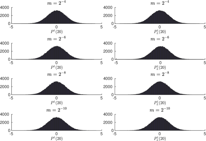
Figure 2. (Left column) histogram for the final time momentum of the heat bath dynamics for a series of $m$-values and (right column) corresponding histograms for the Langevin dynamics.

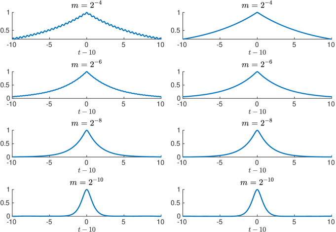
Figure 3. (Left column) heat bath dynamics auto-correlation function $\mathbb{E}[X^{1}(t)X^{1}(10)]$ for a series of $m$-values and (right column) corresponding Langevin dynamics auto-correlation functions $\mathbb{E}[X^{1}_{L}(t)X^{1}_{L}(10)]$.

Figure 4. (Left column) heat bath dynamics auto-correlation function $\mathbb{E}[P^{1}(t)P^{1}(10)]$ for a series of $m$-values and (right column) corresponding Langevin dynamics auto-correlation functions $\mathbb{E}[P^{1}_{L}(t)P^{1}_{L}(10)]$.

In addition to our above observations, we believe it would be of great interest to obtain numerical verification for the heat bath dynamics weak convergence rate $\mathcal{O}(m^{1/2})$ in (3.32). But, most likely due to computational constraints, we are unable to achieve this currently since even at the quite computationally demanding level of generating $M=200000$ heat bath dynamics sample paths, it seems that the sample error dominates errors pertaining to the parameter $m$.

References

- [1] A. Abdulle, G. Vilmart and K.C. Zygalakis. Long time accuracy of Lie–Trotter splitting methods for Langevin dynamics. SIAM Journal on Numerical Analysis, 53(1):1–16, 2015.
- [2] A.D. Baczewski and S.D. Bond. Numerical integration of the extended variable generalized langevin equation with a positive prony representable memory kernel. The Journal of chemical physics, 139(4):044107, 2013.
- [3] N. Bou-Rabee and H. Owhadi. Long-run accuracy of variational integrators in the stochastic context. SIAM Journal on Numerical Analysis, 48(1):278–297, 2010.
- [4] G.M. Dall’ara. Discreteness of the spectrum of Schrödinger operators with non-negative matrix valued potentials. Journal of Functional Analysis 268, no. 12 (2015) 3649-3679.
- [5] A. Brünger, C.L. Brooks III and M. Karplus. Stochastic boundary conditions for molecular dynamics simulations of st2 water. Chemical physics letters, 105(5):495–500, 1984.
- [6] G.W. Ford and M. Kac, On the quantum Langevin equation. J. Statist. Phys. 46 (1987), 803–810.
- [7] G.W. Ford, M. Kac and P. Mazur, Statistical mechanics of assemblies of coupled oscillators. J. Mathematical Phys. 6 (1965) 504–515.
- [8] M. Hairer, M. Hutzenthaler and A. Jentzen. Loss of regularity for Kolmogorov equations. The Annals of Probability 2015, Vol. 43, No. 2, 468–527.
- [9] E.J. Hall, M.A. Katsoulakis and L. Rey-Bellet. Uncertainty quantification for generalized Langevin dynamics. The Journal of chemical physics, 145(22):224108, 2016.
- [10] A. Kammonen, P. Plecháč, M. Sandberg and A. Szepessy. Canonical quantum observables for molecular systems approximated by ab initio molecular dynamics. Ann. Henri Poincar´e 19 (2018), 2727-2781.
- [11] D.P. Kroese, T. Taimre and Z.I. Botev. Handbook of Monte Carlo Methods, volume 706. John Wiley & Sons, 2013.
- [12] N.V. Krylov. Parabolic equations with VMO coefficients in Sobolev spaces with mixed norms. Journal of Functional Analysis 250 (2007) 521–558.
- [13] R. Kupferman. Fractional kinetics in Kac–Zwanzig heat bath models. Journal of statistical physics, 114(1-2):291–326, 2004.
- [14] P. Langevin. On the theory of Brownian movement. C.R.Acad. Sci. 146 530 (1908), (translation Am. J. Phys. 65 1079, 1997).
- [15] J.L. Lebowitz and E. Rubin. Dynamical study of Brownian motion. Phys. Rev. 131, 2381, 1963.
- [16] B. Leimkuhler and C. Matthews. Molecular Dynamics, volume 39 of Interdisciplinary Applied Mathematics. Springer, Cham, 2015.
- [17] T. Lelievre and G. Stoltz. Partial differential equations and stochastic methods in molecular dynamics. Acta Numerica, 25:681–880, 2016.
- [18] D. Marx and J. Hutter. Ab Initio Molecular Dynamics: Basic theory and advanced methods. Cambridge University Press (2009).
- [19] J.C. Mattingly, A.M. Stuart and D.J. Higham. Ergodicity for sdes and approximations: locally Lipschitz vector fields and degenerate noise. Stochastic processes and their applications, 101(2):185–232, 2002.
- [20] P.M. Mazur and I. Oppenheim. Molecular theory of Brownian motion. Physica 50 (1970) 241-258 8.
- [21] E.H. Müller, R. Scheichl and T. Shardlow. Improving multilevel Monte Carlo for stochastic differential equations with application to the Langevin equation. Proceedings of the Royal Society A: Mathematical, Physical and Engineering Sciences, 471(2176):20140679, 2015.
- [22] G.A. Pavliotis. Stochastic Processes and Applications. Diffusion processes, the Fokker-Planck and Langevin equations. Texts in Applied Mathematics, 60. Springer, New York (2014).
- [23] J-E. Shea and I. Oppenheim. Fokker-Planck Equation and Langevin Equation for one Brownian particle in a nonequilibrium bath. J. Phys. Chem. 1996, 100, 19035-19042.
- [24] R.D. Skeel and J.A. Izaguirre. An impulse integrator for Langevin dynamics. Molecular Physics, 100(24):3885–3891, 2002.
- [25] H.M. Stiepan and S. Teufel. Semiclassical approximations for Hamiltonians with operatorvalued symbols, Comm. Math. Phys. 320, no.3 (2013) 821-849.
- [26] R. Zwanzig. Nonequilibrium Statistical Mechanics, Oxford Univ. Press, New York (2001).
- [27] R. Zwanzig. Nonlinear generalized Langevin equations, J. Stat. Phys. 9 (1973) 215-220.
- [28] M. Zworski. Semiclassical Analysis, Providence, RI, American Mathematical Society (2012).