A Tensorized Transformer for Language Modeling

Abstract

Latest development of neural models has connected the encoder and decoder through a self-attention mechanism. In particular, Transformer, which is solely based on self-attention, has led to breakthroughs in Natural Language Processing (NLP) tasks. However, the multi-head attention mechanism, as a key component of Transformer, limits the effective deployment of the model to a resource-limited setting. In this paper, based on the ideas of tensor decomposition and parameters sharing, we propose a novel self-attention model (namely Multi-linear attention) with Block-Term Tensor Decomposition (BTD). We test and verify the proposed attention method on three language modeling tasks (i.e., PTB, WikiText-103 and One-billion) and a neural machine translation task (i.e., WMT-2016 English-German). Multi-linear attention can not only largely compress the model parameters but also obtain performance improvements, compared with a number of language modeling approaches, such as Transformer, Transformer-XL, and Transformer with tensor train decomposition.

1 Introduction

In NLP, Neural language model pre-training has shown to be effective for improving many tasks [15, 29]. Transformer [37] is based solely on the attention mechanism, and dispensing with recurrent and convolutional networks entirely. At present, this model has received extensive attentions and plays an key role in many neural language models, such as BERT [15], GPT [30] and Universal Transformer [13]. However, in Transformer based model, a lot of model parameters may cause problems in training and deploying these parameters in a resource-limited setting. Thus, the compression of large neural pre-training language models has been an essential problem in NLP research.

In literature, there are some compression methods [21, 40, 17] proposed. When the vocabulary is large, the corresponding weight matrices can be enormous. Tensorized embedding (TE) [21] uses the tensor-train [28] to compress the embedding layers in Transformer-XL [10], but has not compressed the attention layer. Recently, Block-Term Tensor Decomposition(BTD) [12] is used to compress recurrent neural networks (RNNs) [40]. Ye et al. [40] propose a compact flexible structure to deal with the large number of model parameters instead by high dimensional inputs in training recurrent neural networks (RNNs). This method greatly reduces the parameters of RNNs and improves their training efficiency. Still, the model only considers the input layer compression by the idea of low-rank approximation. On the other hand, some methods [17, 5] aim to develop a specific structure on its weight matrices and can reduce the parameters of the models. However, the new structure after compressing can not be integrated into the model [37].

In Transformer, the multi-head attention is a key part and it is constructed by a large number of parameters. Specifically, Ashish et.al [37] compute the attention function on a set of queries simultaneously, packed together into a matrix $Q$, while the keys and values are also packed together into matrices $K$ and $V$, respectively. The attention function then adopts a no-linear function $softmax$ over two matrices $Q$ and $K$. There are two challenges to find a high-quality compression method to compress the multi-head attention in Transformer.

First, the self-attention function in Transformer is a non-linear function, which makes it difficult to compress. In order to address this challenge, we first prove that the output of the attention function of the self-attention model [37] can be linearly represented by a group of orthonormal base vectors. Then, by initializing a low rank core tensor, we use Tucker-decomposition [35, 23] to reconstruct a new attention representation, where $Q$, $K$ and $V$ can be considered as factor matrices. In order to construct the multi-head mechanism and compress the model, we use the method of Block-Term Tensor Decomposition (BTD), which is a combination of CP decomposition [6] and Tucker decomposition [35]. The difference is that three factor matrices $Q,\leavevmode\nobreak\ K$ and $V$ are shared in constructing each $3$-order block tensor. This process can reduce many parameters.

The second challenge is that the attention model after compressing can not be directly integrated into the encoder and decoder framework of Transformer [37, 10]. In order to address this challenge, there are three steps as follows. First, the average of each block tensor can be computed; Second, multiple matrices can be given by tensor split. Third, the concatenation of these matrices can serve as the input to the next layer network in Transformer. After that, it can be integrated into the encoder and decoder framework of Transformer [37, 10] and trained end-to-end. Moreover, we also prove that the $3$-order tensor can reconstruct the scaled dot-product attention in Transformer by a sum on a particular dimension.

Our method combines two ideas which are the low-rank approximation and parameters sharing at the same time. Therefore, it achieves the higher compression ratios. Although the self-attention (i.e., scaled dot-product attention) in Transformer can be reconstructed, we do not consider reconstructing it and choose to split the $3$-order tensor (the output of Multi-linear attention) which is helpful for improving the accuracy in experiments.

Our major contributions of this paper are as follows:

• It is proved that the output of scaled dot-product attention (considering as a function) can be linearly represented by a group of orthonormal base vectors.

• A novel self-attention method, namely Multi-linear attention, is provided, which combines two compression ideas, parameters sharing and low-rank approximation, together.

• Multi-linear attention builds the strong connection between three factor matrices (pack a set of queries, keys and values, respectively ), enhancing the ability of capturing sufficient attention information. We also prove our model can reconstruct the scaled dot-product attention in the original Transformer.

In order to validate the benefits of our model, we test it on two NLP tasks, namely language modeling and neural machine translation. In our experiments, the multi-head attention can be replaced by the proposed model, namely multi-linear attention. We have observed that the standard Multi-head attention can be compressed with higher compression ratios on One-Billion dataset. As a result, we show that multi-linear attention not only considerably reduces the number of parameters, but also achieve promising experiments results, especially in language modeling tasks.

2 Preliminaries

Multi-linear attention is carried out in this paper. The analysis of Multi-linear attention relies on these concepts and results from the field of tensor decomositon and multi-head attention. We cover below in Section 2.1 basic background on Block-Term tensor decomposition [12]. Then, we describe in Section 2.2 multi-head attention [37].

2.1 Tensor and Block-Term Tensor Decomposition

Tensor We use the Euler script letter $\mathcal{A}$ to denote a tensor which can be thought of as a multi-array. Thereby a vector and a matrix are a $1$-order tensor and $2$-order tensor, respectively. The element in a $n$-order tensor is denoted as $\mathcal{A}_{d_{1},\ldots,d_{n}}$. In the geometric representation of a tensor, $3$-order tensor can be represented by a cube. After that, there is a related concept named $tensor\leavevmode\nobreak\ slice$ that will be used in this paper. Tensor and some other related concepts are showed in Supplementary Materials A.

Block-Term Tensor Decomposition (BTD) Block-Term tensor decomposition is a combination of CP decomposition [6] and Tucker decomposition [35]. Given a $n$-order tensor $\mathcal{A}\in\mathbb{R}^{d_{1}\times\ldots\times d_{n}}$. A high-order tensor can be decomposed into $P$ block terms by the method named BTD. ${\bullet}_{z}$ is denoted as the tenor-tensor product on the $z$-$th$ order [22] and $z\in\{1,\ldots,d\}$. Each term contains ${\bullet}_{z}$ between a core tensor $\mathcal{G}_{i}\in\mathbb{R}^{R_{1}\times\ldots\times R_{d}}$ and $d$ factor matrices $\mathcal{X}_{i}^{(k)}\in\mathbb{R}^{d_{k}\times R_{k}}$, where $i\in[1,P]$ and $k\in[1,d]$. The formulation of BTD decomposition is as follows:

$$\mathcal{A}=\sum_{i=1}^{P}\mathcal{G}_{i}{\bullet}_{1}\mathcal{X}_{i}^{(1)}{\bullet}_{2}\mathcal{X}_{i}^{2}{\bullet}_{3}\ldots{\bullet}_{d}\mathcal{X}_{i}^{(d)}$$ (1)

where $P$ is the CP rank, and $d$ is the Core-order. In our work, the tensor is $3$-order. Figure 1 demonstrates the example of how a $3$-order tensor $\mathcal{A}$ can be decomposed into $P$ block terms.

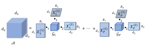
Figure 1: The representation of Block-Term tensor decomposition for a $3$-order tensor. $\mathcal{A}\in\mathbb{R}^{d_{1}\times d_{2}\times d_{3}}$ is a $3$-order tensor, and can be approximated by $P$ Tucker decomposition. $P$ is the CP rank, and $R_{1},R_{2},R_{3}$ are the Tucker rank, respectively. In this paper, we assume that $R$=$R_{1}$=$R_{2}$=$R_{3}$.

2.2 Multi-head Attention

In Transformer, the attention function is named as “Scaled Dot-Product Attention”. In practice, Transformer [37] processes query, keys and values as matrices $Q$, $K$, and $V$ respectively. The attention function can be written as follows:

$$Attention(Q,K,V)=softmax(\frac{QK^{T}}{\sqrt{d}})V$$ (2)

where $d$ is the number of columns of $Q$ and $K$. In these work [37, 15, 10], they all use the multi-head attention, as introduced in [37],

$$MultiHeadAttention(Q,K,V) =Concat(head_{1},\ldots,head_{k})W^{O}$$ (3)

$$where\leavevmode\nobreak\ head_{i} =Attention(QW^{Q}_{i},KW^{K}_{i},VW^{V}_{i})$$

where matrices $W^{Q}_{i}$ and $W^{K}_{i}\in\mathbb{R}^{d_{model}\times{d}}$, $W_{i}^{V}\in\mathbb{R}^{d_{model}\times{d}}$ and $W^{O}\in\mathbb{R}^{hd_{v}\times d_{model}}$. In practice, $d_{v}$ is equal to $d$. In this work [37], multiple groups of parameters ($W_{i}^{Q}$, $W_{i}^{K}$ and $W_{i}^{V}$) are used, which results in a large number of redundant parameters.

3 Tensorized Transformer

In this section, we first build a Single-block attention in Figure 2 (left) based on the Tucker decomposition, a low-rank decomposition method. In this process, we prove that the self-attention function in Transformer can be represented by a linear function, i.e., a linear combination representation of a set of basic vectors.

In order to compress the multi-head mechanism, we propose a multi-linear attention constructed by a Block-Term tensor decomposition. This attention uses the idea of parameters sharing, i.e., sharing factor matrices across multiple blocks, shown in Figure 2 (right). After that, the compression ratios and relatively lower complexity have been analyzed.

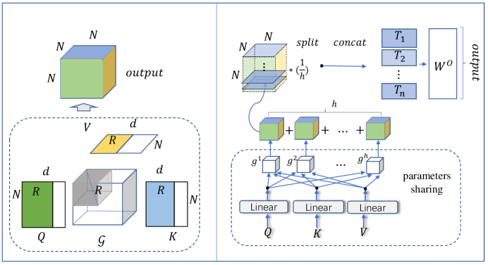
Figure 2: (left) Single-block attention using Tucker decomposition. (right) Multi-linear attention based on Block-Term tensor decomposition.

3.1 Single-block Attention by Tucker Decomposition

Before building the Single-block attention, it is necessary to propose the theorem 3.1. The theorem is closely related to attributes of Single-block attention function by Tucker decomposition [35].

Theorem 3.1.

Let $\bm{e}_{1},\ldots,\bm{e}_{n}$ be basis vectors from the vector space $S$. Assume that these vectors $\bm{e}_{1},\ldots,\bm{e}_{n}$ are linear independent and $Q$,$K$,$V$ can be linearly represented by this set of basis vectors. The output of the attention function in Eq. 2 can be represented by a linear combination of the set of these basis vectors.

$$Attention(Q,K,V)=(\bm{e}_{1},\ldots,\bm{e}_{n})M,$$ (4)

where $M\in\mathbb{R}^{n\times d}$ is a coefficient matrix, and $d$ is a dimension of these matrices (i.e., $Q,\leavevmode\nobreak\ K$, and $V$).

Proof.

The proof can be found in Supplementary Materials B. ∎

In Figure 2 (left), it is a schematic diagram about the Single-block attention. First, we assume that the query, key and value can be mapped into three factor matrices of which are composed of three groups of orthogonal basis vectors. Three factor matrices are $Q$, $K$ and $V$. After that, we can construct a new attention (i.e., Single-block attention) by initializing a $3$-order diagonal tensor (trainable) which is the $\mathcal{G}$. In Figure 2 (left), $R$ is the rank about the tensor, $N$ is the length of a sequence, and $d$ is the dimension of matrix. The function of Single-block attention can be computed based on Tucker-decomposition as follows:

$$Atten_{TD}(\mathcal{G};Q,K,V)= \mathcal{G}{\bullet}_{1}Q{\bullet}_{2}K{\bullet}_{3}V$$ (5)

$$= \sum_{i=1}^{I}\sum_{j=1}^{J}\sum_{m=1}^{M}\mathcal{G}_{ijm}Q_{i}\circ K_{j}\circ V_{m}$$

where $\mathcal{G}$ is a core tensor. $i,j$ and $m$ are the indexes of the core tensor. $\circ$ is the outer product. ${\bullet}_{z}$ is the same definition in Eq. 1. $Q_{i},K_{j}$ and $V_{k}$ are column vectors from matrices $Q,K$ and $V$, where $Q\in\mathbb{R}^{N\times d}$, $K\in\mathbb{R}^{N\times d}$ and $V\in\mathbb{R}^{N\times d}$, and $N$ is the length of a sequence. In practice, we set $I$=$J$=$M$=$R$. The core tensor $\mathcal{G}$ can be defined as follows,

$$\mathcal{G}_{ijm}=\left\{\begin{array}[]{lr}rand(0,1)&i=j=m\\ 0&otherwise\\ \end{array}\right.$$ (6)

where the $rand(0,1)$ is a random function, and the diagonal entries of core tensor $\mathcal{G}$ form the vector $\bm{g}$. Each entry $\bm{g}_{r}\in(0,1)$, $r\in\{1,\ldots,R\}$. We can consider $\bm{g}$ as the trainable weight. In experiments, we compute the weight vector by $softmax$ function (i.e., $softmax(\bm{g})$).

After that, the output of Single-block attention function is a $3$-order tensor which is given by linear computation. The Single-block attention (i.e., a $3$-order tensor with Tucker decomposition) can reconstruct the Scaled Dot-Product attention in Eq. 2 by the summing over the tensor according to the second index  (it can be seen as the coordinates in the vertical direction for a tensor), as proved in the following corollary. Note that in our model, we do not adopt the above reconstructing process. Instead, to obtain a new representation, we adopt the concat method after the tensor splitting (see Sec. 3.2). We will further show the compression ability of the Single-block attention in Sec. 3.3.

Corollary 1.

Under the same conditions as in Theorem 3.1 and the value of $N$ is equal to the value of $d$, Single-block attention representation Eq. 5 can reconstruct the Scaled Dot-Product attention in Eq. 2 by the summing over the tensor (i.e., the output of Single-block attention function) according to the second index. It holds that:

$$Attention(Q,K,V)_{i,m}=\sum_{j=1}^{N}Atten_{TD}(\mathcal{G};Q,K,V)_{i,j,m}$$ (7)

where $i$, $j$ and $m$ are the indices of the Single-block attention’s output (i.e., a 3-order tensor). $Atten_{TD}(\cdot)$ is the function of Single-block attention based on Tucker decomposition. $i$ and $m$ are the indices of outputs (i.e., a matrix) from Eq. 2.

Proof.

The proof can be found in Supplementary Materials C. ∎

3.2 Multi-Linear Attention by Block-Term Tensor Decomposition

In order to construct the multi-head mechanism and compress the parameters of multiple groups of mapping, we use a group of linear projections, and share the output from the linear projections. In Figure 2(right), the learned linear projection can map queries, keys and values to three matrices which are composed of basis vectors. After that, we use the Block-Term tensor decomposition to build multi-head mechanism. In our work, our model is named as Multi-linear attention, which can be formulated as follows:

$$MultiLinear(\mathcal{G};Q,K,V) =SplitConcat(\frac{1}{h}*({T}_{1}+\ldots+{T}_{h}))W^{O}$$ (8)

$$where\leavevmode\nobreak\ \leavevmode\nobreak\ {T_{j}} =Atten_{TD}(\mathcal{G}_{j};QW^{q},KW^{k},VW^{v})$$

where the core tensor $\mathcal{G}_{j}$ is a diagonal tensor, and the number of parameter in $\mathcal{G}_{j}$ is equal to the rank of core tensor, $j\in\{1,\ldots,h\}$. $\mathcal{G}$ is the set of the core tensors. $SplitConcat(\cdot)$ is a function which achieves the concatenation after splitting for a $3$-order tensor. Figure 2 (right) shows the basis idea about the multi-linear attention. The $W^{O}$ is the parameter matrix which is a full connection layer and correlated to the output of Multi-linear attention. $Atten_{TD}(\cdot)$ is the function of Single-block attention, which is a part of Multi-linear attention. $W^{q}$, $W^{K}$ and $W^{v}$ are the parameters matrices which are shared in constructing Multi-linear attention.

The Multi-linear attention is a compression model. After compressing the multi-head attention in Transformer, it is to achieve a Tensorized Transformer. The Multi-linear attention can be incorporated into Transformer architecture. A diagram which is about the incorporating of Multi-linear attention in partial Transformer structure is given in Supplementary Materials E.1.

3.3 Analysis of Compression and Complexity

Compression Our focus is on the compression of the multi-head mechanism in the multi-head attention of Transformer. Previous work [37] gets the multi-head attention by multiple groups of linear mappings. We use three linear mappings for matrices $Q$, $K$ and $V$, respectively. For the output of three mappings, we choose to share them which are considered as three factor matrices in reconstructing the Multi-linear attention. This process is shown in Figure 2 (left). $h$ is the number of heads in [37], and $d$ is the dimension of factor matrices. The compression ratios can be computed by $({3\times h\times d})/({3\times d+h})$. In practice, $h$ is normally set to $8$, $d$ is set to $512$. In this case, the compression ratios can achieve $8$. In other words, we can reduce almost $8$ times parameters in the attention layer. The details of the computing of compression ratios can be found in Supplementary Materials D. The Transformer also contains other network layers, such as Position-wise feed forward network and embedding layers et al. Therefore, for the compression ratios in whole Transformer, we can compare it by the analysis of experimental results for model parameters.

Complexity The time complexity of the attention function in Eq. 2 is $\mathcal{O}(N^{2}d)$, $N$ is the length of a sequence, and $d$ is the representation dimension. In Multi-linear attention, we can reorder the computations to receive the model complexity $\mathcal{O}(N^{3})$, where $N$ is also the length of the sequence. The minimum number of sequential operations in Multi-linear attention for different layers is approximately equal to the self-attention in Transformer [37].

4 Related Work

The field of language modeling has witnessed many significant advances. Different from the architectures of convolutional neural network (CNNs) and recurrent neural networks (RNNs) language modeling, the Transformer [37] and its variants [10, 15, 13] achieve excellent results in language modeling processing. Transformer networks have a potential of learning long-term dependency, but are limited by a fixed-length context in the setting of language modeling. Vaswani et al. [37] uses a segment-level recurrence mechanism and a novel positional encoding scheme to resolve this question. BERT [15] is a kind of bidirectional encoder representations from transformers. It is designed to pre-train deep bidirectional representation and obtains new SoTA on some NLP tasks. Although these methods have achieved great results, a large number of parameters make it difficult for the model to be trained in limited resources. Transformer fails to generalize in many simple tasks, e.g. copying string and logical inference [13]. Universal Transformers [13] propose a self-attentive recurrent sequence model which addresses this problem. This methods can increase the training speed. In their work, authors following weight sharing found in CNNs and RNNs, extend the Transformer with a simple form of weight sharing that strikes an effective balance between induces and model expressivity. This methods also uses a large number of parameters.

Therefore, it is very important to consider how to reduce the amount of memory and computing they need. As we know, existing model compression methods are mainly divided into parameter pruning and sharing [17], low rank approximation [31], knowledge transfer [5], and transferred convolutional filters [9]. Currently, tensor decomposition methods are used to decompose a high-order tensor, which can get different neural network language model structures [3, 1]. Besides, tensor decomposition methods which adopts the idea of low rank approximation in most cases, have been successfully applied to neural networks compression. For example, in literature [14, 19], researchers approximate a tensor by minimizing the reconstruction error of the original parameters on convolutional neural networks (CNNs). However, these approaches tend to accumulate errors when multiple layers are compressed sequentially, and the output feature maps deviate far from the original values with the increase of compressed layers. Our compression method uses the idea of parameters sharing in the constructing of attention layers, and the size of output is same as the output from self-attention in Transformer which can effectively avoid these problems. Tensorizing Neural Networks [27] have combined the idea of reshaping weights of fully-connected layers into high-dimensional tensors and representing them in Tensor Train format [28]. This approach was later extended to convolutional [16] and recurrent neural networks [38]. Recently, in these work [8, 36], researchers introduce efficient compression methods for the embedding and $softmax$ layers based on structured low rank matrix approximation. TT-embedding [21] aims to compression the larger embedding layer on Transformer-XL [10]. Sparse Transformer [2] adopts sparse techniques on the attention matrix and reduces its parameters. This work uses a sparse attention matrix by selecting the information on some positions in the attention matrix, but does not change the mechanism of the attention. Our method is different from these works, and combines two compression idea (low rank approximate and parameters sharing) to construct a tensorized Transformer.

In our work, we focus on the compression the multi-head attention in Transformer based the idea of parameters sharing. At the same time, we also combine low-rank approximate method to reduce parameters and computation complexity.

5 Experiments

Transformer is a versatile and powerful modeling tool and widely is used in various natural language process tasks. In order to verify the effectiveness of our method (i.e., Multi-linear attention) replacing multi-head attention in Transformer, we carry out two NLP tasks named language modeling (LM) and neural machine translation (NMT). Code for running experiments has been released, and the key code which is about our method can be found in Supplementary Materials F.

5.1 Language Modeling

Language modeling is the task of predicting the next word in a sentence. This task is to estimate the joint probability $p(s)$ of a sentence of tokens $s$=$(w_{1},\ldots,w_{n})$. The resulting models can be used to generate text or further fine-tuned to solve other NLP tasks [30]. In this paper, we employ the standard setting of predicting next token given the sequence of preceding tokens, based on the function $p(s)=p(w_{1})\prod_{i=2}^{n}p(w_{i}|w_{1},\ldots,w_{i-1})$. We chose three datasets in the order of small (i.e., PTB), medium (i.e., WikiText-103) and large (i.e., One-Billion). Models are evaluated based on Perplexity (PPL), which is the average per-word log-probability. The lower the PPL, the better the model is.

Specially, we take Transformer, the open source state-of-the art language modeling architecture, and replace the standard multi-head attention layers with our Multi-linear attention. Then, we test different model configurations on the PTB [26], WikiText-103 [25] and One-Billion Word benchmark [7] datasets and report the results in Table 1 and Table 2.

Table 1: Results (PPL) and model parameters with state-of-the-art results on One-Billion. Tensorized Transformer is our model. The core-1 is that the model use Single-block term tensor. Analogously, the core-2 is that two block term tensor is used.

Model	Params	Test PPL
RNN-1024+9 Gram [7]	20B	51.3
LSTM-2018-512 [20]	0.83B	43.7
GCNN-14 bottleneck [11]	–	31.9
LSTM-8192-1024+CNN Input [20]	1.04B	30.0
High-Budget MoE [34]	5B	28.0
LSTM+Mos [39]	113M	37.10
Transformer+adaptive input [4]	0.46B	23.7
Transformer-XL Base [10]	0.46B	23.5
Transformer-XL Large [10]	0.8B	21.8
Tensorized Transformer core-$1$	0.16B	20.5
Tensorized Transformer core-$2$	0.16B	19.5

Model	PTB			WikiText-103
	Params	Val PPL	Test PPL	Params	Val PPL	Test PPL
LSTM+augmented loss [18]	24M	75.7	48.7	–	–	48.7
Variational RHN [41]	23M	67.9	65.4	–	–	45.2
4-layer QRNN [24]	–	–	–	151M	–	33.0
AWD-LSTM-MoS [39]	22M	58.08	55.97	–	29.0	29.2
Transformer+adaptive input [4]	24M	59.1	57	247M	19.8	20.5
Transformer-XL-Base [10]	24M	56.72	54.52	151M	23.1	24.0
Transformer-XL-Large [10]	–	–	–	257M	–	18.3
Transformer-XL+TT [21]	18 M	57.9*	55.4*	130M	23.61*	25.70*
Sparse Transformer [2]	14M	74.0*	73.1*	174M	38.98*	40.23*
Tensorized Transformer core-$1$	12M	60.5	57.9	85.3M	22.7	20.9
Tensorized Transformer core-$2$	12M	54.25	49.8	85.3M	19.7	18.9

Table 2: Results and compression with state-of-the-art results on PTB and WikiText-103. ’$-$’ indicates no reported results in that setting, ’$*$’ indicates that the results is our own implementation.

5.2 Results and Details

PTB has $929k$ training tokens, $73k$ validation words, and $82k$ test words. The results is reported in Table 2. Similar to AWD-LSTM-MoS [39], we apply variational dropout and weight average to our model (i.e., Tensorized Transformer). In addition, we need to state that, our model only replaces the multi-head attention using Multi-linear attention structure, and the other structures remain the same. We compare the results of our model with other models. Our model achieves the comparable results with SoTA when the number of core tensor is equal to two. However, our model size (i.e, model parameters) reduces by nearly half comparing with Transformer and Transformer-XL.

WikiText-103 contains 267,735 unique tokens. The dataset is available word-level language modeling benchmark with long-term dependency. It contains 103M training tokens from $28k$ articles, with an average length of 3.6k tokens per article, which allows testing the ability of long-term dependency modeling. As shown in Table 2, our model get the perplexity of $18.9$, which is a comparable experimental result with the previous SoTA perplexity $18.3$ , which demonstrates the effectiveness of the proposed attention architecture.

The One-Billion Word benchmark is a large dataset derived from a news site. The dataset consists of $829,250,940$ tokens over a vocabulary of $793,471$ words. In this dataset, sentences are shuffled and hence the context is limited. Consequently, this dataset mainly tests the ability of modeling only short-term dependency. The comparison between Tensorized Transformer and the other methods are shown in Table 1. Although Tensorized Transformer is mainly designed to better compress Transformer or Transformer-XL model, it dramatically improves the single-model SoTA from 21.8 to 19.5. Specifically, Tensorized Transformer significantly outperforms a contemporary method using vanilla Transformers [37], suggesting that the advantage of the tensorized Transformer is also generalizable to modeling short sequences.

Table 2 and Table 1 show that our model get the lower PPL than other models in three datasets. An exciting observation is that our model has much fewer parameters. The model of Transformer-XL+TT [21] is a recent compression model with Tensor Train to compress the input embedding layers only. Sparse Transformer [2] uses the method of sparse attention matrix to compress Transformer model. The results in Table 2 show that compared with Transformer-XL+TT, our method has much fewer parameters, and better language modeling performance. These results verify that our model (i.e., Multi-linear attention) is effective in language modeling tasks, and has performed well for the model compression. Other details (such as hyperparameters and Hardware) can be found in Supplementary Materials E.

5.3 Neural Machine Translation

The goal is to map an input sequence $s=(x_{1},x_{2},\ldots,x_{n})$ representing a phrase in one language, to an output sequence $y=(y_{1},y_{2},\ldots,y_{m})$ representing the same phrase in a different language. In this task, we have trained the Transformer model [37] on WMT 2016 English-German dataset [33]. Sentences were tokenized using the SentencePiece . For our experiments, we have replaced each of the attention layers with Multi-linear attention in Encoder. For evaluation we used beam search with a beam size of 5 and length penalty $\alpha$=$0.6$. In this section, we only compared the results with Transformer [37]. Our results are summarized in Table 3. $*$ indicates that the result is our own implementation.

In Table 3, we select two baseline models. The Base-line [33] is first model in WMT 2016 English-German dataset. For the other baseline, we use the basic Transformer architecture [37]. The BLEU score is $34.5$ for the basic architecture. We carry out two Tensorized Transformer structures, namely core-1 and core-2 respectively. When Tensorized Transformer core-1 and core-2 are used, the BLEU scores are $34.10$ and $34.91$, which achieves better performance over Transformer. As for the reported model parameter size, our model uses less parameters.

Table 3: Results and compression with Transformer on WMT-16 English-to-German translation.

Model	Params	BLEU
Base-line [33]	–	26.8
Linguistic Input Featurec [32]	–	28.4
Attentional encoder-decoder + BPE [33]	–	34.2
Transformer [37]	52M	34.5*
Tensorized Transformer core-$1$	21M	34.10
Tensorized Transformer core-$2$	21.2M	34.91

5.4 Discussion

We have shown the results on language modeling and neural machine translation tasks using the Multi-linear attention. For the compression of the model parameters, although we report the parameters of the whole model structure, our method mainly considers the compression of multi-head attention but has not changed other layers in Transformer. Regarding the rationale for the improvements, in Corollary 1, we prove that the output of the original attention can be represented by summing over the 3-order tensor. In Figure 2, we use a concat function over these matrices from tensor splitting. The operation of concat can model all values in the 3-order tensor, and thus captures more information than sum operator. Another reason could be the alleviation of overfitting by reducing parameters. The overfitting will appear when the number of the core tensor is greater than 2. Besides, according to our experiments, relatively large dimensions of the word embedding can lead to overfitting, resulting in performance degradation. Therefore, our model requires a relatively small dimension of the embedding, compared with the original Transformer. In order for a more systematic evaluation, we report more experiments and analyses in Supplementary Materials E.4.

6 Conclusion and Further Work

We have proposed a novel self attention encoder layer, namely the Multi-linear attention, to compress the original multi-head attention and derive a novel encoding scheme. Our main contribution lies in a structure of Tensorized Transformer based on Block-Term tensor decomposition which is represented by the combination of a group of $3$-order tensors, with low-rank approximation and parameters sharing ideas adopted. Compared with existing Transformer based methods, our model achieved higher compression ratio and got better experimental results, particularly in language modeling task. These evidences imply that our method can potentially be further applied to more NLP tasks with limited resources.

In the future, we will continue to optimize the Tensorized Transformer framework and apply it in other NLP tasks. As we stated earlier, our model may suffer from overfitting when the number of cores is large in language modeling. In the future, we will explore the fundamental reasons that cause the problem and tackle them within the Tensorized Transformer framework.

7 Acknowledgement

This work is supported in part by the state key development program of China (grant No. 2017YFE0111900, 2018YFC0831704), Natural Science Foundation of China (grant No. 61772363, U1636203), and the European Unions Horizon 2020 research and innovation programme under the Marie SkodowskaCurie grant agreement No.721321.

Appendix A Tensor and Tensor Slice

As introduced in [42], a tensor and the tensor slice can be defined as follows.

Definition 1 (tensor).

Let $D_{1}$, $D_{2}$, $\ldots$, $D_{N}$$\in\mathbb{N}$ denote index upper bounds. A tensor $\mathcal{A}\in\mathbb{R}^{D_{1},\ldots,D_{N}}$ of order $N$ is an $N$-way array where elements $\mathcal{A}_{d_{1},d_{2},\ldots,d_{n}}$ are indexed by $d_{n}\in\{1,2,\ldots,D_{n}\}$ for $1\leq n\leq N$.

The concept of tensor slice is specified as:

Definition 2 (tensor slice).

A tensor slice is a two-dimensional section (fragment) of a tensor, obtained by fixing all indexes except for two indexes.

Appendix B Theorem 3.1

Let $\bm{e}_{1},\ldots,\bm{e}_{n}$ be basis vectors from the vector space $S$. Assume that these vectors $\bm{e}_{1},\ldots,\bm{e}_{n}$ are linear independent and $Q$,$K$,$V$ can be linearly represented by this set of basis vectors. The output of self-attention function in Eq. 2 (in the paper) can be represented by a linear combination of the set of these basis vectors.

$$Attention(Q,K,V)=(\bm{e}_{1},\ldots,\bm{e}_{n})M,$$ (9)

where $M\in\mathbb{R}^{n\times d}$ is a coefficient matrix, and $d$ is a dimension of these matrices (i.e., $Q,\leavevmode\nobreak\ K$, and $V$).

Proof.

If $Q$, $K$ and $V$ $\in$ Span($\bm{e}_{1},\ldots,\bm{e}_{n}$), the linear combination representation of matrices $Q$,$K$ and $V$ can be written as follows:

$$\left\{\begin{array}[]{lr}Q=\left(\bm{e}_{1},\bm{e}_{2},\ldots,\bm{e}_{n}\right)(\bm{\alpha}_{1},\bm{\alpha}_{2},\ldots,\bm{\alpha}_{d})\\ K=\left(\bm{e}_{1},\bm{e}_{2},\ldots,\bm{e}_{n}\right)(\bm{\beta}_{1},\bm{\beta}_{2},\ldots,\bm{\beta}_{d})\\ V=\left(\bm{e}_{1},\bm{e}_{2},\ldots,\bm{e}_{n}\right)(\bm{\xi}_{1},\bm{\xi}_{2},\ldots,\bm{\xi}_{d})\end{array}\right.$$ (10)

The self-attention function is written as follows [37]:

$$Attention(Q,K,V)=softmax(\frac{QK^{T}}{\sqrt{d}})V,$$ (11)

where $QK^{T}$ can be computed as follows:

$$QK^{T}=\left(\bm{e}_{1},\bm{e}_{2},\ldots,\bm{e}_{n}\right)(\bm{\alpha}_{1},\bm{\alpha}_{2},\ldots,\bm{\alpha}_{d})(\bm{\beta}_{1},\bm{\beta}_{2},\ldots,\bm{\beta}_{d})^{T}\left(\bm{e}_{1},\bm{e}_{2},\ldots,\bm{e}_{n}\right)^{T}$$ (12)

As a result, the input of $softmax$ function is a product of coefficient matrices $(\bm{\alpha}_{1},\ldots,\bm{\alpha}_{d})$ and $(\bm{\beta}_{1},\ldots,\bm{\beta}_{d})^{T}$. Then, we have

$$softmax(\frac{QK^{T}}{\sqrt{d}})=(\bm{e}_{1},\ldots,\bm{e}_{n})softmax(A/\sqrt{d})(\bm{e}_{1},\ldots,\bm{e}_{n})^{T}$$ (13)

where the matrix $A$ is equal to $(\bm{\alpha}_{1},\ldots,\bm{\alpha}_{d})(\bm{\beta}_{1},\ldots,\bm{\beta}_{d})^{T}$. Therefore, the attention representation can be written as follows:

$$softmax(\frac{QK^{T}}{\sqrt{d}})V =\left(\bm{e}_{1},\bm{e}_{2},\ldots,\bm{e}_{n}\right)softmax(A/\sqrt{d})(\bm{\xi}_{1},\bm{\xi}_{2},\ldots,\bm{\xi}_{d})$$ (14)

$$=\left(\bm{e}_{1},\bm{e}_{2},\ldots,\bm{e}_{n}\right)M$$

where the matrix $M$ is equal to $softmax(A/\sqrt{d})(\bm{\xi}_{1},\bm{\xi}_{2},\ldots,\bm{\xi}_{d})$. The $softmax(A/\sqrt{d})$ is to normalize the coefficient matrices of $Q$ and $K$. It turns out that the output of the attention function [37] can be represented by a linear combination of the set of basic vectors. ∎

After the proof, it is helpful to describe the basic idea. First, we consider that the self-attention function can be linearly represented by a set of orthogonal basis vectors, when the input of $softmax$ function is the product of two coefficient matrices, $(\bm{\alpha}_{1},\bm{\alpha}_{2},\ldots,\bm{\alpha}_{d})$ and $(\bm{\beta}_{1},\bm{\beta}_{2},\ldots,\bm{\beta}_{d})^{T}$, respectively. Second, in constructing the multi-head mechanism, the matrices of basis vectors $\left(\bm{e}_{1},\bm{e}_{2},\ldots,\bm{e}_{n}\right)$ can be shared.

Appendix C Corollary 1

Under the same conditions as in Theorem 3.1 and the value of $N$ is equal to the value of $d$, the Single-block attention representation Eq. $5$ (in the paper) can reconstruct the Scaled Dot-Product attention in Eq. $2$ (in the paper) by the summing over the tensor (i.e., the output of Single-block attention function) according to the second index. It holds that:

$$Attention(Q,K,V)_{i,m}=\sum_{j=1}^{N}Atten_{TD}(\mathcal{G};Q,K,V)_{i,j,m},$$ (15)

where $i$, $j$ and $m$ are the indices of the Single-block attention output (i.e., a 3-order tensor). $Atten_{TD}(\cdot)$ is the function of the Single-block attention based on Tucker decomposition. $i$ and $m$ are the indices of outputs (i.e., a matrix) from Eq. $2$ (in the paper).

Proof.

In Theorem 3.1, we have proved the results about the attention function can be represented by a linear combination of basis vectors. Therefore, we can represent the self-attention function in Eq. 2 (in the paper) by the form as follows:

$$Attention(Q,K,V)=\Theta QK^{T}V$$ (16)

where $\Theta$ is a normalization factor matrix, which can be used to replace the use of a $sofmax$ function. We assume that $\Theta$ contains all the non-zero elements of the core tensor $\mathcal{G}$. The self-attention in Eq. 2 (in the paper) can be re-written as follows:

$$X_{i,m}=\sum_{k=1}^{N}\sum_{r=1}^{R}{\Theta}_{i,m}Q_{i,r}K_{k,r}V_{k,m}$$ (17)

where $N$ is the length of a sentence, $X_{i,m}=Attention(Q,K,V)_{i,m}$ is the entry of the output from the self-attention, and $R$ is equal to $d$. Here the core tensor $\mathcal{G}$ is same as that in Eq. $7$ (in the paper). Then, the Single-block attention (a $3$-order tensor) can be represented as follows:

$$\mathcal{A}_{i,j,m}=\sum_{p}^{R}\sum_{q}^{R}\sum_{r}^{R}\mathcal{G}_{p,q,r}Q_{i,p}K_{j,p}V_{m,r}$$ (18)

where $\mathcal{A}$ is a $3$-order tensor, which is equal to $Atten_{TD}(\mathcal{G};Q,K,V)$. Accordingly, $\mathcal{A}_{i,j,m}$ is a entry in tensor $\mathcal{A}$ and is equal to ${Attention_{TD}}_{i,j,m}$ in Eq. 15. Next, we aim to prove Eq. 7 can be established. Therefore, we need to establish the relation between Eq. 18 and Eq. 17. Since the core tensor $\mathcal{G}$ is a special tensor (i.e., diagonal tensor), Eq. 18 can be written as follows:

$$\mathcal{A}_{i,j,m}=\sum_{r=1}^{R}\mathcal{G}_{r,r,r}Q_{i,r}K_{j,r}V_{m,r}$$ (19)

After that, we can compute the attention representation through adding to model $k$. For better understanding, we give the graph representation in Figure 3.

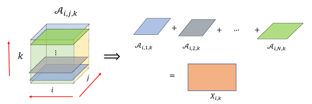
Figure 3: Tensor $\mathcal{A}$ is a $3$-order tensor, which represents the Single-block attention in the left. $\mathcal{A}_{i,j,k}$ is the entry of the tensor $\mathcal{A}$. In the right, the graph represents that the summing of tensor slices which is from the tensor splitting in index $j$. This graph can help us to understand the main content of corollary 1.

$$X_{i,m}=\sum_{r=1}^{R}\sum_{j=1}^{N}\mathcal{G}_{rrr}Q_{i,r}K_{j,r}V_{m,r}$$

The corollary then holds. ∎

Appendix D Compression Ratio about Multi-Linear Attention

In order to compute the compression ratio, we need to compare multi-linear attention with multi-head attention. The comparison chart has been given in Figure 4.

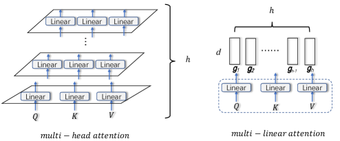
Figure 4: A diagram about a comparison of parameters between multi-linear attention and multi-head attention.

In Figure 4, each $Linear$ function in multi-head attention is about a weight matrix $W\in\mathbb{R}^{d_{model}\times d}$, and all weight matrices in multi-head attention are different. In multi-linear attention, three weight matrices are used and $h$ (a number) weight vectors are used. Through the analysis about Figure 4, the compression ratio is computed as follows.

$$\begin{split}compression\leavevmode\nobreak\ ratio=&\frac{3\times h\times d_{model}\times d}{3\times d_{model}\times d+h\times d}\\ =&\frac{3\times h\times d_{model}}{3\times d_{model}+h}\end{split}$$ (20)

In practice, $h$ is equal to $8$ and $d$ is equal to $512$. The compression ratio approximates $8$ in this case. In our work, the dimension of vector $\mathcal{G}_{r}$ is set as $R$ which is smaller than $d$, where $d$ is the dimension of attention matrix.

Low-rank Approximation for Model Compression In the paper, we have described that our method combines two compression ideas, namely low-rank approximation and parameters sharing. Parameters sharing can be understood through the description of Figure 4. In Multi-linear attention, the idea of low-rank decomposition also has the function of model compression. We have proved that the Single-block attention can re-construct an one-head self-attention in Transformer. In order to obtain the representation of a tensorized attention, we adopt the tensor splitting and the concat function. After that, we consider that each tensor slice from tensor splitting approximates the output of the self-attention function Eq. 2 (in the paper). When we only focus on the idea of low-rank approximation, the compression ratio can be computed by the form, $\frac{N\times d}{N\times N}$, where $N$ is the length of a sequence, $d$ is the dimension of a matrix (also namely hidden size). $N$ is smaller than $d$, normally.

Through combining the ideas of parameters sharing and low-rank approximation, by formally considering the rank $R$, the compression ratio of Multi-linear attention model can be computed as follows:

$$compression\leavevmode\nobreak\ ratio_{R}=\frac{3\times h\times d_{model}\times d}{3\times d_{model}\times d+R\times h},$$ (21)

where $R$ is the rank of the core tensor $\mathcal{G}$. The compression ratio will be larger when $R$ is smaller. This $compression\leavevmode\nobreak\ ratio_{R}$ is the compression ratio associated with $R$. $R$ need to be set in practice. In experiments, $R$ can be set to $18$, which is smaller than $d_{model}$.

Appendix E Experiment

E.1 Partial Structure about Tensorized Transformer

in the paper, the multi-linear attention is proposed. In order to show that the process of incorporating multi-linear attention into Transformer, Figure 5 gives out some information about the structure.

E.2 Experimental Details in Language Modeling

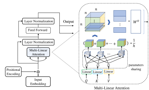
Figure 5: A diagram which is about the incorporating of multi-linear attention in partial Transformer structure. The parameters are shared in the constructing of each single-block attention.

Now, we report some details of experiments as a relevant supplementary material. Firstly, we use three weight matrices $W^{q}$,$W^{k}$ and $W^{v}$ to linearly project the queries, keys and values. The outputs from the linear projections can be shared by $h$ times, where $h$ is the number of core tensors in our background (i.e., core-1($h$=$1$), core-2($h$=$2$)). We use Block Term Tensor decomposition (BTD) to construct a new representation, namely Multi-linear attention, which is a $3$-order tensor. For incorporating the proposed attention into the architecture of Transformer, we split the $3$-order tensor, and then concat each matrix from the tensor. For other layers, we use the same structure as vanilla-Transformer.

Hardware

We trained our model on one machine with 2 NVIDIA P40 GPUs. For our base models, the hyperparameters are described in Table 4. In addition, we set the $dropout$=$0.3$ in all datasets. The model is trained using $30$ epochs in three datasets (PTB, WikiText-103 and One-Billion).

Table 4: The hyperparameters in the Tensorized Transformers model

Datasets	$d_{head}$	$d_{ff}$	h	L	$d_{k}$	$d_{v}$	Test PPL
PTB	256	2100	2	3	40	40	49.8
WikiText-103	256	2100	2	6	40	40	18.9
One-Billion	1024	2100	2	6	40	40	19.5

Optimizer We used the Adam optimizer and vary the learning rate over the course of training. The vary formula [37] is followed in our work. We also used the $warmup\_steps=4000$. Label Smoothing is employed with the value $\epsilon$=$0.1$.

E.3 Experiment Details in Neural Machine Translation

The Tensorized Transformer also has been applied to Neural Machine Translation task. In this experiment, we use the same setup with Transformer [37], and replace the multi-head attention with the proposed multi-linear attention in the encoder structure. In the decoder structure, we still use the multi-head attention for verifying the effectiveness of encoding a sentence. The model is trained in 1 NVIDA P40 GPUs.

E.4 Experimental comparison

For a more detailed comparison, we design these experiments as follows. In this section, we mainly show the experimental results on two language modeling datasets, i.e., PTB and WikiText-103. We show the value of perplexity, as well as FLOPs correspondingly.

Model	PTB			WikiText-103
	Params	FLOPS	Test PPL	Params	FLOPS	Test PPL
Transformer-XL [10]	24M	11.5B	59.1	257M	996.5B	18.3
Tensorized Transformer	24M	5.4B	52.7	257M	312.0B	21.2
Transformer-XL [10]	–	–	–	151M	126.5B	24.0
Tensorized Transformer	–	–	–	151M	83.4B	18.8
Transformer-XL [10]	12M	4.5B	87.8	85.5M	22.0B	34.8
Tensorized Transformer	12M	0.75B	57.9	85.5M	17.3B	20.9

Table 5: Experimental comparisons on PTB and WikiText-103.

Table 6: The same hyperparameters in Tensorized Transformers and Transformer-XL, $N$ is the length of sequence, and $L$ is the number of layers.

Datasets	Model	$d_{head}$	$d_{model}$	$N$	$L$	dropout	Test PPL
PTB	Transformer-XL	40	256	30	3	0.3	81.2
PTB	Tensorized Transformer	40	256	30	3	0.3	50.2
WikiText-103	Transformer-XL	40	256	80	6	0.1	34.86
WikiText-103	Tensorized Transformer	40	256	80	6	0.1	19.9
One-Billion	Transformer-XL	40	1024	100	6	0.1	43.6
One-Billion	Tensorized Transformer	40	1024	100	6	0.1	26.7

To further compare the experimental results under the same size of parameters between Tensorized Transformer and the baseline model (i.e., Transformer-XL), we add some experiments in Table 5. In our paper, we use the Tensorized Transformer of 12M on PTB dataset and the Tensorized Transformer of 85.5M on WikiText-103 dataset. To achieve the same size, i.e., 12M for Transformer-XL on PTB, we can reduce the dimensions of $Q,K,V$ from $40$ to $26$. To achieve Transformer-XL of 85.5M, we reduce the dimensions of word embedding from $512$ to $256$. The experimental results are shown in Table 5. Our model gets better results and the lower FLOPS than Transformer-XL.

On the other hand, we can also increase the parameters of Tensorized Transformer to reach the parameters reported by Transformer-XL on PTB and WikiText-103 datasets. On PTB dataset, we can increase the number of layers from $3$ to $7$ to get the Tensorized Transformer of 24M. On WikiText-103 dataset, we increase the number of layers from $6$ to $11$ and the length of sequence from $80$ to $120$ to get the Tensorized Transformer of 257M. We can increase the number of layers from $6$ to $8$ and the length of sequence from $80$ to $100$ to get the Tensorized Transformer of 151M. After that, Tensorized Transformer achieves better results and lower FLOPS than Transformer-XL. These results are shown in Table 5.

In addition, we also carry out experiments when Transformer-XL has the same hyperparameters with Tensorized Transformer. Experimental results are shown in Table 6. Table 6 shows that our model can get the better results than Transformer-XL. Besides, on two datasets (i.e., PTB and WiliText-103), we also try to train our model (Tensorized Transformer) using larger dimension of word embedding (i.e., $d_{model}$). If $d_{model}$ is larger than $256$ on PTB dataset and larger than $512$ on WikiText-103 dataset, the overfitting will occur. For the overfitting problem, we will investigate it in our future work.

Appendix F Partial Code

The project have been achieved by pytorch. In this section, we give the partial code which is about our methods, i.e., Sing-block attention and Multi-linear attention. First, the class of Single-block attention is given as follows.

⬇

import torch

import torch.nn as nn

import torch.nn.init as init

import numpy as np

class SingleBlockAttention(nn.Module):

’’’Single block attention’’’

def __init__(self, Rank):

super(SingleBlockAttention, self).__init__()

self.softmax = nn.Softmax()

self.R = Rank

def forward(self, q, k, v, mb_size,d):

self.core = nn.Parameter(torch.FloatTensor(np.random.rand(self.R)))

N = v.size(1)

self.core = self.softmax(self.R)

core_tensor = torch.zeros(N,d,N).cuda()

for i in range(self.R):

cores_tensor[i][i][i] = self.core[i]

full_matrixs = []

for i in range(mb_size):

full_matrix_1 = torch.einsum(’pqk, ip,jq,kr->ijr’, [core_tensor, q[i], k[i], v[i]]).contiguous()

full_matrixs.append(torch.sum(full_matrix_1, dim=1))

output = torch.stack(full_matrixs).cuda().float()

return output

Each Single block attention is a component of Multi-linear attention. Based on the Single block attention, the Multi-linear attention can be given as follows.

⬇

class MultiLinearAttention(nn.Module):

’’’ MultiLinearAttention ’’’

def __init__(self, h, Rank, d, dropout=0.1):

super(MultiLinearAttention, self).__init__()

self.n_head = h # h is equal to 2 in our model

self.d_k = d

self.d_v = d

self.w_q = nn.Parameter(torch.FloatTensor(d_model, d_k))

self.w_k = nn.Parameter(torch.FloatTensor(d_model, d_k))

self.w_v = nn.Parameter(torch.FloatTensor(d_model, d_v))

self.Tattention = SingleCoreAttention(Rank)

self.layer_norm = LayerNormalization(Rank)

self.proj = Linear(self.n_head*d, Rank)

self.dropout = nn.Dropout(dropout)

init.xavier_normal_(self.w_q)

init.xavier_normal_(self.w_k)

init.xavier_normal_(self.w_v)

def forward(self, q, k, v):

d_k, d_v = self.d_k, self.d_v

n_head = self.n_head

residual = q

mb_size, len_q, d_model = q.size()

mb_size, len_k, d_model = k.size()

mb_size, len_v, d_model = v.size()

q_s = q.repeat(1, 1).view(-1, d_model)

k_s = k.repeat(1, 1).view(-1, d_model)

v_s = v.repeat(1, 1).view(-1, d_model)

if n_head > 1:

output_1 = self.Tattention(q_s, k_s, v_s, mb_size,d_v)

output_2 = self.Tattention(q_s, k_s, v_s, mb_size,d_v)

output = (output_1+output_2)*0.5

else:

ouput = self.Tattention(q_s, k_s, v_s, mb_size,d_v)

# project back to residual size

outputs = self.proj(outputs)

outputs = self.dropout(outputs)

return self.layer_norm(outputs + residual)

References

- [1] Peng Zhang, Zhan Su, Lipeng Zhang, Benyou Wang, and Dawei Song. A quantum many-body wave function inspired language modeling approach. In Proceedings of the 27th ACM International Conference on Information and Knowledge Management, pages 1303–1312. ACM, 2018.
- [2] Alec Radford Rewon Child, Scott Gray and Ilya Sutskever. Generating long sequences with sparse transformer. arXiv preprint arXiv:1904.10509, 2019.
- [3] Lipeng Zhang, Peng Zhang, Xindian Ma, Shuqin Gu, Zhan Su, and Dawei Song. A generalized language model in tensor space. arXiv preprint arXiv:1901.11167, 2019.
- [4] Alexei Baevski and Michael Auli. Adaptive input representations for neural language modeling. arXiv preprint arXiv:1809.10853, 2018.
- [5] Cristian Bucilu, Rich Caruana, and Alexandru Niculescu-Mizil. Model compression. In Proceedings of the 12th ACM SIGKDD international conference on Knowledge discovery and data mining, pages 535–541. ACM, 2006.
- [6] J Douglas Carroll and Jih-Jie Chang. Analysis of individual differences in multidimensional scaling via an n-way generalization of “eckart-young” decomposition. Psychometrika, 35(3):283–319, 1970.
- [7] Ciprian Chelba, Tomas Mikolov, Mike Schuster, Qi Ge, Thorsten Brants, Phillipp Koehn, and Tony Robinson. One billion word benchmark for measuring progress in statistical language modeling. Computer Science, 2013.
- [8] Patrick Chen, Si Si, Yang Li, Ciprian Chelba, and Cho-Jui Hsieh. Groupreduce: Block-wise low-rank approximation for neural language model shrinking. In Advances in Neural Information Processing Systems, pages 10988–10998, 2018.
- [9] Taco Cohen and Max Welling. Group equivariant convolutional networks. In International conference on machine learning, pages 2990–2999, 2016.
- [10] Zihang Dai, Zhilin Yang, Yiming Yang, William W Cohen, Jaime Carbonell, Quoc V Le, and Ruslan Salakhutdinov. Transformer-xl: Attentive language models beyond a fixed-length context. arXiv preprint arXiv:1901.02860, 2019.
- [11] Yann N Dauphin, Angela Fan, Michael Auli, and David Grangier. Language modeling with gated convolutional networks. In Proceedings of the 34th International Conference on Machine Learning-Volume 70, pages 933–941. JMLR. org, 2017.
- [12] Lieven De Lathauwer. Decompositions of a higher-order tensor in block terms—part ii: Definitions and uniqueness. SIAM Journal on Matrix Analysis and Applications, 30(3):1033–1066, 2008.
- [13] Mostafa Dehghani, Stephan Gouws, Oriol Vinyals, Jakob Uszkoreit, and Łukasz Kaiser. Universal transformers. Published at ICLR2019, 2018.
- [14] Emily L Denton, Wojciech Zaremba, Joan Bruna, Yann LeCun, and Rob Fergus. Exploiting linear structure within convolutional networks for efficient evaluation. In Advances in neural information processing systems, pages 1269–1277, 2014.
- [15] Jacob Devlin, Ming-Wei Chang, Kenton Lee, and Kristina Toutanova. Bert: Pre-training of deep bidirectional transformers for language understanding. 2018.
- [16] Timur Garipov, Dmitry Podoprikhin, Alexander Novikov, and Dmitry Vetrov. Ultimate tensorization: compressing convolutional and fc layers alike. arXiv preprint arXiv:1611.03214, 2016.
- [17] Song Han, Jeff Pool, John Tran, and William Dally. Learning both weights and connections for efficient neural network. In Advances in neural information processing systems, pages 1135–1143, 2015.
- [18] Hakan Inan, Khashayar Khosravi, and Richard Socher. Tying word vectors and word classifiers: A loss framework for language modeling. arXiv preprint arXiv:1611.01462, 2016.
- [19] Max Jaderberg, Andrea Vedaldi, and Andrew Zisserman. Speeding up convolutional neural networks with low rank expansions. In Proceedings of the British Machine Vision Conference. BMVA Press, 2014.
- [20] Rafal Jozefowicz, Oriol Vinyals, Mike Schuster, Noam Shazeer, and Yonghui Wu. Exploring the limits of language modeling. arXiv preprint arXiv:1602.02410, 2016.
- [21] Valentin Khrulkov, Oleksii Hrinchuk, Leyla Mirvakhabova, and Ivan Oseledets. Tensorized embedding layers for efficient model compression. arXiv preprint arXiv:1901.10787, 2019.
- [22] Tamara G Kolda and Brett W Bader. Tensor decompositions and applications. SIAM review, 51(3):455–500, 2009.
- [23] Guangxi Li, Jinmian Ye, Haiqin Yang, Di Chen, Shuicheng Yan, and Zenglin Xu. Bt-nets: simplifying deep neural networks via block term decomposition. arXiv preprint arXiv:1712.05689, 2017.
- [24] Stephen Merity, Nitish Shirish Keskar, and Richard Socher. An analysis of neural language modeling at multiple scales. arXiv preprint arXiv:1803.08240, 2018.
- [25] Stephen Merity, Caiming Xiong, James Bradbury, and Richard Socher. Pointer sentinel mixture models. arXiv preprint arXiv:1609.07843, 2016.
- [26] Tomáš Mikolov, Anoop Deoras, Stefan Kombrink, Lukáš Burget, and Jan Černockỳ. Empirical evaluation and combination of advanced language modeling techniques. In Twelfth Annual Conference of the International Speech Communication Association, 2011.
- [27] Alexander Novikov, Dmitrii Podoprikhin, Anton Osokin, and Dmitry P Vetrov. Tensorizing neural networks. In Advances in neural information processing systems, pages 442–450, 2015.
- [28] Ivan V Oseledets. Tensor-train decomposition. SIAM Journal on Scientific Computing, 33(5):2295–2317, 2011.
- [29] Matthew Peters, Mark Neumann, Mohit Iyyer, Matt Gardner, Christopher Clark, Kenton Lee, and Luke Zettlemoyer. Deep contextualized word representations. In Proceedings of the 2018 Conference of the North American Chapter of the Association for Computational Linguistics: Human Language Technologies, Volume 1 (Long Papers), pages 2227–2237, 2018.
- [30] Alec Radford, Karthik Narasimhan, Tim Salimans, and Ilya Sutskever. Improving language understanding by generative pre-training. URL https://s3-us-west-2. amazonaws. com/openai-assets/research-covers/languageunsupervised/language understanding paper. pdf, 2018.
- [31] Tara N Sainath, Brian Kingsbury, Vikas Sindhwani, Ebru Arisoy, and Bhuvana Ramabhadran. Low-rank matrix factorization for deep neural network training with high-dimensional output targets. In 2013 IEEE international conference on acoustics, speech and signal processing, pages 6655–6659. IEEE, 2013.
- [32] Rico Sennrich and Barry Haddow. Linguistic input features improve neural machine translation. arXiv preprint arXiv:1606.02892, 2016.
- [33] Rico Sennrich, Barry Haddow, and Alexandra Birch. Edinburgh neural machine translation systems for wmt 16. arXiv preprint arXiv:1606.02891, 2016.
- [34] Noam Shazeer, Azalia Mirhoseini, Krzysztof Maziarz, Andy Davis, Quoc Le, Geoffrey Hinton, and Jeff Dean. Outrageously large neural networks: The sparsely-gated mixture-of-experts layer. arXiv preprint arXiv:1701.06538, 2017.
- [35] Ledyard R Tucker. Some mathematical notes on three-mode factor analysis. Psychometrika, 31(3):279–311, 1966.
- [36] Ehsan Variani, Ananda Theertha Suresh, and Mitchel Weintraub. West: Word encoded sequence transducers. arXiv preprint arXiv:1811.08417, 2018.
- [37] Ashish Vaswani, Noam Shazeer, Niki Parmar, Jakob Uszkoreit, Llion Jones, Aidan N Gomez, Łukasz Kaiser, and Illia Polosukhin. Attention is all you need. In Advances in neural information processing systems, pages 5998–6008, 2017.
- [38] Yinchong Yang, Denis Krompass, and Volker Tresp. Tensor-train recurrent neural networks for video classification. In Proceedings of the 34th International Conference on Machine Learning-Volume 70, pages 3891–3900. JMLR. org, 2017.
- [39] Zhilin Yang, Zihang Dai, Ruslan Salakhutdinov, and William W Cohen. Breaking the softmax bottleneck: A high-rank rnn language model. arXiv preprint arXiv:1711.03953, 2017.
- [40] Jinmian Ye, Linnan Wang, Guangxi Li, Di Chen, Shandian Zhe, Xinqi Chu, and Zenglin Xu. Learning compact recurrent neural networks with block-term tensor decomposition. In Proceedings of the IEEE Conference on Computer Vision and Pattern Recognition, pages 9378–9387, 2018.
- [41] Barret Zoph and Quoc V Le. Neural architecture search with reinforcement learning. arXiv preprint arXiv:1611.01578, 2016.
- [42] Andrzej Cichocki, Rafal Zdunek, Anh Huy Phan, and Shun-ichi Amari. Nonnegative matrix and tensor factorizations: applications to exploratory multi-way data analysis and blind source separation. John Wiley & Sons, 2009.