Cascade R-CNN: High Quality Object Detection and Instance Segmentation

Abstract

In object detection, the intersection over union (IoU) threshold is frequently used to define positives/negatives. The threshold used to train a detector defines its quality. While the commonly used threshold of 0.5 leads to noisy (low-quality) detections, detection performance frequently degrades for larger thresholds. This paradox of high-quality detection has two causes: 1) overfitting, due to vanishing positive samples for large thresholds, and 2) inference-time quality mismatch between detector and test hypotheses. A multi-stage object detection architecture, the Cascade R-CNN, composed of a sequence of detectors trained with increasing IoU thresholds, is proposed to address these problems. The detectors are trained sequentially, using the output of a detector as training set for the next. This resampling progressively improves hypotheses quality, guaranteeing a positive training set of equivalent size for all detectors and minimizing overfitting. The same cascade is applied at inference, to eliminate quality mismatches between hypotheses and detectors. An implementation of the Cascade R-CNN without bells or whistles achieves state-of-the-art performance on the COCO dataset, and significantly improves high-quality detection on generic and specific object detection datasets, including VOC, KITTI, CityPerson, and WiderFace. Finally, the Cascade R-CNN is generalized to instance segmentation, with nontrivial improvements over the Mask R-CNN. To facilitate future research, two implementations are made available at https://github.com/zhaoweicai/cascade-rcnn (Caffe) and https://github.com/zhaoweicai/Detectron-Cascade-RCNN (Detectron).

1 Introduction

Object detection is a complex problem, requiring the solution of two tasks. First, the detector must solve the recognition problem, distinguishing foreground objects from background and assigning them the proper object class labels. Second, the detector must solve the localization problem, assigning accurate bounding boxes to different objects. An effective architecture for the solution of the two tasks, on which many of the recently proposed object detectors are based, is the two-stage R-CNN framework [22, 21, 47, 37]. This frames detection as a multi-task learning problem that combines classification, to solve the recognition problem, and bounding box regression, to solve localization.

Despite the success of this architecture, the two problems can be difficult to solve accurately. This is partly due to the fact that there are many “close” false positives, corresponding to “close but not correct” bounding boxes. An effective detector must find all true positives in an image, while suppressing these close false positives. This requirement makes detection more difficult than other classification problems, e.g. object recognition, where the difference between positives and negatives is not as fine-grained. In fact, the boundary between positives and negatives must be carefully defined. In the literature, this is done by thresholding the intersection over union (IoU) score between candidate and ground truth bounding boxes. While the threshold is typically set at the value of $u=0.5$, this is a very loose requirement for positives. The resulting detectors frequently produce noisy bounding boxes, as shown in Fig. 1 (a). Hypotheses that most humans would consider close false positives frequently pass the $IoU\geq{0.5}$ test. While training examples assembled under the $u=0.5$ criterion are rich and diverse, they make it difficult to train detectors that can effectively reject close false positives.

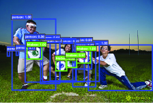
(a) Detection of $u=0.5$

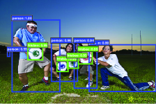
(b) Detection of $u=0.7$

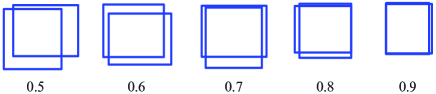
(c) Examples of increasing qualities

Figure 1: (a) and (b) detections by object detectors of increasing qualities, and (c) examples of increasing quality.

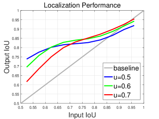
(a) Regressor

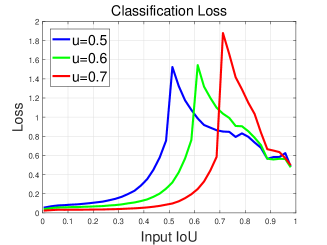
(b) Classifier

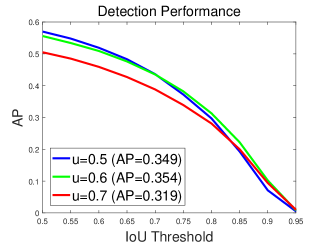
(c) Detector

Figure 2: Bounding box localization, classification loss and detection performance of object detectors of increasing IoU threshold $u$.

In this work, we define the quality of a detection hypothesis as its IoU with the ground truth, and the quality of a detector as the IoU threshold $u$ used to train it. Some examples of hypotheses of increasing quality are shown in Fig. 1 (c). The goal is to investigate the poorly researched problem of learning high quality object detectors. As shown in Fig. 1 (b), these are detectors that produce few close false positives. The starting premise is that a single detector can only be optimal for a single quality level. This is known in the cost-sensitive learning literature [12, 42], where the optimization of different points of the receiver operating characteristic (ROC) requires different loss functions. The main difference is that we consider the optimization for a given IoU threshold, rather than false positive rate.

Some evidence in support of this premise is given in Fig. 2, which presents the bounding box localization performance, classification loss and detection performance, respectively, of three detectors trained with IoU thresholds of $u=0.5,0.6,0.7$. Localization and classification are evaluated as a function of the detection hypothesis IoU. Detection is evaluated as a function of the IoU threshold, as in COCO [36]. Fig. 2 (a) shows that the three bounding box regressors tend to achieve the best performance for examples of IoU in the vicinity of the threshold used for detector training. Fig. 2 (c) shows a similar effect for detection, up to some overfitting for the highest thresholds. The detector trained with $u=0.5$ outperforms the detector trained with $u=0.6$ for low IoUs, underperforming it at higher IoUs. In general, a detector optimized for a single IoU value is not optimal for other values. This is also confirmed by the classification loss, shown in Fig. 2 (b), whose peaks are near the thresholds used for detector training. In general, the threshold determines the classification boundary where the classifier is most discriminative, i.e. has largest margin [6, 15].

The observations above suggest that high quality detection requires a close match between the quality of the detector and that of the detection hypotheses. The detector will only achieve high quality if presented with high quality proposals. This, however, cannot be guaranteed by simply increasing the threshold $u$ during training. On the contrary, as seen for the detector of $u=0.7$ in Fig. 2 (c), forcing a high value of $u$ usually degrades detection performance. We refer to this problem, i.e. that training a detector with higher threshold leads to poorer performance, as the paradox of high-quality detection. This problem has two causes. First, object proposal mechanisms tend to produce hypotheses distributions heavily imbalanced towards low quality. In result, the use of larger IoU thresholds during training exponentially reduces the number of positive training examples. This is particularly problematic for neural networks, which are very example intensive, making the “high $u$” training strategy very prone to overfitting. Second, there is a mismatch between the quality of the detector and that of the hypotheses available at inference time. Since, as shown in Fig. 2, high quality detectors are only optimal for high quality hypotheses, detection performance can degrade substantially for hypotheses of lower quality.

In this paper, we propose a new detector architecture, denoted as Cascade R-CNN, that addresses these problems, to enable high quality object detection. The new architecture is a multi-stage extension of the R-CNN, where detector stages deeper into the cascade are sequentially more selective against close false positives. As is usual for classifier cascades [54, 49], the cascade of R-CNN stages is trained sequentially, using the output of one stage to train the next. This leverages the observation that the output IoU of a bounding box regressor is almost always better than its input IoU, as can be seen in Fig. 2 (a), where nearly all plots are above the gray line. In result, the output of a detector trained with a certain IoU threshold is a good hypothesis distribution to train the detector of the next higher IoU threshold. This has some similarity to boostrapping methods commonly used to assemble datasets for object detection [54, 14]. The main difference is that the resampling performed by the Cascade R-CNN does not aim to mine hard negatives. Instead, by adjusting bounding boxes, each stage aims to find a good set of close false positives for training the next stage. The main outcome of this resampling is that the quality of the detection hypotheses increases gradually, from one stage to the next. In result, the sequence of detectors addresses the two problems underlying the paradox of high-quality detection. First, because the resampling operation guarantees the availability of a large number of examples for the training of all detectors in the sequence, it is possible to train detectors of high IoU without overfitting. Second, the use of the same cascade procedure at inference time produces a set of hypotheses of progressively higher quality, well matched to the increasing quality of the detector stages. This enables higher detection accuracies, as suggested by Fig. 2.

The Cascade R-CNN is quite simple to implement and trained end-to-end. Our results show that a vanilla implementation, without any bells and whistles, surpasses almost all previous state-of-the-art single-model detectors, on the challenging COCO detection task [36], especially under the stricter evaluation metrics. In addition, the Cascade R-CNN can be built with any two-stage object detector based on the R-CNN framework. We have observed consistent gains (of 2$\sim$4 points, and more under stricter localization metrics), at a marginal increase in computation. This gain is independent of the strength of the baseline object detectors, for all the models we have tested. We thus believe that this simple and effective detection architecture can be of interest for many object detection research efforts.

A preliminary version of this manuscript was previously published in [3]. After the original publication, the Cascade R-CNN has been successfully reproduced within many different codebases, including the popular Detectron [20], PyTorch, and TensorFlow, showing consistent and reliable improvements independently of implementation codebase. In this expanded version, we have extended the Cascade R-CNN to instance segmentation, by adding a mask head to the cascade, denoted as Cascade Mask R-CNN. This is shown to achieve non-trivial improvements over the popular Mask R-CNN [25]. A new and more extensive evaluation is also presented, showing that the Cascade R-CNN is compatible with many complementary enhancements proposed in the detection and instance segmentation literatures, some of which were introduced after [3], e.g. GroupNorm [56]. Finally, we further present the results of a larger set of experiments, performed on various popular generic/specific object detection datasets, including PASCAL VOC [13], KITTI [16], CityPerson [64] and WiderFace [61]. These experiments demonstrate that the paradox of high quality object detection applies to all these tasks, and that the Cascade R-CNN enables more effective high quality detection than previously available methods. Due to these properties, as well as its generality and flexibility, the Cascade R-CNN has recently been adopted by the winning teams of the COCO 2018 instance segmentation challenge, the OpenImage 2018 challenge, and the Wider Challenge 2018. To facilitate future research, we have released the code on two codebases, Caffe [31] and Detectron [20].

2 Related Work

Due to the success of the R-CNN [22] detector, which combines a proposal detector and a region-wise classifier, this two-stage architecture has become predominant in the recent past. To reduce redundant CNN computations, the SPP-Net [26] and Fast R-CNN [21] introduced the idea of region-wise feature extraction, enabling the sharing of the bulk of feature computations by object instances. The Faster R-CNN [47] then achieved further speeds-up by introducing a region proposal network (RPN), becoming the cornerstone of modern object detection. Later, some works extended this detector to address various problems of detail. For example, the R-FCN [8] proposed efficient region-wise full convolutions to avoid the heavy CNN computations of the Faster R-CNN; and the Mask R-CNN [25] added a network head that computes object masks to support instance segmentation. Some more recent works have focused on normalizing feature statistics [45, 56], modeling relations between instances [28], non maximum suppression (NMS) [1], and other aspects [50, 39].

Scale invariance, an important requisite for effective object detection, has also received substantial attention in the literature [2, 37, 52]. While natural images contain objects at various scales, the fixed receptive field size of the filters implemented by the RPN [47] makes it prone to scale mismatches. To overcome this, the MS-CNN [2] introduced a multi-scale object proposal network, by generating outputs at multiple layers. This leverages the different receptive field sizes of the different layers to produce a set of scale-specific proposal generators, which is then combined into a strong multi-scale generator. Similarly, the FPN [37] detects high-recall proposals at multiple output layers, with recourse to a scale-invariant feature representation by adding a top-down connection across feature maps of different network depths. Both the MS-CNN and FPN rely on a feature pyramid representation for multi-scale object detection. SNIP [52], on the other hand, recently revisited image pyramid in modern object detection. It normalizes the gradients from different object scales during training, such that the whole detector is scale-specific. Scale-invariant detection is achieved by using an image pyramid at inference.

One-stage object detection architectures have also become popular for their computational efficiency. YOLO [46] outputs very sparse detection results and enables real-time object detection, by forwarding the input image once through an efficient backbone network. SSD [40] detects objects in a way similar to the RPN [47], but uses multiple feature maps at different resolutions to cover objects at various scales. The main limitation of these detectors is that their accuracy is typically below that of two-stage detectors. The RetinaNet [38] detector was proposed to address the extreme foreground-background class imbalance of dense object detection, achieving results comparable to two-stage detectors. Recently, CornerNet [33] proposed to detect an object bounding box as a pair of keypoints, abandoning the widely used concept of anchors first introduced by the Faster R-CNN. This detector has achieved very good performance with the help of some training and testing enhancements. RefineDet [65] added an anchor refinement module to the single-shot SSD [40], to improve localization accuracy. This is somewhat similar to the cascaded localization implemented by the proposed Cascade R-CNN, but ignores the problem of high-quality detection.

(a) Faster R-CNN

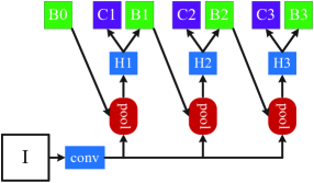
(b) Cascade R-CNN

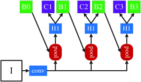
(c) Iterative BBox at inference

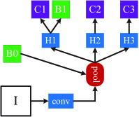
(d) Integral Loss

Figure 3: The architectures of different frameworks. “I” is input image, “conv” backbone convolutions, “pool” region-wise feature extraction, “H” network head, “B” bounding box, and “C” classification. “B0” is proposals in all architectures.

Some explorations in multi-stage object detection have also been proposed. The multi-region detector of [17] introduced iterative bounding box regression, where a R-CNN is applied several times to produce successively more accurate bounding boxes. [60, 19, 18] used a multi-stage procedure to generate accurate proposals, which are forwarded to an accurate model (e.g. Fast R-CNN). [62, 43] proposed an alternative procedure to localize objects sequentially. While this is similar in spirit to the Cascade-RCNN, these methods use the same regressor iteratively for accurate localization. On the other hand, [34, 44] embedded the classic cascade architecture of [54] in an object detection network. Finally, [7] iterated between the detection and segmentation tasks, to achieve improved instance segmentation.

Upon publication of the conference version of this manuscript, several works have pursued the idea behind Cascade R-CNN [32, 41, 55, 5]. [41, 55] applied it to single-shot object detectors, showing nontrivial improvements for high quality single-shot detection, for general objects and pedestrians, respectively. The IoU-Net [32] explored in greater detail high-quality localization, achieving some gains over the Cascade R-CNN by cascading more bounding box regression steps. [24] showed it is possible to achieve state-of-the-art object detectors without ImageNet pretraining, with a help of the Cascade R-CNN. These works show that the Cascade R-CNN idea is robust and applicable to various object detection architectures. This suggests that it should continue to be useful despite future advances in object detection.

3 High Quality Object Detection

In this section, we discuss the challenges of high quality object detection.

3.1 Object Detection

While the ideas proposed in this work can be applied to various detector architectures, we focus on the popular two-stage architecture of the Faster R-CNN [47], shown in Fig. 3 (a). The first stage is a proposal sub-network, in which the entire image is processed by a backbone network, e.g. ResNet [27], and a proposal head (“H0”) is applied to produce preliminary detection hypotheses, known as object proposals. In the second stage, these hypotheses are processed by a region-of-interest detection sub-network (“H1”), denoted as a detection head. A final classification score (“C”) and a bounding box (“B”) are assigned per hypothesis. The entire detector is learned end-to-end, using a multi-task loss with bounding box regression and classification components.

3.1.1 Bounding Box Regression

A bounding box $\textbf{b}=(b_{x},b_{y},b_{w},b_{h})$ contains the four coordinates of an image patch $\bf x$. Bounding box regression aims to regress a candidate bounding box b into a target bounding box g, using a regressor $f({\bf x},\textbf{b})$. This is learned from a training set $(\textbf{g}_{i},\textbf{b}_{i})$, by minimizing the risk

$${\cal R}_{loc}[f]=\sum_{i}L_{loc}(f({\bf x}_{i},\textbf{b}_{i}),\textbf{g}_{i}).$$ (1)

As in Fast R-CNN [21],

$$L_{loc}({\bf a},{\bf b})=\sum_{i\in\{x,y,w,h\}}smooth_{L_{1}}(a_{i}-b_{i})$$ (2)

where

$$smooth_{L_{1}}(x)=\left\{\begin{array}[]{cl}0.5x^{2},&\quad\textrm{$|x|<1$}\\ |x|-0.5,&\quad\textrm{otherwise,}\end{array}\right.$$ (3)

is the smooth $L_{1}$ loss function. To encourage invariance to scale and location, $smooth_{L_{1}}$ operates on the distance vector $\Delta=(\delta_{x},\delta_{y},\delta_{w},\delta_{h})$ defined by

$$\begin{array}[]{cl}\delta_{x}=(g_{x}-b_{x})/b_{w},\quad\delta_{y}=(g_{y}-b_{y})/b_{h}\\ \delta_{w}=\log(g_{w}/b_{w}),\quad\delta_{h}=\log(g_{h}/b_{h}).\end{array}$$ (4)

Since bounding box regression usually performs minor adjustments on b, the numerical values of (4) can be very small. This usually makes the regression loss much smaller than the classification loss. To improve the effectiveness of multi-task learning, $\Delta$ is normalized by its mean and variance, e.g. $\delta_{x}$ is replaced by

$$\delta_{x}^{\prime}=\frac{\delta_{x}-\mu_{x}}{\sigma_{x}}.$$ (5)

This is widely used in the literature [47, 2, 8, 37, 25].

3.1.2 Classification

The classifier is a function $h({\bf x})$ that assigns an image patch $\bf x$ to one of $M+1$ classes, where class $0$ contains background and the remaining classes the objects to detect. $h({\bf x})$ is a $M+1$-dimensional estimate of the posterior distribution over classes, i.e. $h_{k}({\bf x})=p(y=k|{\bf x})$, where $y$ is the class label. Given a training set $({\bf x}_{i},y_{i})$, it is learned by minimizing the classification risk

$${\cal R}_{cls}[h]=\sum_{i}L_{cls}(h({\bf x}_{i}),y_{i}),$$ (6)

where

$$L_{cls}(h({\bf x}),y)=-\log h_{y}({\bf x})$$ (7)

is the cross-entropy loss.

3.2 Detection Quality

Consider a ground truth object of bounding box ${\bf g}$ associated with class label $y$, and a detection hypothesis ${\bf x}$ of bounding box ${\bf b}$. Since a $\bf b$ usually includes an object and some amount of background, it can be difficult to determine if a detection is correct or not. This is usually addressed by the intersection over union (IoU) metric

$$IoU({\bf b},{\bf g})=\frac{{\bf b}\cap{\bf g}}{{\bf b}\cup{\bf g}}.$$ (8)

If the IoU is above a threshold $u$, the patch is considered an example of the class of the object of bounding box $\bf g$ and denoted “positive”. Thus, the class label of a hypothesis ${\bf x}$ is a function of $u$,

$$y_{u}=\left\{\begin{array}[]{cl}y,&\quad\textrm{$IoU({\bf b},{\bf g})\geq{u}$}\\ 0,&\quad\textrm{otherwise.}\end{array}\right.$$ (9)

If the IoU does not exceed the threshold for any object, $\bf x$ is assigned to the background and denoted “negative”.

Although there is no need to define positive/neagtive examples for the bounding box regression task, an IoU threshold $u$ is also required to select the set of samples

$$\mathcal{G}=\{(\textbf{g}_{i},\textbf{b}_{i})|IoU({\bf b}_{i},{\bf g}_{i})\geq{u}\}$$ (10)

used to train the regressor. While the IoU thresholds used for the two tasks do not have to be identical, this is usual in practice. Hence, the IoU threshold $u$ defines the quality of a detector. Large thresholds encourage detected bounding boxes to be tightly aligned with their ground truth counterparts. Small thresholds reward detectors that produce loose bounding boxes, of small overlap with the ground truth.

A main challenge of object detection is that, no matter the choice of threshold, the detection setting is highly adversarial. When $u$ is high, positives contain less background but it is difficult to assemble large positive training sets. When $u$ is low, richer and more diverse positive training sets are possible, but the trained detector has little incentive to reject close false positives. In general, it is very difficult to guarantee that a single classifier performs uniformly well over all IoU levels. At inference, since the majority of the hypotheses produced by a proposal detector, e.g. RPN [47] or selective search [53], have low quality, the detector must be more discriminant for lower quality hypotheses. A standard compromise between these conflicting requirements is to settle on $u=0.5$, which is used in almost all modern object detectors. This, however, is a relatively low threshold, leading to low quality detections that most humans consider close false positives, as shown in Fig. 1 (a).

3.3 Challenges to High Quality Detection

Despite the significant progress in object detection of the past few years, few works attempted to address high quality detection. This is mainly due to the following reasons.

First, evaluation metrics have historically placed greater emphasis on the low quality detection regime. For performance evaluation, an IoU threshold $u$ is used to determine whether a detection is a success ($IoU({\bf b},{\bf g})\geq{u}$) or failure ($IoU({\bf b},{\bf g})<u$). Many object detection datasets, including PASCAL VOC [13], ImageNet [48], Caltech Pedestrian[11], etc., use $u=0.5$. This is partly because these datasets were established a while ago, when object detection performance was far from what it is today. However, this loose evaluation standard is adopted even by relatively recent datasets, such as WiderFace [61], or CityPersons [64]. This is one of the main reasons why performance has saturated for many of these datasets. Others, such as COCO [36] or KITTI [16] use stricter evaluation metrics: average precision at $u=0.7$ for car in KITTI, and mean average precision across $u=[0.5:0.05:0.95]$ in COCO. While recent works have focused on these less saturated datasets, most detectors are still designed with the loose IoU threshold of $u=0.5$, associated with the low-quality detection regime. In this work, we show that there is plenty of room for improvement when a stricter evaluation metric, e.g. $u\geq{0.75}$, is used and that it is possible to achieve significant improvements by designing detectors specifically for the high quality regime.

Second, the design of high quality object detectors is not a trivial generalization of existing approaches, due to the paradox of high quality detection. To beat the paradox, it is necessary to match the qualities of the hypotheses generator and the object detector. In the literature, there have been efforts to increase the quality of hypotheses, e.g. by iterative bounding box regression [19, 18] or better RPN design [2, 37], and some efforts to increase the quality of the object detector, e.g. by using the integral loss on a set of IoU thresholds [63]. These attempts fail to guarantee high quality detection because they consider only one of the goals, missing the fact that the qualities of both tasks need to be increased simultaneously. On one hand, raising the quality of the hypotheses has little benefit if the detector remains of low quality, because the latter is not trained to discriminate high quality from low quality hypotheses. On the other, if only the detector quality is increased, there are too few high quality hypotheses for it to classify, leading to no detection improvement. In fact, because, as shown in Fig. 4 (left), the set of positive samples decreases quickly with $u$, a high $u$ detector is prone to overfitting. Hence, a high $u$ detector can easily overfit and perform worse than a low $u$ detector, as shown in Fig. 2 (c).

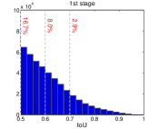
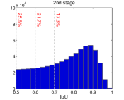
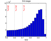
Figure 4: IoU histograms of training samples of each cascade stage. The distribution of the 1st stage is the RPN output. Shown in red are the percentage of positives for the corresponding IoU threshold.

4 Cascade R-CNN

In this section we introduce the Cascade R-CNN detector.

4.1 Architecture

The architecture of the Cascade R-CNN is shown in Fig. 3 (b). It is a multi-stage extension of the Faster R-CNN architecture of Fig. 3 (a). In this work, we focus on the the detection sub-network, simply adopting the RPN [47] of Fig. 3 (a) for proposal detection. However, the Cascade R-CNN is not limited to this proposal mechanism, other choices should be possible. As discussed in the section above, the goal is to increase the quality of hypotheses and detector simultaneously, to enable high quality object detection. This is achieved with a combination of cascaded bounding box regression and cascaded detection.

4.2 Cascaded Bounding Box Regression

High quality hypotheses can be easily produced during training, where ground truth bounding boxes are available, e.g. by sampling around the ground truth. The difficulty is to produce high quality proposals at inference, when ground truth is unavailable. This problem is addressed with resort to cascaded bounding box regression.

As shown in Fig. 2 (a), a single regressor cannot usually perform uniformly well over all quality levels. However, as is commonly done for pose regression [10] or face alignment [4, 58, 59], the regression task can be decomposed into a sequence of simpler steps. In the Cascade R-CNN detector, the idea is implemented with a cascaded regressor with the architecture of Fig. 3 (b). This consists of a cascade of specialized regressors

$$f({\bf x},\textbf{b})=f_{T}\circ{f}_{T-1}\circ\cdots\circ{f}_{1}({\bf x},\textbf{b}),$$ (11)

where $T$ is the total number of cascade stages. The key point is that each regressor $f_{t}$ is optimized for the bounding box distribution $\{\textbf{b}^{t}\}$ generated by the previous regressor, rather than the initial distribution $\{\textbf{b}^{1}\}$. In this way, the hypotheses are improved progressively.

This is illustrated in Fig. 5, which presents the distribution of the regression distance vector $\Delta=(\delta_{x},\delta_{y},\delta_{w},\delta_{h})$ at different cascade stages. Note that most hypotheses become closer to the ground truth as they progress through the cascade. There are also some hypotheses that fail to meet the stricter IoU criteria of the later cascade stages. These are declared outliers and eliminated. It should be noted that, as discussed in Section 3.1.1, $\Delta$ needs be mean/variance normalized, as in (5), for effective multi-task learning. The mean and variance statistics computed after this outlier removal step are used to normalize $\Delta$ at each cascade stage. Our experiments show that this implementation of cascaded bounding box regression generates hypotheses of very high quality at both training and inference.

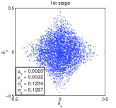
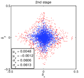
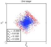
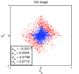
Figure 5: Distribution of the distance vector $\Delta$ of (4) (without normalization) at different cascade stages. Top: plot of $(\delta_{x},\delta_{y})$. Bottom: plot of $(\delta_{w},\delta_{h})$. Red dots are outliers for the increasing IoU thresholds of later stages, and the statistics shown are obtained after outlier removal.

4.3 Cascaded Detection

As shown in the left of Fig. 4, the initial hypotheses distribution produced by the RPN is heavily tilted towards low quality. For example, only 2.9% of examples are positive for an IoU threshold $u=0.7$. This makes it difficult to train a high quality detector. The Cascade R-CNN addresses the problem by using cascade regression as a resampling mechanism. This is inspired by Fig. 2 (a), where nearly all curves are above the diagonal gray line, showing that a bounding box regressor trained for a certain $u$ tends to produce bounding boxes of higher IoU. Hence, starting from examples $\{({\bf x}_{i},\textbf{b}_{i})\}$, cascade regression successively resamples an example distribution $\{({\bf x}^{\prime}_{i},\textbf{b}^{\prime}_{i})\}$ of higher IoU. This enables the sets of positive examples of the successive stages to keep a roughly constant size, even when the detector quality $u$ is increased. Figure 4 illustrates this property, showing how the example distribution tilts more heavily towards high quality examples after each resampling step.

At each stage $t$, the R-CNN head includes a classifier $h_{t}$ and a regressor $f_{t}$ optimized for the corresponding IoU threshold $u^{t}$, where $u^{t}>u^{t-1}$. These are learned with loss

$$L({\bf x}^{t},g)=L_{cls}(h_{t}({\bf x}^{t}),y^{t})+\lambda[y^{t}\geq{1}]L_{loc}(f_{t}({\bf x}^{t},\textbf{b}^{t}),\textbf{g}),$$ (12)

where $\textbf{b}^{t}=f_{t-1}({\bf x}^{t-1},\textbf{b}^{t-1})$, $\bf g$ is the ground truth object for ${\bf x}^{t}$, $\lambda=1$ the trade-off coefficient, $y^{t}$ is the label of ${\bf x}^{t}$ under the $u^{t}$ criterion, according to (9), $[\cdot]$ is the indicator function. Note that the use of $[\cdot]$ implies that the IoU threshold $u$ of bounding box regression is identical to that used for classification. This cascade learning has three important consequences for detector training. First, the potential for overfitting at large IoU thresholds $u$ is reduced, since positive examples become plentiful at all stages (see Fig. 4). Second, detectors of deeper stages are optimal for higher IoU thresholds. Third, because some outliers are removed as the IoU threshold increases (see Fig. 5), the learning effectiveness of bounding box regression increases in the later stages. This simultaneous improvement of hypotheses and detector quality enables the Cascade R-CNN to beat the paradox of high quality detection. At inference, the same cascade is applied. The quality of the hypotheses is improved sequentially, and higher quality detectors are only required to operate on higher quality hypotheses, for which they are optimal. This enables the high quality object detection results of Fig. 1 (b), as suggested by Fig. 2.

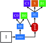
(a)

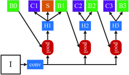
(b)

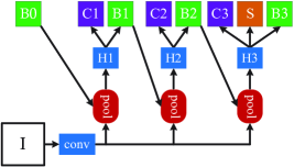
(c)

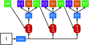
(d)

Figure 6: Architectures of the Mask R-CNN (a) and three Cascade Mask R-CNN strategies for instance segmentation (b)-(d). Beyond the definitions of Fig. 3, “S” denotes a segmentation branch. Note that segmentations branches do not necessarily share heads with the detection branch.

4.4 Differences from Previous Works

The Cascade R-CNN has similarities to previous works using iterative bounding box regression and integral loss for detection. There are, however, important differences.

Iterative Bounding Box Regression: Some works [17, 18, 27] have previously argued that the use of a single bounding box regressor $f$ is insufficient for accurate localization. These methods apply $f$ iteratively, as a post-processing step

$$f^{\prime}({\bf x},\textbf{b})=f\circ{f}\circ\cdots\circ{f}({\bf x},\textbf{b}),$$ (13)

that refines a bounding box b. This is called iterative bounding box regression and denoted as iterative BBox. It can be implemented with the inference architecture of Fig. 3 (c) where all heads are identical. Note that this is only for inference, as training is identical to that of a two-stage object detector, e.g. the Faster R-CNN of Fig. 3 (a) with $u=0.5$. This approaches ignores two problems. First, as shown in Fig. 2, a regressor $f$ trained at $u=0.5$ is suboptimal for hypotheses of higher IoUs. It actually degrades bounding box accuracy for IoUs larger than $0.85$. Second, as shown in Fig. 5, the distribution of bounding boxes changes significantly after each iteration. While the regressor is optimal for the initial distribution it can be quite suboptimal after that. Due to these problems, iterative BBox requires a fair amount of human engineering, in the form of proposal accumulation, box voting, etc, and has somewhat unreliable gains [17, 18, 27]. Usually, there is no benefit beyond applying $f$ twice.

The Cascade R-CNN differs from iterative BBox in several ways. First, while iterative BBox is a post-processing procedure used to improve bounding boxes, the Cascade R-CNN uses cascade regression as a resampling mechanism that changes the distribution of hypotheses processed by the different stages. Second, because cascade regression is used at both training and inference, there is no discrepancy between training and inference distributions. Third, the multiple specialized regressors $\{f_{T},f_{T-1},\cdots,f_{1}\}$ are optimal for the resampled distributions of the different stages. This is unlike the single $f$ of (13), which is only optimal for the initial distribution. Our experiments show that the Cascade R-CNN enables more precise localization than that possible with iterative BBox, and requires no human engineering.

Integral Loss: [63] proposed an ensemble of classifiers with the architecture of Fig. 3 (d) and trained with the integral loss. This is a loss

$$L_{cls}(h({\bf x}),y)=\sum_{u\in{U}}L_{cls}(h_{u}({\bf x}),y_{u})$$ (14)

that targets various quality levels, defined by a set of IoU thresholds $U=\{0.5,0.55,\cdots,0.75\}$, chosen to fit the evaluation metric of the COCO challenge.

The Cascade R-CNN differs from this detector in several ways. First, (14) fails to address the problem that the various loss terms operate on different numbers of positives. As shown on Fig. 4 (left), the set of positive samples decreases quickly with $u$. This is particularly problematic because it makes the high quality classifiers very prone to overfitting. On the other hand, as shown in Fig. 4, the resampling of the Cascade R-CNN produces a nearly constant number of positive examples as the IoU threshold $u$ increases. Second, at inference, the high quality classifiers are required to process proposals of overwhelming low quality, for which they are not optimal. This is unlike the higher quality detectors of the Cascade R-CNN, which are only required to operate on higher quality hypotheses. Third, the integral loss is designed to fit the COCO metrics and, by definition, the classifiers are ensembled at inference. The Cascade R-CNN aims to achieve high quality detection, and the high quality detector itself in the last stage can obtain the state-of-the-art detection performance. Due to all this, the integral loss detector of Fig. 3 (d) usually fails to outperform the vanilla detector of Fig. 3 (a), for most quality levels. This is unlike the Cascade R-CNN, which can have significant improvements.

5 Instance Segmentation

Instance segmentation has become popular in the recent past [7, 25, 39]. It aims to predict pixel-level segmentation for each instance, in addition to determining its object class. This is more difficult than object detection, which only predicts a bounding box (plus class) per instance. In general, instance segmentation is implemented in addition to object detection, and a stronger object detector usually leads to improved instance segmentation. The most popular instance segmentation method is arguably the Mask R-CNN [25]. Like the Cascade R-CNN, it is a variant on the two-stage detector. In this section, we extend the Cascade R-CNN architecture to the instance segmentation task, by adding a segmentation branch similar to that of the Mask R-CNN.

5.1 Mask R-CNN

The Mask R-CNN [25] extends the Faster R-CNN by adding a segmentation branch in parallel to the existing detection branch during training. It has the architecture of Fig. 6 (a). The training instances are the positive examples also used to train the detection task. At inference, object detections are complemented with segmentation masks, for all detected objects.

5.2 Cascade Mask R-CNN

In the Mask R-CNN, the segmentation branch is inserted in parallel to the detection branch. However, the Cascade R-CNN has multiple detection branches. This raises the questions of 1) where to add the segmentation branch and 2) how many segmentation branches to add. We consider three strategies for mask prediction in the Cascade R-CNN. The first two strategies address the first question, adding a single mask prediction head at either the first or last stage of the Cascade R-CNN, as shown in Fig. 6 (b) and (c), respectively. Since the instances used to train the segmentation branch are the positives of the detection branch, their number varies in these two strategies. As shown in Fig. 4, placing the segmentation head later on the cascade leads to more examples. However, because segmentation is a pixel-wise operation, a large number of highly overlapping instances is not necessarily as helpful as for object detection, which is a patch-based operation. The third strategy addresses the second question, adding a segmentation branch to each cascade stage, as shown in Fig. 6 (d). This maximizes the diversity of samples used to learn the mask prediction task.

At inference time, all three strategies predict the segmentation masks on the patches produced by the final object detection stage, irrespective of the cascade stage on which the segmentation mask is implemented and how many segmentation branches there are. The final mask prediction is obtained from the single segmentation branch for the architectures of Fig. 6 (b) and (c), and from the ensemble of three segmentation branches for the architecture of Fig. 6 (d). Our experiments show that these architectures of the Cascade Mask R-CNN outperform the Mask R-CNN.

6 Experimental Results

In this section, we present an extensive evaluation of the Cascade R-CNN detector.

6.1 Experimental Set-up

Experiments were performed over multiple datasets and baseline network architectures.

6.1.1 Datasets

The bulk of the experiments was performed on MS-COCO 2017 [36], which contains $\sim$118k images for training, 5k for validation (val) and $\sim$20k for testing without provided annotations (test-dev). The COCO average precision (AP) measure averages AP across IoU thresholds from 0.5 to 0.95, with an interval of 0.05. It measures detection performance at various qualities, encouraging high quality detection results, as discussed in Section 3.3. All models were trained on the COCO training set and evaluated on the val set. Final results are also reported on the test-dev set for fair comparison with the state-of-the-art. To assess the robustness and generalization ability of the Cascade R-CNN, experiments were also performed on Pascal VOC [13], KITTI [16], CityPersons [64] and WiderFace [61]. Instance segmentation was also evaluated on COCO, using the same evaluation metrics as object detection. The only difference is that the IoU is computed with respect to the mask rather than a bounding box.

6.1.2 Implementation Details

All regressors are class agnostic for simplicity. All Cascade R-CNN detection stages have the same architecture, which is the detection head of the baseline detector. Unless otherwise noted, the Cascade R-CNN is implemented with four stages: one RPN and three detection heads with thresholds $U=\{0.5,0.6,0.7\}$. The sampling of the first detection stage follows [21, 47]. In subsequent stages, resampling is implemented by using all the regressed outputs from the previous stage, as discussed in Section 4.3. No data augmentation was used except standard horizontal image flipping. Inference was performed at a single image scale, with no further bells and whistles. All baseline detectors were reimplemented with Caffe [31], using the same codebase, for fair comparison. Some experiments with the FPN and Mask R-CNN baselines were implemented on the Detectron platform.

6.1.3 Baseline Networks

To test the versatility of the Cascade R-CNN, experiments were performed with multiple popular baselines: Faster R-CNN and MS-CNN [2] with VGG-Net [51] backbone, R-FCN [8] and FPN [37] with ResNet backbones [27], for the task of object detection, and Mask R-CNN [25] with ResNet backbones for instance segmentation. These baselines have a wide range of performances. Unless noted, their default settings were used. End-to-end training was used instead of multi-step training.

Faster R-CNN: the network head has two fully connected layers. To reduce parameters, [23] was used to prune less important connections. 2048 units were retained per fully connected layer and dropout layers were removed. These changes have negligible effect on detection performance. Training started with a learning rate of 0.002, which was reduced by a factor of 10 at 60k and 90k iterations, and stopped at 100k iterations, on 2 synchronized GPUs, each holding 4 images per iteration. 128 RoIs were used per image.

R-FCN: the R-FCN adds a convolutional, a bounding box regression, and a classification layer to the ResNet. For this baseline, all Cascade R-CNN heads have this structure. Online hard negative mining [50] was not used. Training started with a learning rate of 0.003, which was decreased by a factor of 10 at 160k and 240k iterations, and stopped at 280k iterations, on 4 synchronized GPUs, each holding one image per iteration. 256 RoIs were used per image.

FPN: since official source code was not publicly available for the FPN when we performed our original experiments [3], the implementation details were somewhat different from those later made available in the Detectron implementation. RoIAlign [25] was used for a stronger baseline. This is denoted as FPN+ and was used in all ablation studies, with the ResNet-50 as a backbone as usual. Training used a learning rate of 0.005 for 120k iterations and 0.0005 for the next 60k iterations, on 8 synchronized GPUs, each holding one image per iteration. 256 RoIs were used per image. We have also reimplemented the Cascade R-CNN of FPN on Detectron platform, when it is publicly available.

MS-CNN: the MS-CNN [2] is a popular multi-scale object detector for specific object categories, e.g. vehicle, pedestrian, face, etc. It was used as baseline detector for experiments on KITTI, CityPersons and WiderFace. For this baseline, the Cascade R-CNN adopted the same two-step training strategy of the MS-CNN: proposal sub-network trained first and then joint end-to-end training. All detection heads were only added at the second step, where the learning rate was initially 0.0005, decreased by a factor of 10 at 10k and 20k iterations and stopped at 25k iterations, on one GPU of batch size 4 images.

Mask R-CNN: the Mask R-CNN was used as baseline for instance segmentation. The default Detectron implementation was adopted, using the 1x learning schedule. Training started with a learning rate of 0.02, which was reduced by a factor of 10 at 60k and 80k iterations, and stopped at 90k iterations, on 8 synchronized GPUs, each holding 2 images per iteration. 512 RoIs were used per image.

6.2 Quality Mismatch

An initial set of experiments was designed to evaluate the impact of the mistmatch between proposal and detector quality on detection performance. Figure 7 (a) shows the AP curves of three individually trained detectors of increasing IoU threshold in $U=\{0.5,0.6,0.7\}$. The detector of $u=0.5$ outperforms the detector of $u=0.6$ at low IoU levels, but underperforms it at higher levels. However, the detector of $u=0.7$ underperforms the other two. To understand why this happens, we changed the quality of the proposals at inference. Figure 7 (b) shows the results obtained when ground truth bounding boxes were added to the set of proposals. While all detectors improved, the detector of $u=0.7$ had the largest gains, and the best performance for almost all IoU levels. These results suggest two conclusions. First, the commonly used $u=0.5$ threshold is not effective for precise detection, simply more robust to low quality proposals. Second, precise detection requires hypotheses that match the detector quality.

Next, the original proposals were replaced by the Cascade R-CNN proposals of higher quality ($u=0.6$ and $u=0.7$ used the 2nd and 3rd stage proposals, respectively). Figure 7 (a) suggests that the performance of the two detectors is significantly improved when the quality of the test proposals matches the detector quality. Testing Cascade R-CNN detectors of different qualities at all cascade stages produced similar observations. Figure 8 shows that each detector was improved by the use of more precise hypotheses, with higher quality detectors exhibiting larger gains. For example, the detector of $u=0.7$ performed poorly for the low quality proposals of the 1st stage, but much better for the more precise hypotheses available at the deeper cascade stages. The jointly trained detectors of Fig. 8 also outperformed the individually trained detectors of Fig. 7 (a), even when the same proposals were used. This indicates that the detectors are better trained within the Cascade R-CNN architecture.

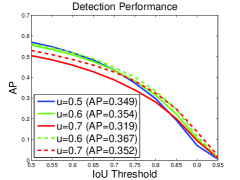
(a)

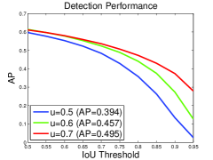
(b)

Figure 7: (a) detection performance of individually trained detectors, with their own proposals (solid curves) or Cascade R-CNN stage proposals (dashed curves). (b) results of adding ground truth to the proposal set.

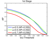
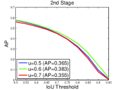
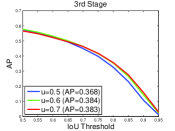
Figure 8: Detection performance of all Cascade R-CNN detectors at all cascade stages.

6.3 Comparison with Iterative BBox and Integral Loss

In this section, we compare the Cascade R-CNN to the iterative BBox and integral loss detectors. Iterative BBox was implemented by applying the detection head of FPN+ baseline iteratively at inference, three times. The integral loss detector was implemented with three classification heads, using $U=\{0.5,0.6,0.7\}$.

Localization: The localization performances of cascade regression and iterative BBox are compared in Fig. 9 (a). The use of a single regressor degrades localization for hypotheses of high IoU. This effect accumulates when the regressor is applied iteratively, as in iterative BBox, and performance actually drops with iteration number. Note the very poor performance of iterative BBox after 3 iterations. On the contrary, the cascade regressor has better performance at later stages, outperforming iterative BBox at almost all IoU levels. Note that, although cascade regression can slightly degrade high input IoUs, e.g. IoU$>$0.9, this decrease is negligible because, as shown in Fig. 4, the number of hypotheses with such high IoUs is extremely small.

Integral Loss: Figure 9 (b) summarizes the detection performances of all classifiers of the integral loss detector, sharing a single regressor. The classifier of $u=0.6$ is the best at all IoU levels, with $u=0.7$ producing the worst results. The ensemble of all classifiers shows no visible gain.

Table I shows that both iterative BBox and integral loss marginally improve on the baseline detector, and are not effective for high quality detection. On the other hand, the Cascade R-CNN achieves the best performance at all IoU levels. As expected, the gains are mild for low IoUs, e.g. 0.8 for AP₅₀, but significant for the higher ones, e.g. 6.1 for AP₈₀ and 8.7 for AP₉₀. Note that high quality object detection was rarely explored before this work. These experiments show that 1) it has more room for improvement than low quality detection, which focuses on AP₅₀, and 2) the overall AP can be significantly improved if it is effectively addressed.

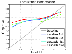
(a)

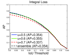
(b)

Figure 9: (a) localization performance of iterative BBox and Cascade R-CNN regressors. (b) detection performance of the individual classifiers of the integral loss detector.

	AP	AP50	AP60	AP70	AP80	AP90
FPN+ baseline	34.9	57.0	51.9	43.6	29.7	7.1
Iterative BBox	35.4	57.2	52.1	44.2	30.4	8.1
Integral Loss	35.4	57.3	52.5	44.4	29.9	6.9
Cascade R-CNN	38.9	57.8	53.4	46.9	35.8	15.8

TABLE I: Comparison of the Cascade R-CNN with iterative BBox and integral loss detectors.

6.4 Ablation Experiments

A few ablation experiments were run to enable a better understanding of the Cascade R-CNN.

Stage-wise Comparison: Table II summarizes stagewise performance. Note that the first stage already outperforms the baseline detector, due to the benefits of multi-stage multi-task learning. Since deeper cascade stages prefer higher quality localization, they encourage the learning of features conducive to it. This benefits the earlier cascade stages, due to the feature sharing by the backbone network. The second stage improves performance substantially, and the third is equivalent to the second. This differs from the integral loss detector, where the higher IoU classifier is relatively weak. While the former (later) stage is better at low (high) IoU metrics, the ensemble of all classifiers is the best overall.

IoU Thresholds: A Cascade R-CNN was trained using IoU threshold $u=0.5$ for all heads. In this case, the stages differ only in the hypotheses at their input. Each stage is trained with the corresponding hypotheses, i.e. accounting for the distribution changes of Fig. 5. The first row of Table III shows that this cascade improves on the baseline detector. This supports the claim that stages should be optimized for the corresponding sample distributions. The second row shows performance that improves further when the threshold $u$ increases across stages. As discussed in Section 4.3, the detector becomes more selective against close false positives and specialized to the more precise hypotheses.

test stage	AP	AP50	AP60	AP70	AP80	AP90
1	35.5	57.2	52.4	44.1	30.5	8.1
2	38.3	57.9	53.4	46.4	35.2	14.2
3	38.3	56.6	52.2	46.3	35.7	15.9
$\overline{1\sim{2}}$	38.5	58.2	53.8	46.7	35.0	14.0
$\overline{1\sim{3}}$	38.9	57.8	53.4	46.9	35.8	15.8
FPN+ baseline	34.9	57.0	51.9	43.6	29.7	7.1

TABLE II: Stagewise performance of the Cascade R-CNN. $\overline{1\sim{3}}$ indicates an ensemble result, obtained by averaging the three classifier probabilities for 3rd stage proposals.

IoU$\uparrow$	update	stage	AP	AP50	AP60	AP70	AP80	AP90
	statistics	loss
		decay	36.8	57.8	52.9	45.4	32.0	10.7
✓		decay	38.5	58.4	54.1	47.1	35.0	13.1
	✓	decay	37.5	57.8	53.1	45.5	33.3	13.1
✓	✓	decay	38.9	57.8	53.4	46.9	35.8	15.8
✓	✓	avg	38.9	57.5	53.4	46.9	35.8	16.2

TABLE III: Ablation experiments. “IoU$\uparrow$” indicates increasing IoU thresholds, “update statistics” updating regression statistics, and “stage loss” weighting of stage losses.

Regression Statistics: In Section 3.1.1, we saw that the distance vector $\Delta$ is normalized by the regression statistics (mean and variance), as in (5). In the Cascade R-CNN, these statistics are updated stage by stage, as illustrated in Fig. 5. Updating the statistics of (5) in deeper stages helps the effective multi-task learning of classification and regression. Empirically, the learning is not very sensitive to the exact values of these statistics. For simplicity, we set $\mu=0$ for all stages, $\Sigma=(\sigma_{x},\sigma_{y},\sigma_{w},\sigma_{h})=(0.1,0.1,0.2,0.2)$ for the first stage, $\Sigma/2$ for the second, and $\Sigma/3$ for the third, in all of our experiments. The third and fourth row of Table III show that this is beneficial, when compared to using the statistics of the first stage in all stages (the first and second row).

Stage Losses: The Cascade R-CNN has multiple detection heads, each with its own loss. We have explored two schemes to combine these losses: decay and avg. In avg, the loss of stage $t$ receives a weight $w_{t}=1/T$, where $T$ is the number of stages. In decay, the weight is $w_{t}=1/2^{t-1}$. For both schemes, the learning rate of the head parameters of stage $t$ is rescaled by $1/w_{t}$, to ensure that these are sufficiently trained. No rescaling is needed for the backbone network parameters, since they receive gradients from all stages. Table III shows that 1) avg has somewhat better performance for high quality metrics, but worse for low quality ones, and 2) the two methods have similar overall AP. The decay scheme is used in the remainder of the paper.

Number of Stages: Table IV summarizes the impact of the number of stages in the Cascade R-CNN performance. Adding a second stage significantly improves the baseline detector. Three detection stages still produce non-trivial improvement, but the addition of a $4^{th}$ stage ($u=0.75$) has a slight performance decrease. Note, however, that while the overall AP degrades, the four-stage cascade has the best performance at high IoU levels. The three-stage cascade achieves the best trade-off between cost and AP performance, and is used in the remaining experiments.

# stages	test stage	AP	AP50	AP60	AP70	AP80	AP90
1	1	34.9	57.0	51.9	43.6	29.7	7.1
2	$\overline{1\sim{2}}$	38.2	58.0	53.6	46.7	34.6	13.6
3	$\overline{1\sim{3}}$	38.9	57.8	53.4	46.9	35.8	15.8
4	$\overline{1\sim{3}}$	38.9	57.4	53.2	46.8	36.0	16.0
4	$\overline{1\sim{4}}$	38.6	57.2	52.8	46.2	35.5	16.3

TABLE IV: The impact of the number of stages in Cascade R-CNN.

	backbone	AP	AP50	AP75	APS	APM	APL
YOLOv2 [46]	DarkNet-19	21.6	44.0	19.2	5.0	22.4	35.5
SSD513 [40]∗	ResNet-101	31.2	50.4	33.3	10.2	34.5	49.8
RetinaNet [38]∗	ResNet-101	39.1	59.1	42.3	21.8	42.7	50.2
CornerNet [33]∗⋆	Hourglass-104	42.1	57.8	45.3	20.8	44.8	56.7
Faster R-CNN+++ [27]∗⋆	ResNet-101	34.9	55.7	37.4	15.6	38.7	50.9
Faster R-CNN w FPN [37]	ResNet-101	36.2	59.1	39.0	18.2	39.0	48.2
Faster R-CNN w FPN+ (ours)	ResNet-101	38.8	61.1	41.9	21.3	41.8	49.8
G-RMI [29]∗⋆	Inception-ResNet-v2	41.6	62.3	45.6	24.0	43.9	55.2
Deformable R-FCN [9]∗⋆	Aligned-Inception-ResNet	37.5	58.0	40.8	19.4	40.1	52.5
Mask R-CNN [25]	ResNet-101	38.2	60.3	41.7	20.1	41.1	50.2
RelationNet [28]	ResNet-101	39.0	58.6	42.9	-	-	-
DetNet [35]	DetNet-59	40.3	62.1	43.8	23.6	42.6	50.0
SNIP [52]∗⋆	DPN-98	45.7	67.3	51.1	29.3	48.8	57.1
AttractioNet [18]⋆	VGG16+Wide ResNet	35.7	53.4	39.3	15.6	38.0	52.7
Cascade R-CNN	ResNet-101	42.8	62.1	46.3	23.7	45.5	55.2
Cascade R-CNN∗⋆	ResNeXt-152	50.9	69.0	55.8	33.4	53.5	63.3

TABLE V: Performance of state-of-the-art single-model detectors on COCO test-dev. Entries denoted by ^∗ and ^⋆ use enhancements at training and inference, respectively.

	backbone	cascade	train	test	model	val (5k)						test-dev (20k)
			speed	speed	size	AP	AP50	AP75	APS	APM	APL	AP	AP50	AP75	APS	APM	APL
Faster R-CNN	VGG	✗	0.12s	0.075s	278M	23.6	43.9	23.0	8.0	26.2	35.5	23.5	43.9	22.6	8.1	25.1	34.7
		✓	0.14s	0.115s	704M	27.0	44.2	27.7	8.6	29.1	42.2	26.9	44.3	27.8	8.3	28.2	41.1
R-FCN	ResNet-50	✗	0.19s	0.07s	133M	27.0	48.7	26.9	9.8	30.9	40.3	27.1	49.0	26.9	10.4	29.7	39.2
		✓	0.24s	0.075s	184M	31.1	49.8	32.8	10.4	34.4	48.5	30.9	49.9	32.6	10.5	33.1	46.9
R-FCN	ResNet-101	✗	0.23s	0.075s	206M	30.3	52.2	30.8	12.0	34.7	44.3	30.5	52.9	31.2	12.0	33.9	43.8
		✓	0.29s	0.083s	256M	33.3	52.0	35.2	11.8	37.2	51.1	33.3	52.6	35.2	12.1	36.2	49.3
FPN+	ResNet-50	✗	0.30s	0.095s	165M	36.5	58.6	39.2	20.8	40.0	47.8	36.5	59.0	39.2	20.3	38.8	46.4
		✓	0.33s	0.115s	272M	40.3	59.4	43.7	22.9	43.7	54.1	40.6	59.9	44.0	22.6	42.7	52.1
FPN+	ResNet-101	✗	0.38s	0.115s	238M	38.5	60.6	41.7	22.1	41.9	51.1	38.8	61.1	41.9	21.3	41.8	49.8
		✓	0.41s	0.14s	345M	42.7	61.6	46.6	23.8	46.2	57.4	42.8	62.1	46.3	23.7	45.5	55.2

TABLE VI: Performance of Cascade R-CNN implementations with multiple detectors. All speeds are reported per image on a single Titan Xp GPU.

6.5 Comparison with the state-of-the-art

An implementation of the Cascade R-CNN, based on the FPN+ detector and the ResNet-101 backbone, is compared to state-of-the-art single-model detectors in Table V. The settings are those of Section 6.1.3, but training used 280k iterations, with learning rate decreased at 160k and 240k iterations. The number of RoIs was also increased to 512. The top of the table reports to one-stage detectors, the middle to two-stage, and the bottom to multi-stage (3-stages+RPN for the Cascade R-CNN). Note that all the compared state-of-the-art detectors are trained with $u=0.5$.

An initial observation is that our FPN+ implementation is better than the original FPN [37], providing a very strong baseline. Nevertheless, the extension from FPN+ to Cascade R-CNN improved performance by $\sim$4 points. In fact, the vanilla Cascade R-CNN, without any bells and whistles, outperformed almost all single-model detectors under all evaluation metrics. This includes the COCO challenge 2016 winner G-RMI [29], the recent Deformable R-FCN [9], RetinaNet [38], Mask R-CNN [25], RelationNet[28], DetNet[35], CornerNet [33], etc. Note some of these methods leverage several training or inference enhancements, e.g. multi-scale, soft NMS [1], etc, making the comparison very unfair. Finally, compared to the previously best multi-stage detector on COCO, AttractioNet [18], the vanilla Cascade R-CNN has a gain of 7.1 points.

The only detector that outperforms the Cascade R-CNN in Table V is SNIP [52], which uses multi-scale training and inference, a larger input size, a stronger backbone, Soft NMS, and some other enhancements. For a more fair comparison, we implemented the Cascade R-CNN with multi-scale training/inference, a stronger backbone (ResNeXt-152 [57]), mask supervision, etc. This enhanced Cascade R-CNN surpassed SNIP by 5.2 points. It also outperforms the single-model MegDet detector (50.6 mAP), which won the COCO challenge in 2017 and uses many other enhancements [45]. The Cascade R-CNN is conceptually straightforward, simple to implement, and can be combined, in a plug and play manner, with many detector architectures.

6.6 Generalization Capacity

To more thoroughly test this claim, a three-stage Cascade R-CNN was implemented with three baseline detectors: Faster R-CNN, R-FCN, and FPN+. All settings are as discussed above, with the variations discussed in Section 6.5 for the FPN+ detector. Table VI presents a comparison of the AP performance of the three detectors.

Detection Performance: Again, our implementations are better than the original detectors [47, 8, 37]. Still, the Cascade R-CNN improves on all baselines by 2$\sim$4 points, independently of their strength. Similar gains are observed for val and test-dev. These results show that the Cascade R-CNN is widely applicable across detector architectures.

Parameters and Timing: The number of Cascade R-CNN parameters increases with the number of stages. The increase is linear and proportional to the parameter cardinality of the baseline detector head. However, because the head has much less computation than the backbone network, the Cascade R-CNN has small computational overhead, at both training and testing. This is shown in Table VI.

Codebase and Backbone: The Cascade R-CNN of FPN was also reimplemented on the Detectron codebase [20] with various backbone networks. Table VII summarizes these experiments, showing very consistent improvements (3$\sim$4 points) across backbones. The Cascade R-CNN has also been independently reproduced by other research groups, on PyTorch and TensorFlow. These again show that the Cascade R-CNN can provide reliable gains across detector architectures, backbones, codebases, and implementations.

backbone	cascade	AP	AP50	AP75	APS	APM	APL
Fast ResNet-50	✗	36.4	58.4	39.3	20.3	39.8	48.1
	✓	40.5	58.7	43.9	21.5	43.6	54.9
ResNet-50	✗	36.7	58.4	39.6	21.1	39.8	48.1
	✓	40.9	59.0	44.6	22.5	43.6	55.3
ResNet-101	✗	39.4	61.2	43.4	22.6	42.9	51.4
	✓	42.8	61.4	46.8	24.1	45.8	57.4
ResNeXt-101	✗	41.3	63.7	44.7	25.5	45.3	52.9
	✓	44.7	63.7	48.8	26.3	48.4	58.6
ResNet-50-GN	✗	38.4	59.9	41.7	22.2	41.2	50.0
	✓	42.2	60.6	45.8	24.7	45.2	55.7
ResNet-101-GN	✗	39.9	61.3	43.3	23.6	42.8	52.3
	✓	43.8	62.2	47.6	26.2	47.2	57.7

TABLE VII: Performance of various implementations of the Cascade R-CNN with the FPN detector on Detectron, using the 1x schedule.

Fast R-CNN: As shown in Fig. 3 (b), the Cascade R-CNN is not limited to the standard Faster R-CNN architecture. To test this, we trained the Cascade R-CNN in the way of the Fast R-CNN, using pre-collected proposals. The results of Table VII show that the gains of the Cascade R-CNN hold for frameworks other than the Faster R-CNN.

Group Normalization: Group normalization (GN) [56] is a recent normalization technique, published after the Cascade R-CNN. It addresses the problem that batch normalization (BN) [30] must be frozen for object detector training, due to the inaccurate statistics that can be derived from small batch sizes [45]. GN, an alternative to BN that is independent of batch size, has comparable performance to large-batch synchronized BN. Table VII shows that the Cascade R-CNN with GN has similar gains to those obersved for the other architectures. This suggests that the Cascade R-CNN will continue to be useful even as architectural enhancements continue to emerge in the literature.

stage	AP100	AP${}^{100}_{s}$	AP${}^{100}_{m}$	AP${}^{100}_{l}$	AP1k	AP${}^{1k}_{s}$	AP${}^{1k}_{m}$	AP${}^{1k}_{l}$
FPN	47.8	32.2	54.9	65.2	59.1	48.0	66.3	68.4
1	46.8	31.0	53.8	64.8	58.7	47.6	65.9	68.2
2	55.3	35.1	61.1	82.5	70.7	55.2	77.7	88.1
3	56.5	36.1	62.4	84.1	71.4	55.5	78.1	89.8

TABLE VIII: Proposal recall of Cascade R-CNN stages.

6.7 Proposal Evaluation

Table VIII summarizes the proposal recall performance of a Cascade R-CNN implemented with the FPN detector and ResNet-50 backbone. The first Cascade R-CNN stage has proposal recall close to that of the FPN baseline. The addition of a bounding box regression stage improves recall significantly, e.g. from 59.1 to 70.7 for AP^1k and close to 20 points for AP${}^{1k}_{l}$. This shows that the additional bounding box regression is very effective at improving proposal recall performance. The addition of a third stage has a smaller but non-negligible gain. This high proposal recall performance secures the later high-quality object detection task.

6.8 Instance Segmentation by Cascade Mask R-CNN

Table IX summarizes the instance segmentation performance of the Cascade Mask R-CNN strategies of Fig. 6. These experiments, use the Mask R-CNN, implemented on Detectron with 1x schedule as baseline. All three strategies improve on baseline performance, although with smaller gains than object detection (see Table II), especially at high quality. For example, the AP₉₀ improvement of 8.7 points for object detection falls to 1.8 points, showing that plenty of room is left for improving high quality instance segmentation. Comparing strategies, (c) outperforms (b). This is because (b) trains the mask head in the first stage but tests after the last stage, leading to a mask prediction mismatch. This mismatch is reduced by (c). The addition of a mask branch to each stage by strategy (d) does not have noticeable benefits over (c), but requires much more computation and memory. Strategy (b) has the best trade-off between cost and AP performance, and is used in the remainder of the paper.

To evaluate the instance segmentation robustness of the Cascade Mask R-CNN, several backbone networks are compared in Table X. Since this architecture can detect objects, detection results are also shown. Note that the additional mask supervision makes these better than those of Table VII. The gains of the Cascade Mask R-CNN are very consistent for all backbone networks. Even when the strongest model, ResNeXt-152 [57], is used with training data augmentation and 1.44x schedule, the Cascade Mask R-CNN has a gain of 2.9 points for detection and 1.0 point for instance segmentation. Adding inference enhancements, the gains are still 2.1 points for detection and 0.8 points for instance segmentation. This robustness explains why the Cascade R-CNN was widely used in the COCO challenge 2018, where the task is instance segmentation, not object detection.

	AP	AP50	AP60	AP70	AP80	AP90
Mask R-CNN baseline	33.9	55.5	49.8	41.4	28.6	8.3
strategy of Fig. 6 (b)	35.0	56.3	50.8	43.0	30.0	9.3
strategy of Fig. 6 (c)	35.4	56.4	50.9	43.2	31.0	10.1
strategy of Fig. 6 (d)	35.5	56.5	51.2	43.4	30.8	10.0

TABLE IX: The instance segmentation comparison among three strategies of the Cascade Mask R-CNN.

backbone	cascade	Object Detection						Instance Segmentation
		AP	AP50	AP75	APS	APM	APL	AP	AP50	AP75	APS	APM	APL
ResNet-50	✗	37.7	59.2	40.9	21.4	40.8	49.8	33.9	55.8	35.8	14.9	36.3	50.9
	✓	41.3	59.4	45.3	23.2	43.8	55.8	35.4	56.4	37.7	15.9	37.7	53.6
ResNet-101	✗	40.0	61.8	43.7	22.5	43.4	52.7	35.9	58.3	38.0	15.9	38.9	53.2
	✓	43.3	61.7	47.2	24.2	46.3	58.2	37.1	58.6	39.8	16.7	39.7	55.7
ResNet-50-GN	✗	39.2	60.5	42.9	22.9	42.2	50.6	34.9	57.1	36.9	16.0	37.7	51.2
	✓	42.9	60.7	46.6	25.1	45.9	56.7	36.6	57.7	39.2	16.8	39.3	54.5
ResNet-101-GN	✗	41.1	62.1	45.1	23.6	44.3	53.1	36.3	58.9	38.5	16.2	39.4	53.6
	✓	44.8	62.8	48.8	26.4	48.0	58.7	38.0	59.8	40.8	18.1	40.7	56.0
ResNeXt-101	✗	42.1	64.1	45.9	25.6	45.9	54.4	37.3	60.3	39.5	17.8	40.3	55.5
	✓	45.8	64.1	50.3	27.2	49.5	60.1	38.6	60.6	41.5	18.5	41.3	57.2
ResNeXt-152∗	✗	45.2	66.9	49.7	28.5	49.4	56.8	39.7	63.5	42.4	19.8	42.9	57.3
	✓	48.1	66.7	52.6	29.3	52.2	62.1	40.7	63.7	43.8	19.9	44.0	59.1
ResNeXt-152∗⋆	✗	48.1	68.3	52.9	32.6	51.8	61.3	41.5	65.1	44.7	22.0	44.8	59.8
	✓	50.2	68.2	55.0	33.1	53.9	64.2	42.3	65.4	45.8	21.9	45.7	60.9

TABLE X: Performance of the Cascade Mask R-CNN on multiple backbone networks on COCO 2017 val. ^∗ and ^⋆ denotes enhancement techniques at training and inference, respectively, as in [20].

6.9 Results on PASCAL VOC

The Cascade R-CNN was further tested on the PASCAL VOC dataset [13]. Following [47, 40], the models were trained on VOC2007 and VOC2012 trainval (16,551 images) and tested on VOC2007 test (4,952 images). Two detector architectures were evaluated: Faster R-CNN (with AlexNet and VGG-Net backbones) and R-FCN (with ResNet-50 and ResNet-101). Training details were as discussed in Section 6.1.3, and both AlexNet and VGG-Net were pruned. More specifically, Faster R-CNN (R-FCN) training started with a learning rate of 0.001 (0.002), which was reduced by a factor of 10 at 30k (60k) and stopped at 45k (90k) iterations. Since the standard VOC evaluation metric (AP at IoU of 0.5) is fairly saturated, and the focus of this work is high quality detection, the COCO metrics were used for evaluation. Table XI summarizes the performance of all detectors, showing that the Cascade R-CNN significantly improves the overall AP in all cases. These results are further evidence for the robustness of the Cascade R-CNN.

6.10 Additional Results on other Datasets

Beyond generic object detection datasets, the Cascade R-CNN was tested on some specific object detection tasks, including KITTI [16], CityPerson [64] and WiderFace [61]. The MS-CNN [2], a detector of strong performance on these tasks, was used as baseline for all of them.

KITTI: One of the most popular datasets for autonomous driving, KITTI contains 7,481 training/validation images, and 7,518 for testing with held annotations. The 2D object detection task contains three categories: car, pedestrian, and cyclist. Evaluation is based on the VOC AP at IoU of 0.7, 0.5, and 0.5 for the three categories, respectively. Since the focus of this work is high quality detection, the Cascade R-CNN was only tested on the car category. As shown in Table XII, it improved the baseline by 0.87 points for the Moderate, and 1.9 points for the Hard regime, on the test set. These improvements are nontrivial, given that MS-CNN is a strong detector and the KITTI car detection task is fairly saturated.

CityPersons: CityPersons is a recently published pedestrian detection dataset, collected across multiple European cities. It contains 2,975 training and 500 validation images, and 1,575 images for testing with held annotations. Evaluation is based on miss-rate (MR) at IoU=0.5. We also report results for MR at IoU=0.75, which is more commensurate with high quality detection. This is consistent with a recent trend to adopt the stricter COCO metric for pedestrian and face detection, see e.g. the Wider Challenge 2018. Table XIII compares the validation set performance of the Cascade R-CNN with that of the baseline MS-CNN (performances on validation and test sets are usually equivalent on this dataset). The Cascade R-CNN has large performance gains, especially for the stricter evaluation metric. For example, it improves the baseline performance by $\sim$10 points on the Reasonable set at MR₇₅.

	backbone	cascade	AP	AP50	AP75
Faster R-CNN	AlexNet	✗	29.4	63.2	23.7
		✓	38.9	66.5	40.5
Faster R-CNN	VGG	✗	42.9	76.4	44.1
		✓	51.2	79.1	56.3
R-FCN	RetNet-50	✗	44.8	77.5	46.8
		✓	51.8	78.5	57.1
R-FCN	ResNet-101	✗	49.4	79.8	53.2
		✓	54.2	79.6	59.2

TABLE XI: Detection results on PASCAL VOC 2007 test.

	cascade	Easy	Moderate	Hard
AP70	✗	90.22	89.08	76.50
	✓	90.68	89.95	78.40

TABLE XII: MS-CNN detection results for the car class on KITTI test set.

	cascade	Reasonable	Small	Heavy	All
MR50	✗	13.07	40.42	53.55	38.74
	✓	11.96	38.37	49.41	36.83
MR75	✗	38.23	59.84	85.06	65.56
	✓	28.45	56.24	81.86	58.24

TABLE XIII: MS-CNN detection results on CityPersons validation set.

WiderFace: One of the most challenging face detection datasets, mainly due to its diversity in scale, pose and occlusion, WiderFace contains 32,203 images with 393,703 annotated faces, of which 12,880 are used for training, 3,226 for validation, and the remainder for testing with held annotations. Evaluation is based on the VOC AP at IoU=0.5 on three subsets, easy, medium and hard, of different detection difficulty. Again, we have used AP at IoU=0.5 and IoU=0.75 and evaluation on the validation set. Table XIV shows that, while the Cascade R-CNN is close to the baseline MS-CNN for AP₅₀, it significantly boosts its performance for AP₇₅. The gain is smaller on the hard than on the easy and medium, because the former contains mainly very small and heavily occluded faces, for which high quality detection is difficult. This observation mirrors the COCO experiments of Table VI, where improvements in AP_S are smaller than for AP_L.

	cascade	Easy	Medium	Hard
AP50	✗	91.1	90.6	81.0
	✓	91.3	90.3	81.1
AP75	✗	59.7	61.3	40.7
	✓	68.7	66.3	42.8

TABLE XIV: MS-CNN Detection results on WiderFace validation set.

7 Conclusion

In this work, we have proposed a multi-stage object detection framework, the Cascade R-CNN, for high quality object detection, a rarely explored problem in the detection literature. This architecture was shown to overcome the high quality detection challenges of overfitting during training and quality mismatch during inference. This is achieved by training stages sequentially, using the output of one to train the next, and the same cascade is applied at inference. The Cascade R-CNN was shown to achieve very consistent performance gains on multiple challenging datasets, including COCO, PASCAL VOC, KITTI, CityPersons, and WiderFace, for both generic and specific object detection. These gains were also observed for many object detectors, backbone networks, and techniques for detection and instance segmentation. We thus believe that the Cascade R-CNN can be useful for many future object detection and instance segmentation research efforts.

Acknowledgment: This work was funded by NSF Awards IIS-1546305 and IIS-1637941, and a GPU donation from NVIDIA. We would also like to thank Kaiming He for valuable discussions.

References

- [1] N. Bodla, B. Singh, R. Chellappa, and L. S. Davis. Soft-nms - improving object detection with one line of code. In ICCV, pages 5562–5570, 2017.
- [2] Z. Cai, Q. Fan, R. S. Feris, and N. Vasconcelos. A unified multi-scale deep convolutional neural network for fast object detection. In ECCV, pages 354–370, 2016.
- [3] Z. Cai and N. Vasconcelos. Cascade R-CNN: Delving into high quality object detection. In CVPR, 2018.
- [4] X. Cao, Y. Wei, F. Wen, and J. Sun. Face alignment by explicit shape regression. In CVPR, pages 2887–2894, 2012.
- [5] K. Chen, J. Pang, J. Wang, Y. Xiong, X. Li, S. Sun, W. Feng, Z. Liu, J. Shi, W. Ouyang, C. C. Loy, and D. Lin. Hybrid task cascade for instance segmentation. CoRR, abs/1901.07518, 2019.
- [6] C. Cortes and V. Vapnik. Support-vector networks. Machine Learning, 20(3):273–297, 1995.
- [7] J. Dai, K. He, and J. Sun. Instance-aware semantic segmentation via multi-task network cascades. In CVPR, pages 3150–3158, 2016.
- [8] J. Dai, Y. Li, K. He, and J. Sun. R-FCN: object detection via region-based fully convolutional networks. In NIPS, pages 379–387, 2016.
- [9] J. Dai, H. Qi, Y. Xiong, Y. Li, G. Zhang, H. Hu, and Y. Wei. Deformable convolutional networks. In ICCV, 2017.
- [10] P. Dollár, P. Welinder, and P. Perona. Cascaded pose regression. In CVPR, pages 1078–1085, 2010.
- [11] P. Dollár, C. Wojek, B. Schiele, and P. Perona. Pedestrian detection: An evaluation of the state of the art. IEEE Trans. Pattern Anal. Mach. Intell., 34(4):743–761, 2012.
- [12] C. Elkan. The foundations of cost-sensitive learning. In IJCAI, pages 973–978, 2001.
- [13] M. Everingham, L. J. V. Gool, C. K. I. Williams, J. M. Winn, and A. Zisserman. The pascal visual object classes (VOC) challenge. International Journal of Computer Vision, 88(2):303–338, 2010.
- [14] P. F. Felzenszwalb, R. B. Girshick, D. A. McAllester, and D. Ramanan. Object detection with discriminatively trained part-based models. IEEE Trans. Pattern Anal. Mach. Intell., 32(9):1627–1645, 2010.
- [15] Y. Freund and R. E. Schapire. A decision-theoretic generalization of on-line learning and an application to boosting. In EuroCOLT, pages 23–37, 1995.
- [16] A. Geiger, P. Lenz, and R. Urtasun. Are we ready for autonomous driving? the KITTI vision benchmark suite. In CVPR, pages 3354–3361, 2012.
- [17] S. Gidaris and N. Komodakis. Object detection via a multi-region and semantic segmentation-aware CNN model. In ICCV, pages 1134–1142, 2015.
- [18] S. Gidaris and N. Komodakis. Attend refine repeat: Active box proposal generation via in-out localization. In BMVC, 2016.
- [19] S. Gidaris and N. Komodakis. Locnet: Improving localization accuracy for object detection. In CVPR, pages 789–798, 2016.
- [20] R. Girshick, I. Radosavovic, G. Gkioxari, P. Dollár, and K. He. Detectron. https://github.com/facebookresearch/detectron, 2018.
- [21] R. B. Girshick. Fast R-CNN. In ICCV, pages 1440–1448, 2015.
- [22] R. B. Girshick, J. Donahue, T. Darrell, and J. Malik. Rich feature hierarchies for accurate object detection and semantic segmentation. In CVPR, pages 580–587, 2014.
- [23] S. Han, J. Pool, J. Tran, and W. J. Dally. Learning both weights and connections for efficient neural network. In NIPS, pages 1135–1143, 2015.
- [24] K. He, R. Girshick, and P. Dollár. Rethinking imagenet pre-training. arXiv preprint arXiv:1811.08883, 2018.
- [25] K. He, G. Gkioxari, P. Dollár, and R. Girshick. Mask r-cnn. In ICCV, 2017.
- [26] K. He, X. Zhang, S. Ren, and J. Sun. Spatial pyramid pooling in deep convolutional networks for visual recognition. In ECCV, pages 346–361, 2014.
- [27] K. He, X. Zhang, S. Ren, and J. Sun. Deep residual learning for image recognition. In CVPR, pages 770–778, 2016.
- [28] H. Hu, J. Gu, Z. Zhang, J. Dai, and Y. Wei. Relation networks for object detection. In IEEE CVPR, volume 2, 2018.
- [29] J. Huang, V. Rathod, C. Sun, M. Zhu, A. Korattikara, A. Fathi, I. Fischer, Z. Wojna, Y. Song, S. Guadarrama, and K. Murphy. Speed/accuracy trade-offs for modern convolutional object detectors. CoRR, abs/1611.10012, 2016.
- [30] S. Ioffe and C. Szegedy. Batch normalization: Accelerating deep network training by reducing internal covariate shift. In ICML, pages 448–456, 2015.
- [31] Y. Jia, E. Shelhamer, J. Donahue, S. Karayev, J. Long, R. B. Girshick, S. Guadarrama, and T. Darrell. Caffe: Convolutional architecture for fast feature embedding. In MM, pages 675–678, 2014.
- [32] B. Jiang, R. Luo, J. Mao, T. Xiao, and Y. Jiang. Acquisition of localization confidence for accurate object detection. In ECCV, pages 816–832, 2018.
- [33] H. Law and J. Deng. Cornernet: Detecting objects as paired keypoints. In ECCV, pages 765–781, 2018.
- [34] H. Li, Z. Lin, X. Shen, J. Brandt, and G. Hua. A convolutional neural network cascade for face detection. In CVPR, pages 5325–5334, 2015.
- [35] Z. Li, C. Peng, G. Yu, X. Zhang, Y. Deng, and J. Sun. Detnet: Design backbone for object detection. In ECCV, pages 339–354, 2018.
- [36] T. Lin, M. Maire, S. J. Belongie, J. Hays, P. Perona, D. Ramanan, P. Dollár, and C. L. Zitnick. Microsoft COCO: common objects in context. In ECCV, pages 740–755, 2014.
- [37] T.-Y. Lin, P. Dollár, R. Girshick, K. He, B. Hariharan, and S. Belongie. Feature pyramid networks for object detection. In CVPR, 2017.
- [38] T.-Y. Lin, P. Goyal, R. Girshick, K. He, and P. Dollár. Focal loss for dense object detection. In ICCV, 2017.
- [39] S. Liu, L. Qi, H. Qin, J. Shi, and J. Jia. Path aggregation network for instance segmentation. In IEEE CVPR, pages 8759–8768, 2018.
- [40] W. Liu, D. Anguelov, D. Erhan, C. Szegedy, S. E. Reed, C. Fu, and A. C. Berg. SSD: single shot multibox detector. In ECCV, pages 21–37, 2016.
- [41] W. Liu, S. Liao, W. Hu, X. Liang, and X. Chen. Learning efficient single-stage pedestrian detectors by asymptotic localization fitting. In ECCV, pages 643–659, 2018.
- [42] H. Masnadi-Shirazi and N. Vasconcelos. Cost-sensitive boosting. IEEE Trans. Pattern Anal. Mach. Intell., 33(2):294–309, 2011.
- [43] M. Najibi, M. Rastegari, and L. S. Davis. G-CNN: an iterative grid based object detector. In CVPR, pages 2369–2377, 2016.
- [44] W. Ouyang, K. Wang, X. Zhu, and X. Wang. Learning chained deep features and classifiers for cascade in object detection. CoRR, abs/1702.07054, 2017.
- [45] C. Peng, T. Xiao, Z. Li, Y. Jiang, X. Zhang, K. Jia, G. Yu, and J. Sun. Megdet: A large mini-batch object detector. In IEEE CVPR, pages 6181–6189, 2018.
- [46] J. Redmon, S. K. Divvala, R. B. Girshick, and A. Farhadi. You only look once: Unified, real-time object detection. In CVPR, pages 779–788, 2016.
- [47] S. Ren, K. He, R. B. Girshick, and J. Sun. Faster R-CNN: towards real-time object detection with region proposal networks. In NIPS, pages 91–99, 2015.
- [48] O. Russakovsky, J. Deng, H. Su, J. Krause, S. Satheesh, S. Ma, Z. Huang, A. Karpathy, A. Khosla, M. S. Bernstein, A. C. Berg, and F. Li. Imagenet large scale visual recognition challenge. International Journal of Computer Vision, 115(3):211–252, 2015.
- [49] M. J. Saberian and N. Vasconcelos. Learning optimal embedded cascades. IEEE Trans. Pattern Anal. Mach. Intell., 34(10):2005–2018, 2012.
- [50] A. Shrivastava, A. Gupta, and R. B. Girshick. Training region-based object detectors with online hard example mining. In CVPR, pages 761–769, 2016.
- [51] K. Simonyan and A. Zisserman. Very deep convolutional networks for large-scale image recognition. CoRR, abs/1409.1556, 2014.
- [52] B. Singh and L. S. Davis. An analysis of scale invariance in object detection–snip. In IEEE CVPR, pages 3578–3587, 2018.
- [53] J. R. R. Uijlings, K. E. A. van de Sande, T. Gevers, and A. W. M. Smeulders. Selective search for object recognition. International Journal of Computer Vision, 104(2):154–171, 2013.
- [54] P. A. Viola and M. J. Jones. Robust real-time face detection. International Journal of Computer Vision, 57(2):137–154, 2004.
- [55] X. Wu, D. Zhang, J. Zhu, and S. C. H. Hoi. Single-shot bidirectional pyramid networks for high-quality object detection. CoRR, abs/1803.08208, 2018.
- [56] Y. Wu and K. He. Group normalization. In ECCV, pages 3–19, 2018.
- [57] S. Xie, R. B. Girshick, P. Dollár, Z. Tu, and K. He. Aggregated residual transformations for deep neural networks. In CVPR, pages 5987–5995, 2017.
- [58] X. Xiong and F. D. la Torre. Supervised descent method and its applications to face alignment. In CVPR, pages 532–539, 2013.
- [59] J. Yan, Z. Lei, D. Yi, and S. Li. Learn to combine multiple hypotheses for accurate face alignment. In ICCV Workshops, pages 392–396, 2013.
- [60] B. Yang, J. Yan, Z. Lei, and S. Z. Li. CRAFT objects from images. In CVPR, pages 6043–6051, 2016.
- [61] S. Yang, P. Luo, C. C. Loy, and X. Tang. WIDER FACE: A face detection benchmark. In CVPR, pages 5525–5533, 2016.
- [62] D. Yoo, S. Park, J. Lee, A. S. Paek, and I. Kweon. Attentionnet: Aggregating weak directions for accurate object detection. In ICCV, pages 2659–2667, 2015.
- [63] S. Zagoruyko, A. Lerer, T. Lin, P. O. Pinheiro, S. Gross, S. Chintala, and P. Dollár. A multipath network for object detection. In BMVC, 2016.
- [64] S. Zhang, R. Benenson, and B. Schiele. Citypersons: A diverse dataset for pedestrian detection. In CVPR, pages 4457–4465, 2017.
- [65] S. Zhang, L. Wen, X. Bian, Z. Lei, and S. Z. Li. Single-shot refinement neural network for object detection. In IEEE CVPR, 2018.