Generalization of Fourier’s law into viscous heat equations

Abstract

Heat conduction in dielectric crystals originates from the propagation of atomic vibrations, whose microscopic dynamics is well described by the linearized phonon Boltzmann transport equation. Recently, it was shown that thermal conductivity can be resolved exactly and in a closed form as a sum over relaxons, i.e. collective phonon excitations that are the eigenvectors of Boltzmann equation’s scattering matrix [Cepellotti and Marzari, Phys. Rev. X 6, 041013 (2016)]. Relaxons have a well-defined parity, and only odd relaxons contribute to the thermal conductivity. Here, we show that the complementary set of even relaxons determines another quantity — the thermal viscosity — that enters into the description of heat transport, and is especially relevant in the hydrodynamic regime, where dissipation of crystal momentum by Umklapp scattering phases out. We also show how the thermal conductivity and viscosity parametrize two novel viscous heat equations — two coupled equations for the temperature and drift-velocity fields — which represent the thermal counterpart of the Navier-Stokes equations of hydrodynamics in the linear, laminar regime. These viscous heat equations are derived from a coarse-graining of the linearized Boltzmann transport equation for phonons, and encompass both limits of Fourier’s law and of second sound, taking place, respectively, in the regimes of strong or weak momentum dissipation. Last, we introduce the Fourier deviation number as a descriptor that captures the deviations from Fourier’s law due to hydrodynamic effects. We showcase these findings in a test case of a complex-shaped device made of graphite, obtaining a remarkable agreement with the very recent experimental demonstration of hydrodynamic transport in this material. The present findings also suggest that hydrodynamic behavior can appear at room temperature in micrometer-sized diamond crystals. The present formulation rigorously generalizes Fourier’s heat equation, extending the reach of physical and computational models for heat conduction also to the hydrodynamic regime.

I Introduction

Thermal transport in insulating crystals takes place through the evolution and dynamics of the vibrations of atoms around their equilibrium positions. The first predictive theoretical framework to describe thermal transport was developed by Peierls in 1929 Peierls (1929, 1955); Ziman (1960), who envisioned a microscopic theory in terms of a Boltzmann transport equation (BTE) for the propagation of vibrational excitations (phonon wavepackets). In the 1960s significant progress took place in this field, propelled by newly discovered hydrodynamic phenomena in crystals, with striking signatures such as Poiseuille-like heat flow Mezhov-Deglin (1966) and second sound Ackerman et al. (1966). The former manifests itself with a heat flux that is akin to the flow of a fluid in a pipe (i.e. showing a parabolic-like profile with a maximum in the center and minimum at the boundaries, due to viscous effects); the latter instead results in heat propagation in the form of a coherent temperature wave, rather than a diffusing heat front. Second sound has been observed experimentally in a handful of solids; first, in solid helium Ackerman et al. (1966), followed by sodium fluoride Jackson et al. (1970); Pohl and Irniger (1976), bismuth Narayanamurti and Dynes (1972), sapphire Danil’Chenko et al. (1979), and strontium titanate Hehlen et al. (1995); Koh and Cahill (2007) – all at cryogenic conditions. Importantly, neither Poiseuille flow nor second sound can be described by the macroscopic Fourier’s equation, which is limited to a diffusive description of heat propagation.

These experimental observations have been accompanied by several pioneering efforts aimed at providing a quantitative description of heat hydrodynamics at the mesoscopic level, i.e. in terms of partial differential equations (PDEs) that are simpler than the microscopic integro-differential BTE (we use “mesoscopic model” to denote any description requiring more fields or PDEs than the Fourier’s PDE for the temperature field Bergamasco et al. (2018)). Sussmann and Thellung Sussmann and Thellung (1963), starting from the linearized BTE (LBTE) in the absence of momentum-dissipating (Umklapp) phonon-phonon scattering events, derived mesoscopic equations in terms of the temperature and of the phonon drift velocity, i.e. the thermal counterparts of pressure and fluid velocity in liquids. Further advances came from Gurzhi Gurzhi (1964, 1968) and Guyer & Krumhansl Guyer and Krumhansl (1966a, b) who, including the effect of weak crystal momentum dissipation, obtained equations for damped second sound and for Poiseuille heat flow. Among early works, we also mention the discussions of phonon hydrodynamics in the framework of many-body theory, as in Refs. Griffin (1965); Enz (1968). While correctly capturing the qualitative features of phonon hydrodynamics, all the theoretical investigations mentioned above assume simplified phonon dispersion relations (either power-law Gurzhi (1964, 1968) or linear isotropic Sussmann and Thellung (1963); Guyer and Krumhansl (1966a, b)), or neglect momentum dissipation Sussmann and Thellung (1963). A more rigorous and general formulation — albeit valid only in the hydrodynamic regime of weak Umklapp scattering — was introduced by Hardy, who extended the study of second sound Hardy (1970) and, together with Albers, of Poiseuille flow in terms of mesoscopic transport equations Hardy and Albers (1974).

The turn of the century brought renewed interest in the theory of heat conduction; computational and algorithmic advances now allow to solve exactly the LBTE — employing iterative Omini and Sparavigna (1995); Broido et al. (2007); Carrete et al. (2017), variational Fugallo et al. (2013), or exact diagonalization Chaput (2013); Cepellotti and Marzari (2016) methods — and thus investigate the accuracy of the LBTE and the models derived from it. In addition, nowadays it is possible to solve the LBTE without any fitting parameter, deriving all quantities from first-principles; this has been shown to describe accurately the thermal properties of bulk crystals Broido et al. (2007); Esfarjani et al. (2011); Luckyanova et al. (2012); Cahill et al. (2014); Cepellotti et al. (2015); Paulatto et al. (2013, 2015); Lindsay (2016); Cepellotti and Marzari (2017a); Omini and Sparavigna (1996); McGaughey et al. (2019), provided phonon branches remain well-separated Simoncelli, M. and Marzari, N. and Mauri, F. (2019).

Further applications of the LBTE, combined with state-of-the-art first-principles simulations, have also recently predicted the existence of hydrodynamic phenomena at non-cryogenic temperatures in low-dimensional or layered materials such as graphene Lee et al. (2015); Cepellotti et al. (2015); Cepellotti and Marzari (2017b), other 2D materials Cepellotti et al. (2015), carbon nanotubes Lee and Lindsay (2017) and graphite Ding et al. (2018). Fittingly, and remarkably, these theoretical suggestions have now been confirmed by the experimental finding of second sound in graphite Huberman et al. (2019) at $\sim 100$ K.

In the hydrodynamic regime, where Poiseuille flow or second sound occur, Fourier’s law fails Martelli et al. (2018); Khodusov and Naumovets (2012); Machida et al. (2018); Huberman et al. (2019), depriving us of the most common tool used to predict the temperature profile in a device. The LBTE, in principle, allows to predict accurately thermal transport under these conditions, but its complexity prevents a straightforward application to materials with complex geometries (used in experiments and relevant for applications), thus posing limitations to the study of how a material’s shape alters transport Cepellotti and Marzari (2017a). Recent research efforts have been directed at developing mesoscopic models that correct the shortcomings of Fourier’s law and extend it at a lower computational cost than the solution of the full LBTE. Different strategies have been suggested; some approaches reduce the complexity of the LBTE by neglecting the effects of the phonon modes repopulation due to scattering events (the so-called single-mode relaxation-time approximation (SMA)), thus allowing for analytical Hua and Minnich (2014); Vermeersch et al. (2015); Maznev et al. (2011); Yang and Dames (2015) or asymptotic Péraud and Hadjiconstantinou (2016) solutions. From the LBTE in the SMA, mesoscopic models that generalize Fourier’s law accounting for ultrafast thermal processes or ballistic effects have been derived Chen (2001); Anderson and Tamma (2006); Ordonez-Miranda et al. (2011); Ramu and Ma (2014); Hua et al. (2019). Other works have derived mesoscopic models without relying on the LBTE Cao and Guo (2007), or have generalized the Guyer-Krumhansl equation to account for the effect of the boundaries on the heat flow Alvarez et al. (2009); Guo and Wang (2015, 2018); Ziabari et al. (2018); Torres et al. (2018). A hydrodynamic transport model has been derived from the LBTE in the Callaway approximation, defining a phonon viscosity which can be computed from atomistic data Li and Lee (2018).

Here, we provide a general and universal solution to the challenge of extending Fourier’s law all the way to the hydrodynamic regime, deriving from the LBTE two novel coupled mesoscopic heat transport equations that cover exactly and on equal footing Fourier diffusion, hydrodynamic propagation, and all regimes in between.

To this aim, we first show that one can define the thermal viscosity of a crystal starting from an exact solution of the LBTE in terms of the eigenvectors of the scattering matrix (i.e. the relaxons introduced in Ref. Cepellotti and Marzari (2016) to determine thermal conductivity), and evaluate from it the crystal-momentum flux generated in response to a drift-velocity gradient. The relaxons’ parity Cepellotti and Marzari (2016) highlights the complementary character of thermal conductivity and viscosity, with the former being determined by odd relaxons, and the latter by even relaxons.

Next, we use a coarse-graining procedure to derive two novel “viscous” heat equations: these are two coupled equations for the local temperature and drift-velocity fields, and are parametrized in terms of the thermal conductivity and viscosity. The viscous heat equations represent the thermal counterpart of the Navier-Stokes equations for fluids in the laminar regime, and, as mentioned, include Fourier’s law and second sound in the limits of strong and weak crystal momentum dissipation, respectively.

Last, we introduce the Fourier deviation number (FDN), a dimensionless parameter that quantifies the deviation from Fourier’s law due to hydrodynamic effects. We test this formalism on graphite, diamond and silicon, showing that the FDN predicts a temperature and size for the window of hydrodynamic thermal transport that replicates the explicit solution of the viscous heat equations, but at a negligible computational cost. Most importantly, the prediction of the present formulation for the hydrodynamic window of graphite is found to be in excellent agreement with recent, pioneering experiments Huberman et al. (2019). In passing, we also predict that hydrodynamic behavior can appear in diamond at room temperature for micrometer-sized crystals.

II Thermal viscosity

A microscopic description of thermal transport is given by the LBTE:

$$\frac{\partial n_{\nu}(\bm{r},t)}{\partial t}+\bm{v}_{\nu}\cdot\nabla{n_{\nu}(\bm{r},t)}=-\frac{1}{V}\sum_{{\nu^{\prime}}}\Omega_{\nu{\nu^{\prime}}}n_{\nu}(\bm{r},t)\;,$$ (1)

where $\nu$ labels a phonon state (i.e. an index running on all the phonon wavevectors $\bm{q}$ and phonon branches $s$), $\bm{v}_{\nu}$ is the phonon group velocity, $V$ is the crystal volume , and $\Omega_{\nu{\nu^{\prime}}}$ is the phonon-phonon scattering matrix Cepellotti and Marzari (2016). Eq. (1) governs the evolution of the deviation $n_{\nu}(\bm{r},t)$ of the phonon populations from equilibrium:

$$n_{\nu}(\bm{r},t)=N_{\nu}(\bm{r},t)-\bar{N}_{\nu}\;,$$ (2)

where $N_{\nu}(\bm{r},t)$ are the out-of-equilibrium phonon populations at position $\bm{r}$ and time $t$, $\bar{N}_{\nu}=(e^{{\hbar\omega_{\nu}}/{(k_{B}\bar{T})}}-1)^{-1}$ is the equilibrium Bose-Einstein distribution at temperature $\bar{T}$, and $\omega_{\nu}$ are the phonon frequencies. From the solution of the LBTE one can derive the local lattice energy $E(\bm{r},t){=}\frac{1}{V}\sum_{\nu}\hbar\omega_{\nu}N_{\nu}(\bm{r},t)$ and the total crystal momentum $\bm{P}(\bm{r},t){=}\frac{1}{V}\sum_{\nu}\hbar\bm{q}N_{\nu}(\bm{r},t)$ Hardy (1970). The former is often studied in connection with the thermal conductivity Cepellotti and Marzari (2016), while the latter becomes relevant in the hydrodynamic regime of thermal transport Klemens and Simon (1951); Sussmann and Thellung (1963); Gurzhi (1968). We note in passing that this latter emerges only in “simple” crystals, i.e. those where phonon interbranch spacings are much larger than their linewidths Simoncelli, M. and Marzari, N. and Mauri, F. (2019).

The energy flux generated in response to a temperature gradient determines the thermal conductivity; correspondingly, the crystal-momentum flux generated in response to a perturbation of the drift velocity determines the thermal viscosity (for the electronic analogous, see Ref. Rice (1967)). Therefore, we start by considering a crystal in the hydrodynamic regime of thermal transport (i.e. carrying a finite amount of crystal momentum); under the constraint of fixed total energy and crystal momentum, the local equilibrium is given by the phonon drifting distribution $N^{D}_{\nu}(T(\bm{r},t),\bm{u}(\bm{r},t))$ Gurzhi (1968)

$$N^{D}_{\nu}(T(\bm{r},t),\bm{u}(\bm{r},t))=\frac{1}{e^{\frac{1}{k_{B}T(\bm{r},t)}(\hbar\omega_{\nu}-\hbar\bm{q}\cdot\bm{u}(\bm{r},t))}-1}\;.$$ (3)

The drifting distribution differs from the Bose-Einstein distribution due to the presence of a drift velocity $\bm{u}$ (a parameter expressing the amount of local momentum, just as the temperature does for the local energy); it depends implicitly on $\bm{r},t$ through $T(\bm{r},t)$ and $\bm{u}(\bm{r},t)$. Next, we study the effect of small perturbations in the temperature and drift velocity. To this aim, we expand the out-of-equilibrium drifting distribution (2) in proximity of the local thermal equilibrium Hardy (1970), finding

$$\begin{split}n_{{\nu}}(\bm{r},t)&=\frac{\partial{N}^{D}_{\nu}}{\partial T}\bigg{|}_{\rm eq}(T(\bm{r},t)-\bar{T})+\frac{\partial N^{D}_{\nu}}{\partial\bm{u}}\bigg{|}_{\rm eq}\cdot\bm{u}(\bm{r},t)+n^{\delta}_{\nu}(\bm{r},t)\\ &=n^{T}_{\nu}(\bm{r},t)+n^{D}_{\nu}(\bm{r},t)+n^{\delta}_{\nu}(\bm{r},t),\end{split}$$ (4)

where $n^{T}_{\nu}$ arises from the change in the local temperature Allen and Perebeinos (2018), $n^{D}_{\nu}$ from the local drift velocity, and $n^{\delta}_{\nu}$ accounts for all the information that cannot be mapped to a local equilibrium state; the derivatives are computed at equilibrium where $T(\bm{r},t)=\bar{T}$ and $\bm{u}(\bm{r},t)=0$. In analogy with previous work Fugallo et al. (2013); Cepellotti and Marzari (2016), we consider the steady-state case and linearize the LBTE around the constant temperature and drift-velocity gradients (i.e. $n^{\delta}_{\nu}$, $\nabla T$, and $\nabla\bm{u}$ are constant). Then, we substitute Eq. (4) in Eq. (1) and, keeping only terms linear in the temperature and drift-velocity gradients, we obtain

$$\begin{split}&\frac{\partial\bar{N}_{\nu}}{\partial T}\bm{v}_{\nu}\cdot\nabla T+\bm{v}_{\nu}\cdot\bigg{(}\frac{\partial N^{D}_{\nu}}{\partial\bm{u}}\cdot\nabla\bm{u}\bigg{)}\\ &\hskip 28.45274pt=-\frac{1}{V}\sum_{{\nu^{\prime}}}\Omega_{\nu{\nu^{\prime}}}\Big{(}n^{T}_{{\nu^{\prime}}}(\bm{r},t)+n^{D}_{{\nu^{\prime}}}(\bm{r},t)+n^{\delta}_{{\nu^{\prime}}}\Big{)}.\end{split}$$ (5)

We recast Eq. (5) in the symmetric (thus diagonalizable) form, i.e. in terms of $\tilde{\Omega}_{\nu{\nu^{\prime}}}=\Omega_{\nu{\nu^{\prime}}}\sqrt{\frac{\bar{N}_{{\nu^{\prime}}}(\bar{N}_{{\nu^{\prime}}}+1)}{\bar{N}_{\nu}(\bar{N}_{\nu}+1)}}$ and $\tilde{n}_{\nu}{(\bm{r},t)}={n_{\nu}{(\bm{r},t)}}[{{\bar{N}_{\nu}(\bar{N}_{\nu}+1)}}]^{-\frac{1}{2}}$ with the goal of using the relaxon picture Cepellotti and Marzari (2016) to gain insight in the physics underlying transport. We then simplify the symmetrized Eq. (5) exploiting parity: we recall that a function $f_{\nu}$ is even if $f_{\nu}=f_{-\nu}$ (this is e.g. the case of the phonon energy $\hbar\omega_{\nu}=\hbar\omega_{-\nu}$), and odd if $f_{\nu}=-f_{-\nu}$ (e.g. the phonon group velocity $\bm{v}_{\nu}=-\bm{v}_{-\nu}$), and use the notation $-\nu=(-\bm{q},s)$. Therefore, $\frac{\partial\bar{N}_{\nu}}{\partial T}$ and thus $\tilde{n}^{T}_{\nu}(\bm{r},t)$ are even, whereas $\frac{\partial\bar{N}^{D}_{\nu}}{\partial\bm{u}}$ and thus $\tilde{n}^{D}_{\nu}(\bm{r},t)$ are odd.

Since the eigenvectors of the scattering matrix have a well-defined parity Hardy (1970), we can split $\tilde{n}^{\delta}_{\nu}$ into $\tilde{n}^{\delta{\rm E}}_{\nu}+\tilde{n}^{\delta{\rm O}}_{\nu}$, separating the even ($\tilde{n}^{\delta{\rm E}}_{\nu}$) and odd ($\tilde{n}^{\delta{\rm O}}_{\nu}$) components. At steady state, Eq. (5) decouples into two equations, one for each parity. The equation for the odd part is

$$\frac{\bm{v}_{\nu}}{\sqrt{\bar{N}_{\nu}(\bar{N}_{\nu}+1)}}\left(\frac{\partial\bar{N}_{\nu}}{\partial T}\nabla T\right)=-\frac{1}{V}\sum_{{\nu^{\prime}}}\tilde{\Omega}_{\nu{\nu^{\prime}}}\tilde{n}^{\delta\rm{O}}_{{\nu^{\prime}}}$$ (6)

and describes the response to a thermal gradient Fugallo et al. (2013); Cepellotti and Marzari (2016), where $\tilde{n}^{\delta{\rm O}}_{\nu}$ is the odd out-of-equilibrium phonon population generated in response to a temperature gradient. In writing Eq. (6) we made the assumption that $\frac{1}{V}\sum_{{\nu^{\prime}}}\tilde{\Omega}_{\nu{\nu^{\prime}}}\big{(}\tilde{n}^{D}_{{\nu^{\prime}}}(\bm{r},t)+\tilde{n}^{\delta\rm{O}}_{{\nu^{\prime}}}\big{)}\simeq\frac{1}{V}\sum_{{\nu^{\prime}}}\tilde{\Omega}_{\nu{\nu^{\prime}}}\tilde{n}^{\delta\rm{O}}_{{\nu^{\prime}}}$, as explained in Appendix A. The solution of equation (6) can then be used to determine the heat flux and the thermal conductivity (see e.g. Refs. Fugallo et al. (2013); Cepellotti and Marzari (2016)). The equation for the even part is

$$\frac{\bm{v}_{\nu}}{\sqrt{\bar{N}_{\nu}(\bar{N}_{\nu}+1)}}\bigg{(}\frac{\partial N^{D}_{\nu}}{\partial\bm{u}}\cdot\nabla\bm{u}\bigg{)}=-\frac{1}{V}\sum_{{\nu^{\prime}}}\tilde{\Omega}_{\nu{\nu^{\prime}}}\tilde{n}^{\delta{\rm E}}_{{\nu^{\prime}}}\;,$$ (7)

and describes the response to a drift-velocity gradient, where $\tilde{n}^{\delta{\rm E}}_{\nu}$ is the even out-of-equilibrium phonon population generated in response to it. In writing Eq. (7) we used the property that $\tilde{n}^{T}_{\nu}(\bm{r},t)$ is an eigenvector of the scattering matrix with zero eigenvalue: $\frac{1}{V}\sum_{{\nu^{\prime}}}\tilde{\Omega}_{\nu{\nu^{\prime}}}\tilde{n}^{T}_{{\nu^{\prime}}}(\bm{r},t)=0$ (also detailed in Appendix A).

The phonon deviation $\tilde{n}^{\delta{\rm E}}_{\nu}$ gives rise to a total crystal momentum flux $\Pi^{ij}_{\delta{\rm E}}=\frac{1}{V}\sum_{\nu}\hbar q^{i}v_{\nu}^{j}\sqrt{\bar{N}_{\nu}(\bar{N}_{\nu}+1)}\tilde{n}^{\delta{\rm E}}_{\nu}$ Hardy (1970); Gurzhi (1968). Analogously to the electronic case Rice (1967), the flux of total crystal momentum allows to define the thermal viscosity as the $4^{\rm th}$-rank tensor relating the local response $\Pi_{\delta{\rm E}}^{ij}(\bm{r},t)$ to the local perturbation $\nabla\bm{u}(\bm{r},t)$:

$$\Pi_{\delta{\rm E}}^{ij}(\bm{r},t)=-\sum_{kl}\eta^{ijkl}\frac{\partial u^{k}(\bm{r},t)}{\partial r^{l}}\;;$$ (8)

the uniform drift-velocity gradient is a special space-independent case of this local relationship. Eq. (7) has the same mathematical form of the steady-state LBTE linearized in the temperature gradient and used to compute the thermal conductivity. Therefore, we can readily solve it applying the methodology introduced in Ref. Cepellotti and Marzari (2016), and based on the eigenvectors of the scattering matrix (relaxons), to find a closed expression for $\tilde{n}^{\delta{\rm E}}_{\nu}$. Combining such solution with Eq. (8) we find, after symmetrizing, the following expression for the symmetrized thermal viscosity

$$\mu^{ijkl}=\frac{\eta^{ijkl}+\eta^{ilkj}}{2}=\sqrt{A^{i}A^{k}}\sum_{\alpha>0}\frac{w^{j}_{i\alpha}w^{l}_{k\alpha}+w^{l}_{i\alpha}w^{j}_{k\alpha}}{2}\tau_{\alpha}\;,$$ (9)

where $A^{i}=\frac{\partial P^{i}}{\partial u^{i}}\big{|}_{\text{eq}}=\frac{1}{k_{B}TV}\sum_{\nu}\bar{N}_{\nu}(\bar{N}_{\nu}{+}1)(\hbar q^{i})^{2}$ is referred to as the specific momentum, $\tau_{\alpha}$ is the relaxation time of relaxon $\alpha$ (i.e. the inverse eigenvalue associated to the eigenvector $\theta^{\alpha}_{\nu}$ of the symmetrized scattering matrix $\tilde{\Omega}_{\nu{\nu^{\prime}}}$ Cepellotti and Marzari (2016)), and $w^{j}_{i\alpha}$ is the velocity tensor $w^{j}_{i\alpha}=\frac{1}{V}\sum_{\nu}\phi^{i}_{\nu}v^{j}_{\nu}\theta^{\alpha}_{\nu}$ for relaxon $\theta^{\alpha}_{\nu}$ and eigenvector $\phi_{\nu}^{i}$ (see Appendix B for a full demonstration). $\phi_{\nu}^{i}$ are three special eigenvectors linked to the crystal momentum of the system; to see this, we first decompose the scattering matrix as $\tilde{\Omega}_{\nu{\nu^{\prime}}}=\tilde{\Omega}^{N}_{\nu{\nu^{\prime}}}+\tilde{\Omega}^{U}_{\nu{\nu^{\prime}}}$, where $\tilde{\Omega}^{N}_{\nu{\nu^{\prime}}}$ and $\tilde{\Omega}^{U}_{\nu{\nu^{\prime}}}$ contain only momentum-conserving (normal) and momentum-dissipating (Umklapp) processes, respectively. Since the normal part of the scattering matrix conserves crystal momentum, there exists a set of 3 eigenvectors $\phi_{\nu}^{i}$ ($i=1,\dots,3$ where $3$ is the dimensionality of the system) with zero eigenvalue for $\tilde{\Omega}^{N}_{\nu{\nu^{\prime}}}$, which are associated to the conservation of crystal momentum in the 3 Cartesian directions. Because the viscosity describes the response of the crystal momentum flux to a change of drift velocity, it is not surprising that the eigenvectors $\phi_{\nu}^{i}$ appear in its definition. In fact, the local equilibrium distribution (Eq. (3)) is linear in the drift velocity, with the proportionality coefficients being these special eigenvectors (see Appendix A for a proof), and therefore they appear in the viscosity as well, to describe a perturbation to this local equilibrium. We note in passing that the thermal viscosity defined in Eq. (9) has the dimensions of a dynamic viscosity (Pa$\cdot$s) and satisfies the property $\mu^{ijkl}=\mu^{ilkj}=\mu^{kjil}$.

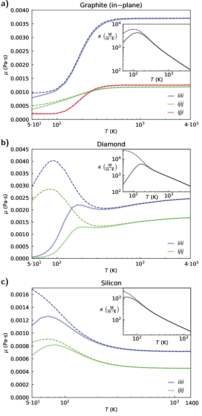
Figure 1: Largest components of the 4^th-order thermal viscosity tensor for graphite (a), diamond (b), and silicon (c), as a function of temperature (the off-plane tensor components for graphite are reported in Fig. 9). Insets: total thermal conductivities (in-plane components for graphite and diagonal components of the isotropic tensor for diamond and silicon) as a function of temperature. The dashed lines refer to the bulk materials (Eq. (9) for viscosity and Eq. (49) for conductivity); the solid lines show finite-size predictions computed using Eq. (54) and Eq. (55) for a sample having size (or grain size) $10\;\mu m$ (see main text and Appendix C; for diamond and silicon the component $\mu^{ijji}$ is negligible).

We report in Fig. 1 the first-principles estimates of the thermal viscosity for graphite, diamond, and silicon. We choose these three materials as prototypes for two different behaviors, the former two displaying hydrodynamic thermal transport Fugallo et al. (2013); Khodusov and Naumovets (2012); Fugallo et al. (2014); Ding et al. (2018); Huberman et al. (2019); Gandolfi et al. (2019), as opposed to the more conventional case of silicon Fugallo et al. (2013); Cepellotti and Marzari (2016). We account for finite-size effects by combining the bulk viscosity in Eq. (9) with its ballistic limit via Matthiessen’s rule for a sample having size (or grain size) of 10 $\mu m$; the same renormalization is applied also to the thermal conductivity (see Appendix C for details). This is an approximate treatment of surface scattering effects, which provides an estimate of size effects at a much lower computational complexity compared to more refined models Fugallo et al. (2014); Torres et al. (2017). In general, when samples’ sizes become comparable or smaller than the carriers’ diffusion lengths Heron et al. (2009); Siemens et al. (2010); Johnson et al. (2013); Regner et al. (2013); Wilson and Cahill (2014); Ziabari et al. (2018), transport coefficients cannot be rigorously defined and a more accurate treatment is required, solving the much more complex and computationally expensive space-dependent LBTE Péraud and Hadjiconstantinou (2011); Hua and Minnich (2014); Carrete et al. (2017); Cepellotti and Marzari (2017a). Matthiessen’s approach is a good approximation when the values of thermal conductivity and viscosity do not differ significantly from their bulk counterparts, as is the case for the materials, sizes and temperatures considered in this work (e.g., in Fig. 1 the size renormalization is negligibly small in the temperature range considered for graphite and silicon, and becomes so above 300 K for diamond).

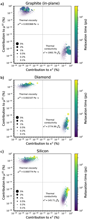
Figure 2: Relaxons’ contributions to the bulk thermal conductivity and to the thermal viscosity at 300 K for graphite (a, in-plane components), diamond (b) and silicon (c). Each dot represents a relaxon, with its color labeling its relaxation time, and its area being proportional to the sum of its percentage contributions to the thermal conductivity and viscosity. The dashed lines are plotted as a guide to the eye, to underscore how even and odd relaxons are fully decoupled. Odd relaxons, which determine the thermal conductivity, yield negligible (zero) contributions to the thermal viscosity; conversely, even relaxons determine the thermal viscosity and yield negligible (zero) contributions to thermal conductivity.

For graphite in the low-temperature ($\lesssim$100 K) regime, the bulk in-plane viscosity components are constant or slowly increasing with temperature; at higher temperatures, the viscosity components increase with temperature up to reaching their saturation values. For a graphite polycrystalline sample with a grain size of $10\mu m$, finite-size effects on viscosity (and on conductivity) are small. For diamond in the temperature regime below 90 K, the bulk values of the thermal viscosity increase with increasing temperature, then in the intermediate temperature regime ($100\;{\rm K}\lesssim T\lesssim 300\;{\rm K}$) they decrease with temperature, and finally for increasingly higher temperatures they gently increase up to saturating to the high-temperature limiting values. However, size effects renormalize this behavior for temperatures below 300 K, leaving viscosity components that increase with temperature. In silicon, increasing temperature yields a decrease, up to a high-temperature saturation value, of the bulk thermal viscosity; size effect renormalize the viscosity below $\sim 100$ K yielding viscosity components that increase with temperature (i.e. a behavior analogous to that of diamond). We note that in the high-temperature limit, i.e. when the thermal conductivity decay as $T^{-1}$ Ziman (1960); Sun and Allen (2010), the viscosity components tend to constant values for all these three materials. The total bulk thermal conductivities are shown in the insets of Fig. 1 for comparison (we only show one component; for diamond and silicon the conductivity tensor is isotropic, for graphite we show the in-plane component). The off-plane transport coefficients for graphite are discussed in Fig. 9a. In graphite, the bulk thermal conductivity below 100 K does not increase monotonically as the temperature is decreased due to the presence of natural-abundance isotopic scattering. Natural-abundance isotopic scattering has been considered also for diamond and silicon, and the thermal conductivity at low temperatures is much lower than for isotopically-pure diamond Fugallo et al. (2013); Berman (1992); Onn et al. (1992); Olson et al. (1993); Wei et al. (1993); Ward et al. (2009); Broido et al. (2012) or silicon Inyushkin et al. (2018). We have also verified that the effects of phonon coherences are negligible in these crystals Simoncelli, M. and Marzari, N. and Mauri, F. (2019). We note in passing that, even if the thermal conductivities of diamond and silicon differ by more than one order of magnitude, their largest thermal-viscosity components differ only by a factor of 3. These results may be compared with the case of water, whose dynamic (shear) viscosity is $8.5{\cdot}10^{-3}$ Pa$\cdot$s at room temperature, indicating that the thermal viscosity found here is comparable or larger. To a good approximation, water is an incompressible fluid, and thus its largest viscosity component is $ijij$, also called “first viscosity” or “shear viscosity”. For compressible fluids, the $iiii$ components of the viscosity tensor — also called “second viscosity” or “volume viscosity” Lifshitz and Pitaevskii (1981) — are non-negligible. Here, in contrast with water, the $iiii$ component of the thermal viscosity tensor is the largest, which elicits an analogy to a compressible fluid. It is important to mention that the present formulation may need further extension to deal with unstrained 2D materials, since their flexural phonon modes have a quadratic dispersion $\omega_{\nu}\propto q^{2}$ at $T=0K$ Bonini et al. (2012). Under these conditions, long-wavelength phonons lead to $\bm{q}\cdot\bm{u}$ being larger than $\omega_{\nu}$, causing negative values of the phonon drifting distribution which are not compatible with a semiclassical description of transport. Further work is needed to address this issue, for example considering the phonon renormalization due to coupling between bending and stretching degrees of freedom of the monolayer Mariani and von Oppen (2008) or the presence of a substrate Ong and Pop (2011), or introducing the Wigner-function formalism Simoncelli, M. and Marzari, N. and Mauri, F. (2019); Weinbub and Ferry (2018).

Finally, it is worth checking the complementary character of the thermal conductivity and viscosity that arises from their decoupled relaxons’ contributions. As commented above, decomposing the thermal conductivity Cepellotti and Marzari (2016) and viscosity (9) in terms of single relaxons it is possible to show that the thermal viscosity is uniquely determined by the even part of the relaxon spectrum, while the thermal conductivity is determined uniquely by the odd part of the relaxon spectrum Cepellotti and Marzari (2016). In Fig. 2 we highlight the contributions of each relaxon to the total thermal conductivity and viscosity, confirming numerically this picture.

III Viscous heat equations

We show here that heat conduction can be described by two novel viscous heat equations that cover on the same footing both the Fourier and hydrodynamic limits, and all intermediate regimes. These are two coupled equations in the temperature $T(\bm{r},t)$ and drift-velocity $\bm{u}(\bm{r},t)$ fields, which are parametrized by the thermal viscosity and conductivity. These equations represent the thermal counterpart of the Stokes equations of fluid dynamics — i.e. the Navier-Stokes equations in the linear regime, whose solution yields the laminar flow — where temperature takes the role of pressure and the phonon drift velocity that of the fluid velocity. In the kinetic regime, when momentum-dissipating (Umklapp) scattering processes dominate Cepellotti et al. (2015), these viscous heat equations become equivalent to Fourier’s heat equation.

As underscored before, hydrodynamic thermal transport is characterized by energy conservation and crystal momentum quasi-conservation (the latter being exactly conserved only in absence of Umklapp processes Sussmann and Thellung (1963)). Conserved quantities in the LBTE dynamics can be related to the eigenvectors of the full or normal scattering matrix with zero eigenvalues Hardy (1970) (see also Appendix A). Four of these eigenvectors (i.e. phonon distribution functions) can be identified. The first one is the Bose-Einstein eigenvector $\phi^{0}_{\nu}\propto\hbar\omega_{\nu}\propto\frac{\partial\bar{N}_{\nu}}{\partial T}\propto\tilde{n}^{T}_{\nu}$, which is the eigenvector of zero eigenvalue for the symmetrized full scattering matrix $\tilde{\Omega}_{\nu{\nu^{\prime}}}$; its zero eigenvalue is associated to energy conservation in scattering events (both normal and Umklapp). The other three eigenvectors are the drift eigenvectors $\phi_{\nu}^{i}\propto\hbar q^{i}\propto\frac{\partial N^{D}_{\nu}}{\partial u^{i}}\propto n^{D}_{\nu}$, $i=1,2,3$ (where $3$ is the dimensionality of the system) already introduced for the evaluation of the viscosity; these $\phi_{\nu}^{i}$ are eigenvectors with zero eigenvalue for the normal part of the scattering matrix $\tilde{\Omega}^{N}_{\nu{\nu^{\prime}}}$ and are associated to the conservation of crystal momentum by normal scattering events Sussmann and Thellung (1963); Guyer and Krumhansl (1966a); Hardy (1970). We note that these four eigenvectors constitute the first two terms of the phonon distribution expansion in Eq. (4). We can thus derive the mesoscopic equations that govern the evolution of the temperature ($T(\bm{r},t)$) and drift velocity ($\bm{u}(\bm{r},t)$) fields projecting the microscopic LBTE in the subspaces spanned by $\phi^{0}_{\nu}$ and by $\phi_{\nu}^{i}$ ($i=1,\dots,3$). In order to derive a closed-form equation for the drift velocity, when projecting in the subspace spanned by $\phi_{\nu}^{i}$ we consider the effects of momentum dissipation only within that subspace. The result is the following set of equations (see Appendix D for a detailed derivation):

$$C\frac{\partial T(\bm{r},t)}{\partial t}+\sum_{i,j=1}^{3}W_{0j}^{i}\sqrt{\bar{T}A^{j}C}\frac{\partial u^{j}(\bm{r},t)}{\partial r^{i}}-\sum_{i,j=1}^{3}\kappa^{ij}\frac{\partial^{2}T(\bm{r},t)}{\partial r^{i}\partial r^{j}}=0\;,$$ (10)

$$A^{i}\frac{\partial u^{i}(\bm{r},t)}{\partial t}+\sqrt{\frac{CA^{i}}{\bar{T}}}\sum_{j=1}^{3}{W}_{i0}^{j}\frac{\partial T(\bm{r},t)}{\partial r^{j}}-\sum_{j,k,l=1}^{3}\mu^{ijkl}\frac{\partial^{2}u^{k}(\bm{r},t)}{\partial r^{j}\partial r^{l}}=-\sum_{j=1}^{3}\sqrt{A^{i}A^{j}}{D}_{U}^{ij}u^{j}(\bm{r},t)\;,$$ (11)

where $C=\frac{1}{k_{B}\bar{T}^{2}V}\sum_{\nu}\bar{N}_{\nu}\big{(}\bar{N}_{\nu}+1\big{)}(\hbar\omega_{\nu})^{2}$ is the specific heat, ${W}_{0j}^{i}=\frac{1}{V}\sum_{\nu}\phi_{\nu}^{0}{v}^{i}_{\nu}\phi_{\nu}^{j}$ is a velocity tensor that arises from the non-diagonal form of the diffusion operator in the basis of the eigenvectors of the normal part of the scattering matrix (see Appendix D), $\bar{T}$ is the reference (equilibrium) temperature on which a perturbation is applied (see Sec. V and Appendix A.1), $A^{i}$ is the specific momentum in direction $i$ (defined in Sec. II), $\mu^{ijkl}$ is the thermal viscosity tensor, $\kappa^{ij}$ is the thermal conductivity tensor Cepellotti and Marzari (2016), and ${D}_{U}^{ij}=\frac{1}{V}\sum_{\nu{\nu^{\prime}}}\phi^{i}_{\nu}\tilde{\Omega}_{\nu{\nu^{\prime}}}^{U}\phi^{j}_{{\nu^{\prime}}}$ is the momentum dissipation rate; the latter is caused both by the presence of Umklapp processes as well as boundary scattering (i.e. ${D}_{U}^{ij}$ is sensitive to size effects like the thermal conductivity and viscosity). Treating boundary scattering as in Ref. Fugallo et al. (2014), we compute ${D}_{U}^{ij}$ as ${D}_{U}^{ij}={D}_{U,{\rm bulk}}^{ij}+{D}_{U,{\rm boundary}}^{ij}(L_{S})$, where ${D}_{U,{\rm bulk}}^{ij}=\frac{1}{V}\sum_{\nu{\nu^{\prime}}}\phi^{i}_{\nu}\tilde{\Omega}_{\nu{\nu^{\prime}}}^{U}\phi^{j}_{{\nu^{\prime}}}$ is the momentum dissipation caused by Umklapp scattering in the bulk and ${D}_{U,{\rm boundary}}^{ij}(L_{S})=\frac{1}{V}\sum_{\nu{\nu^{\prime}}}\phi^{i}_{\nu}\frac{|\bm{v}_{\nu}|\delta_{\nu,{\nu^{\prime}}}}{L_{S}}\phi^{j}_{{\nu^{\prime}}}$ is the momentum dissipation caused by scattering with boundaries at a distance $L_{S}$. The scalar equation (10) and the vectorial (3-components) equation (11) rule the coupled evolution of the scalar temperature field and of the vector drift-velocity field; they constitute the main result of this work and we name these “viscous heat equations”. These transport equations are reminiscent of the linearized Stokes equations for fluids: to see this more clearly, we note that local energy $E(\bm{r},t)$ and crystal momentum $\bm{P}(\bm{r},t)$ are proportional to temperature and drift velocity respectively ($E(\bm{r},t)=C\;T(\bm{r},t)$ and ${P}^{i}(\bm{r},t)=A^{i}\;{u}^{i}(\bm{r},t)$, where $C$ is the specific heat and $\bm{A}$ is the specific momentum). Exploiting these relationships, it is possible to rewrite the viscous heat equations in a more familiar form, namely as energy $E$ and momentum $P^{i}$ balance equations:

$$\frac{\partial E(\bm{r},t)}{\partial t}+\nabla\cdot\Big{(}\bm{Q}^{\delta}(\bm{r},t)+\bm{Q}^{D}(\bm{r},t)\Big{)}=0\;,$$ (12)

$$\frac{\partial P^{i}(\bm{r},t)}{\partial t}{+}\sum_{j}\left(\frac{\partial\Pi_{T}^{ij}(\bm{r},t)}{\partial r^{j}}+\frac{\partial\Pi_{\delta{\rm E}}^{ij}(\bm{r},t)}{\partial r^{j}}\right)=-\frac{\partial P^{i}(\bm{r},t)}{\partial t}\bigg{|}_{\text{Umkl}},$$ (13)

where, on the basis of the phonon population expansion in Eq. (4), we distinguish the drifting heat flux into the contributions from the local temperature gradient ${Q}^{\delta,i}(\bm{r},t)=-\sum_{j}\kappa^{ij}\nabla^{j}T(\bm{r},t)$ and from the drift velocity field ${Q}^{D,i}(\bm{r},t)=\sum_{j}W_{0j}^{i}\sqrt{\bar{T}A^{j}C}{u}^{j}(\bm{r},t)$. Similarly, the momentum flux receives separate contributions from the local temperature $\Pi^{ij}_{T}(\bm{r},t)=\sqrt{CA^{i}/\bar{T}}\;{W}_{i0}^{j}T(\bm{r},t)$ and from variations of the drift velocity through Eq. (8). Finally, $\frac{\partial P^{i}}{\partial t}\big{|}_{\text{Umkl}}$ accounts for the dissipation of crystal momentum by Umklapp processes or scattering with boundaries; further details can be found in Appendix D. The distinction between temperature-driven and drifting components of the heat flux ($\bm{Q}^{\delta}(\bm{r},t)$ and $\bm{Q}^{D}(\bm{r},t)$, respectively) is essential for hydrodynamic transport. We will show in Sec. VI that Fourier’s law is recovered in the limiting case where crystal momentum dissipation dominates over viscous effects and is the fastest timescale of the phonon dynamics.

It is worth mentioning that the viscous heat equations introduced here differ from the Stokes equations for fluids in two major ways. First, there is no analogous to the mass conservation satisfied by Stokes equations, since the total phonon number is not a constant of motion (e.g. a phonon coalescence event decreases the number of phonons in the system). Second, while collisions between molecules in the fluid conserve momentum, scattering among phonons does not conserve crystal momentum in presence of Umklapp processes.

The most relevant feature of the viscous heat equations is their capability to describe hydrodynamic thermal transport in terms of mesoscopic quantities, i.e. temperature and drift velocity, resulting in a much simpler and computationally less expensive approach than the microscopic LBTE. The parameters entering Eqs. (10, 11) can be determined from first-principles calculations or, possibly less accurately, from classical potentials, and are tabulated in Appendix E for graphite, diamond and silicon.

In order to be solved, the viscous heat equations require appropriate boundary conditions on the temperature and drift velocity. Boundary conditions on temperature have been widely studied in conjunction with Fourier’s heat equation Logan (2014): typically, one makes assumptions on the system’s capability to exchange heat at the boundaries, and on the temperature at those boundaries (Neumann and Dirichlet boundary conditions, respectively Logan (2014)). In the next section V we consider a system in which the temperature is fixed at some boundaries, while the others are assumed to be adiabatic (that is, the heat flux across these boundaries is zero). In contrast, boundary conditions on the drift velocity, i.e. on crystal momentum at the sample’s borders, have not been studied as extensively. Since crystal momentum is not conserved at boundaries Sussmann and Thellung (1963), we impose a no-slip condition of zero drift velocity $\bm{u}(\bm{r},t)$ on all boundaries, ensuring thus zero drifting heat $\bm{Q}^{D}(\bm{r},t)\propto\bm{u}(\bm{r},t)$. As discussed in past work Ziman (1960); Cepellotti and Marzari (2017a), more comprehensive boundary conditions require quantifying phonon reflection at surfaces, and are beyond the scope of this work.

The viscous heat equations (10,11) improve upon past work on different levels. First, they are valid for general dispersion relations for phonons, and thus overcome the limitations — pointed out by Hardy and Albers Hardy and Albers (1974) already in 1974 — of the pioneering mesoscopic models developed in the 1960s by Guyer-Krumhansl Guyer and Krumhansl (1966a, b) or Gurzhi Gurzhi (1968), which assumed linear-isotropic or power-law phonon dispersion relations, respectively (assumptions which arose from the hypothesis that hydrodynamic phenomena would occur at cryogenic temperatures only). The limitations of the Guyer-Krumhansl Guyer and Krumhansl (1966a, b) and Gurzhi Gurzhi (1968) models were overcome in 1974 by Hardy and Albers Hardy and Albers (1974), who derived from the LBTE a set of mesoscopic equations for energy and crystal momentum valid for a general phonon dispersion relation (i.e. not necessarily linear-isotropic). Hardy and Albers’ formulation relies on the hydrodynamic approximation — i.e. that the fastest timescale of phonon dynamics is that of normal processes — that is valid only within the hydrodynamic regime, where Umklapp collisions are rare events. In fact, Hardy and Albers’ equations are limited just to the hydrodynamic regime and do not incorporate Fourier’s law as a limit (and thus any intermediate regimes). The viscous heat equations address exactly this issue, and Fourier’s law emerges when crystal momentum dissipation (due to Umklapp processes or scattering with boundaries) dominates over viscous effects and is the fastest timescale of the phonon dynamics (see Sec. VI). Finally, the viscous heat equations take into account the entire collision matrix, at variance with recent mesoscopic models derived from the LBTE either in the SMA Guo and Wang (2018) or in the Callaway approximation Li and Lee (2018).

IV Second sound

Second sound is the coherent propagation of a temperature wave Sussmann and Thellung (1963); Guyer and Krumhansl (1966b); Kwok (1967); Enz (1968); Ackerman and Guyer (1968); Hardy (1970); Maris (1981a); Cepellotti and Marzari (2017b); Huberman et al. (2019); Chester (1963), and it is an effect properly described by the viscous heat equations. From a phenomenological point of view, second sound appears when the temperature field satisfies the following damped wave equation Hardy (1970) (we define $x$ as the second sound propagation direction):

$$\frac{\partial^{2}T(x,t)}{\partial t^{2}}+\frac{1}{\tau_{ss}}\frac{\partial T(x,t)}{\partial t}-v_{ss}^{2}\frac{\partial^{2}T(x,t)}{\partial x^{2}}=0\;,$$ (14)

where $\tau_{ss}$ and $v_{ss}$ are the second-sound relaxation time and undamped propagation velocity, yet to be determined. In contrast to Fourier’s law, which has the form of a classical (non-relativistic) diffusion equation and states that a temperature-gradient variation causes an instantaneous variation of the heat flux, Eq. (14) has the physical property that a sudden localized change of temperature propagates in space with a finite speed (i.e. it is not felt instantly everywhere in space) Cattaneo (1948); Joseph and Preziosi (1989); Tzou (1995); Bergamasco et al. (2018). The temperature profile that solves Eq. (14) has the form of a damped wave:

$$T(x,t)=\bar{T}+\delta T\;e^{i(kx-\bar{\omega}(k)t)}e^{-t/\tau_{ss}}\;,$$ (15)

where the second sound frequency $\bar{\omega}(k)$ depends on the second-sound wavevector $k$. In Appendix F we derive the second-sound equation from the viscous heat equations (10,11) following two different approaches (bottom-up and top-down). In the first bottom-up approach we find the conditions for which the damped wave equation (14) emerges form the viscous heat equations Eq. (10,11). When this happens, the solution of Eq. (14) is the damped wave equation for temperature (15) shown above, with the second-sound dispersion relation given by $\bar{\omega}(k)=\sqrt{v_{ss}^{2}k^{2}-(2\tau_{ss})^{-2}}$ (this can be easily verified substituting Eq. (15) into Eq. (14)). This allows to express $\tau_{ss}$ and $v_{ss}$ in terms of the parameters appearing in the viscous heat equations; in particular, $\tau_{ss}=\frac{C({W}_{x0}^{x})^{2}}{\kappa({D}^{xx}_{U})^{2}+{D}^{xx}_{U}C({W}_{x0}^{x})^{2}}$ and $v_{ss}=\frac{\kappa{D}^{xx}_{U}+C({W}_{x0}^{x})^{2}}{C{W}_{x0}^{x}}$. The propagation velocity of second sound is affected by damping and depends on the wavevector $k$: it is given by the group velocity $v_{g}(k)=\frac{\partial\bar{\omega}(k)}{\partial k}=kv_{ss}[k^{2}+(2\tau_{ss}v_{ss})^{-2}]^{-\frac{1}{2}}$, and we note that it reduces to the undamped propagation velocity $v_{ss}$ in the undamped limit $\tau_{ss}\to 0$.

These results are consistent with empirical expectations on second sound: in the limit of weak crystal momentum dissipation the second-sound relaxation time increases, while the velocity becomes smaller, making second sound more likely to be observed in the hydrodynamic regime Guyer and Krumhansl (1966b); Hardy (1970). In fact, when $D^{xx}_{U}\to 0$ we find that $\tau_{ss}\to({D}^{xx}_{U})^{-1}$ and $v_{ss}\to W^{x}_{x0}$. We note that the viscous heat equations describe not only the propagation of the temperature field, but also that of the drift velocity. In Appendix F we show that when second sound emerges the drift-velocity field propagates as a damped wave as well (i.e. similar to Eq. (15)), with the same relaxation time and velocity of temperature, but with a phase shift of $\pi/2$. Phase shifts between hydrodynamic and resistive components of the frequency-dependent heat flux have also been discussed recently in the context of an improved Callaway approximation for the LBTE Allen (2013).

As an alternative, we took inspiration from Ref. Cepellotti and Marzari (2017b), which derived the second-sound dispersion relations by taking advantage of the Laplace transform of the LBTE, to identify solutions in the form of a damped wave following a top-down approach. In particular, we take a damped-wave ansatz for temperature, Eq. (15), and a similar one for the drift-velocity field (with the same frequency and decay time of temperature); we substitute these into the viscous heat equations (10,11) and determine the conditions under which these are acceptable solutions. As detailed in Appendix F, we find that the dispersion relations of second sound in the long-wavelength limit reduce to $\omega(k)-\frac{i}{\tau_{ss}}\approx-\frac{iD_{U}^{xx}}{2}+\sqrt{-\bigg{(}\frac{D_{U}^{xx}}{2}\bigg{)}^{2}+k^{2}\bigg{(}W^{2}-\frac{D_{U}^{xx}\kappa}{C}-\frac{2\mu D_{U}^{xx}}{A}\bigg{)}}$. In this long wavelength limit and in the hydrodynamic regime $D_{U}\to 0$ we have $\tau_{ss}\approx\frac{1}{D_{U}^{xx}}$ and $v_{g}(k)\approx W$, which is consistent with the first bottom-up approach presented to derive the equations for second sound. We further stress that the LBTE can only rigorously describe second sound in the long-wavelength limit $k\to 0$ in order for the temperature to be slowly varying (for which the two approaches shown in this section provide the same result); for smaller wavelengths, the definition of temperature itself becomes questionable Lepri et al. (2003).

We also recall that Enz Enz (1968) and Hardy Hardy (1970) distinguished between “drifting” and “driftless” second sound. The former emerges when normal processes dominate and is described in terms of balance equations for energy and momentum; the latter is determined by a uniform energy flux that decays exponentially. The second sound discussed here is of the drifting kind, as it emerges from a set of balance equations for energy and crystal momentum derived from the LBTE.

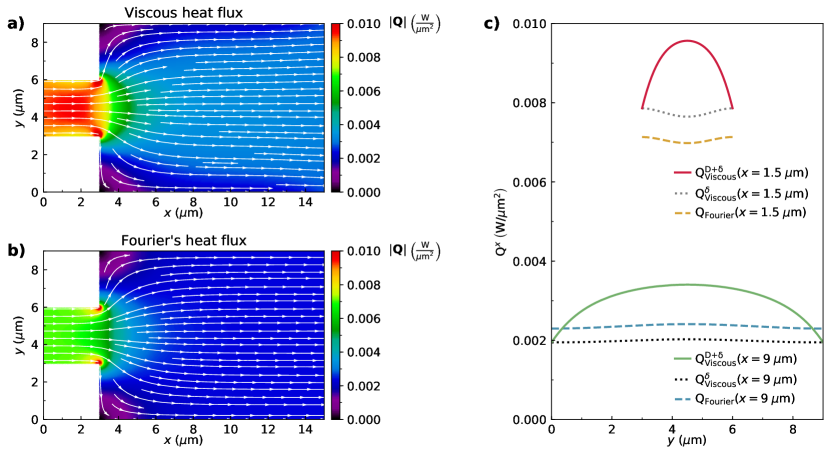
Figure 3: In-plane ($x-y$) heat fluxes in graphite around $\bar{T}=70$ K, for a sample infinite in the $z$ direction (the $z$ direction of the sample coincides with the off-plane direction of graphite). Panel a) shows the total heat flux (${\bm{Q}}^{D}+{\bm{Q}}^{\delta}$) obtained from the viscous heat equations (10, 11). Panel b) shows instead the Fourier heat flux (${\rm Q}^{i}_{\rm Fourier}(\bm{r},t){=}-\sum_{j}\kappa^{ij}\nabla^{j}T(\bm{r},t)$) obtained solving the steady-state Fourier equation $\sum_{ij}\kappa^{ij}\frac{\partial^{2}T(\bm{r},t)}{\partial r^{i}\partial r^{j}}=0$. Boundary conditions are as follows: the temperature is set at 80K/60K on the left/right boundaries, a zero total heat flux is imposed at the other boundaries, and zero drift velocity is imposed on all boundaries (no-slip boundary condition). With this choice of boundary conditions, the phonon distribution reduces to the Bose-Einstein distribution on the left/right boundaries, where the temperature is fixed. Despite having local equilibrium at the left/right boundaries, a non-zero drift velocity is present in the material as a consequence of the coupling in Eq. (10) between drift velocity and temperature. Panel c) shows the $x$-component of the heat flux along sections taken at $x=1.5\;\mu m$ (orange, gray, red) and $x=9.0\;\mu m$ (black, blue, green); solid lines are the results obtained from the viscous heat equations, dashed lines are the results from Fourier’s law, and dotted lines are the heat fluxes due to the temperature gradient within the viscous heat equations ($\bm{Q}^{\delta}$).

V Case study

We showcase the solution for the viscous heat equations for graphite around the equilibrium temperature $\bar{T}=70$ K in the geometry shown in Fig. 3, often used as an illustrative example in textbooks on fluid dynamics. The equations are solved numerically using a finite-element solver implemented in Mathematica Inc. (2016), imposing a temperature of 80 K on the left side ($x=0\;\mu m$) and of 60 K on the right side ($x=15\;\mu m$), assuming all boundaries at $x\neq 0$ and $x\neq 15\;\mu m$ to be adiabatic, and imposing a no-slip condition on $\bm{u}$ at all boundaries.

We show in Fig. 3 the viscous heat flux $\bm{Q}^{\delta}+\bm{Q}^{D}$, and the flux predicted by Fourier’s law $\bm{Q}_{\rm Fourier}$ (left panels) and contrast the Fourier and viscous heat flux components across two different sections (right panel).

We stress that Fourier’s law lacks a description of the contribution to the heat flux derived from the local drift velocity Sussmann and Thellung (1963); Maris (1981b); Simons (1983). As a result, Fourier’s law misses qualitative and quantitative properties of the heat flux profile. The largest differences are observed in proximity of spatial inhomogeneities, such as boundaries or corners. For example, $\bm{Q}^{D}$ quickly increases (decreases) in proximity of the thermal reservoir on the hot-left (cold-right) side of the sample; these changes in $\bm{Q}^{D}$ determine opposite changes in $\bm{Q}^{\delta}$. Microscopically, these variations are caused by the rapid transition of the phonon distribution from the Bose-Einstein equilibrium distribution imposed at the boundaries to an out-of-equilibrium distribution carrying non-zero total crystal momentum (i.e. a drift velocity) inside the sample.

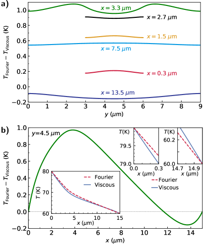
Figure 4: Difference between the temperature profiles predicted by Fourier’s law and by the viscous heat equations, plotted in the top panel a) along $y$ for various values of $x$ and in the bottom panel b) along $x$ for $y=4.5\;\mu m$. The insets of panel b) show the temperature profile along $x$ for $y=4.5\;\mu m$; the result of the viscous heat equations (10, 11) is solid/blue, Fourier’s law prediction is dashed/red.

We report in Fig. 3c the total heat flux profiles along two transversal sections of the sample, contrasting the prediction from the viscous heat equations (solid lines) with that of Fourier’s law (dashed lines). Along these sections, Fourier’s law predicts a flat heat flux profile, while the viscous heat equations yield a Poiseuille-like profile. The results from the viscous heat equations are thus substantially different from Fourier’s predictions, and the behavior of the heat flux can be understood from a simple analytical 1D solution of the viscous heat equations in the absence of Umklapp processes Sussmann and Thellung (1963): as discussed in Appendix G, the flux is described by hyperbolic functions with a characteristic length scale $b=\sqrt{\frac{\mu\kappa}{AC(W)^{2}}}$ (an estimate of the friction lengths, see Ref. Cepellotti and Marzari (2017a)). At distances from the surface larger than $b$ we recover the flat behavior typical of the bulk. We also note that these results mimic those from the (computationally very expensive) space-dependent solution of the LBTE (either in the frequency-dependent SMA approximation Péraud and Hadjiconstantinou (2011) or considering the full scattering operator Cepellotti and Marzari (2017a)), which generates a minimum flux on surfaces and maximum at the sample’s center. We further note that, at variance with classical fluid dynamics and as pointed out in Ref. Cepellotti and Marzari (2017a), the total heat flux does not drop to zero at the boundaries: the no-slip condition sets the drifting heat flux $\bm{Q}^{D}$ to zero, but the temperature-driven component $\bm{Q}^{\delta}$ is still allowed to be nonzero.

In Fig. 4 we plot the difference between the temperature profile predicted by Fourier’s law and the viscous heat equations along longitudinal (top panel) and transversal (bottom panel) directions. The insets in Fig. 4b show the results of the viscous equations (solid blue line) and Fourier’s law (dashed red line) along the section $y=4.5\;\mu m$. Along the transversal direction (Fig. 4a), Fourier’s law and Eqs. (10, 11) predict temperature profiles which are substantially different in the presence of variations of the sample’s shape (green line corresponding to $x=3.3\;\mu m$), while they are merely shifted by a positive or negative offset away from these; the precise amount depends on the distance from the fixed-temperature boundaries. These differences become more clear by inspecting the longitudinal direction (Fig. 4b), where the discrepancy between the temperature predicted by Fourier’s law and Eqs. (10, 11) is largest at $x\simeq 3\;\mu m$, i.e. where the sample of Fig. 3 changes geometry. We show in the inset of Fig. 4b that also the longitudinal temperature profile (for $y=4.5\;\mu m$) changes when going from Fourier’s law (dashed red line) to the viscous heat equations (solid blue line). The difference is maximized close to variations of the sample’s shape at $x=3\;\mu m$ and at the boundaries $x=0$ and $x=15$ $\mu m$; in this latter case, the viscous heat equations predict steeper-than-Fourier’s law or non-linear temperature gradients that are reminiscent of those obtained in molecular dynamics simulations Schelling et al. (2002); Zhang et al. (2017); Khadem and Wemhoff (2013); Puligheddu et al. (2017); Iubini et al. (2018); He et al. (2012); Zhou et al. (2009); Fan et al. (2017); Allen (2018); Li et al. (2019) and in explicit solutions of the LBTE Cepellotti and Marzari (2017a).

VI Fourier Deviation Number

In this section, we introduce a descriptor that parametrizes the conditions under which hydrodynamic heat conduction is observed; we will refer to this as the “Fourier deviation number” (FDN). In particular, we aim at distinguishing the diffusive regime from the hydrodynamic regime: in the former case the viscous heat equations become equivalent to Fourier’s law, while in the latter case Fourier’s law no longer holds and the viscous heat equations are required.

In order to investigate how the hydrodynamic deviations from Fourier’s law depend on the sample’s sizes and reference temperature $\bar{T}$, we solve the viscous heat equations and Fourier’s equation for several samples having different dimensions, and at various reference temperatures $\bar{T}$. We perform this analysis for graphite (Fig. 5a), diamond (Fig. 5b) and silicon (Fig. 5c). In particular, we consider samples that are similar — in the geometric sense — to the reference sample shown in Fig. 3, i.e. we generate samples of different dimensions starting from the reference sample of Fig. 3 and varying the sizes via a uniform scaling. Following this protocol, we vary the sample’s length $l_{\rm TOT}$, reported on the $y-$axis of Fig. 5a-c, from $0.1$ to $100$ $\mu$m (e.g. the reference sample of Fig. 3 corresponds to $y=15\;\mu m$, $y=100\;\mu m$ corresponds to a sample obtained magnifying uniformly by a factor of $100/15\simeq 6.66$ the sizes of the reference sample). The color in Fig. 5a-c represents the normalized $\mathcal{L}^{2}$ distance between the temperature profile predicted by Fourier’s law and the viscous heat equations for a given sample length $l_{\rm TOT}$ and reference temperature $\bar{T}$:

$$\begin{split}{\mathcal{L}^{2}}[&{T}_{\rm Fourier}-{T}_{\rm Viscous}](l_{\rm TOT},\bar{T})=\\ &\sqrt{\frac{\int_{G}[T_{\rm Fourier}(x,y)-T_{\rm Viscous}(x,y)]^{2}dxdy}{\int_{G}dxdy}}\;,\end{split}$$ (16)

and in order to ease the qualitative interpretation of these results later, we evaluate $\mathcal{L}^{2}$ in the spatially-homogeneous region $G$ defined by $x>\frac{1}{5}l_{\rm TOT}$. We also inspected the effects of shape on the deviation $\mathcal{L}^{2}$, finding that the magnitude of $\mathcal{L}^{2}$ is larger for geometries with spatial non-homogeneities that imply larger values of the drift velocity’s second derivative; nevertheless, the dependence of $\mathcal{L}^{2}$ on $l_{\rm TOT}$ and $\bar{T}$ is qualitatively unchanged for different shapes.

Results in Figs. 5a-c have been computed accounting for finite-size effects as discussed in Sec. II and Appendix C. Additionally, to better compare with the experimental results of Ref. Huberman et al. (2019), we make the hypothesis of working with polycrystalline graphite with an average crystal grain size of $10\;\mu m$ as in Ref. Huberman et al. (2019): as a result, the transport coefficients of graphite are renormalized by the system size for $l_{\rm TOT}<10\;\mu m$, and by the grain size for $l_{\rm TOT}>10\;\mu m$ (therefore, for $l_{\rm TOT}>10\;\mu m$ size effects are given only by the boundary conditions effects on the temperature and drift-velocity fields). In graphite, the difference between Fourier’s law and the viscous heat equations is largest in the temperature range 60-80 K and for sizes $10\mu m\lesssim l_{\rm TOT}\lesssim 20\mu m$.

Turning our attention to diamond, we first recall that its thermal properties are characterized by a very large thermal conductivity, which originates from having large group velocities and weak Umklapp scattering Berman (1992); Onn et al. (1992); Olson et al. (1993); Wei et al. (1993); Ward et al. (2009); Broido et al. (2012); the latter condition being favorable to the emergence of hydrodynamic effects. This is confirmed by the results shown in Fig. 5b, with the hydrodynamic deviation being largest around room temperature and dimension $l_{\rm TOT}\gtrsim 1\;\mu m$ (we note in passing that, at this temperature and size, the surface-renormalization of transport coefficients is small and well compatible with the mesoscopic approach described in this work). These results suggest that a hydrodynamic window exists also for diamond, and that therefore hydrodynamic behavior (e.g. second sound) might be measurable in this material at temperatures even larger than graphite.

For silicon, instead, the deviation from Fourier’s law is smaller and takes place at lower temperatures. Silicon is an example of a material for which the thermal conductivity computed within the SMA approximation is very close to the conductivity computed from the exact solution of the LBTE Broido et al. (2007); Fugallo et al. (2013); Li et al. (2014); Cepellotti and Marzari (2016), and it is known that the SMA works reasonably well in systems where momentum-dissipating (Umklapp) scattering events dominate over those conserving crystal momentum (normal) Li et al. (2014); Lindsay (2016). Therefore, the negligible magnitude of hydrodynamic effects predicted by the viscous heat equations for silicon is consistent with the predominance of Umklapp over normal scattering events known to occur in this material. We last remark that, in contrast to graphite, results for diamond and silicon have been computed for single crystals, i.e. transport coefficients are not limited by grains’ size.

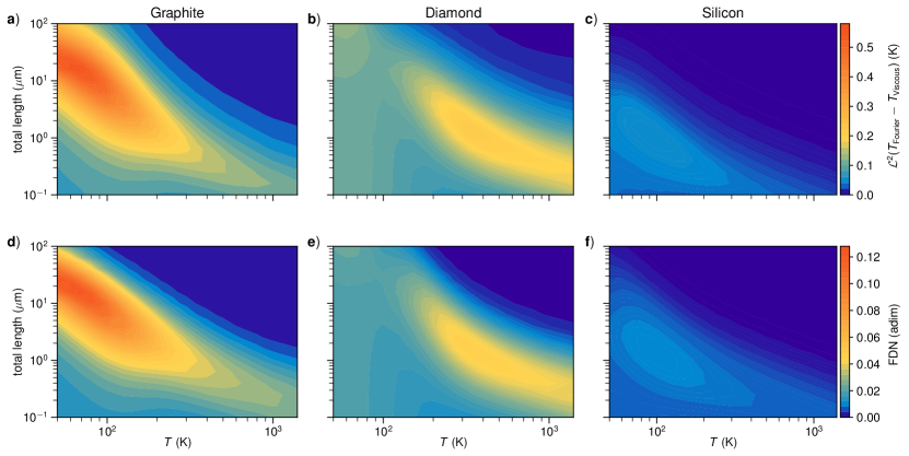
Figure 5: Top row, $\mathcal{L}^{2}$ distance (see text) between the temperature profile predicted by Fourier’s law and that of the viscous heat equations (10, 11), shown as a function of temperature and total length of a sample similar (in the geometric sense) to the shape of Fig. 3 for the cases of graphite (a), diamond (b) and silicon (c). The color quantifies the $\mathcal{L}^{2}$ distance between the temperature profiles predicted by Fourier’s law ($T_{\rm Fourier}(x,y)$) and the viscous heat equations (10, 11) ($T_{\rm Viscous}(x,y)$), computed over the region $G$ corresponding to points with $x>\frac{1}{5}l_{\rm TOT}$ where $l_{\rm TOT}$ is the total length of the sample geometrically similar to that in Fig. 3 (see main text for details). Bottom row, Fourier Deviation Number (FDN, as defined in Eq. (22)) for the same materials as a function of temperature and total length of the sample (for the geometry of Fig. 3, the characteristic size $L$ appearing in FDN is the shortest length-scale, i.e. 1/5 of the total length $l_{\rm TOT}$). It is apparent that the FDN correctly identifies the deviations between the solutions of the Fourier and of the viscous heat equations solutions.

In order to capture intuitively and inexpensively all these trends we introduce an approach inspired by the definition of the Reynolds number, and we rewrite the viscous heat equations (10, 11) in adimensional form (we follow the standard procedure used e.g. in fluid dynamics, which is also called “Buckingham Pi theorem” Buckingham (1914); White (2003)). First, we extract the magnitudes of the tensors appearing in the viscous heat equations, factorizing the largest component: $A^{i}{=}A_{\rm m}\mathsf{a}^{i}$, where $A_{\rm m}{=}\max\limits_{i}(|A^{i}|)$ and $\mathsf{a}^{i}=A^{i}/A_{\rm m}$ is an adimensional tensor with the largest component having modulus equal to $1$. Similarly, we factorize the largest component of all other tensors: $\kappa^{ij}{=}\kappa_{\rm m}\mathsf{k}^{ij}$ (with $\kappa_{\rm m}{=}\max\limits_{i,j}(|\kappa^{ij}|)$ and $\mathsf{k}^{ij}{=}\kappa^{ij}/\kappa_{\rm m}$); $W^{j}_{i0}{=}W_{\rm m}\mathsf{w}^{j}_{i}$ (with $W_{\rm m}{=}\max\limits_{i,j}(|W^{j}_{i0}|)$ and $\mathsf{w}^{j}_{i}{=}W^{j}_{i0}/W_{\rm m}$); $D^{ij}_{U}{=}D_{U,{\rm m}}\mathsf{d}^{ij}$ (with $D_{U,{\rm m}}{=}\max\limits_{i,j}(|D^{ij}_{U}|)$ and $\mathsf{d}^{ij}{=}D^{ij}_{U}/D_{U,{\rm m}}$); $\mu^{ijkl}{=}\mu_{\rm m}\mathsf{m}^{ijkl}$ (with $\mu_{\rm m}{=}\max\limits_{i,j,k,l}(|\mu^{ijkl}|)$ and $\mathsf{m}^{ijkl}{=}\mu^{ijkl}/\mu_{\rm m}$). Then, we define a set of dimensionless variables $\bm{r}^{*}=\bm{r}/L$, $\bm{u}^{*}=\bm{u}/u_{0}$, and $T^{*}=T/{\delta T}$, where $L$, $u_{0}$ and $\delta T$ are a characteristic size, drift velocity and temperature perturbation (more on these later). Substituting these variables in Eqs. (10, 11), and limiting ourselves to the steady-state regime, we obtain:

$$\pi_{1}\sum_{i,j=1}^{3}\frac{\mathsf{w}^{i}_{j}\sqrt{\mathsf{a}^{j}}}{g(\mathsf{w}{\cdot}\sqrt{\mathsf{a}})_{2}}\frac{\partial{u}^{*j}(\bm{r}^{*})}{\partial r^{*i}}-\sum_{i,j=1}^{3}\frac{\mathsf{k}^{ij}}{g(\mathsf{k})_{2}}\frac{\partial^{2}T^{*}(\bm{r}^{*})}{\partial r^{*i}\partial r^{*j}}=0\;,$$ (17)

$$\pi_{2}\sqrt{\mathsf{a}^{i}}\sum_{j=1}^{3}\frac{\mathsf{w}^{j}_{i}}{g^{i}(\mathsf{w})_{1}}\frac{\partial T^{*}(\bm{r}^{*})}{\partial r^{*j}}-\pi_{3}\sum_{j,k,l=1}^{3}\frac{\mathsf{m}^{ijkl}}{g^{i}(\mathsf{m})_{3}}\frac{\partial^{2}u^{*k}(\bm{r}^{*})}{\partial r^{*j}\partial r^{*l}}=$$

$$\hskip 99.58464pt-\sum_{j=1}^{3}\frac{\sqrt{\mathsf{a}^{i}\mathsf{a}^{j}}\mathsf{d}^{ij}}{g^{i}(\sqrt{\mathsf{a}{\otimes}\mathsf{a}}{\cdot}\mathsf{d})_{1}}{u}^{*j}(\bm{r}^{*})\;,$$ (18)

where we have introduced the quantities
$g(\mathsf{w}{\cdot}\sqrt{\mathsf{a}})_{2}=({\max_{ij}[\mathsf{w}^{i}_{j}\sqrt{\mathsf{a}^{j}}]})^{-1}\sum_{ij}{\mathsf{w}^{i}_{j}\sqrt{\mathsf{a}^{j}}}$,
$g(\mathsf{k})_{2}=({\max_{ij}[\mathsf{k}^{ij}]})^{-1}\sum_{ij}{\mathsf{k}^{ij}}$,
$g^{i}(\mathsf{w})_{1}=({\max_{j}[\mathsf{w}^{i}_{j}]})^{-1}\sum_{j}{\mathsf{w}^{i}_{j}}$,
$g^{i}(\sqrt{\mathsf{a}{\otimes}\mathsf{a}}{\cdot}\mathsf{d})_{1}=({\max_{j}[\sqrt{\mathsf{a}^{i}\mathsf{a}^{j}}\mathsf{d}^{ij}]})^{-1}\sum_{j}\sqrt{\mathsf{a}^{i}\mathsf{a}^{j}}\mathsf{d}^{ij}$,
$g^{i}(\mathsf{m})_{3}=({\max_{jkl}[\mathsf{m}^{ijkl}]})^{-1}\sum_{jkl}{\mathsf{m}^{ijkl}}$. The role of these parameters is to account for the correct order of magnitude of the five summations appearing in Eqs. (17,18); they carry a Cartesian superscript $i$ whenever they may depend on direction, and their subscripts indicate the number of indexes summed in their definition. For example, for a $3{\times}3$ isotropic tensor $\chi^{ij}=\chi_{\rm m}\delta^{ij}$ (where $\chi_{\rm m}$ is a constant and $\delta^{ij}$ is the Kronecker tensor), $g(\chi)_{2}=(\chi_{\rm m})^{-1}\sum_{ij}\chi^{ij}=3$ and $g^{i}(\chi)_{1}=(\chi_{\rm m})^{-1}\sum_{j}\chi^{ij}=1\;\forall\;i$. Because we are computing the FDN for the planar geometry discussed in Fig. 3, we can discard the $z$ component (i.e. the Cartesian direction indexed by $3$) from Eqs. (17,18). Then, for diamond, silicon and in-plane graphite, transport properties are isotropic (i.e. all the 2^nd-rank tensors appearing in Eq. (17) and Eq. (18) are diagonal). From this it follows that $g(\mathsf{w}{\cdot}\sqrt{\mathsf{a}})_{2}=2$; $g(\mathsf{k})_{2}=2$; $g^{i}(\mathsf{w})_{1}=1\;\forall\;i=1,2$; and $g^{i}(\sqrt{\mathsf{a}{\otimes}\mathsf{a}}{\cdot}\mathsf{d})_{1}=1\;\forall\;i=1,2$. Finally, the tensor $\mathsf{m}^{ijkl}$ is not isotropic (because the thermal viscosity tensor from which it is derived is not isotropic), and from the values in Fig. 1 it follows that $g^{i}(\mathsf{m})_{1}=1+\frac{\mu^{xyxy}}{\mu^{xxxx}}\forall i=1,2,3$ for diamond and silicon, and $g^{i}(\mathsf{m})_{1}=1+\frac{\mu^{xyxy}}{\mu^{xxxx}}+2\frac{\mu^{xyyx}}{\mu^{xxxx}}\;\forall\;i=1,2$ for graphite.

The final expressions for the dimensionless parameters $\pi_{1},\;\pi_{2},\;\pi_{3}$ are thus:

$$\pi_{1}=\frac{\sqrt{\bar{T}A_{\rm m}C}W_{\rm m}u_{0}L}{\kappa\cdot\delta T}\frac{g(\mathsf{w}{\cdot}\sqrt{\mathsf{a}})_{2}}{g(\mathsf{k})_{2}}\;,$$ (19)

$$\pi_{2}=\sqrt{\frac{C}{A_{\rm m}\bar{T}}}\frac{W_{\rm m}\delta T}{L{D}_{U,{\rm m}}u_{0}}\frac{g^{i}(\mathsf{w})_{1}}{g^{i}(\sqrt{\mathsf{a}{\otimes}\mathsf{a}}{\cdot}\mathsf{d})_{1}}\;,$$ (20)

$$\pi_{3}=\frac{\mu_{\rm m}}{{D}_{U,{\rm m}}L^{2}A_{\rm m}}\frac{g^{i}(\mathsf{m})_{3}}{g^{i}(\sqrt{\mathsf{a}{\otimes}\mathsf{a}}{\cdot}\mathsf{d})_{1}}\;.$$ (21)

From the derivation of these parameters, it is clear that they can be interpreted in terms of average values (we indicate with $\big{<}\dots\big{>}$ the average over space) of physical quantities: $\pi_{1}{\sim{\big{<}{Q}^{D}\big{>}}/{\big{<}Q^{\delta}\big{>}}}$, $\pi_{2}\sim{\big{<}\frac{\partial\Pi_{T}}{\partial r}\big{>}}/{\big{<}\frac{\partial P}{\partial t}\big{|}_{\text{Umkl}}\big{>}}$ and $\pi_{3}\sim{\big{<}\frac{\partial\Pi_{\delta{\rm E}}}{\partial r}\big{>}}/{\big{<}\frac{\partial P}{\partial t}\big{|}_{\text{Umkl}}\big{>}}$. Still, to evaluate these parameters we need to know the characteristic size $L$ and temperature perturbation $\delta T$, and estimate the characteristic values of the drift velocity $u_{0}$. Focusing on the setup discussed in the previous section (Fig. 3), we have $L=\frac{1}{5}l_{\rm TOT}$ (corresponding to the shortest length scale of the geometry considered, which has total length $l_{\rm TOT}$ along $x$) and $\delta T$=10K. As shown in Appendix H, the characteristic drift velocity $u_{0}$ is found by interpolating the asymptotic behavior at low ($u_{L}$) and high ($u_{H}$) temperatures $u_{0}^{-1}=u_{L}^{-1}+u_{H}^{-1}$. In the low-temperature limit, where Umklapp scattering is frozen, viscous effects determine the drift velocity, and one can show that $u_{L}=\frac{3}{7}\sqrt{\frac{CA}{\bar{T}}}\frac{{W}^{x}_{x0}\;\delta T\;L}{\mu^{xyxy}\left(1+\frac{\mu^{xxxx}}{\mu^{xyxy}}\right)}$ . In the high temperature limit, the drift velocity is mainly determined by the crystal momentum dissipation rate and $u_{H}=\sqrt{\frac{C}{\bar{T}A^{x}}}\frac{{W}_{x0}^{x}}{{D}_{U}^{xx}}\frac{2}{7}\frac{\delta T}{L}$. We can therefore estimate the values of all the $\pi_{1}$, $\pi_{2}$, and $\pi_{3}$ factors.

Looking at the definition of $\pi_{1}$, $\pi_{2}$ and $\pi_{3}$, it is straightforward to identify the conditions for which the viscous heat equations reduce to Fourier’s law. When $\pi_{3}{\ll}1$, i.e. for crystal momentum dissipation dominating over viscous effects and/or very large characteristic size $L$, the temperature gradient in Eq. (18) is proportional to the drift velocity: $\pi_{2}\sum_{j}\frac{\mathsf{w}^{j}_{i}}{g^{i}(\mathsf{w})_{1}}\frac{\partial T^{*}(\bm{r}^{*})}{\partial r^{*j}}{\simeq}-\sum_{j}\frac{\sqrt{\mathsf{a}^{j}}\mathsf{d}^{ij}}{g^{i}(\sqrt{\mathsf{a}{\otimes}\mathsf{a}}{\cdot}\mathsf{d})_{1}}{u}^{*j}(\bm{r}^{*})$. While it is intuitive to understand the emergence of Fourier’s law when crystal momentum dissipation (e.g. due to Umklapp scattering) dominates over viscous effects, the Fourier-like behavior of large-size samples can be rationalized qualitatively recalling the simple analytical 1D solution of the viscous heat equations in the absence of Umklapp processes discussed in Appendix G: the heat flux is described by hyperbolic functions with a characteristic length scale $b=\sqrt{\frac{\mu_{\rm m}\kappa_{\rm m}}{A_{\rm m}C(W_{\rm m})^{2}}}$, and for a characteristic size $L\gg b$, a flat Fourier-like heat flux profile is recovered. It is worth mentioning that $\pi_{3}\ll 1$ — and thus Fourier-like behavior — can also emerge for very small (sub-micrometer) length scales, where ballistic effects are relevant and strongly renormalize the transport coefficients, as discussed in Appendix C. The emergence of Fourier-like behavior in the ballistic regime (with a size-dependent thermal conductivity alike to that employed here) has been explained in a recent work Maassen and Lundstrom (2015), confirming that the results for sub-micrometer sizes obtained with the aforementioned approximated treatment of boundary scattering are qualitatively correct. If we insert the condition $\pi_{3}\ll 1$ in Eq. (17), we obtain a Fourier-like equation for the temperature: $\sum\limits_{i,j}\Big{[}\Big{(}\pi_{1}\pi_{2}\frac{g(\mathsf{k})_{2}g^{i}(\sqrt{\mathsf{a}{\otimes}\mathsf{a}}{\cdot}\mathsf{d})_{1}}{g(\mathsf{w}{\cdot}\sqrt{\mathsf{a}})_{2}g^{i}(\mathsf{w})_{1}}\sum\limits_{k,l}(\mathsf{w}^{i}_{k}\mathsf{d}^{-1})^{kl}\mathsf{w}^{j}_{l}\Big{)}{+}{\mathsf{k}^{ij}}\Big{]}\frac{\partial^{2}T^{*}(\bm{r}^{*})}{\partial r^{*i}\partial r^{*j}}{=}0$. So, the thermal conductivity is corrected by a term proportional to $\pi_{1}\pi_{2}$ (since in all the setups considered here, $\frac{g(\mathsf{k})_{2}g^{i}(\sqrt{\mathsf{a}{\otimes}\mathsf{a}}{\cdot}\mathsf{d})_{1}}{g(\mathsf{w}{\cdot}\sqrt{\mathsf{a}})_{2}g^{i}(\mathsf{w})_{1}}=1$), but the qualitative behavior is that of Fourier’s law. Numerically, we find that $\pi_{1}\pi_{2}{\ll}1$ for graphite in the high-temperature limit (see Fig. 6a), so that the viscous heat flux is well approximated by Fourier’s flux; the same limiting behavior is observed also in diamond and silicon. On the other hand, deviations from the temperature profile predicted by Fourier’s law appear when both $\pi_{1}$ and $\pi_{3}$ are large. In fact, $\pi_{3}\gtrsim 1$ implies that the temperature gradient in Eq. (18) is coupled to the second derivative of the drift velocity, and one can not obtain a Fourier-like equation as before; large values of $\pi_{1}$ imply that the drift velocity affects the evolution of temperature in Eq. (17). It follows that Fourier’s law is mathematically recovered for crystal momentum dissipation dominating over viscous effects and/or large characteristic size ($\pi_{3}{\ll}1$), but deviations between the viscous and Fourier temperature profile can be small even when viscous effects dominate over crystal momentum dissipation ($\pi_{3}{\gg}1$) if the coupling between drift velocity and temperature in Eq. (17) is small ($\pi_{1}{\ll}1$). We note in passing that while this reasoning has been made here at steady state, it can be straightforwardly extended to the time-dependent case, considering time variations of the drifting velocity slow compared to the crystal momentum dissipation timescale.

On the basis of this reasoning, it is convenient to introduce a Fourier deviation number (FDN) as:

$${\rm FDN}=\left(\frac{1}{\pi_{1}}+\frac{1}{\pi_{3}}\right)^{-1}\;,$$ (22)

which provides a simple estimate of the deviations from Fourier’s law: the larger the FDN, the larger the deviations from Fourier’s law.

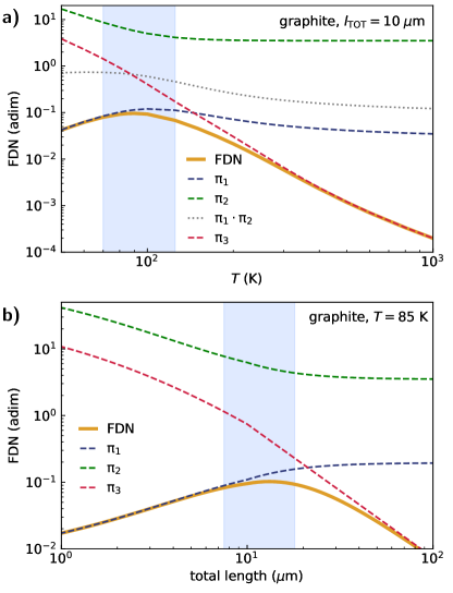
Figure 6: Fourier Deviation Number (FDN, solid line) and its different contributions $\pi_{1}$ and $\pi_{3}$ defined in Eq. (22) for a graphite sample of fixed length $l_{\rm TOT}=10\mu m$ as a function of temperature (panel a), and at fixed $T$=85 K as a function of sample’s length $l_{\rm TOT}$ (panel b). The shaded areas are the hydrodynamic (second-sound) windows measured at $10\mu$m (panel a) or 85 K (panel b) by Huberman et al. (2019). The terms $\pi_{2}$ and $\pi_{1}\pi_{2}$ are also reported in panel a) because in the high-temperature limit Fourier’s law is recovered when $\pi_{1}\pi_{2}\ll 1$ (see main text for details). Notably, FDN predicts hydrodynamic effects to be largest at temperatures and sizes that are in excellent agreement with these observed in the experiments.

In Fig. 5d-f, we plot the FDN for graphite, diamond and silicon as a function of sample’s total length $l_{\rm TOT}$ and reference temperature $\bar{T}$. Remarkably, the FDN captures the trends of the exact solution of the viscous heat equations (Fig. 5a-c), thus identifying accurately the regime where hydrodynamic behavior emerges. The magnitude of FDN is directly proportional to the magnitude of hydrodynamic effects: a larger FDN implies a larger difference between the Fourier and viscous temperature profiles. A detailed analysis of the $\pi$ terms as a function of temperature for a graphite sample geometrically similar to that in Fig. 3 and with a fixed total length $l_{\rm TOT}=10\mu$m is shown in Fig. 6a, where $l_{\rm TOT}=10\mu$m has been chosen to match the length fixed in the experiments by Huberman et al. (2019) to investigate the magnitude of hydrodynamic effects as a function of temperature. Importantly, the FDN at fixed $l_{\rm TOT}=10\mu$m predicts hydrodynamic effects to be largest at temperatures that match very well those measured in recent experiments for second sound in graphite Huberman et al. (2019). Then, we rationalize the trend of FDN as a function of temperature in terms of the $\pi$ terms entering in Eq. (22): $\pi_{1}$ increases with temperature for T$\lesssim 100$ K and saturates to a constant value at high temperature and $\pi_{3}$ decreases asymptotically like $T^{-2}$. Fig. 6b shows the analysis of FDN as a function of the sample’s size $l_{\rm TOT}$ (varied according to the aforementioned protocol) at fixed temperature 85 K, i.e. the temperature fixed in the experiments by Huberman et al. (2019) to investigate the magnitude of hydrodynamic effects as a function of size. Also in this case, FDN predicts hydrodynamic effects to be largest in a size range that matches very well the sizes at which hydrodynamic effects have been measured. We thus conclude that the present model is capable of describing quantitatively the hydrodynamic window that has been recently measured in graphite. In Appendix I, we also show that for diamond extending the sizes in Fig. 5e up to $10$ mm yields an increase of FDN for temperatures around 50-60 K and dimensions $\sim 1$ mm. This result is in qualitative agreement with the predictions for diamond’s second sound window performed using the reduced isotropic crystal model or the Callaway model Khodusov and Naumovets (2012). Finally, the parameters entering in the $\pi_{i}\;(i=1,2,3)$ are exactly the same used for the numerical solutions of the viscous heat equations in Fig. 5a-c.

VII Conclusions

We have introduced a framework to describe heat conduction beyond Fourier’s law and to capture in the process the hydrodynamic transport regime where the phonon gas assumes a drift velocity and heat propagation resembles fluid dynamics. Just as a perturbation of the temperature generates an energy flux that is proportional to thermal conductivity, a perturbation of the drift velocity generates a crystal momentum flux, with the proportionality tensor coefficient between the two being a thermal viscosity. We have shown that thermal conductivity and viscosity can be determined exactly and in a closed form as a sum over relaxons (i.e. the eigenvectors of the phonon scattering matrix). Relaxons have a well-defined parity and even relaxons contribute exclusively to the thermal viscosity (odd relaxons contribute exclusively to the thermal conductivity Cepellotti and Marzari (2016)).

Most importantly, the microscopic LBTE has been coarse-grained into two novel mesoscopic viscous heat equations, which are coupled equations parametrized by the thermal conductivity and viscosity that govern the evolution of the temperature and drift-velocity fields. The viscous heat equations provide a general description of heat transfer encompassing both the Fourier and the hydrodynamic regimes, and all intermediate cases, allowing for the emergence of second sound, and of Poiseuille-like heat flow associated to a temperature profile deviating from Fourier’s law. In addition, these viscous heat equations show that the thermal conductivity is not sufficient to describe thermal transport in general terms, but also its complementary quantity, the thermal viscosity, must be taken into account.

We have characterized the hydrodynamic behavior in terms of the Fourier deviation number (FDN), a dimensionless parameter that quantifies hydrodynamic deviations from Fourier’s law. At a negligible computational cost, the FDN enables to study the temperature-and-size window at which hydrodynamic phenomena such as second sound emerge.

The full solution of the viscous heat equations allows to predict measurable temperature and heat flux profiles in complex shaped devices in the mesoscopic heat transport regime at a much reduced cost, and more transparently, than solving the full LBTE, therefore paving the way towards understanding shape and size effects in complex and microscopic devices, and especially when novel physics arises, such is the case in phononic devices Terraneo et al. (2002); Li et al. (2004); Chang et al. (2006); Hu et al. (2009); Wang et al. (2014); Anufriev and Nomura (2015); Volz et al. (2016); Wang et al. (2017); Liu et al. (2017); Chen et al. (2018); Felix and Pereira (2018); Sood et al. (2018); De Luca et al. (2019). These results are particularly relevant for the emerging field of materials that display hydrodynamic thermal transport, often characterized by large thermal conductivities Lee et al. (2015); Cepellotti et al. (2015); Lee and Lindsay (2017); Ding et al. (2018); Huberman et al. (2019); Cepellotti and Marzari (2017b); Martelli et al. (2018); Khodusov and Naumovets (2012); Machida et al. (2018). Such behavior has been investigated in devices made either of graphite, diamond or silicon. For graphite, the present formulation predicts the hydrodynamic windows (as a function of temperature for a fixed size, or as a function of size for a fixed temperature) in excellent agreement with recent experimental findings Huberman et al. (2019), while suggesting that hydrodynamic behavior can also appear in diamond at room temperature for micrometer-sized crystals.

Finally, we remark that the present methodology can be adapted to describe viscous phenomena for electronic conduction Levitov and Falkovich (2016); Bandurin et al. (2016); Moll et al. (2016); Scaffidi et al. (2017), or any other transport phenomena described by a linearized Boltzmann equation.

VIII Acknowledgements

We acknowledge support from the Swiss National Science Foundation under project ID P2ELP2_168546 and the MARVEL NCCR. Computational resources have been provided by the Swiss National Supercomputing Center (CSCS) and PRACE.

Appendix A Eigenvectors of the scattering matrix

The scattering matrix $\Omega_{\nu,{\nu^{\prime}}}$ appearing in Eq. (1) is not symmetric, but it can be recast in a symmetric (and thus diagonalizable) form by means of the the following transformation Hardy (1970); Chaput (2013); Cepellotti and Marzari (2016):

$$\tilde{\Omega}_{\nu{\nu^{\prime}}}=\Omega_{\nu{\nu^{\prime}}}\sqrt{\frac{\bar{N}_{{\nu^{\prime}}}(\bar{N}_{{\nu^{\prime}}}+1)}{\bar{N}_{\nu}(\bar{N}_{\nu}+1)}}\;,$$ (23)

$$\tilde{n}_{\nu}(\bm{r},t)=\frac{n_{\nu}(\bm{r},t)}{\sqrt{\bar{N}_{\nu}(\bar{N}_{\nu}+1)}}\;,$$ (24)

where also the distribution $n_{\nu}(\bm{r},t)$ appearing in Eqs. (6,7) has to be transformed for consistency. The symmetrized scattering operator $\tilde{\Omega}_{\nu,{\nu^{\prime}}}$ is real and symmetric, and can thus be diagonalized Cepellotti and Marzari (2016); Hardy (1970); Chaput (2013):

$$\frac{1}{V}\sum_{{\nu^{\prime}}}\tilde{\Omega}_{\nu{\nu^{\prime}}}\theta^{\alpha}_{{\nu^{\prime}}}=\frac{1}{\tau_{\alpha}}\theta^{\alpha}_{\nu}\;,$$ (25)

where $\theta^{\alpha}_{{\nu}}$ denotes a relaxon (i.e. an eigenvector), $\alpha$ is the relaxon index and the inverse eigenvalue ${\tau_{\alpha}}$ is the relaxon lifetime. We also define a scalar product Cepellotti and Marzari (2016):

$$\left<\alpha|\alpha^{\prime}\right>=\frac{1}{V}\sum_{\nu}\theta^{\alpha}_{\nu}\theta^{\alpha^{\prime}}_{\nu}=\delta_{\alpha,\alpha^{\prime}}\;,$$ (26)

used to orthonormalize eigenvectors.

In order to show that eigenvectors with zero eigenvalues are related to conserved quantities in the LBTE dynamics, we rewrite the scattering operator distinguishing scattering events that conserve crystal momentum – normal (N) – from those that do not – Ukmlapp (U):

$$\tilde{\Omega}_{\nu{\nu^{\prime}}}=\tilde{\Omega}^{N}_{\nu{\nu^{\prime}}}+\tilde{\Omega}^{U}_{\nu{\nu^{\prime}}}\;.$$ (27)

As stated in the main text, there are four eigenvectors with zero eigenvalues, that we will discuss in the next sections.

A.1 The Bose-Einstein eigenvector: local temperature

Applying the transformation (24) to Eq. (5) and considering the steady-state conditions, one obtains the following equation for the even part (see below for the odd part):

$$\begin{split}\frac{\bm{v}_{\nu}}{\sqrt{\bar{N}_{\nu}(\bar{N}_{\nu}+1)}}&\cdot\bigg{(}\frac{\partial N^{D}_{\nu}}{\partial\bm{u}}\cdot\nabla\bm{u}\bigg{)}\\ &=-\frac{1}{V}\sum_{{\nu^{\prime}}}\tilde{\Omega}_{\nu,{\nu^{\prime}}}\big{(}\tilde{n}^{T}_{{\nu^{\prime}}}(\bm{r},t)+\tilde{n}^{\delta{\rm E}}_{{\nu^{\prime}}}\big{)}\;.\end{split}$$ (28)

The distribution $\tilde{n}^{T}_{\nu}(\bm{r},t)$ is obtained applying the symmetrization (24) to the distribution ${n}^{T}_{\nu}(\bm{r},t)$ appearing in equation (4) and it is thus evident that $\tilde{n}^{T}_{\nu}(\bm{r},t)\propto\omega_{\nu}(T(\bm{r},t)-\bar{T})$. From the energy conservation in scattering events (both normal and Umklapp), it follows that Spohn (2006); Hardy (1970)

$$\begin{split}&\frac{1}{V}\sum_{{\nu^{\prime}}}\tilde{\Omega}_{\nu{\nu^{\prime}}}\tilde{n}^{T}_{\nu}(\bm{r},t)=\\ &\frac{1}{V}\sum_{{\nu^{\prime}}}\tilde{\Omega}_{\nu{\nu^{\prime}}}\frac{1}{\sqrt{\bar{N}_{\nu}(\bar{N}_{\nu}+1)}}\frac{\partial\bar{N}_{\nu}}{\partial T}(T(\bm{r},t)-\bar{T})=\\ &\frac{1}{V}\sum_{{\nu^{\prime}}}\tilde{\Omega}_{\nu{\nu^{\prime}}}{\sqrt{\bar{N}_{{\nu^{\prime}}}(\bar{N}_{{\nu^{\prime}}}+1)}}\frac{\hbar\omega_{\nu^{\prime}}}{k_{B}\bar{T}^{2}}(T(\bm{r},t)-\bar{T})=0\;.\end{split}$$ (29)

As a result, we identify $\frac{\partial\bar{N}_{\nu}}{\partial T}$ as an eigenvector with zero eigenvalue $\theta_{\nu}^{0}$, that, after normalization, is

$$\theta_{\nu}^{0}=\sqrt{\frac{\bar{N}_{\nu}(\bar{N}_{\nu}+1)}{k_{B}T^{2}C}}\hbar\omega_{\nu}=\sqrt{\frac{k_{B}T^{2}}{C\bar{N}_{\nu}(\bar{N}_{\nu}+1)}}\frac{\partial\bar{N}_{\nu}}{\partial T}\;,$$ (30)

where the specific heat $C$ is

$$C=\frac{\partial E}{\partial T}\bigg{|}_{NV}=\frac{1}{k_{B}\bar{T}^{2}V}\sum_{\nu}\bar{N}_{\nu}\big{(}\bar{N}_{\nu}+1\big{)}(\hbar\omega_{\nu})^{2}\;.$$ (31)

From equation (29), it follows that $\tilde{n}^{T}_{\nu}(\bm{r},t)$ disappears from Eq. (28). Therefore, by removing the symmetrization (24), Eq. (28) gives Eq. (7) in the main text. In the context of the decomposition (27), the Bose-Einstein eigenvector (30) is an eigenvector to both the normal and Umklapp scattering operator, and will be denoted as $\phi_{\nu}^{0}$ when we will later consider the basis of eigenvectors of the normal scattering operator in Appendix D.

A.2 The drift eigenvectors: local drift velocity

Starting from Eq. (5) at the steady-state, one obtains the following equation for the odd part:

$$\begin{split}\frac{\bm{v}_{\nu}}{\sqrt{\bar{N}_{\nu}(\bar{N}_{\nu}+1)}}&\cdot\bigg{(}\frac{\partial\bar{N}_{\nu}}{\partial T}\cdot\nabla T\bigg{)}\\ &=-\frac{1}{V}\sum_{{\nu^{\prime}}}\tilde{\Omega}_{\nu,{\nu^{\prime}}}\big{(}\tilde{n}^{D}_{{\nu^{\prime}}}(\bm{r},t)+\tilde{n}^{\delta{\rm O}}_{{\nu^{\prime}}}\big{)}\;.\end{split}$$ (32)

The distribution $\tilde{n}^{D}_{\nu}(\bm{r},t)$ is obtained applying the symmetrization (24) to the distribution ${n}^{D}_{\nu}(\bm{r},t)$ appearing in equation (4). We note in particular that $\tilde{n}^{D}_{\nu}(\bm{r},t)\propto\sum_{i=1}^{3}q^{i}\cdot u^{i}(\bm{r},t)$.

The drifting distribution $\tilde{n}^{D}_{\nu}(\bm{r},t)$ is the stationary distribution for a system conserving crystal momentum. Therefore, recalling the decomposition (27), we have that

$$\frac{1}{V}\sum_{{\nu^{\prime}}}\tilde{\Omega}^{N}_{\nu,{\nu^{\prime}}}\tilde{n}^{D}_{{\nu^{\prime}}}(\bm{r},t)$$ (33)

$$=\frac{1}{V}\sum_{{\nu^{\prime}}}\tilde{\Omega}^{N}_{\nu,{\nu^{\prime}}}{\sqrt{\bar{N}_{{\nu^{\prime}}}(\bar{N}_{{\nu^{\prime}}}+1)}}\frac{\hbar}{k_{B}\bar{T}}\bm{q^{\prime}}\cdot\bm{u}(\bm{r},t)=0\;,$$

since $\tilde{\Omega}^{N}_{\nu,{\nu^{\prime}}}$ accounts only for Normal scattering events that conserve crystal momentum Sussmann and Thellung (1963); Guyer and Krumhansl (1966a); Hardy (1970). From Eq. (37) it is possible to identify three eigenvectors of $\tilde{\Omega}^{N}_{\nu,{\nu^{\prime}}}$ with zero eigenvalues Hardy (1970):

$$\phi_{\nu}^{i}=\frac{1}{\sqrt{\bar{N}_{\nu}(\bar{N}_{\nu}+1)}}\sqrt{\frac{k_{B}T}{A^{i}}}\frac{\partial N^{D}_{\nu}}{\partial u^{i}}=\sqrt{\frac{\bar{N}_{\nu}(\bar{N}_{\nu}+1)}{k_{B}TA^{i}}}\hbar q^{i}\;,$$ (34)

where $i=1,2,3$ and $A^{i}$ is a normalization constant. The drift eigenvectors (34) are, in general, not orthogonal Hardy and Albers (1974). Nevertheless, we work in a Cartesian coordinate system for $\bm{q^{\prime}}$ and $\bm{u}(\bm{r},t)$, so that these 3 eigenvectors are orthogonal and can also be normalized, choosing $A^{i}$ from the condition $\left<\phi^{i}|\phi^{i}\right>=1$. In computing the normalization constants $A^{i}$, we note that they can be expressed in terms of physically meaningful quantities. In particular, we note that the crystal momentum density associated to the drifting distribution is:

$$\bm{P}=\frac{1}{V}\sum_{\nu}N^{D}_{\nu}\hbar\bm{q},$$ (35)

and its derivative with respect to the drift velocity is:

$$\frac{\partial P^{i}}{\partial u^{j}}\bigg{|}_{\text{eq}} =\frac{1}{V}\sum_{\nu}\frac{\partial N^{D}_{\nu}}{\partial u^{j}}\bigg{|}_{\text{eq}}\hbar q^{i}$$

$$=\frac{1}{k_{B}TV}\sum_{\nu}\bar{N}_{\nu}(\bar{N}_{\nu}+1)\hbar q^{i}\hbar q^{j}\;.$$ (36)

Comparing Eq. (34) with Eq. (36) we note that $A^{i}=\frac{\partial P^{i}}{\partial u^{i}}\big{|}_{\text{eq}}$ and $\frac{\partial P^{i}}{\partial u^{j}}\big{|}_{\text{eq}}{=}0\iff i\neq j$. Therefore, we will refer to $A^{i}$ as the specific momentum, due to its formal similarity with specific heat. It can be shown that in the high temperature limit, $A^{i}(T\to\infty)\propto T$ (see also Appendix E).

Finally, it is worth mentioning that in going from equation (5) to equation (6), the term $n^{D}_{\nu}(\bm{r},t)$ has disappeared due to the following approximation:

$$\begin{split}&\frac{1}{V}\sum_{{\nu^{\prime}}}\tilde{\Omega}_{\nu,{\nu^{\prime}}}(\tilde{n}^{D}_{{\nu^{\prime}}}(\bm{r},t)+\tilde{n}^{\delta{\rm O}}_{{\nu^{\prime}}})=\\ &\frac{1}{V}\sum_{{\nu^{\prime}}}(\tilde{\Omega}^{N}_{\nu,{\nu^{\prime}}}+\tilde{\Omega}^{U}_{\nu,{\nu^{\prime}}})(\tilde{n}^{D}_{{\nu^{\prime}}}(\bm{r},t)+\tilde{n}^{\delta{\rm O}}_{{\nu^{\prime}}})=\\ &\frac{1}{V}\sum_{{\nu^{\prime}}}\tilde{\Omega}^{U}_{\nu,{\nu^{\prime}}}\tilde{n}^{D}_{{\nu^{\prime}}}(\bm{r},t)+\frac{1}{V}\sum_{{\nu^{\prime}}}\tilde{\Omega}_{\nu,{\nu^{\prime}}}\tilde{n}^{\delta{\rm O}}_{{\nu^{\prime}}}\simeq\\ &\frac{1}{V}\sum_{{\nu^{\prime}}}\tilde{\Omega}_{\nu,{\nu^{\prime}}}\tilde{n}^{\delta{\rm O}}_{{\nu^{\prime}}}\;.\end{split}$$ (37)

This is correct both at high and low temperatures, because at high temperatures the strong crystal momentum dissipation ensures $\tilde{n}^{D}_{{\nu^{\prime}}}(\bm{r},t)\propto\bm{u}(\bm{r},t)\approx\bm{0}$ (see also Fig. 10), and at low temperatures Umklapp processes are frozen ($\tilde{\Omega}^{U}_{\nu{\nu^{\prime}}}\approx 0$).

A.3 Local equilibrium

From Eq. (29) and Eq. (37) it follows that, in the hydrodynamic regime, the distributions $n^{T}_{\nu}(\bm{r},t)$ and $n^{D}_{\nu}(\bm{r},t)$ are left unchanged by the dynamics described by the LBTE; therefore, these are local equilibrium distributions. It follows that $n^{T}_{\nu}(\bm{r},t)$ and $n^{D}_{\nu}(\bm{r},t)$ do not appear in Eq. (6) and Eq. (7) and thus do not contribute to the thermal conductivity and viscosity, which respectively describe the response to a perturbation of the local temperature and drift velocity. It is worth mentioning that, in the kinetic regime, $n^{D}_{\nu}(\bm{r},t)$ vanishes and $n^{T}_{\nu}(\bm{r},t)$ is still a stationary distribution for the LBTE.

Appendix B Thermal viscosity

The total crystal momentum flux tensor $\Pi^{ij}_{\rm tot}$Hardy (1970) is defined as

$$\Pi^{ij}_{\rm tot}(\bm{r},t)=\frac{1}{V}\sum_{\nu}\hbar q^{i}v^{j}_{\nu}N_{\nu}(\bm{r},t)\;.$$ (38)

Due to the odd parity of $q^{i}$ and $v^{j}_{\nu}$, only the even part of the phonon distribution contributes to the crystal momentum flux. Using the decomposition (4) introduced in the main text, we identify three contributions to the crystal momentum flux:

$$\Pi^{ij}_{\rm tot}(\bm{r},t) =\frac{1}{(2\pi)^{3}}\sum_{s}\int\limits_{BZ}\hbar q^{i}{v}_{\nu}^{j}\Big{(}\bar{N}_{\nu}{+}{n}^{T}_{\nu}(\bm{r},t){+}{n}^{\delta{\rm E}}_{\nu}(\bm{r},t)\Big{)}d^{3}{q}$$

$$=\bar{\Pi}^{ij}+\Pi_{T}^{ij}(\bm{r},t)+\Pi^{ij}_{\delta{\rm E}}(\bm{r},t)\;,$$ (39)

where $\bar{\Pi}^{ij}$ is the equilibrium (constant) crystal momentum flux, which is not affected by the LBTE’s dynamics; ${\Pi}^{ij}_{T}(\bm{r},t)$ is the momentum flux related to the local equilibrium temperature and ${\Pi}^{ij}_{\delta{\rm E}}(\bm{r},t)$ is the out-of-equilibrium momentum flux generated in response to deviations from local equilibrium conditions and is further discussed below.

As stated by Eq. (8), the thermal viscosity tensor $\eta^{ijkl}$ relates a drift velocity perturbation to the momentum flux generated as a response to that perturbation. Eq. (8) is valid in the mesoscopic regime mentioned in Sec. II and V, where the thermal viscosity is space-independent and non-homogeneities arise mainly from variations of the local temperature and local drift velocity. In particular, $\eta^{ijkl}$ is determined by deviations from local equilibrium and thus depends only on $n^{\delta{\rm E}}$. To determine the distribution $n^{\delta{\rm E}}$, we must solve the LBTE linearized in the drift velocity gradient Eq. (7). To this aim, we first symmetrize the LBTE using the transformations (24), finding

$$\frac{\bm{v}_{\nu}}{\sqrt{\bar{N}_{\nu}(\bar{N}_{\nu}+1)}}\cdot\bigg{(}\frac{\partial N^{D}_{\nu}}{\partial\bm{u}}\cdot\nabla\bm{u}\bigg{)}=-\frac{1}{V}\sum_{{\nu^{\prime}}}\tilde{\Omega}_{\nu,{\nu^{\prime}}}\tilde{n}^{\delta{\rm E}}_{{\nu^{\prime}}}\;.$$ (40)

Next, using the relaxon approach discussed in Ref. Cepellotti and Marzari (2016) for thermal conductivity, we write the response to the perturbation $\nabla\bm{u}$ as a linear combination of even eigenvectors:

$$\tilde{n}_{\nu}^{\delta{\rm E}}=\sum_{\beta ij}f^{ij}_{\beta}\theta_{\nu}^{\beta}\frac{\partial u^{i}}{\partial r^{j}}\;.$$ (41)

Substituting this relation in the LBTE, and noting that the left term is related to the eigenvector $\phi^{i}$ of the normal scattering matrix (Eq. (34)), we obtain

$$v^{j}_{\nu}\sqrt{\frac{A^{i}}{k_{B}T}}\phi^{i}_{\nu}=-\sum_{\alpha}\frac{1}{\tau_{\alpha}}f_{\alpha}^{ij}\theta^{\alpha}_{\nu}\;.$$ (42)

Taking the scalar product with a generic eigenvector $\theta_{\nu}^{\alpha}$, we find

$$\sqrt{\frac{A^{i}}{k_{B}T}}w^{j}_{i\alpha}=-\frac{f_{\alpha}^{ij}}{\tau_{\alpha}}\;,$$ (43)

where $w^{j}_{i\alpha}$ is a velocity tensor given by

$$w^{j}_{i\alpha}=\frac{1}{V}\sum_{\nu}\phi^{i}_{\nu}v^{j}_{\nu}\theta^{\alpha}_{\nu}\;.$$ (44)

Thanks to the odd parity of $\phi^{i}_{\nu}$ and $v^{j}_{\nu}$, the velocity $w_{i\alpha}^{j}$ is different from zero only for even eigenvectors $\alpha$; Eq. (43) can thus be trivially solved for $f^{ij}_{\alpha}$.

With the knowledge of the LBTE solution $f^{ij}_{\alpha}$ at hand, the crystal momentum flux tensor is readily computed. We thus express $\Pi^{ij}_{\delta{\rm E}}$ in the relaxon basis, finding

$$\Pi^{ij}_{\delta{\rm E}} =\frac{1}{V}\sum_{\nu}{n}^{\delta{\rm E}}_{\nu}\hbar q^{i}{v}^{j}_{\nu}$$ (45)

$$=\frac{1}{V}\sum_{\nu}\tilde{n}^{\delta{\rm E}}_{\nu}\sqrt{\bar{N}_{\nu}(\bar{N}_{\nu}+1)}\hbar q^{i}v^{j}_{\nu}$$

$$=\frac{1}{V}\sum_{\nu\alpha kl}f_{\alpha}^{kl}\theta_{\nu}^{\alpha}\frac{\partial u^{k}}{\partial r^{l}}\sqrt{\bar{N}_{\nu}(\bar{N}_{\nu}+1)}\hbar q^{i}\;v^{j}_{\nu}$$

$$=\sqrt{k_{B}TA^{i}}\sum_{\alpha kl}f_{\alpha}^{kl}w_{i\alpha}^{j}\frac{\partial u^{k}}{\partial r^{l}}\;.$$

Substituting Eq. (43) in Eq. (45), we obtain the expression for the asymmetric thermal viscosity tensor:

$$\eta^{ijkl}=\sqrt{A^{i}A^{k}}\sum_{\alpha}w^{j}_{i\alpha}w^{l}_{k\alpha}\tau_{\alpha}.$$ (46)

The tensor $\eta^{ijkl}$ is, in general, not symmetric under exchange of indexes $j\leftrightarrow l$. We will show later that, in a way analogous to fluids, only the sum over the spatial derivatives of the momentum flux tensor is relevant for the mesoscopic description of hydrodynamic thermal transport:

$$\begin{split}\sum_{j}\frac{\partial\Pi^{ij}_{\delta{\rm E}}(\bm{r},t)}{\partial r^{j}}&=\sum_{jkl}\eta^{ijkl}\frac{\partial^{2}u^{k}(\bm{r},t)}{\partial r^{j}\partial r^{l}}\\ &=\sum_{jkl}\mu^{ijkl}\frac{\partial^{2}u^{k}(\bm{r},t)}{\partial r^{j}\partial r^{l}}\;,\end{split}$$ (47)

where in the last term of Eq. (47) we have rewritten the divergence of the momentum flux tensor using the symmetrized viscosity tensor $\mu^{ijkl}$:

$$\mu^{ijkl}=\frac{\eta^{ijkl}+\eta^{ilkj}}{2}\;.$$ (48)

It is worth drawing a parallel between thermal viscosity and conductivity, where the latter can be written as Cepellotti and Marzari (2016)

$$\kappa^{ij}=C\sum_{\alpha}w^{i}_{0\alpha}w^{j}_{0\alpha}\tau_{\alpha}\;.$$ (49)

Notably, $w_{0\alpha}^{i}$ is different from zero only for odd eigenvectors. As a result, thermal conductivity and viscosity are two quantities describing the transport due to the odd and even part of the spectrum respectively, i.e. energy and crystal momentum.

B.1 Single-mode relaxation-time approximation

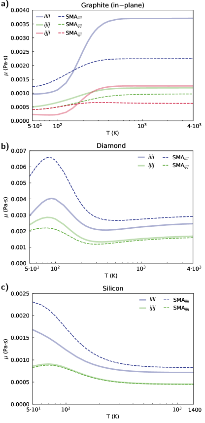
Figure 7: Comparison between the exact bulk thermal viscosity (solid lines) and the SMA bulk thermal viscosity (dashed line) for in-plane graphite (a), diamond (b) and silicon (c).

In this section we derive the expression for thermal viscosity within the single-mode relaxation-time approximation (SMA). Using the SMA, the LBTE at Eq. (40) becomes

$$\frac{\bm{v}_{\nu}}{\sqrt{\bar{N}_{\nu}(\bar{N}_{\nu}+1)}}\cdot\bigg{(}\frac{\partial N^{D}_{\nu}}{\partial\bm{u}}\cdot\nabla\bm{u}\bigg{)}=-\frac{\tilde{n}^{\delta{\rm E}}_{\nu}}{\tau^{\rm{}^{SMA}}_{\nu}}\;.$$ (50)

The deviation from equilibrium $\tilde{n}^{\delta{\rm E}}_{\nu}$ is readily found as

$$\tilde{n}^{\delta{\rm E}}_{\nu}=-\frac{\bm{v}_{\nu}}{\sqrt{\bar{N}_{\nu}(\bar{N}_{\nu}+1)}}\cdot\bigg{(}\frac{\partial N^{D}_{\nu}}{\partial\bm{u}}\cdot\nabla\bm{u}\bigg{)}\tau^{\rm{}^{SMA}}_{\nu}\;.$$ (51)

We insert this result in the definition of momentum flux, obtaining

$$\Pi^{ij}_{\delta\rm E,SMA} =\frac{1}{V}\sum_{\nu}{n}^{\delta{\rm E}}_{\nu}\hbar q^{i}{v}^{j}_{\nu}$$ (52)

$$=-\frac{1}{V}\sum_{\nu}\hbar^{2}q^{i}v^{j}_{\nu}{q}^{k}{v}^{l}_{\nu}\frac{\bar{N}_{\nu}\big{(}\bar{N}_{\nu}+1\big{)}}{k_{B}\bar{T}}\tau^{\rm{}^{SMA}}_{\nu}\frac{\partial u^{k}}{\partial r^{l}}\;.$$

From the definition of the thermal viscosity (8), the SMA thermal viscosity is therefore

$$\mu^{ijkl}_{\rm{\tiny SMA}}=\frac{\eta^{ijkl}_{\rm\tiny SMA}{+}\eta^{ilkj}_{\rm\tiny SMA}}{2}=\frac{1}{V}\sum_{\nu}\hbar^{2}q^{i}v^{j}_{\nu}{q}^{k}{v}^{l}_{\nu}\frac{\bar{N}_{\nu}\big{(}\bar{N}_{\nu}+1\big{)}}{k_{B}\bar{T}}\tau^{\rm{}^{SMA}}_{\nu}\;,$$ (53)

where we highlight the fact that in the SMA approximation $\eta^{ijkl}_{\rm SMA}=\mu^{ijkl}_{\rm SMA}$, since in the SMA the viscosity tensor $\eta^{ijkl}_{\rm SMA}$ has the $j{\leftrightarrow}l$ symmetry. A comparison between the exact bulk thermal viscosity (9) and the SMA bulk thermal viscosity (53) is shown in Fig. 7. We highlight how the SMA approximation — which neglects the off-diagonal elements of the scattering operator and works well when the Umklapp processes dominate over normal processes Guyer and Krumhansl (1966a); Fugallo et al. (2013); Lindsay (2016) — overestimates the largest component of the thermal viscosity, especially at low temperatures. This overestimation is more pronounced in diamond compared to silicon, in agreement with results from previous works where the SMA approximation was reported to yield quite accurate results for the thermal conductivity of silicon Cepellotti and Marzari (2016) but not for diamond Fugallo et al. (2013).

Appendix C Size effects on the thermal conductivity and viscosity

In order to obtain a simple estimate of size effects, we compute the total effective thermal conductivity and viscosity using a Matthiessen sum of the diffusive and ballistic limit:

$$\frac{1}{\kappa^{ij}} =\frac{1}{\kappa^{ij}_{\rm bulk}}{+}\frac{1}{\kappa^{ij}_{\rm ballistic}}\;,$$ (54)

$$\frac{1}{\mu^{ijkl}} =\frac{1}{\mu^{ijkl}_{\rm bulk}}{+}\frac{1}{\mu^{ijkl}_{\rm ballistic}}\;.$$ (55)

The ballistic conductivity and viscosity are computed for a sample of size $L_{S}$ as $\kappa^{ij}_{\rm ballistic}=K^{ij}_{S}\cdot L_{S}$ and $\mu^{ijkl}_{\rm ballistic}=M^{ijkl}\cdot L_{S}$, where the prefactors $K_{S}$ and $M^{ijkl}$ are

$$K^{ij}_{S} =\frac{1}{V}\sum_{\nu}(\hbar\omega_{\nu})^{2}\frac{\bar{N}_{\nu}(\bar{N}_{\nu}+1)}{k_{B}\bar{T}^{2}}v^{i}_{\nu}v^{j}_{\nu}\frac{1}{|\bm{v}_{\nu}|}\;,$$ (56)

$$M^{ijkl} =\frac{1}{V}\sum_{\nu}\hbar^{2}q^{i}v^{j}_{\nu}{q}^{k}{v}^{l}_{\nu}\frac{\bar{N}_{\nu}\big{(}\bar{N}_{\nu}+1\big{)}}{k_{B}\bar{T}}\frac{1}{|\bm{v}_{\nu}|}\;.$$ (57)

These prefactors are obtained after setting $\tau_{\nu}=\frac{L_{S}}{|\bm{v}_{\nu}|}$ in the SMA expressions of $k$ and $\mu$. $L_{S}$ is the length that determines boundary effects, i.e. the sample’s size for a single crystal or the grain size for a polycrystalline sample. The numerical values of $K^{ij}_{S}$ and $M^{ijkl}$ can be computed from first-principles and are tabulated in Tabs. 1, 2, 3.

Appendix D Viscous heat equations

In this section we derive an extension to Fourier’s law from the LBTE, which describes mesoscopic hydrodynamic thermal transport in terms of the temperature $T(\bm{r},t)$ and drift velocity $\bm{u}(\bm{r},t)$ fields. We focus on the mesoscopic regime where transport coefficients are well-defined and non-homogeneities arise from variations of the temperature and drift velocity. In contrast to Sec. II, here the temperature and drift velocity gradients are space-dependent, and consequently the LBTE is not linearized in the temperature and drift velocity gradients. We start recalling that hydrodynamic thermal transport emerges when most collisions between phonon wavepackets conserve the crystal momentum. This can happen, for example, when the mean free path for normal collisions $\Lambda^{N}$ is much smaller than the boundary scattering’s length $L_{S}$ (for a single crystal $L_{S}$ is the sample’s size, in the case of a polycrystalline sample $L_{S}$ is the size of the grains) or the mean free path for Umklapp collisions $\Lambda^{U}$: $\Lambda^{N}\ll L_{S},\Lambda^{U}$ Gurzhi (1968); Cepellotti et al. (2015). Under these conditions, the local equilibrium is expressed in terms of the four special eigenvectors $\phi^{0}_{\nu}$ (also denoted $\theta^{0}_{\nu}$, since this is a common eigenvector for the full and normal scattering operator, see Appendix A), $\phi^{i}_{\nu}$ ($i=1,2,3$) described in Sec. (A.1,A.2), and of the local temperature $T(\bm{r},t)$ and drift velocity $\bm{u}(\bm{r},t)$ fields. As explained in Sec. (A.1,A.2), these four special eigenvectors do not contribute to thermal conductivity and viscosity (i.e. they do not appear in Eqs. (6) and  (7)), since these latter coefficients only describe the response to a perturbation of the local equilibrium.

In order to exploit the relationship between the drift velocity $\bm{u}(\bm{r},t)$ and the drift eigenvectors $\phi^{i}_{\nu}$, we choose to work with the basis of eigenvectors of the normal scattering matrix $\tilde{\Omega}^{N}_{\nu{\nu^{\prime}}}$. To this aim, we diagonalize $\tilde{\Omega}^{N}_{\nu{\nu^{\prime}}}$ as

$$\frac{1}{V}\sum_{{\nu^{\prime}}}\tilde{\Omega}^{N}_{\nu{\nu^{\prime}}}\phi^{\beta}_{{\nu^{\prime}}}=\frac{1}{\tau^{N}_{\beta}}\phi^{\beta}_{\nu}\;,$$ (58)

where $\beta$ is an eigenvalue index, $\phi^{\beta}_{\nu}$ an eigenvector, and $\frac{1}{\tau^{N}_{\beta}}$ is an eigenvalue. Among these eigenvectors, we know the analytic expression for the 4 of them associated with energy and momentum conservation, which we label with $\beta=0$ for the energy eigenvector (in this section we will use $\phi^{0}_{\nu}$ to label the Bose-Einstein eigenvector (30)), and $\beta=1,\dots,3$ for the momentum eigenvectors, Eq. (34).

Noting that the set of “normal” eigenvectors $\{\phi^{\beta}_{\nu}\}$ (“normal” in the sense that they diagonalize $\tilde{\Omega}^{N}_{\nu{\nu^{\prime}}}$, the part of the scattering matrix that accounts for normal processes only) is a complete basis set Guyer and Krumhansl (1966a), we write the deviation from equilibrium $\tilde{n}_{\nu}(\bm{r},t)$ as a linear combination of these eigenvectors:

$$\tilde{n}_{\nu}(\bm{r},t)=\sum_{\beta}z_{\beta}(\bm{r},t)\phi_{\nu}^{\beta}\;.$$ (59)

After inserting Eq. (59) in (1), we write the LBTE in the basis of the eigenvectors of the normal scattering operator

$$\sum_{\beta} \frac{\partial z_{\beta}(\bm{r},t)}{\partial t}\phi_{\nu}^{\beta}+\bm{v}_{\nu}\cdot\bigg{(}\sum_{\beta}\nabla z_{\beta}(\bm{r},t)\phi_{\nu}^{\beta}\bigg{)}=$$

$$= -\sum_{\beta>3}\frac{z_{\beta}(\bm{r},t)}{\tau^{N}_{\beta}}\phi_{\nu}^{\beta}-\frac{1}{V}\sum_{{\nu^{\prime}},\beta>0}z_{\beta}(\bm{r},t)\tilde{\Omega}^{U}_{\nu{\nu^{\prime}}}\phi_{{\nu^{\prime}}}^{\beta}\;.$$ (60)

This equation is formally equivalent to the LBTE, but allows us to take advantage of the knowledge of the first $4$ eigenvectors to derive mesoscopic equations.

D.1 The projection of the LBTE on the $1^{\rm st}$ (Bose-Einstein) eigenvector: energy moment

Here we show how to obtain an energy balance equation. First, we note from Eq. (4) that the phonon population expansion of Eq. (59) can be recast as

$$\tilde{n}_{\nu} (\bm{r},t)=\tilde{n}^{T}_{\nu}(\bm{r},t)+\tilde{n}^{D}_{\nu}(\bm{r},t)+\tilde{n}^{\delta}_{\nu}(\bm{r},t)$$

$$= \sqrt{\frac{C}{k_{B}\bar{T}^{2}}}\phi^{0}_{\nu}(T(\bm{r},t)-\bar{T})+\sum_{i=1}^{3}\sqrt{\frac{A^{i}}{k_{B}\bar{T}}}\phi^{i}_{\nu}u^{i}(\bm{r},t)$$

$$+\sum_{\beta>3}\phi^{\beta}_{\nu}z_{\beta}(\bm{r},t)\;.$$ (61)

The coefficients $z_{\beta}$ in front of the $4$ special eigenvectors of $\tilde{\Omega}^{N}_{\nu{\nu^{\prime}}}$ are associated to temperature and drift velocity, which fully determine local equilibrium; in detail

$$z_{0}(\bm{r},t)=\sqrt{\frac{C}{k_{B}\bar{T}^{2}}}(T(\bm{r},t)-\bar{T})\;,$$ (62)

$$z_{i}(\bm{r},t)=\sqrt{\frac{A^{i}}{k_{B}\bar{T}}}u^{i}(\bm{r},t),\;i=1,2,3\;.$$ (63)

We now project the LBTE (60) in the subspace spanned by the Bose-Einstein eigenvector $\phi^{0}_{\nu}$, i.e. we take the scalar product of Eq. (60) with $\phi^{0}_{\nu}$, finding

$$\frac{\partial z_{0}(\bm{r},t)}{\partial t}+\sum_{\beta>0}\bm{W}_{0\beta}\cdot\nabla z_{\beta}(\bm{r},t)=0\;,$$ (64)

where we used the fact that $\phi^{0}_{\nu}$ is an eigenvector of zero eigenvalue to $\tilde{\Omega}^{U}_{\nu{\nu^{\prime}}}$ (see Sec. (A.1)) and we defined the velocity tensor

$$W^{j}_{\alpha\beta}=\frac{1}{V}\sum_{\nu}\phi_{\nu}^{\alpha}v^{j}_{\nu}\phi_{\nu}^{\beta}\;.$$ (65)

Note that the velocity $W^{j}_{\alpha\beta}$ differs from the velocity $w^{j}_{\alpha\beta}$ introduced in Sec. (II) for thermal viscosity; the difference arises from the use in Eq. (65) of the “normal” eigenvectors (of $\tilde{\Omega}^{N}_{\nu{\nu^{\prime}}}$) rather than the general eigenvectors of $\tilde{\Omega}_{\nu{\nu^{\prime}}}$ ($W^{j}_{\alpha\beta}\neq w^{j}_{\alpha\beta}$ in presence of Umklapp processes).

Substituting Eqs. (62, 63) in (64) we obtain

$$\sqrt{\frac{C}{k_{B}\bar{T}^{2}}}\frac{\partial T(\bm{r},t)}{\partial t} +\sum_{i,j=1}^{3}\sqrt{\frac{A^{i}}{k_{B}\bar{T}}}W_{0i}^{j}\frac{\partial u^{i}(\bm{r},t)}{\partial r^{j}}+$$

$$+\sum_{\beta>3}\bm{W}_{0\beta}\cdot\nabla z_{\beta}(\bm{r},t)=0\;.$$ (66)

To elucidate the meaning of this equation, we note that the harmonic heat flux can be written as Hardy (1963):

$$\bm{Q}(\bm{r},t) =\frac{1}{V}\sum_{\nu}\bm{v}_{\nu}\hbar\omega_{\nu}N_{\nu}(\bm{r},t)$$

$$=\frac{1}{V}\sum_{\nu}\bm{v}_{\nu}\hbar\omega_{\nu}\big{(}n^{D}_{\nu}(\bm{r},t)+n^{\delta{\rm O}}_{\nu}(\bm{r},t)\big{)}\;,$$ (67)

where we used the fact that only odd components of the phonon distribution contribute to the heat flux. Therefore, the heat flux receives contributions from both the drift velocity Simons (1983) and the temperature gradient Cepellotti and Marzari (2016). In the basis of “normal” eigenvectors, the drifting contribution can be written as

$$Q^{D,i}(\bm{r},t) =\frac{1}{V}\sum_{\nu}v^{i}_{\nu}\hbar\omega_{\nu}n^{D}_{\nu}(\bm{r},t)=$$

$$=\frac{1}{V}\sum_{\nu}v^{i}_{\nu}\hbar\omega_{\nu}\frac{\partial N^{D}_{\nu}}{\partial\bm{u}}\cdot\bm{u}(\bm{r},t)$$

$$=\frac{1}{V}\sum_{\nu,j}v^{i}_{\nu}\theta^{0}_{\nu}\sqrt{\bar{T}A^{j}C}\phi^{j}\bm{u}^{j}(\bm{r},t)$$

$$=\sum_{j}\sqrt{\bar{T}A^{j}C}W^{i}_{0j}\bm{u}^{j}(\bm{r},t)\;,$$ (68)

while for the contribution from the deviation from local equilibrium $n_{\nu}^{\delta{\rm O}}(\bm{r},t)$, we find

$$Q^{\delta{\rm O},i}(\bm{r},t) =\frac{1}{V}\sum_{\nu}{v}_{\nu}^{i}\hbar\omega_{\nu}n^{\delta{\rm O}}_{\nu}(\bm{r},t)$$

$$=\frac{1}{V}\sum_{\nu}{v}_{\nu}^{i}\hbar\omega_{\nu}\sqrt{\bar{N}_{\nu}(\bar{N}_{\nu}+1)}\tilde{n}^{\delta{\rm O}}_{\nu}(\bm{r},t)$$

$$=\frac{\sqrt{{Ck_{B}\bar{T}^{2}}}}{V}\sum_{\beta>3}\sum_{\nu}z_{\beta}(\bm{r},t)\phi^{0}_{\nu}v^{i}_{\nu}\phi_{\nu}^{\beta}$$

$$=\sqrt{Ck_{B}\bar{T}^{2}}\sum_{\beta>3}W^{i}_{0\beta}z_{\beta}(\bm{r},t)\;,$$ (69)

where only odd eigenvectors contribute ($W^{i}_{0\beta}=0$ for even $\beta$ eigenvectors). As explained in Sec. (A.3), the thermal conductivity is determined only from odd eigenvectors that are not related to local equilibrium (that is, all the odd eigenvectors minus the three drift eigenvectors). At this point it is crucial to recall that the relaxons have a well defined parity (even or odd), deriving from the symmetries of the full scattering operator $\tilde{\Omega}_{\nu{\nu^{\prime}}}=\tilde{\Omega}_{-\nu,-{\nu^{\prime}}}$ Hardy (1965, 1970). Because the same symmetries apply to $\tilde{\Omega}^{N}_{\nu,{\nu^{\prime}}}$, also the eigenvectors of the normal scattering operator have a well defined parity Hardy (1965, 1970); Hardy and Albers (1974). The odd component of the heat flux (and hence the thermal conductivity) is determined only from the odd part of the LBTE’s solution $\tilde{n}^{\delta{\rm O}}_{\nu}(\bm{r},t)$ Hardy (1965); Cepellotti and Marzari (2016), and this can be written either as a linear combination of odd relaxons (as done in Ref. Cepellotti and Marzari (2016)) or, equivalently, as a linear combination of odd eigenvectors of the normal scattering matrix, as done here. From the completeness of these basis sets it follows that the heat flux (69) arising from the odd out-of-equilibrium phonon distribution determined from equation (6), and described as a linear combination of odd eigenvectors of the normal scattering matrix, is equivalent to the heat flux of Ref. Cepellotti and Marzari (2016) that is written as a linear combination of odd relaxons (eigenvectors of the full scattering matrix). In an equivalent way, the equation for the odd part of the LBTE (6) is equivalent to the equation used to determine the thermal conductivity in Ref. Cepellotti and Marzari (2016), the only difference being the basis chosen for the decomposition of the solution (the relaxons in Ref. Cepellotti and Marzari (2016) and in the computation of the thermal viscosity reported in Fig. 1, and the eigenvectors of the normal scattering matrix here). The choice of the basis set does not affect the resulting local heat flux, which can therefore be related to the local temperature gradient via the thermal conductivity Cepellotti and Marzari (2016):

$$Q^{\delta{\rm O},i}(\bm{r},t)=-k^{ij}\nabla^{j}T(\bm{r},t)\;.$$ (70)

In Eq. (70) the thermal conductivity is space-independent, i.e. Eq. (70) is valid in the mesoscopic regime where the thermal conductivity and viscosity are space-independent and non-homogeneities arise solely from variations of the local temperature and local drift velocity. Eq. (70) can be used to rewrite Eq. (66) in terms of the local temperature and drift velocity fields, obtaining Eq. (10) of the main text:

$$C\frac{\partial T(\bm{r},t)}{\partial t} +\sum_{i,j=1}^{3}\sqrt{\bar{T}A^{i}C}W_{0i}^{j}\frac{\partial u^{i}(\bm{r},t)}{\partial r^{j}}$$

$$-\sum_{i,j=1}^{3}k^{ij}\frac{\partial^{2}T(\bm{r},t)}{\partial r^{i}\partial r^{j}}=0\;.$$ (71)

Eq. (71) is clearly not sufficient to fully describe the hydrodynamic heat conduction problem in which both $T(\bm{r},t)$ and $\bm{u}(\bm{r},t)$ are nonzero. In the next section we will derive a complementary set of equations that completes the formulation.

D.2 The projection of the LBTE on the $2^{\rm nd}/3^{\rm rd}/4^{\rm th}$ eigenvectors (the momentum eigenspace)

In this section, we derive a set of balance equations for crystal momentum. We start by recalling from Eq. (39) that the momentum flux receives contributions from three different terms. Of these three, the first term is a constant related to the equilibrium temperature, and thus is not changed by the LBTE. Therefore, we focus only on the momentum flux related to the local equilibrium temperature ${\Pi}^{ij}_{T}(\bm{r},t)$ and the out-of-equilibrium momentum flux generated in response to a drift velocity gradient ${\Pi}^{ij}_{\delta{\rm E}}(\bm{r},t)$. Using the expression of the four special eigenvectors discussed in Sec. (A.1, A.2), we rewrite these two momentum fluxes in the basis of eigenvectors of the normal scattering matrix, finding:

$$\Pi_{T}^{ij}(\bm{r},t) =\frac{1}{V}\sum_{\nu}\hbar q^{i}v^{j}n^{T}_{\nu}(\bm{r},t)$$

$$=\frac{1}{V}\sum_{\nu}\frac{\partial\bar{N}_{\nu}}{\partial T}\hbar q^{i}v^{j}(T(\mathbf{r},t)-\bar{T})$$

$$=\frac{1}{V}\sqrt{\frac{CA^{i}}{\bar{T}}}\sum_{\nu}\phi_{\nu}^{0}v^{j}\phi^{i}_{\nu}(T(\mathbf{r},t)-\bar{T})$$

$$=\sqrt{\frac{CA^{i}}{\bar{T}}}\sum_{i=3}^{3}W^{j}_{i0}(T(\mathbf{r},t)-\bar{T})\;,$$ (72)

and

$$\Pi_{\delta{\rm E}}^{ij}(\bm{r},t) =\frac{1}{V}\sum_{\nu}\hbar q^{i}v^{j}n^{\delta{\rm E}}_{\nu}n^{T}_{\nu}(\bm{r},t)$$

$$=\frac{\sqrt{k_{B}\bar{T}A^{i}}}{V}\sum_{\nu,\beta>3}\phi_{\nu}^{\beta}v^{j}_{\nu}\phi^{i}_{\nu}z_{\beta}(\bm{r},t)$$

$$=\sqrt{k_{B}\bar{T}A^{i}}\sum_{\beta>3}W^{j}_{i\beta}z_{\beta}(\bm{r},t)\;,$$ (73)

where we used the velocity tensor defined in Eq. (65).

Next, as in the previous section, we take the scalar product of Eq. (60) with $\phi^{i}_{\nu}\;(i=1,2,3)$, obtaining the following three equations indexed by $i=1,2,3$

$$\frac{\partial z_{i}(\bm{r},t)}{\partial t}+\bm{W}_{i0}\cdot\nabla z_{0}(\bm{r},t)+\sum_{\beta>3}\bm{W}_{i\beta}\cdot\nabla z_{\beta}(\bm{r},t)=$$

$$=-\sum_{j=1}^{3}z_{j}(\bm{r},t){D}_{U}^{ij}-\sum_{\beta>3}z_{\beta}(\bm{r},t){D}_{U}^{i\beta}\;,$$ (74)

where we used the fact that $\phi^{i}_{\nu}$ are eigenvectors of $\tilde{\Omega}^{N}_{\nu{\nu^{\prime}}}$ with zero eigenvalues and we defined

$${D}_{U}^{i\beta}=\frac{1}{V^{2}}\sum_{\nu,{\nu^{\prime}}}\phi_{\nu}^{i}\tilde{\Omega}^{U}_{\nu,{\nu^{\prime}}}\phi_{{\nu^{\prime}}}^{\beta}\;.$$ (75)

From the property $\tilde{\Omega}^{U}_{\nu,{\nu^{\prime}}}=\tilde{\Omega}^{U}_{-\nu,-{\nu^{\prime}}}$ it can be shown that ${D}_{U}^{i\beta}$ vanishes when $\beta$ indexes an even eigenvector. Since the coefficients $z_{\beta}(\bm{r},t)$ for the first four eigenvectors ($\beta=0,1,2,3$) are known, it is convenient to rewrite Eq. (74) as:

$$\frac{\partial z_{i}(\bm{r},t)}{\partial t}+\bm{W}_{i0}\cdot\nabla z_{0}(\bm{r},t)$$

$$+\sum_{\beta>3}\big{(}\bm{W}_{i\beta}\cdot\nabla+{D}_{U}^{i\beta}\big{)}z_{\beta}(\bm{r},t)=-\sum_{j=1}^{3}z_{j}(\bm{r},t){D}_{U}^{ij}\;,$$ (76)

In the hydrodynamic regime, Umklapp momentum dissipation is weak and thus ${D}_{U}^{i\beta}\to 0$ ($\phi^{i}_{\nu}$ is approximately an eigenvector with a vanishing eigenvalue for $\tilde{\Omega}^{U}_{\nu{\nu^{\prime}}}$). Therefore, we simplify Eq. (76) noting that

$$\sum_{\beta>3}\bm{W}_{i\beta}\cdot\nabla z_{\beta}(\bm{r},t)\gg\sum_{\beta>3}{D}_{U}^{i\beta}z_{\beta}(\bm{r},t)\;.$$ (77)

Then, we use the expression of the coefficients $z_{\beta}(\bm{r},t)$ ($\beta=0,1,2,3$), and substitute Eqs. (62,63) in the simplified Eq. (76), obtaining:

$$\sqrt{\frac{A^{i}}{k_{B}\bar{T}}}\frac{\partial u^{i}(\bm{r},t)}{\partial t}+\sqrt{\frac{C}{k_{B}\bar{T}^{2}}}\sum_{j=1}^{3}{W}_{i0}^{j}\frac{\partial T(\bm{r},t)}{\partial r^{j}}$$

$$+\frac{1}{\sqrt{k_{B}\bar{T}A^{i}}}\sum_{j}\frac{\partial{\Pi}^{ij}_{\delta{\rm E}}(\bm{r},t)}{\partial r^{j}}=-\sum_{j=1}^{3}\sqrt{\frac{A^{j}}{k_{B}\bar{T}}}{D}_{U}^{ij}u^{j}(\bm{r},t)\;.$$ (78)

Next, we note that only even eigenvectors different from the Bose-Einstein eigenvector determine the even distribution $n_{\nu}^{\delta{\rm E}}(\bm{r},t)$ appearing in the expression for the out-of-equilibrium momentum flux tensor (73). As shown in Eq. (47), in the mesoscopic regime the sum over the spatial derivatives of $\Pi_{\delta\rm{E}}^{ij}(\bm{r},t)$ can be expressed in terms of the viscosity and second derivative of the drift velocity. We thus find

$$A^{i}\frac{\partial u^{i}(\bm{r},t)}{\partial t}+\sqrt{\frac{CA^{i}}{\bar{T}}}\sum_{j=1}^{3}{W}_{i0}^{j}\frac{\partial T(\bm{r},t)}{\partial r^{j}}$$

$$-\sum_{j,k,l=1}^{3}\mu^{ijkl}\frac{\partial^{2}u^{k}(\bm{r},t)}{\partial r^{j}\partial r^{l}}=-\sum_{j=1}^{3}\sqrt{A^{i}A^{j}}{D}_{U}^{ij}u^{j}(\bm{r},t)\;.$$ (79)

Combining this with Eq. (71) we obtain $4$ equations to be solved in terms of temperature $T(\bm{r},t)$ and drift velocity $\bm{u}(\bm{r},t)$; these are the viscous heat equations at the core of this work and that are further discussed in the main text.

As a final remark it is worth mentioning that in the kinetic regime, characterized by strong crystal momentum dissipation, the inequality (77) may not be valid. Nevertheless, in such regime the strong crystal momentum dissipation ($\max_{ij}[D^{ij}_{U}]\to\infty$) yields the following (stronger) inequality

$$\frac{\partial z_{i}(\bm{r},t)}{\partial t}{+}\sum_{\beta>3}\big{(}\bm{W}_{i\beta}{\cdot}\nabla{+}{D}_{U}^{i\beta}\big{)}z_{\beta}(\bm{r},t)\ll-\sum_{j=1}^{3}z_{j}(\bm{r},t){D}_{U}^{ij},$$ (80)

implying that the viscous heat equations reduce to Fourier’s law, as discussed in Sec. VI.

From a mathematical point of view, the projection of the LBTE in the Bose-Einstein subspace, performed computing the scalar product between the LBTE in the normal eigenvectors basis (60) and the Bose-Einstein eigenvector (30) $\propto\omega_{\nu}$, is equivalent to calculating the energy moment of the LBTE. Analogously, the projection in the momentum subspace, performed calculating the scalar product between the LBTE (60) and the momentum eigenvectors (34) $\propto q^{i}$, is equivalent to computing the momentum moment of the LBTE.

Appendix E Parameters entering the viscous heat equations.

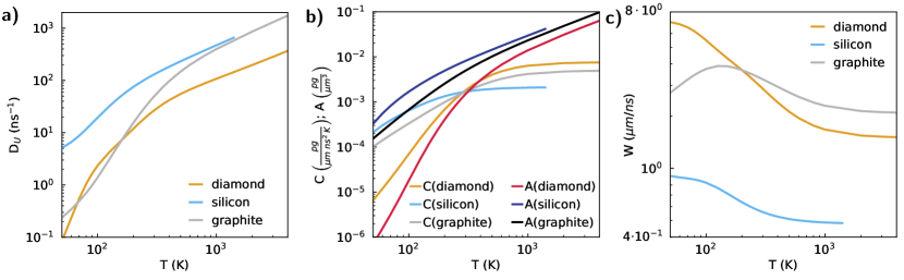
Figure 8: Trends as a function of the temperature of various quantities reported in Tabs. 1, 2, 3. Panel a), values of the momentum-dissipation inverse timescale $D_{U}(T)$; panel b), specific heat $C(T)$ and specific momentum $A(T)$; panel c), values of the velocity $W$.

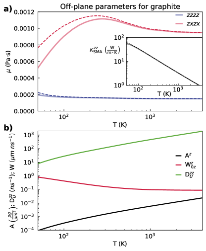
Figure 9: Panel a), off-plane thermal viscosity and off-plane SMA thermal conductivity (inset) of graphite for a sample having a grain size of 10 $\mu m$ (solid line) or for the bulk case (dashed line). The other components of the viscosity tensor involving off-plane directions are negligible (at least one order of magnitude smaller than the largest component reported here). Panel b), specific momentum $A^{z}$, component $W^{z}_{0z}$ of the velocity tensor, and component $D_{U}^{zz}$ of the momentum dissipation tensor of graphite.

We report in Fig. 8 the trends as a function of temperature of all the parameters needed to solve the viscous heat equations on the geometry of Fig. 3. Due to the crystal symmetries of the materials considered, several components of vectors and tensors are equivalent. 2^nd-rank tensors such as thermal conductivity ($\kappa^{ij}$), momentum dissipation (${D}_{U}^{ij}$) and velocity ($W^{j}_{0i}$) are isotropic and diagonal for diamond and silicon; for graphite they are isotropic and diagonal for in-plane ($x,y$) directions (as used in the geometry of Fig. 3). Similarly, the specific momentum $A^{i}$ is isotropic for diamond and silicon, and independent from the in-plane direction in graphite ($A^{x}=A^{y}$). The values of ${D}_{U}^{ij}$, $A^{i}$, $C$ and $W^{j}_{0i}$ as a function of temperature are plotted in Fig. 8 (we only report the in-plane or isotropic components, indexes are omitted). The numerical values of these parameters can be found in Tabs. 1, 2, 3; in addition, these tables contain also the prefactors discussed in Sec. II, III and Appendix C needed to compute the thermal conductivity in the ballistic limit $\kappa^{ij}_{\rm ballistic}$. In particular, the parameter $K^{ij}_{S}$ (defined for silicon, diamond and in-plane graphite), is defined as $K_{S}^{ij}=\kappa^{ij}_{\rm ballistic}/L_{S}$, where $L_{S}$ is the length that determines surface effects, i.e. the sample’s size for a single crystal or the grain size for a polycrystalline sample. In the tables, we also report the non-zero irreducible components of the bulk heat flux viscosity tensor, limiting graphite to in-plane components. The parameters $M^{ijkl}$ are the prefactors (defined in Appendix C) used to compute the ballistic thermal viscosity as $\mu^{ijkl}_{\rm ballistic}=M^{ijkl}\cdot L_{S}$. Similarly, the parameter $F_{U}^{ij}$ are defined as $F_{U}^{ij}={D}_{U,{\rm boundary}}^{ij}(L_{S})\cdot L_{S}$.

Additionally, Fig. 9 shows the off-plane transport coefficients (panel a) and the off-plane non-negligible values of $A^{i}$, ${D}_{U}^{ij}$, and $W^{j}_{0i}$ (panel b) for graphite; these parameters are not relevant for the geometry studied in Sec. V and are reported for completeness.

Table 1: Parameters entering the viscous heat equations for graphite. We report here only the in-plane components of the tensors needed to perform the calculation of Fig. 3: $\kappa^{ij}_{\rm P}=\kappa_{\rm P}\delta^{ij}$, $\kappa^{ij}_{\rm C}=\kappa_{\rm C}\delta^{ij}$, $K^{ij}_{S}=K_{S}\delta^{ij}$, ${D}_{U}^{ij}={D}_{U}\delta^{ij}$, ${F}_{U}^{ij}={F}_{U}\delta^{ij}$, $A=A^{i}\;\forall\;i$, $W^{j}_{0i}=W^{j}_{i0}=W\delta^{ij}$, where the indexes $i,j$ represent the in-plane directions $x,y$ only ($i,j=1,2$).

T [K]	$\kappa_{\rm P}\;\big{[}\rm\frac{W}{m{\cdot}K}\big{]}$	$\kappa_{\rm C}\;\big{[}\rm\frac{W}{m{\cdot}K}\big{]}$	${K_{S}\;\big{[}\rm\frac{W}{m^{2}{\cdot}K}\big{]}}$	$\mu^{iiii}\;[\rm Pa{\cdot}s]$	$\mu^{ijij}\;[\rm Pa{\cdot}s]$	$\mu^{iijj}\;[\rm Pa{\cdot}s]$	$M^{iiii}\;[\rm\frac{Pa{\cdot}s}{m}]$	$M^{ijij}\;[\rm\frac{Pa{\cdot}s}{m}]$	$M^{ijji}\;[\rm\frac{Pa{\cdot}s}{m}]$	${D}_{U}\;[\rm ns^{-1}]$	${F}_{U}\;[\rm\frac{m}{s}]$	A $\big{[}\rm\frac{pg}{\mu m^{3}}\big{]}$	$C$ $\big{[}\rm\frac{pg}{\mu m{\cdot}ns^{2}{\cdot}K}\big{]}$	W $\big{[}\rm\frac{\mu m}{ns}\big{]}$
50	4.05937e+03	1.68603e-04	2.57075e+08	9.64173e-04	5.02673e-04	2.28503e-04	4.39176e+02	1.46638e+02	1.46269e+02	2.35602e-01	4.26877e+03	1.53433e-04	1.00900e-04	2.72761e+00
60	4.71660e+03	2.57901e-04	3.95197e+08	9.71961e-04	5.28685e-04	2.19176e-04	7.15578e+02	2.39244e+02	2.38166e+02	3.43827e-01	4.59801e+03	2.29498e-04	1.41101e-04	3.00647e+00
70	5.30227e+03	3.86737e-04	5.59073e+08	9.91550e-04	5.60889e-04	2.12711e-04	1.07264e+03	3.59308e+02	3.56660e+02	4.90888e-01	4.88642e+03	3.20256e-04	1.84524e-04	3.25249e+00
80	5.73508e+03	5.99494e-04	7.45726e+08	1.02183e-03	5.95233e-04	2.10580e-04	1.51011e+03	5.07190e+02	5.01440e+02	6.99024e-01	5.13608e+03	4.25102e-04	2.30997e-04	3.45924e+00
85	5.88316e+03	7.64389e-04	8.46709e+08	1.04140e-03	6.12652e-04	2.11623e-04	1.75824e+03	5.91502e+02	5.83334e+02	8.33461e-01	5.24694e+03	4.82650e-04	2.55380e-04	3.54681e+00
90	5.98509e+03	9.89803e-04	9.52360e+08	1.06450e-03	6.30069e-04	2.14443e-04	2.02532e+03	6.82640e+02	6.71286e+02	9.92275e-01	5.34894e+03	5.43532e-04	2.80534e-04	3.62371e+00
100	6.05968e+03	1.70592e-03	1.17648e+09	1.12368e-03	6.64594e-04	2.26760e-04	2.61392e+03	8.85020e+02	8.64331e+02	1.39551e+00	5.52812e+03	6.75030e-04	3.33160e-04	3.74625e+00
125	5.68808e+03	6.19470e-03	1.79932e+09	1.36901e-03	7.47169e-04	3.08284e-04	4.37038e+03	1.50275e+03	1.43336e+03	3.03975e+00	5.85614e+03	1.05685e-03	4.77779e-04	3.89427e+00
150	4.95001e+03	1.68525e-02	2.48830e+09	1.74338e-03	8.22466e-04	4.58198e-04	6.46259e+03	2.26630e+03	2.09701e+03	5.82976e+00	6.06477e+03	1.50504e-03	6.38359e-04	3.88637e+00
175	4.19048e+03	3.54534e-02	3.21691e+09	2.16305e-03	8.89217e-04	6.35206e-04	8.81058e+03	3.15609e+03	2.82509e+03	9.95230e+00	6.20314e+03	2.00676e-03	8.09822e-04	3.80167e+00
200	3.53715e+03	6.22028e-02	3.96223e+09	2.54485e-03	9.46684e-04	7.98006e-04	1.13505e+04	4.15136e+03	3.59604e+03	1.54740e+01	6.30063e+03	2.54990e-03	9.86974e-04	3.68920e+00
225	3.00949e+03	9.60903e-02	4.70645e+09	2.85177e-03	9.94791e-04	9.28042e-04	1.40336e+04	5.23216e+03	4.39558e+03	2.23622e+01	6.37337e+03	3.12432e-03	1.16581e-03	3.57259e+00
250	2.59110e+03	1.35378e-01	5.43687e+09	3.08241e-03	1.03413e-03	1.02427e-03	1.68237e+04	6.38073e+03	5.21448e+03	3.05105e+01	6.43012e+03	3.72211e-03	1.34366e-03	3.46122e+00
275	2.25923e+03	1.78035e-01	6.14489e+09	3.25018e-03	1.06572e-03	1.09285e-03	1.96938e+04	7.58209e+03	6.04680e+03	3.97658e+01	6.47577e+03	4.33732e-03	1.51881e-03	3.35792e+00
300	1.99378e+03	2.22075e-01	6.82487e+09	3.37078e-03	1.09079e-03	1.14103e-03	2.26238e+04	8.82402e+03	6.88860e+03	4.99551e+01	6.51324e+03	4.96554e-03	1.69010e-03	3.26300e+00
350	1.60318e+03	3.07855e-01	8.08784e+09	3.52011e-03	1.12596e-03	1.19869e-03	2.86057e+04	1.13924e+04	8.59058e+03	7.24549e+01	6.57048e+03	6.24865e-03	2.01775e-03	3.09612e+00
400	1.33509e+03	3.83750e-01	9.21271e+09	3.59939e-03	1.14751e-03	1.22790e-03	3.46848e+04	1.40297e+04	1.03064e+04	9.68155e+01	6.61114e+03	7.55350e-03	2.32135e-03	2.95575e+00
500	9.98702e+02	4.95975e-01	1.10594e+10	3.66770e-03	1.16905e-03	1.25159e-03	4.69490e+04	1.93852e+04	1.37502e+04	1.47964e+02	6.66215e+03	1.01896e-02	2.84581e-03	2.73866e+00
600	7.99431e+02	5.63451e-01	1.24444e+10	3.69035e-03	1.17775e-03	1.25863e-03	5.92022e+04	2.47475e+04	1.71850e+04	1.99654e+02	6.69043e+03	1.28283e-02	3.26054e-03	2.58552e+00
800	5.75423e+02	6.24987e-01	1.42502e+10	3.70056e-03	1.18356e-03	1.26080e-03	8.34395e+04	3.53375e+04	2.39875e+04	3.00624e+02	6.71747e+03	1.80581e-02	3.82784e-03	2.39757e+00
1000	4.52004e+02	6.47048e-01	1.52910e+10	3.70106e-03	1.18535e-03	1.26010e-03	1.07299e+05	4.57299e+04	3.07007e+04	3.97914e+02	6.72894e+03	2.32138e-02	4.16766e-03	2.29514e+00
2000	2.21503e+02	6.74660e-01	1.69581e+10	3.70084e-03	1.18829e-03	1.25838e-03	2.23610e+05	9.61271e+04	6.35592e+04	8.57330e+02	6.74228e+03	4.83715e-02	4.73019e-03	2.13973e+00
3000	1.47397e+02	6.92956e-01	1.73097e+10	3.70278e-03	1.18973e-03	1.25860e-03	3.38143e+05	1.45600e+05	9.59938e+04	1.30189e+03	6.74440e+03	7.31498e-02	4.85155e-03	2.10827e+00
4000	1.10542e+02	7.11733e-01	1.74364e+10	3.70441e-03	1.19062e-03	1.25896e-03	4.52156e+05	1.94803e+05	1.28304e+05	1.74234e+03	6.74511e+03	9.78154e-02	4.89550e-03	2.09705e+00

Table 2: Parameters entering the viscous heat equations for diamond. As discussed above, due to the symmetries of diamond’s crystal, $\kappa^{ij}_{\rm P}=\kappa_{\rm P}\delta^{ij}$, $\kappa^{ij}_{\rm C}=\kappa_{\rm C}\delta^{ij}$, $K^{ij}_{S}=K_{S}\delta^{ij}$, ${D}_{U}^{ij}={D}_{U}\delta^{ij}$, ${F}_{U}^{ij}={F}_{U}\delta^{ij}$, $A=A^{i}\;\forall\;i$, $W^{j}_{0i}=W^{j}_{i0}=W\delta^{ij}$, where $i,j=1,{\cdots},3$.

T [K]	$\kappa_{\rm P}\;\big{[}\rm\frac{W}{m{\cdot}K}\big{]}$	$\kappa_{\rm C}\;\big{[}\rm\frac{W}{m{\cdot}K}\big{]}$	${K_{S}\;\big{[}\rm\frac{W}{m^{2}{\cdot}K}\big{]}}$	$\mu^{iiii}\;[\rm Pa{\cdot}s]$	$\mu^{ijij}\;[\rm Pa{\cdot}s]$	$M^{iiii}\;[\rm\frac{Pa{\cdot}s}{m}]$	$M^{ijij}\;[\rm\frac{Pa{\cdot}s}{m}]$	${D}_{U}\;[\rm ns^{-1}]$	${F}_{U}\;[\rm\frac{m}{s}]$	A $\big{[}\rm\frac{pg}{\mu m^{3}}\big{]}$	$C$ $\big{[}\rm\frac{pg}{\mu m{\cdot}ns^{2}{\cdot}K}\big{]}$	W $\big{[}\rm\frac{\mu m}{ns}\big{]}$
50	3.43111e+04	2.07528e-05	2.73909e+07	2.95594e-03	2.39102e-03	5.06687e+00	1.68663e+00	8.37822e-02	1.20887e+04	6.98185e-07	6.53393e-06	6.98908e+00
60	3.28294e+04	4.82483e-05	4.87721e+07	3.42258e-03	2.65063e-03	1.10924e+01	3.61332e+00	2.36470e-01	1.17603e+04	1.55771e-06	1.18825e-05	6.79196e+00
70	3.05315e+04	9.23559e-05	7.95828e+07	3.77282e-03	2.80007e-03	2.16728e+01	7.01404e+00	5.51176e-01	1.13049e+04	3.15801e-06	1.99510e-05	6.51375e+00
80	2.77912e+04	1.57229e-04	1.22126e+08	3.97491e-03	2.85772e-03	3.90900e+01	1.27110e+01	1.04179e+00	1.07756e+04	5.98689e-06	3.16787e-05	6.17705e+00
90	2.48308e+04	2.52625e-04	1.78772e+08	4.03466e-03	2.83659e-03	6.62241e+01	2.18227e+01	1.66305e+00	1.02476e+04	1.07215e-05	4.80997e-05	5.82219e+00
100	2.18775e+04	3.96722e-04	2.51659e+08	3.98459e-03	2.75499e-03	1.06364e+02	3.57240e+01	2.35506e+00	9.77500e+03	1.81905e-05	7.02007e-05	5.48421e+00
125	1.54475e+04	1.17600e-03	5.13987e+08	3.60462e-03	2.41425e-03	2.85397e+02	1.01522e+02	4.21125e+00	8.92029e+03	5.47561e-05	1.55097e-04	4.80253e+00
150	1.08162e+04	3.12615e-03	8.93341e+08	3.14294e-03	2.05193e-03	6.09964e+02	2.29408e+02	6.31694e+00	8.41644e+03	1.26987e-04	2.86510e-04	4.32960e+00
175	7.74443e+03	7.08919e-03	1.37511e+09	2.76384e-03	1.77050e-03	1.10184e+03	4.34626e+02	8.87028e+00	8.09518e+03	2.43489e-04	4.63817e-04	3.97834e+00
200	5.78523e+03	1.38027e-02	1.93367e+09	2.49842e-03	1.58204e-03	1.76124e+03	7.22624e+02	1.19199e+01	7.86336e+03	4.07776e-04	6.82343e-04	3.69265e+00
225	4.53806e+03	2.36643e-02	2.54139e+09	2.32532e-03	1.46502e-03	2.57437e+03	1.09085e+03	1.53786e+01	7.67879e+03	6.19378e-04	9.35200e-04	3.44745e+00
250	3.72328e+03	3.66215e-02	3.17342e+09	2.21560e-03	1.39570e-03	3.52071e+03	1.53178e+03	1.91087e+01	7.52304e+03	8.75213e-04	1.21427e-03	3.23270e+00
275	3.16907e+03	5.21840e-02	3.80954e+09	2.14710e-03	1.35666e-03	4.57803e+03	2.03552e+03	2.29796e+01	7.38778e+03	1.17073e-03	1.51104e-03	3.04395e+00
300	2.77499e+03	6.95343e-02	4.43449e+09	2.10528e-03	1.33661e-03	5.72518e+03	2.59170e+03	2.68886e+01	7.26885e+03	1.50073e-03	1.81740e-03	2.87843e+00
350	2.25727e+03	1.05819e-01	5.61142e+09	2.06829e-03	1.32779e-03	8.21663e+03	3.82299e+03	3.45670e+01	7.07083e+03	2.24339e-03	2.43160e-03	2.60738e+00
400	1.93101e+03	1.39434e-01	6.65793e+09	2.06410e-03	1.33876e-03	1.08779e+04	5.16074e+03	4.18582e+01	6.91554e+03	3.06547e-03	3.01541e-03	2.40095e+00
500	1.53218e+03	1.92815e-01	8.33667e+09	2.09261e-03	1.37770e-03	1.64273e+04	7.98902e+03	5.51336e+01	6.69637e+03	4.83923e-03	4.01807e-03	2.12089e+00
600	1.28760e+03	2.33780e-01	9.54694e+09	2.13344e-03	1.41760e-03	2.20429e+04	1.08752e+04	6.69946e+01	6.55639e+03	6.67950e-03	4.78618e-03	1.94940e+00
800	9.89166e+02	2.97535e-01	1.10517e+10	2.20690e-03	1.48108e-03	3.30993e+04	1.65761e+04	8.81536e+01	6.39925e+03	1.03530e-02	5.78811e-03	1.76384e+00
1000	8.07834e+02	3.45553e-01	1.18801e+10	2.26142e-03	1.52541e-03	4.38462e+04	2.21156e+04	1.07517e+02	6.31958e+03	1.39372e-02	6.35996e-03	1.67254e+00
2000	4.26034e+02	4.74596e-01	1.31490e+10	2.38976e-03	1.62563e-03	9.50713e+04	4.84227e+04	1.96731e+02	6.20573e+03	3.09257e-02	7.26149e-03	1.54525e+00
3000	2.90112e+02	5.43241e-01	1.34078e+10	2.43788e-03	1.66217e-03	1.44824e+05	7.38984e+04	2.83004e+02	6.18362e+03	4.73219e-02	7.44892e-03	1.52096e+00
4000	2.20060e+02	5.95281e-01	1.35003e+10	2.46306e-03	1.68105e-03	1.94151e+05	9.91319e+04	3.68665e+02	6.17580e+03	6.35407e-02	7.51621e-03	1.51241e+00

Table 3: Parameters entering the viscous heat equations for silicon. As discussed above, due to the symmetries of silicon’s crystal, $\kappa^{ij}_{\rm P}=\kappa_{\rm P}\delta^{ij}$, $\kappa^{ij}_{\rm C}=\kappa_{\rm C}\delta^{ij}$, $K^{ij}_{S}=K_{S}\delta^{ij}$, ${D}_{U}^{ij}={D}_{U}\delta^{ij}$, ${F}_{U}^{ij}={F}_{U}\delta^{ij}$, $A=A^{i}\;\forall\;i$, $W^{j}_{0i}=W^{j}_{i0}=W\delta^{ij}$, where $i,j=1,{\cdots},3$.

T [K]	$\kappa_{\rm P}\;\big{[}\rm\frac{W}{m{\cdot}K}\big{]}$	$\kappa_{\rm C}\;\big{[}\rm\frac{W}{m{\cdot}K}\big{]}$	${K_{S}\;\big{[}\rm\frac{W}{m^{2}{\cdot}K}\big{]}}$	$\mu^{iiii}\;[\rm Pa{\cdot}s]$	$\mu^{ijij}\;[\rm Pa{\cdot}s]$	$M^{iiii}\;[\rm\frac{Pa{\cdot}s}{m}]$	$M^{ijij}\;[\rm\frac{Pa{\cdot}s}{m}]$	${D}_{U}\;[\rm ns^{-1}]$	${F}_{U}\;[\rm\frac{m}{s}]$	A $\big{[}\rm\frac{pg}{\mu m^{3}}\big{]}$	$C$ $\big{[}\rm\frac{pg}{\mu m{\cdot}ns^{2}{\cdot}K}\big{]}$	W $\big{[}\rm\frac{\mu m}{ns}\big{]}$
50	2.23795e+03	4.59329e-02	2.20201e+08	1.68379e-03	8.58240e-04	3.33315e+02	2.76288e+02	5.11570e+00	2.70364e+03	3.27665e-04	2.11441e-04	9.02735e-01
60	1.81398e+03	7.09541e-02	3.15143e+08	1.58868e-03	8.96618e-04	5.52469e+02	4.76459e+02	6.62366e+00	2.71505e+03	5.54460e-04	3.02489e-04	8.85284e-01
70	1.47266e+03	9.57185e-02	4.08143e+08	1.49577e-03	9.08048e-04	8.04123e+02	7.07599e+02	8.78307e+00	2.72606e+03	8.14113e-04	3.91395e-04	8.73874e-01
80	1.19453e+03	1.18329e-01	4.97327e+08	1.40019e-03	8.93142e-04	1.07864e+03	9.57983e+02	1.16582e+01	2.73491e+03	1.09495e-03	4.77916e-04	8.61085e-01
90	9.74026e+02	1.37274e-01	5.82183e+08	1.30833e-03	8.61466e-04	1.36970e+03	1.22015e+03	1.52308e+01	2.74122e+03	1.38989e-03	5.62856e-04	8.44738e-01
100	8.03719e+02	1.51720e-01	6.62519e+08	1.22579e-03	8.22564e-04	1.67298e+03	1.48947e+03	1.94247e+01	2.74509e+03	1.69464e-03	6.46690e-04	8.25091e-01
125	5.32796e+02	1.69276e-01	8.42648e+08	1.06829e-03	7.27720e-04	2.46564e+03	2.17760e+03	3.19146e+01	2.74649e+03	2.48348e-03	8.49829e-04	7.69340e-01
150	3.87535e+02	1.70507e-01	9.92662e+08	9.66838e-04	6.55421e-04	3.28405e+03	2.87136e+03	4.60065e+01	2.74093e+03	3.29333e-03	1.03633e-03	7.16183e-01
175	3.02197e+02	1.66898e-01	1.11455e+09	9.00619e-04	6.04637e-04	4.11081e+03	3.56215e+03	6.06265e+01	2.73283e+03	4.11117e-03	1.19918e-03	6.71955e-01
200	2.47534e+02	1.63344e-01	1.21236e+09	8.55850e-04	5.69080e-04	4.93707e+03	4.24698e+03	7.52349e+01	2.72447e+03	4.92977e-03	1.33675e-03	6.36972e-01
225	2.09966e+02	1.60900e-01	1.29062e+09	8.24499e-04	5.43728e-04	5.75879e+03	4.92514e+03	8.96094e+01	2.71681e+03	5.74536e-03	1.45094e-03	6.09681e-01
250	1.82675e+02	1.59448e-01	1.35343e+09	8.01853e-04	5.25234e-04	6.57443e+03	5.59687e+03	1.03682e+02	2.71013e+03	6.55621e-03	1.54510e-03	5.88350e-01
275	1.61970e+02	1.58683e-01	1.40415e+09	7.85055e-04	5.11434e-04	7.38370e+03	6.26280e+03	1.17454e+02	2.70443e+03	7.36173e-03	1.62269e-03	5.71533e-01
300	1.45710e+02	1.58355e-01	1.44545e+09	7.72310e-04	5.00922e-04	8.18690e+03	6.92362e+03	1.30950e+02	2.69961e+03	8.16196e-03	1.68684e-03	5.58128e-01
350	1.21755e+02	1.58409e-01	1.50744e+09	7.54699e-04	4.86338e-04	9.77722e+03	8.23261e+03	1.57251e+02	2.69211e+03	9.74789e-03	1.78475e-03	5.38497e-01
400	1.04880e+02	1.58914e-01	1.55067e+09	7.43511e-04	4.77032e-04	1.13499e+04	9.52838e+03	1.82836e+02	2.68671e+03	1.13174e-02	1.85414e-03	5.25164e-01
500	8.25113e+01	1.60439e-01	1.60486e+09	7.30895e-04	4.66472e-04	1.44577e+04	1.20928e+04	2.32571e+02	2.67977e+03	1.44204e-02	1.94232e-03	5.08869e-01
600	6.82316e+01	1.62305e-01	1.63594e+09	7.24532e-04	4.61092e-04	1.75321e+04	1.46339e+04	2.81113e+02	2.67571e+03	1.74906e-02	1.99348e-03	4.99732e-01
800	5.08841e+01	1.66661e-01	1.66806e+09	7.18968e-04	4.56298e-04	2.36251e+04	1.96779e+04	3.76331e+02	2.67145e+03	2.35755e-02	2.04682e-03	4.90446e-01
1000	4.06552e+01	1.71502e-01	1.68337e+09	7.16939e-04	4.54479e-04	2.96784e+04	2.46951e+04	4.70285e+02	2.66941e+03	2.96202e-02	2.07239e-03	4.86079e-01
1200	3.38805e+01	1.76561e-01	1.69180e+09	7.16146e-04	4.53716e-04	3.57109e+04	2.96982e+04	5.63606e+02	2.66828e+03	3.56437e-02	2.08651e-03	4.83688e-01
1400	2.90538e+01	1.81710e-01	1.69692e+09	7.15858e-04	4.53394e-04	4.17311e+04	3.46933e+04	6.56567e+02	2.66759e+03	4.16548e-02	2.09512e-03	4.82240e-01

Appendix F Second sound

In this section we show that drifting second sound Guyer and Krumhansl (1966b); Hardy (1970); Cepellotti and Marzari (2017b); Huberman et al. (2019), i.e. thermal transport in terms of a temperature damped wave, is described by the viscous heat equations. We will first show the emergence of second sound following a bottom-up approach, i.e. analyzing the conditions under which the two viscous heat equations decouple with the first equation (10) reducing to a damped wave equations for the temperature field. Afterwards, we will analyze second sound within the viscous heat equations following a top-down approach, i.e. requiring the temperature field to have the mathematical form of a damped wave and analyzing if and under which conditions this can emerge from the viscous heat equations.

F.1 Second sound from the viscous heat equations (bottom-up approach)

For simplicity, we consider a system such that the tensors $W^{i}_{0j}$ and $\kappa^{ij}$ appearing in the viscous heat equations (10,11) are isotropic; the generalization to an anisotropic case is analogous to what is reported here.

Without loss of generality, we consider $\hat{x}$ as the direction of second sound propagation. For simplicity we consider an isotropic system; the general derivation can be obtained straightforwardly generalizing the procedure reported here. In an isotropic system, the drifting heat flux $\bm{Q}^{D}(\bm{r},t)$ is collinear with the drift velocity and the heat flux due to local temperature changes $\bm{Q}^{\delta}(\bm{r},t)$ is collinear with the temperature gradient. Thus, it follows that the only nonzero component of the drift velocity must be along the second sound propagation direction $u^{x}=u$ (for simplicity we omit all tensor indexes in the rest of this section, since the only the component having all the indexes equal to $x$ is needed for this discussion). With these conditions, the viscous heat equations (10,11) become:

$$C\frac{\partial T(x,t)}{\partial t}+W\sqrt{\bar{T}AC}\frac{\partial u(x,t)}{\partial x}-\kappa\frac{\partial^{2}T(x,t)}{\partial x^{2}}=0\;,$$ (81)

$$\begin{split}A\frac{\partial u(x,t)}{\partial t}+\sqrt{\frac{CA}{\bar{T}}}{W}\frac{\partial T(x,t)}{\partial x}&-\mu\frac{\partial^{2}u(x,t)}{\partial x^{2}}\\ &=-A\;{D}_{U}u(x,t)\;.\end{split}$$ (82)

In order to observe second sound, temperature changes need to propagate following a damped wave equation. To this aim, we require that drift velocity and temperature are related as

$$W\sqrt{\bar{T}AC}\frac{\partial u(x,t)}{\partial x}=C\tau_{ss}(1-f)\frac{\partial^{2}T(x,t)}{\partial t^{2}}-Cf\frac{\partial T(x,t)}{\partial t}\;.$$ (83)

where $\tau_{ss}$ is the second sound relaxation time and $0{<}|f|{<}1$ is a constant, both to be determined. To better understand this requirement, we insert Eq. (83) in Eq. (81), finding the desired temperature damped-wave equation:

$$\frac{\partial^{2}T(x,t)}{\partial t^{2}}+\frac{1}{\tau_{ss}}\frac{\partial T(x,t)}{\partial t}-\frac{\kappa}{C\tau_{ss}(1-f)}\frac{\partial^{2}T(x,t)}{\partial x^{2}}=0\;.$$ (84)

Next, we show that condition (83) implies that also the drift velocity field follows a damped-wave equation. To this aim, we take the derivative with respect to $x$ of Eq. (83), finding

$$W\sqrt{\bar{T}AC}\frac{\partial^{2}u(x,t)}{\partial^{2}x}=\underbrace{\left(C\tau_{ss}(1-f)\frac{\partial^{2}}{\partial t^{2}}-Cf\frac{\partial}{\partial t}\right)}_{\hat{O}}\frac{\partial T(x,t)}{\partial x}\;,$$ (85)

where $\hat{O}$ is a differential operator. Next, by applying the operator $\hat{O}$ to both sides of equation (82) and using condition (85), we obtain

$$\begin{split}\frac{\partial^{3}u(x,t)}{\partial t^{3}}&-\frac{f}{1-f}\frac{1}{\tau_{ss}}\frac{\partial^{2}u(x,t)}{\partial t^{2}}+\frac{{W}^{2}}{\tau_{ss}(1-f)}\frac{\partial^{2}u(x,t)}{\partial x^{2}}\\ &-\frac{\mu}{A}\frac{\partial^{4}u(x,t)}{\partial t^{2}\partial x^{2}}+\frac{f}{1-f}\frac{1}{\tau_{ss}}\frac{\mu}{A}\frac{\partial^{3}u(x,t)}{\partial t\partial x^{2}}\\ &=-{D}_{U}\left(\frac{\partial^{2}u(x,t)}{\partial t^{2}}-\frac{f}{1-f}\frac{1}{\tau_{ss}}\frac{\partial u(x,t)}{\partial t}\right)\;.\end{split}$$ (86)

If we consider only the lowest-order derivatives in Eq. (86), we obtain a simplified equation that holds in the close-to-equilibrium regime where variations in space and time are small. In particular, neglecting higher-than-second order derivatives gives:

$$\begin{split}\frac{\partial^{2}u(x,t)}{\partial t^{2}}&+\underbrace{\frac{{D}_{U}f}{f{-}(1{-}f)\tau_{ss}{D}_{U}}}_{c_{1}}\frac{\partial u(x,t)}{\partial t}\\ &-\underbrace{\frac{W^{2}}{f{-}(1{-}f)\tau_{ss}{D}_{U}}}_{c_{2}}\frac{\partial^{2}u(x,t)}{\partial x^{2}}=0\;.\end{split}$$ (87)

Therefore, if

$$f>\frac{\tau_{ss}{D}_{U}}{1+\tau_{ss}{D}_{U}}\;,$$ (88)

then both constants $c_{1}$ and $c_{2}$ are positive and the evolution of the drift velocity is that of a damped wave equation like the one for temperature.

The coefficients $\tau_{ss}$ and $f$ are determined solving Eqs. (84,87) and imposing the second sound condition (83). The solutions are of the form

$$T(x,t)=\frac{1}{2\pi}\int C_{T}(k)e^{-\frac{t}{2\tau_{ss}}}e^{i(kx-\bar{\omega}(k)t)}dk$$ (89)

and

$$u(x,t)=\frac{1}{2\pi}\int C_{u}(k)e^{-\frac{t}{2\tau_{ss}}}e^{i(kx-\bar{\omega}(k)t)}dk$$ (90)

with:

$$\bar{\omega}(k)=\sqrt{v_{ss}^{2}k^{2}-\frac{1}{4\tau^{2}_{ss}}}\;;$$ (91)

$$v_{g}(k)=\frac{\partial\bar{\omega}(k)}{\partial k}=\frac{kv_{ss}}{\sqrt{k^{2}+(2\tau_{ss}v_{ss})^{-2}}}\;;$$ (92)

$$f={D}_{U}\tau_{ss}\;;$$ (93)

$$\tau_{ss}=\frac{C({W})^{2}}{\kappa({D}_{U})^{2}+{D}_{U}C({W})^{2}}\;;$$ (94)

$$v_{ss}=\frac{\kappa{D}_{U}+C{W}^{2}}{C{W}}\;.$$ (95)

The condition (93) is derived from the requirement $c_{1}=\frac{1}{\tau_{ss}}$, and is consistent with the damped wave requirement (88); condition (94) is derived from the requirement that $c_{2}=\frac{\kappa}{C\tau_{ss}(1-f)}$ and the second sound velocity (95) has been obtained substituting Eq. (93) and Eq. (94) into Eq. (84). We note that for ${D}_{U}\to 0$ (that is, negligible crystal momentum dissipation) $v_{g}(k)\to v_{ss}\to{W}$, i.e. the second sound propagation velocity approaches the drifting second sound velocity defined by Hardy Hardy (1970)) and $\tau_{ss}\to{D_{U}}^{-1}$. Finally, the second sound condition (83) imposes the following relation between the coefficients:

$$\begin{split}C_{u}(k)&{=}\frac{-i}{k}\bigg{\{}\frac{\tau_{ss}}{{W}}\sqrt{\frac{C}{\bar{T}A}}\bigg{[}(1-\tau_{ss}{D}_{U})\left(\frac{1}{2\tau_{ss}}{+}i\bar{\omega}(k)\right)^{2}\\ &+{D}_{U}\left(\frac{1}{2\tau_{ss}}{+}i\bar{\omega}(k)\right)\bigg{]}\bigg{\}}C_{T}(k)\end{split}$$ (96)

$C_{T}(k)$ must be set according to initial conditions and the form of $C_{u}(k)$ follows from equation (96). We note from Eq. (96) that, when second sound occur, temperature and drift velocity are both damped waves with a phase shift of $\pi/2$.

F.2 Second sound from the viscous heat equations (top-down approach)

In the previous section, we obtained second sound properties by finding the conditions under which the viscous equation for temperature (Eq. (10)) becomes a damped wave equation. However, we can also obtain a second sound equation taking inspiration from the approach outlined in Ref. Cepellotti and Marzari (2017b), i.e. by looking for the conditions upon which the microscopic degrees of freedom of the transport equation evolve as a damped wave. In particular, we want to find the conditions such that the solution of Eqs. (10,11) are

$$T(x,t)=\bar{T}+(\delta T)e^{i(kx-\bar{\omega}(k)t)}e^{-t/\tau_{ss}}\;,$$ (97)

$$u(x,t)=u_{0}e^{i(kx-\bar{\omega}(k)t)}e^{-t/\tau_{ss}}\;,$$ (98)

where $\delta T$ and $u_{0}$ are in general complex numbers to allow for a phase difference between the two waves. We note in particular that this guess for solution requires that both temperature and drift velocity oscillate/decay at the same frequency/rate, which is consistent with the conditions (89,90) obtained in the previous section.

Using this guess for the solution, the derivation of the dispersion relation and the decay time easily follows. To this aim, we substitute Eqs. (97,98) in the viscous heat equations (10,11) and find:

$$-iC\tilde{\omega}(k)\delta T+W\sqrt{\bar{T}AC}iku_{0}+\kappa k^{2}\delta T=0\;,$$ (99)

$$-iA\tilde{\omega}(k)u_{0}+\sqrt{\frac{CA}{\bar{T}}}Wik\delta T+\mu k^{2}u_{0}=-AD_{U}u_{0}\;,$$ (100)

where we introduced a complex frequency $\tilde{\omega}(k)=\bar{\omega}(k)-\frac{i}{\tau_{ss}}$ to simplify the calculation. The real part of this complex frequency is the oscillation frequency of second sound, whereas the imaginary part describes its decay time. Next, we rewrite Eq. (100) as:

$$u_{0}=-\delta T\frac{ik\sqrt{\frac{CA}{\bar{T}}}W}{\mu k^{2}+AD_{U}-iA\tilde{\omega}(k)}\;,$$ (101)

and substitute this expression into Eq. (99), finding

$$-iC\tilde{\omega}(k)+\frac{CAW^{2}k^{2}}{\mu k^{2}+AD_{U}-iA\tilde{\omega}(k)}+\kappa k^{2}=0\;,$$ (102)

that gives:

$$(-iC\tilde{\omega}(k)+\kappa k^{2})(AD_{U}+\mu k^{2}-iA\tilde{\omega}(k))+CAW^{2}k^{2}=0\;.$$ (103)

This is a quadratic equation that determines the dispersion relations for $\tilde{\omega}_{k}$, given by:

$$\tilde{\omega}^{2}(k) +i\tilde{\omega}(k)\bigg{[}\bigg{(}\frac{\mu}{A}+\frac{\kappa}{C}\bigg{)}k^{2}+D_{U}\bigg{]}+$$

$$-\bigg{(}W^{2}+\frac{\kappa D_{U}}{C}+\frac{\kappa\mu k^{2}}{CA}\bigg{)}k^{2}=0\;.$$ (104)

This equation can be solved to obtain the complex frequency $\tilde{\omega}(k)$ and thus the oscillation frequency and decay time of second sound as a function of the wavevector $k$. Solving for this quadratic equation, we obtain:

$$\tilde{\omega}(k)= -\frac{i}{2}\bigg{(}\frac{\mu}{A}k^{2}+D_{U}+\frac{\kappa}{C}k^{2}\bigg{)}$$

$$\pm\frac{1}{2}\bigg{[}-\bigg{(}\frac{\mu}{A}k^{2}+D_{U}+\frac{\kappa}{C}k^{2}\bigg{)}^{2}$$

$$+4\bigg{(}W^{2}k^{2}+\frac{D_{U}\kappa k^{2}}{C}+\frac{\kappa\mu k^{4}}{AC}\bigg{)}\bigg{]}^{\frac{1}{2}}\;.$$ (105)

In order to compare this result with the expression for second sound derived in the previous section, it is worth recalling that the semiclassical description of thermal transport used throughout this work holds for long-wavelength perturbations. Therefore, we simplify the previous expression retaining terms to smallest order in $k$, finding:

$$\tilde{\omega}(k)\approx -\frac{iD_{U}}{2}$$ (106)

$$\pm\sqrt{-\bigg{(}\frac{D_{U}}{2}\bigg{)}^{2}+k^{2}\bigg{(}W^{2}+\frac{D_{U}\kappa}{2C}-\frac{\mu D_{U}}{2A}\bigg{)}}\;.$$

We can readily see that in the limit of small wavevectors ($k\to 0$) the non-trivial solution is $\tilde{\omega}_{k}\approx-iD_{U}$, that is, the second sound oscillation frequency goes to zero, and has a decay time set by the crystal momentum dissipation rate: $\tau_{ss}\approx\frac{1}{D_{U}}$. To estimate the behavior of the oscillation frequency, is instead convenient to recall the hypothesis of small Umklapp rates. In fact, if we set $D_{U}=0$, we find $\tilde{\omega}(k)\approx\pm Wk$, that is, second sound disperses linearly with $k$, and has a velocity $v_{g}(k)=\frac{\partial\tilde{\omega}_{k}}{\partial k}\approx W$. These limiting approximations ($v_{g}\approx W$ and $\tau_{ss}\approx\frac{1}{D_{U}}$) are consistent with the results found in the previous section.

Appendix G Analytical 1D example

The viscous heat equations (10,11) can be solved analytically in a handful of toy models. Here, for simplicity, we neglect dissipation of momentum by Umklapp processes ($D_{U}^{ij}=0$) and consider steady-state heat diffusion along the transversal direction of a thin film, so that the problem becomes effectively a 1D problem, with $x$ labeling the orthogonal direction position. In addition, since we are considering a 1D geometry, we label $A=A^{x}$, $W=W_{0x}^{x}$, $\mu=\mu^{xxxx}$ and assume that temperature and velocity fields depend only on the position $x$. Under these considerations the viscous heat equations (10,11) reduce to:

$$\sqrt{\bar{T}AC}W\frac{\partial u(x)}{\partial x}-\kappa\frac{\partial^{2}T(x)}{\partial x^{2}}=0\;,$$ (107)

$$\sqrt{\frac{CA}{\bar{T}}}W\frac{\partial T(x)}{\partial x}-\mu\frac{\partial^{2}u(x)}{\partial x^{2}}=0\;.$$ (108)

To solve the problem, we specify the following no-slip boundary conditions on a 1D geometry having length $2l$:

$$u(x=\pm l)=0\;,$$ (109)

and

$$T(x=\pm l)=\bar{T}\pm\delta T\;,$$ (110)

that is, we assume boundaries at thermal equilibrium.

We look for solutions of the form:

$$u(x)=d\cosh(bl)+a\cosh{bx}\;,$$ (111)

$$T(x)=\bar{T}+c\sinh{bx}\;.$$ (112)

After some algebra, one finds the solution

$$u(x)=\delta T\sqrt{\frac{\kappa}{\mu\bar{T}}}\bigg{(}\frac{\cosh(bx)}{\sinh(bl)}-\coth(bl)\bigg{)}\;,$$ (113)

$$T(x)=\bar{T}+\delta T\frac{\sinh(bx)}{\sinh(bl)}\;,$$ (114)

$$b=\sqrt{\frac{ACW^{2}}{\mu k}}\;.$$ (115)

This analytical solution shares several qualitative similarities with the numerical example discussed in the main text, and more clearly highlights how the factor $1/b$ represents a length scale at which surface scattering affects thermal transport, which is in turn dependent on both conductivity and viscosity. Moreover, we note that the mathematical form of the solution has the same qualitative behavior of the problem studied by Sussmann and Thellung Sussmann and Thellung (1963), which serves as a verification of the present model. At variance with their work however, the prefactors introduced here allow us to go beyond the Debye approximation.

Appendix H Estimate of the characteristic drift velocity

In this section, we estimate the characteristic value of the drift velocity ($u_{0}$) in the high ($u_{H}$) and low ($u_{L}$) temperature regimes. These characteristic values are determined substituting in the viscous heat equations (10, 11) the characteristic values of the temperature (and related derivatives) and solving them approximatively for the velocity. With this aim, we start estimating the characteristic temperature gradient in the setup of Fig. 3 when a temperature difference $\bar{T}\pm\delta T$ is imposed on the two opposite sides (at $x=0$ and $x=15\;\mu m$).

In this setup we clearly distinguish two regions. Choosing $l=\frac{l_{\rm TOT}}{10}$ as a length unit, where $l_{\rm TOT}$ is the total length of the sample (e.g. $l_{\rm TOT}=15\mu m$ for the sample in Fig. 3), the left-hand-side region has length $l_{L}=2\;l$ and width $w_{L}=2\;l$, while the right-hand-side region has length $l_{R}=8\;l$ and width $w_{R}=6\;l$. Energy conservation requires that the current in the left-hand side must be equal to the right-hand side. Therefore, the heat flux on the left $Q_{L}$ must be three times the heat flux on the right side $Q_{L}=3Q_{R}$. Using Fourier’s law $Q=-k\nabla T$, and supposing that the thermal conductivity is constant throughout the sample, it follows that the temperature gradients in the two regions are related as $\nabla^{x}T_{L}=3\nabla^{x}T_{R}$. Requiring the total temperature drop to be equal to the temperature difference imposed by the boundary conditions, we can write

$$-2\delta T=\Delta T^{x}_{L}+\Delta T^{x}_{R}=l_{L}\nabla^{x}T_{L}+l_{R}\nabla^{x}T_{R}=14l\nabla^{x}T_{R}\;.$$ (116)

Focusing from now on on the larger region on the right, it follows that the temperature drop taking place is approximately given by $\Delta T_{R}=-\frac{8}{7}\delta T$.

To determine a characteristic value of drift velocity $u_{0}$, we substitute $\nabla T^{x}_{R}\simeq\frac{\Delta T_{R}}{l_{R}}$ in Eq. (11) and for simplicity consider isotropic symmetry, valid e.g. for silicon, diamond and for graphite in the in-plane directions. $u_{0}$ can be determined focusing on the steady state limit of Eq. (11). We simplify its estimate considering separately the limits of low and high temperatures.

In the high temperature limit, the term related to momentum dissipation ($\propto{D}_{U}^{ij}$) is much larger than the viscous term ($\propto\mu^{ijkl}$) (see Fig. 8), therefore Eq. (11) can be approximated as:

$$\sqrt{\frac{CA^{x}}{\bar{T}}}W_{x0}^{x}\nabla^{x}T^{x}\simeq-A^{x}{D}_{U}^{xx}u^{x}\;.$$ (117)

Using the estimated temperature gradient $\nabla T^{x}_{R}\simeq\frac{\Delta T_{R}}{l_{R}}$, the high-temperature characteristic value of drift velocity $u_{H}$ is found to be

$$u_{H}=\sqrt{\frac{C}{\bar{T}A^{x}}}\frac{{W}_{x0}^{x}}{{D}_{U}^{xx}}\frac{8}{7}\frac{\delta T}{l_{R}}\;.$$ (118)

At low temperatures, viscosity dominates over the momentum dissipation term (see Fig. 8), so that Eq. (11) is approximated as

$$\sqrt{\frac{CA}{\bar{T}}}{{W}^{x}_{x0}\frac{\partial T(x,y)}{\partial x}}\simeq\mu^{xxxx}\frac{\partial^{2}u^{x}(x,y)}{\partial x^{2}}+\mu^{xyxy}\frac{\partial^{2}u^{x}(x,y)}{\partial y^{2}}\;,$$ (119)

where we considered only the two largest components of the viscosity tensor. To estimate the average value of these second derivatives, we note that, as shown in Fig. 3, $\bm{u}(x,y)$ has a bell-like profile in the sample interior, which vanishes at the boundaries. We thus proceed with a few assumptions that allow us to make an estimate of $u_{L}$. First, we suppose that the average values of the second derivatives of the drift velocity in Eq. 119 are of the same order of magnitude, that is $\left<\frac{\partial^{2}u^{x}}{\partial x^{2}}\right>\sim\left<\frac{\partial^{2}u^{x}}{\partial y^{2}}\right>$, which can be checked numerically. It follows that Eq. (119) can be simplified as:

$$\left<\frac{\partial^{2}u^{x}}{\partial y^{2}}\right>\simeq\sqrt{\frac{CA}{\bar{T}}}\frac{{W}^{x}_{x0}\nabla^{x}T_{R}}{\mu^{xyxy}\left(1+\frac{\mu^{xxxx}}{\mu^{xyxy}}\right)}=-a\;.$$ (120)

Next, we note that the variation of $u$ is stronger along the $y$ coordinate. To mimic the Poiseuille-like shape, we assume the velocity profile to be constant along the $x$ direction, and parabolic along the $y$ direction with vanishing velocity at the boundaries ($y=0\;\mu m$ and $y=w_{R}$), so that $\bm{u}(x,y)\simeq(-a\cdot y(y-w_{R}),0,0)$.

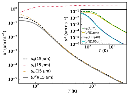
Figure 10: Estimates of the characteristic value of the drift velocity $u_{0}$ (dashed lines) as combination of the asymptotics trends given by $u^{H}$ (Eq. (118), dotted orange) and $u^{L}$ (Eq. (121), dotted red) for graphite samples having total length $l_{\rm TOT}=l_{L}+l_{R}=15\;\mu$m (main plot), 1 $\mu$m and 100 $\mu$m (inset). $\left<u^{x}\right>$ (solid lines) is the average value of the drift velocity computed from the numerical solution of the viscous heat equations in the region $l_{L}<x<(l_{L}+l_{R})$.

With these approximations, we can estimate the average value of the parabolic velocity profile, i.e. the characteristic value of the drift velocity at low temperatures $u_{L}$, as:

$$u_{L} =\left<u\right>=\frac{1}{w_{R}}\int_{0}^{w_{R}}u(y)dy=\frac{a\;w_{R}^{2}}{6}$$ (121)

where we used $w_{R}=6\;l$ and $l_{R}=8\;l$. We thus recover the expression for $u_{L}$ given in section VI in the main text. The average value of $u$ is interpolated in between the high and low temperature limit using Matthiessen’s rule, as: $u_{0}^{-1}=u_{H}^{-1}+u_{L}^{-1}$. The estimates of $u_{H}$, $u_{L}$ and $u_{0}$ for graphite are reported in Fig. 10. We also compare this rough estimate with the average value of ${u}^{x}(x,y)$ computed from the numerical solution of the viscous heat equations on the region $x>\frac{1}{5}l_{\rm TOT}$ of the geometry discussed in the main text and denoted denoted with $\left<u^{x}\right>$. Despite the qualitative arguments used to derive $u_{0}$, the estimate is able to capture qualitative trends and approximately reproduce average results from the numerical solution of the viscous heat equations.

Appendix I Hydrodynamic behavior in macroscopic diamond samples

In this section we show how extending the sizes in Fig. 5e up to 10 mm yields another peak for FDN for dimensions around 1 mm and temperatures around 50-60 K. This result has been confirmed by full solutions of the viscous heat equations similar to these reported in Fig. 5b. The increase of FDN at low temperature and large size reported in Fig. 11 is in qualitative agreement with the predictions for the second-sound window performed using the reduced isotropic crystal model or the Callaway model Khodusov and Naumovets (2012). However, in contrast with this work, Ref. Khodusov and Naumovets (2012) reports that an isotopic concentration much lower than the natural isotope abundance is necessary for the observation of second sound in diamond.

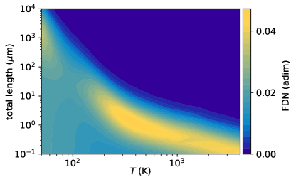
Figure 11: Hydrodynamic behavior in crystalline diamond at natural isotopic abundance: increasing the dimension of the diamond sample can yield an increase of the hydrodynamic effects at low temperatures.

The analysis here and in Fig. 5 are limited to a minimum reference temperature of $\bar{T}=50$ K because, for lower temperatures, anharmonicity becomes decreasingly smaller while size effects become increasingly larger, resulting in convergence issues for the numerical calculations (which would also require a refined, computationally-expensive, treatment of surface effects Cepellotti and Marzari (2017a)). Most importantly, the temperature/size range reported in Fig. 5 highlights the most accessible experimental conditions under which hydrodynamic behavior can appear in diamond, namely micrometer-sized diamond samples (thus much less expensive than millimeter-sized samples) and non-cryogenic temperatures.

Appendix J Computational details

First-principles calculations are performed with the Quantum ESPRESSO distribution Giannozzi et al. (2009, 2017). For all the materials analyzed, the LDA functional is used due to its capability to accurately describe the structural and vibrational Baroni et al. (2001) properties of graphite Fugallo et al. (2014), diamond Fugallo et al. (2013) and silicon Cepellotti and Marzari (2016), and its compatibility with the D3Q code Paulatto et al. (2013, 2015) for first-principles calculations of anharmonic (third-order) interatomic force constants. Details on the computation of the second- and third-order interatomic force constants are reported in Ref. Cepellotti and Marzari (2016) for silicon, in Ref. Fugallo et al. (2013) for diamond and in Ref. Fugallo et al. (2014) for graphite. The LBTE’s scattering matrix $\Omega_{\nu{\nu^{\prime}}}$ is computed as in Ref. Fugallo et al. (2013) and accounts for third-order anharmonicity Paulatto et al. (2013) and isotopic disorder Garg et al. (2011); Tamura (1983) at natural abundance. Thermal conductivity and viscosity calculations for silicon and diamond are performed using $27{\times}27{\times}27$ q-point grids and a Gaussian smearing of $2\;{\rm cm}^{-1}$ and $8\;{\rm cm}^{-1}$, respectively. Thermal conductivity and viscosity calculations for graphite are performed using a $49{\times}49{\times}3$ q-point grid and a Gaussian smearing of $8\;{\rm cm}^{-1}$. The use of an odd, Gamma-centered q-points mesh is crucial to correctly account for the parity symmetries of the scattering operator.

References

- Peierls (1929) R. Peierls, “Zur kinetischen theorie der wärmeleitung in kristallen,” Annalen der Physik 395, 1055–1101 (1929).
- Peierls (1955) R. E. Peierls, Quantum theory of solids (Oxford university press, 1955).
- Ziman (1960) J. M. Ziman, Electrons and phonons: the theory of transport phenomena in solids (Oxford university press, 1960).
- Mezhov-Deglin (1966) L. Mezhov-Deglin, “Measurement of the thermal conductivity of crystalline He4,” Soviet Phys. JETP 22 (1966).
- Ackerman et al. (1966) C. C. Ackerman, B. Bertman, H. A. Fairbank, and R. A. Guyer, “Second sound in solid helium,” Phys. Rev. Lett. 16, 789–791 (1966).
- Jackson et al. (1970) H. E. Jackson, C. T. Walker, and T. F. McNelly, “Second Sound in NaF,” Phys. Rev. Lett. 25, 26–28 (1970).
- Pohl and Irniger (1976) D. W. Pohl and V. Irniger, “Observation of Second Sound in NaF by Means of Light Scattering,” Phys. Rev. Lett. 36, 480–483 (1976).
- Narayanamurti and Dynes (1972) V. Narayanamurti and R. C. Dynes, “Observation of Second Sound in Bismuth,” Phys. Rev. Lett. 28, 1461–1465 (1972).
- Danil’Chenko et al. (1979) B. Danil’Chenko, V. Poroshin, and O. Sarbei, “An observation of second sound in sapphire,” JETP Lett 30 (1979).
- Hehlen et al. (1995) B. Hehlen, A.-L. Pérou, E. Courtens, and R. Vacher, “Observation of a Doublet in the Quasielastic Central Peak of Quantum-Paraelectric SrTi,” Phys. Rev. Lett. 75, 2416–2419 (1995).
- Koh and Cahill (2007) Y. K. Koh and D. G. Cahill, “Frequency dependence of the thermal conductivity of semiconductor alloys,” Phys. Rev. B 76, 075207 (2007).
- Bergamasco et al. (2018) L. Bergamasco, M. Alberghini, M. Fasano, A. Cardellini, E. Chiavazzo, and P. Asinari, “Mesoscopic moment equations for heat conduction: characteristic features and slow–fast mode decomposition,” Entropy 20, 126 (2018).
- Sussmann and Thellung (1963) J. A. Sussmann and A. Thellung, “Thermal Conductivity of Perfect Dielectric Crystals in the Absence of Umklapp Processes,” Proc. Phys. Soc. 81, 1122 (1963).
- Gurzhi (1964) R. Gurzhi, “Thermal conductivity of dielectrics and ferrodielectrics at low temperatures,” J. Exp. Theor. Phys. 46 (1964).
- Gurzhi (1968) R. N. Gurzhi, “Hydrodynamic effects in solids at low temperature,” Sov. Phys. Uspekhi 11, 255–270 (1968).
- Guyer and Krumhansl (1966a) R. A. Guyer and J. A. Krumhansl, “Solution of the linearized phonon boltzmann equation,” Phys. Rev. 148, 766–778 (1966a).
- Guyer and Krumhansl (1966b) R. A. Guyer and J. A. Krumhansl, “Thermal conductivity, second sound, and phonon hydrodynamic phenomena in nonmetallic crystals,” Phys. Rev. 148, 778–788 (1966b).
- Griffin (1965) A. Griffin, “On the detection of second sound in crystals by light scattering,” Phys. Lett. 17, 208–210 (1965).
- Enz (1968) C. P. Enz, “One-particle densities, thermal propagation, and second sound in dielectric crystals,” Ann. Phys. (N. Y.) 46, 114–173 (1968).
- Hardy (1970) R. J. Hardy, “Phonon boltzmann equation and second sound in solids,” Phys. Rev. B 2, 1193–1207 (1970).
- Hardy and Albers (1974) R. J. Hardy and D. L. Albers, “Hydrodynamic approximation to the phonon boltzmann equation,” Phys. Rev. B 10, 3546–3551 (1974).
- Omini and Sparavigna (1995) M. Omini and A. Sparavigna, “An iterative approach to the phonon Boltzmann equation in the theory of thermal conductivity,” Physica B: Condens. Matter 212, 101 – 112 (1995).
- Broido et al. (2007) D. A. Broido, M. Malorny, G. Birner, N. Mingo, and D. A. Stewart, “Intrinsic lattice thermal conductivity of semiconductors from first principles,” Appl. Phys. Lett. 91, 231922 (2007).
- Carrete et al. (2017) J. Carrete, B. Vermeersch, A. Katre, A. van Roekeghem, T. Wang, G. K. Madsen, and N. Mingo, “almaBTE : A solver of the space–time dependent Boltzmann transport equation for phonons in structured materials,” Comput. Phys. Commun. 220, 351 – 362 (2017).
- Fugallo et al. (2013) G. Fugallo, M. Lazzeri, L. Paulatto, and F. Mauri, “Ab initio variational approach for evaluating lattice thermal conductivity,” Phys. Rev. B 88, 045430 (2013).
- Chaput (2013) L. Chaput, “Direct Solution to the Linearized Phonon Boltzmann Equation,” Phys. Rev. Lett. 110, 265506 (2013).
- Cepellotti and Marzari (2016) A. Cepellotti and N. Marzari, “Thermal Transport in Crystals as a Kinetic Theory of Relaxons,” Phys. Rev. X 6, 041013 (2016).
- Esfarjani et al. (2011) K. Esfarjani, G. Chen, and H. T. Stokes, “Heat transport in silicon from first-principles calculations,” Phys. Rev. B 84, 085204 (2011).
- Luckyanova et al. (2012) M. N. Luckyanova, J. Garg, K. Esfarjani, A. Jandl, M. T. Bulsara, A. J. Schmidt, A. J. Minnich, S. Chen, M. S. Dresselhaus, Z. Ren, E. A. Fitzgerald, and G. Chen, “Coherent phonon heat conduction in superlattices,” Science 338, 936–939 (2012).
- Cahill et al. (2014) D. G. Cahill, P. V. Braun, G. Chen, D. R. Clarke, S. Fan, K. E. Goodson, P. Keblinski, W. P. King, G. D. Mahan, A. Majumdar, H. J. Maris, S. R. Phillpot, E. Pop, and L. Shi, “Nanoscale thermal transport. ii. 2003–2012,” Appl. Phys. Rev. 1, 011305 (2014).
- Cepellotti et al. (2015) A. Cepellotti, G. Fugallo, L. Paulatto, M. Lazzeri, F. Mauri, and N. Marzari, “Phonon hydrodynamics in two-dimensional materials,” Nat. Commun. 6, 6400 (2015).
- Paulatto et al. (2013) L. Paulatto, F. Mauri, and M. Lazzeri, “Anharmonic properties from a generalized third-order ab initio approach: Theory and applications to graphite and graphene,” Phys. Rev. B 87, 214303 (2013).
- Paulatto et al. (2015) L. Paulatto, I. Errea, M. Calandra, and F. Mauri, “First-principles calculations of phonon frequencies, lifetimes, and spectral functions from weak to strong anharmonicity: The example of palladium hydrides,” Phys. Rev. B 91, 054304 (2015).
- Lindsay (2016) L. Lindsay, “First Principles Peierls-Boltzmann Phonon Thermal Transport: A Topical Review,” Nanosc. Microsc. Therm. 20, 67–84 (2016).
- Cepellotti and Marzari (2017a) A. Cepellotti and N. Marzari, “Boltzmann Transport in Nanostructures as a Friction Effect,” Nano Lett. (2017a).
- Omini and Sparavigna (1996) M. Omini and A. Sparavigna, “Beyond the isotropic-model approximation in the theory of thermal conductivity,” Phys. Rev. B 53, 9064–9073 (1996).
- McGaughey et al. (2019) A. J. McGaughey, A. Jain, H.-Y. Kim, and B. Fu, “Phonon properties and thermal conductivity from first principles, lattice dynamics, and the boltzmann transport equation,” J. Appl. Phys. 125, 011101 (2019).
- Simoncelli, M. and Marzari, N. and Mauri, F. (2019) Simoncelli, M. and Marzari, N. and Mauri, F., “Unified theory of thermal transport in crystals and glasses,” Nat. Phys. 15, 809–813 (2019).
- Lee et al. (2015) S. Lee, D. Broido, K. Esfarjani, and G. Chen, “Hydrodynamic phonon transport in suspended graphene,” Nat. Commun. 6, 6290 (2015).
- Cepellotti and Marzari (2017b) A. Cepellotti and N. Marzari, “Transport waves as crystal excitations,” Phys. Rev. Materials 1, 045406 (2017b).
- Lee and Lindsay (2017) S. Lee and L. Lindsay, “Hydrodynamic phonon drift and second sound in a (20,20) single-wall carbon nanotube,” Phys. Rev. B 95 (2017).
- Ding et al. (2018) Z. Ding, J. Zhou, B. Song, V. Chiloyan, M. Li, T.-H. Liu, and G. Chen, “Phonon Hydrodynamic Heat Conduction and Knudsen Minimum in Graphite,” Nano Lett. 18, 638–649 (2018).
- Huberman et al. (2019) S. Huberman, R. A. Duncan, K. Chen, B. Song, V. Chiloyan, Z. Ding, A. A. Maznev, G. Chen, and K. A. Nelson, “Observation of second sound in graphite at temperatures above 100 k,” Science 364, 375–379 (2019).
- Martelli et al. (2018) V. Martelli, J. L. Jiménez, M. Continentino, E. Baggio-Saitovitch, and K. Behnia, “Thermal Transport and Phonon Hydrodynamics in Strontium Titanate,” Phys. Rev. Lett. 120 (2018).
- Khodusov and Naumovets (2012) V. Khodusov and A. Naumovets, “Second sound waves in diamond,” Diam. Relat. Mater. 21, 92 – 98 (2012).
- Machida et al. (2018) Y. Machida, A. Subedi, K. Akiba, A. Miyake, M. Tokunaga, Y. Akahama, K. Izawa, and K. Behnia, “Observation of Poiseuille flow of phonons in black phosphorus,” Sci. Adv. 4 (2018).
- Hua and Minnich (2014) C. Hua and A. J. Minnich, “Analytical Green’s function of the multidimensional frequency-dependent phonon Boltzmann equation,” Phys. Rev. B 90, 214306 (2014).
- Vermeersch et al. (2015) B. Vermeersch, J. Carrete, N. Mingo, and A. Shakouri, “Superdiffusive heat conduction in semiconductor alloys. I. Theoretical foundations,” Phys. Rev. B 91, 085202 (2015).
- Maznev et al. (2011) A. A. Maznev, J. A. Johnson, and K. A. Nelson, “Onset of nondiffusive phonon transport in transient thermal grating decay,” Phys. Rev. B 84, 195206 (2011).
- Yang and Dames (2015) F. Yang and C. Dames, “Heating-frequency-dependent thermal conductivity: An analytical solution from diffusive to ballistic regime and its relevance to phonon scattering measurements,” Phys. Rev. B 91, 165311 (2015).
- Péraud and Hadjiconstantinou (2016) J.-P. M. Péraud and N. G. Hadjiconstantinou, “Extending the range of validity of Fourier’s law into the kinetic transport regime via asymptotic solution of the phonon Boltzmann transport equation,” Phys. Rev. B 93, 045424 (2016).
- Chen (2001) G. Chen, “Ballistic-diffusive heat-conduction equations,” Phys. Rev. Lett. 86, 2297–2300 (2001).
- Anderson and Tamma (2006) C. V. D. R. Anderson and K. K. Tamma, “Novel Heat Conduction Model for Bridging Different Space and Time Scales,” Phys. Rev. Lett. 96, 184301 (2006).
- Ordonez-Miranda et al. (2011) J. Ordonez-Miranda, R. Yang, and J. Alvarado-Gil, “A constitutive equation for nano-to-macro-scale heat conduction based on the boltzmann transport equation,” J. Appl. Phys. 109, 084319 (2011).
- Ramu and Ma (2014) A. T. Ramu and Y. Ma, “An enhanced fourier law derivable from the boltzmann transport equation and a sample application in determining the mean-free path of nondiffusive phonon modes,” J. Appl. Phys. 116, 093501 (2014).
- Hua et al. (2019) C. Hua, L. Lindsay, X. Chen, and A. Minnich, “Experimental demonstration of a generalized Fourier’s Law for non-diffusive thermal transport,” arXiv preprint arXiv:1902.10020 (2019).
- Cao and Guo (2007) B.-Y. Cao and Z.-Y. Guo, “Equation of motion of a phonon gas and non-Fourier heat conduction,” J. Appl. Phys. 102, 053503 (2007).
- Alvarez et al. (2009) F. Alvarez, D. Jou, and A. Sellitto, “Phonon hydrodynamics and phonon-boundary scattering in nanosystems,” J. Appl. Phys. 105, 014317 (2009).
- Guo and Wang (2015) Y. Guo and M. Wang, “Phonon hydrodynamics and its applications in nanoscale heat transport,” Phys. Rep. 595, 1–44 (2015).
- Guo and Wang (2018) Y. Guo and M. Wang, “Phonon hydrodynamics for nanoscale heat transport at ordinary temperatures,” Phys. Rev. B 97, 035421 (2018).
- Ziabari et al. (2018) A. Ziabari, P. Torres, B. Vermeersch, Y. Xuan, X. Cartoixà, A. Torelló, J.-H. Bahk, Y. R. Koh, M. Parsa, P. D. Ye, F. X. Alvarez, and A. Shakouri, “Full-field thermal imaging of quasiballistic crosstalk reduction in nanoscale devices,” Nat. Commun. 9 (2018).
- Torres et al. (2018) P. Torres, A. Ziabari, A. Torelló, J. Bafaluy, J. Camacho, X. Cartoixà, A. Shakouri, and F. X. Alvarez, “Emergence of hydrodynamic heat transport in semiconductors at the nanoscale,” Phys. Rev. Materials 2, 076001 (2018).
- Li and Lee (2018) X. Li and S. Lee, “Role of hydrodynamic viscosity on phonon transport in suspended graphene,” Phys. Rev. B 97, 094309 (2018).
- Note (1) i.e. the unit cell volume times the number of unit cells that constitute the crystal . is also the number of wavevectors used to sample the Brillouin zone.
- Klemens and Simon (1951) P. G. Klemens and F. E. Simon, “The thermal conductivity of dielectric solids at low temperatures (theoretical),” Proc. Royal Soc. Lond. Series A. 208, 108–133 (1951).
- Rice (1967) M. J. Rice, “Theory of viscosity in nearly ferromagnetic fermi liquids,” Phys. Rev. 162, 189–191 (1967).
- Allen and Perebeinos (2018) P. B. Allen and V. Perebeinos, “Temperature in a Peierls-Boltzmann treatment of nonlocal phonon heat transport,” Phys. Rev. B 98, 085427 (2018).
- Note (2) This follows from the property .
- Fugallo et al. (2014) G. Fugallo, A. Cepellotti, L. Paulatto, M. Lazzeri, N. Marzari, and F. Mauri, “Thermal Conductivity of Graphene and Graphite: Collective Excitations and Mean Free Paths,” Nano Lett. 14, 6109–6114 (2014).
- Gandolfi et al. (2019) M. Gandolfi, G. Benetti, C. Glorieux, C. Giannetti, and F. Banfi, “Accessing temperature waves: A dispersion relation perspective,” Int. J. Heat Mass Transf. 143, 118553 (2019).
- Torres et al. (2017) P. Torres, A. Torelló, J. Bafaluy, J. Camacho, X. Cartoixà, and F. X. Alvarez, “First principles kinetic-collective thermal conductivity of semiconductors,” Phys. Rev. B 95, 165407 (2017).
- Heron et al. (2009) J. Heron, T. Fournier, N. Mingo, and O. Bourgeois, “Mesoscopic size effects on the thermal conductance of silicon nanowire,” Nano Lett. 9, 1861–1865 (2009).
- Siemens et al. (2010) M. E. Siemens, Q. Li, R. Yang, K. A. Nelson, E. H. Anderson, M. M. Murnane, and H. C. Kapteyn, “Quasi-ballistic thermal transport from nanoscale interfaces observed using ultrafast coherent soft x-ray beams,” Nat. Mater. 9, 26 (2010).
- Johnson et al. (2013) J. A. Johnson, A. A. Maznev, J. Cuffe, J. K. Eliason, A. J. Minnich, T. Kehoe, C. M. S. Torres, G. Chen, and K. A. Nelson, “Direct measurement of room-temperature nondiffusive thermal transport over micron distances in a silicon membrane,” Phys. Rev. Lett. 110, 025901 (2013).
- Regner et al. (2013) K. T. Regner, D. P. Sellan, Z. Su, C. H. Amon, A. J. McGaughey, and J. A. Malen, “Broadband phonon mean free path contributions to thermal conductivity measured using frequency domain thermoreflectance,” Nat. Commun. 4, 1640 (2013).
- Wilson and Cahill (2014) R. B. Wilson and D. G. Cahill, “Anisotropic failure of Fourier theory in time-domain thermoreflectance experiments,” Nat. Commun. 5, 5075 (2014).
- Péraud and Hadjiconstantinou (2011) J.-P. M. Péraud and N. G. Hadjiconstantinou, “Efficient simulation of multidimensional phonon transport using energy-based variance-reduced Monte Carlo formulations,” Phys. Rev. B 84, 205331 (2011).
- Sun and Allen (2010) T. Sun and P. B. Allen, “Lattice thermal conductivity: Computations and theory of the high-temperature breakdown of the phonon-gas model,” Phys. Rev. B 82, 224305 (2010).
- Berman (1992) R. Berman, “Thermal conductivity of isotopically enriched diamonds,” Phys. Rev. B 45, 5726–5728 (1992).
- Onn et al. (1992) D. G. Onn, A. Witek, Y. Z. Qiu, T. R. Anthony, and W. F. Banholzer, “Some aspects of the thermal conductivity of isotopically enriched diamond single crystals,” Phys. Rev. Lett. 68, 2806–2809 (1992).
- Olson et al. (1993) J. R. Olson, R. O. Pohl, J. W. Vandersande, A. Zoltan, T. R. Anthony, and W. F. Banholzer, “Thermal conductivity of diamond between 170 and 1200 K and the isotope effect,” Phys. Rev. B 47, 14850–14856 (1993).
- Wei et al. (1993) L. Wei, P. K. Kuo, R. L. Thomas, T. R. Anthony, and W. F. Banholzer, “Thermal conductivity of isotopically modified single crystal diamond,” Phys. Rev. Lett. 70, 3764–3767 (1993).
- Ward et al. (2009) A. Ward, D. A. Broido, D. A. Stewart, and G. Deinzer, “Ab initio theory of the lattice thermal conductivity in diamond,” Phys. Rev. B 80, 125203 (2009).
- Broido et al. (2012) D. A. Broido, L. Lindsay, and A. Ward, “Thermal conductivity of diamond under extreme pressure: A first-principles study,” Phys. Rev. B 86, 115203 (2012).
- Inyushkin et al. (2018) A. V. Inyushkin, A. N. Taldenkov, J. W. Ager III, E. E. Haller, H. Riemann, N. V. Abrosimov, H.-J. Pohl, and P. Becker, “Ultrahigh thermal conductivity of isotopically enriched silicon,” J. Appl. Phys. 123, 095112 (2018).
- Lifshitz and Pitaevskii (1981) E. M. Lifshitz and L. P. Pitaevskii, Physical Kinetics. Course of theoretical physics. Vol. 10 (Pergamon Press, Oxford, 1981).
- Bonini et al. (2012) N. Bonini, J. Garg, and N. Marzari, “Acoustic phonon lifetimes and thermal transport in free-standing and strained graphene,” Nano letters 12, 2673–2678 (2012).
- Mariani and von Oppen (2008) E. Mariani and F. von Oppen, “Flexural Phonons in Free-Standing Graphene,” Phys. Rev. Lett. 100, 076801 (2008).
- Ong and Pop (2011) Z.-Y. Ong and E. Pop, “Effect of substrate modes on thermal transport in supported graphene,” Phys. Rev. B 84, 075471 (2011).
- Weinbub and Ferry (2018) J. Weinbub and D. K. Ferry, “Recent advances in Wigner function approaches,” Appl. Phys. Rev. 5, 041104 (2018).
- Logan (2014) J. D. Logan, Applied partial differential equations (Springer, 2014).
- Kwok (1967) P. C. Kwok, “Dispersion and damping of second sound in non-isotropic solids,” Physics Physique Fizika 3, 221 (1967).
- Ackerman and Guyer (1968) C. Ackerman and R. Guyer, “Temperature pulses in dielectric solids,” Ann. Phys. (N. Y.) 50, 128–185 (1968).
- Maris (1981a) H. J. Maris, “Second sound and heat flow in anisotropic solids,” Phys. Rev. B 24, 1205–1208 (1981a).
- Chester (1963) M. Chester, “Second sound in solids,” Phys. Rev. 131, 2013–2015 (1963).
- Cattaneo (1948) C. Cattaneo, “Sulla conduzione del calore,” Atti Sem. Mat. Fis. Univ. Modena 3, 83–101 (1948).
- Joseph and Preziosi (1989) D. D. Joseph and L. Preziosi, “Heat waves,” Rev. Mod. Phys. 61, 41–73 (1989).
- Tzou (1995) D. Y. Tzou, “The generalized lagging response in small-scale and high-rate heating,” Int. J. Heat Mass Transf. 38, 3231–3240 (1995).
- Allen (2013) P. B. Allen, “Improved Callaway model for lattice thermal conductivity,” Phys. Rev. B 88, 144302 (2013).
- Lepri et al. (2003) S. Lepri, R. Livi, and A. Politi, “Thermal conduction in classical low-dimensional lattices,” Phys. Rep. 377, 1–80 (2003).
- Inc. (2016) W. R. Inc., “Mathematica, Version 11.3,” (2016), champaign, IL, 2018.
- Maris (1981b) H. J. Maris, “Second sound and heat flow in anisotropic solids,” Phys. Rev. B 24, 1205–1208 (1981b).
- Simons (1983) S. Simons, “The relation between the heat current and the phonon drift velocity,” Am. J. Phys. 51, 457–458 (1983).
- Schelling et al. (2002) P. K. Schelling, S. R. Phillpot, and P. Keblinski, “Comparison of atomic-level simulation methods for computing thermal conductivity,” Phys. Rev. B 65, 144306 (2002).
- Zhang et al. (2017) Y.-Y. Zhang, Q.-X. Pei, H.-Y. Liu, and N. Wei, “Thermal conductivity of a h-BCN monolayer,” Phys. Chem. Chem. Phys. 19, 27326–27331 (2017).
- Khadem and Wemhoff (2013) M. H. Khadem and A. P. Wemhoff, “Comparison of Green–Kubo and NEMD heat flux formulations for thermal conductivity prediction using the Tersoff potential,” Comput. Mater. Sci. 69, 428–434 (2013).
- Puligheddu et al. (2017) M. Puligheddu, F. Gygi, and G. Galli, “First-principles simulations of heat transport,” Phys. Rev. Materials 1, 060802 (2017).
- Iubini et al. (2018) S. Iubini, P. Di Cintio, S. Lepri, R. Livi, and L. Casetti, “Heat transport in oscillator chains with long-range interactions coupled to thermal reservoirs,” Phys. Rev. E 97, 032102 (2018).
- He et al. (2012) Y. He, I. Savić, D. Donadio, and G. Galli, “Lattice thermal conductivity of semiconducting bulk materials: atomistic simulations,” Phys. Chem. Chem. Phys. 14, 16209–16222 (2012).
- Zhou et al. (2009) X. W. Zhou, S. Aubry, R. E. Jones, A. Greenstein, and P. K. Schelling, “Towards more accurate molecular dynamics calculation of thermal conductivity: Case study of gan bulk crystals,” Phys. Rev. B 79, 115201 (2009).
- Fan et al. (2017) Z. Fan, L. F. C. Pereira, P. Hirvonen, M. M. Ervasti, K. R. Elder, D. Donadio, T. Ala-Nissila, and A. Harju, “Thermal conductivity decomposition in two-dimensional materials: Application to graphene,” Phys. Rev. B 95, 144309 (2017).
- Allen (2018) P. B. Allen, “Analysis of nonlocal phonon thermal conductivity simulations showing the ballistic to diffusive crossover,” Phys. Rev. B 97, 134307 (2018).
- Li et al. (2019) Z. Li, S. Xiong, C. Sievers, Y. Hu, Z. Fan, N. Wei, H. Bao, S. Chen, D. Donadio, and T. Ala-Nissila, “Influence of Boundaries and Thermostatting on Nonequilibrium Molecular Dynamics Simulations of Heat Conduction in Solids,” arXiv preprint arXiv:1905.11024 (2019).
- Li et al. (2014) W. Li, J. Carrete, N. A. Katcho, and N. Mingo, “ShengBTE: A solver of the Boltzmann transport equation for phonons,” Comput. Phys. Commun. 185, 1747 – 1758 (2014).
- Buckingham (1914) E. Buckingham, “On physically similar systems; illustrations of the use of dimensional equations,” Phys. Rev. 4, 345–376 (1914).
- White (2003) F. M. White, “Fluid mechanics. 5th edition,” Boston: McGraw-Hill Book Company (2003).
- Maassen and Lundstrom (2015) J. Maassen and M. Lundstrom, “Steady-state heat transport: Ballistic-to-diffusive with Fourier’s law,” J. Appl. Phys. 117, 035104 (2015).
- Terraneo et al. (2002) M. Terraneo, M. Peyrard, and G. Casati, “Controlling the energy flow in nonlinear lattices: A model for a thermal rectifier,” Phys. Rev. Lett. 88, 094302 (2002).
- Li et al. (2004) B. Li, L. Wang, and G. Casati, “Thermal diode: Rectification of heat flux,” Phys. Rev. Lett. 93, 184301 (2004).
- Chang et al. (2006) C. W. Chang, D. Okawa, A. Majumdar, and A. Zettl, “Solid-state thermal rectifier,” Science 314, 1121–1124 (2006).
- Hu et al. (2009) J. Hu, X. Ruan, and Y. P. Chen, “Thermal conductivity and thermal rectification in graphene nanoribbons: a molecular dynamics study,” Nano Lett. 9, 2730–2735 (2009).
- Wang et al. (2014) Y. Wang, A. Vallabhaneni, J. Hu, B. Qiu, Y. P. Chen, and X. Ruan, “Phonon lateral confinement enables thermal rectification in asymmetric single-material nanostructures,” Nano Lett. 14, 592–596 (2014).
- Anufriev and Nomura (2015) R. Anufriev and M. Nomura, “Thermal conductance boost in phononic crystal nanostructures,” Phys. Rev. B 91, 245417 (2015).
- Volz et al. (2016) S. Volz, J. Ordonez-Miranda, A. Shchepetov, M. Prunnila, J. Ahopelto, T. Pezeril, G. Vaudel, V. Gusev, P. Ruello, E. M. Weig, M. Schubert, M. Hettich, M. Grossman, T. Dekorsy, F. Alzina, B. Graczykowski, E. Chavez-Angel, J. Sebastian Reparaz, M. R. Wagner, C. M. Sotomayor-Torres, S. Xiong, S. Neogi, and D. Donadio, “Nanophononics: state of the art and perspectives,” The European Physical Journal B 89, 15 (2016).
- Wang et al. (2017) H. Wang, S. Hu, K. Takahashi, X. Zhang, H. Takamatsu, and J. Chen, “Experimental study of thermal rectification in suspended monolayer graphene,” Nat. Commun. 8, 15843 (2017).
- Liu et al. (2017) Y. Liu, Y. Xu, S.-C. Zhang, and W. Duan, “Model for topological phononics and phonon diode,” Phys. Rev. B 96, 064106 (2017).
- Chen et al. (2018) S. Chen, D. Donadio, G. Benenti, and G. Casati, “Efficient thermal diode with ballistic spacer,” Phys. Rev. E 97, 030101 (2018).
- Felix and Pereira (2018) I. M. Felix and L. F. C. Pereira, “Thermal conductivity of graphene-hbn superlattice ribbons,” Sci. Rep. 8, 2737 (2018).
- Sood et al. (2018) A. Sood, F. Xiong, S. Chen, H. Wang, D. Selli, J. Zhang, C. J. McClellan, J. Sun, D. Donadio, Y. Cui, et al., “An electrochemical thermal transistor,” Nat. Commun. 9, 4510 (2018).
- De Luca et al. (2019) M. De Luca, C. Fasolato, M. A. Verheijen, Y. Ren, M. Y. Swinkels, S. Koelling, E. P. Bakkers, R. Rurali, X. Cartoixa, and I. Zardo, “Phonon engineering in twinning superlattice nanowires,” Nano Lett. (2019).
- Levitov and Falkovich (2016) L. Levitov and G. Falkovich, “Electron viscosity, current vortices and negative nonlocal resistance in graphene,” Nat. Phys. 12, 672 (2016).
- Bandurin et al. (2016) D. A. Bandurin, I. Torre, R. K. Kumar, M. Ben Shalom, A. Tomadin, A. Principi, G. H. Auton, E. Khestanova, K. S. Novoselov, I. V. Grigorieva, L. A. Ponomarenko, A. K. Geim, and M. Polini, “Negative local resistance caused by viscous electron backflow in graphene,” Science 351, 1055–1058 (2016).
- Moll et al. (2016) P. J. Moll, P. Kushwaha, N. Nandi, B. Schmidt, and A. P. Mackenzie, “Evidence for hydrodynamic electron flow in PdCoO2,” Science 351, 1061–1064 (2016).
- Scaffidi et al. (2017) T. Scaffidi, N. Nandi, B. Schmidt, A. P. Mackenzie, and J. E. Moore, “Hydrodynamic electron flow and hall viscosity,” Phys. Rev. Lett. 118, 226601 (2017).
- Spohn (2006) H. Spohn, “The phonon Boltzmann equation, properties and link to weakly anharmonic lattice dynamics,” J. Stat. Phys. 124, 1041–1104 (2006).
- Hardy (1963) R. J. Hardy, “Energy-flux operator for a lattice,” Phys. Rev. 132, 168–177 (1963).
- Hardy (1965) R. J. Hardy, “Lowest-order contribution to the lattice thermal conductivity,” J. Math. Phys. 6, 1749–1761 (1965).
- Giannozzi et al. (2009) P. Giannozzi, S. Baroni, N. Bonini, M. Calandra, R. Car, C. Cavazzoni, D. Ceresoli, G. L. Chiarotti, M. Cococcioni, I. Dabo, A. D. Corso, S. de Gironcoli, S. Fabris, G. Fratesi, R. Gebauer, U. Gerstmann, C. Gougoussis, A. Kokalj, M. Lazzeri, L. Martin-Samos, N. Marzari, F. Mauri, R. Mazzarello, S. Paolini, A. Pasquarello, L. Paulatto, C. Sbraccia, S. Scandolo, G. Sclauzero, A. P. Seitsonen, A. Smogunov, P. Umari, and R. M. Wentzcovitch, “QUANTUM ESPRESSO: a modular and open-source software project for quantum simulations of materials,” J. Phys. Condens. Matter 21, 395502 (2009).
- Giannozzi et al. (2017) P. Giannozzi, O. Andreussi, T. Brumme, O. Bunau, M. B. Nardelli, M. Calandra, R. Car, C. Cavazzoni, D. Ceresoli, M. Cococcioni, N. Colonna, I. Carnimeo, A. D. Corso, S. de Gironcoli, P. Delugas, R. A. D. Jr, A. Ferretti, A. Floris, G. Fratesi, G. Fugallo, R. Gebauer, U. Gerstmann, F. Giustino, T. Gorni, J. Jia, M. Kawamura, H.-Y. Ko, A. Kokalj, E. Küçükbenli, M. Lazzeri, M. Marsili, N. Marzari, F. Mauri, N. L. Nguyen, H.-V. Nguyen, A. O. de-la Roza, L. Paulatto, S. Poncé, D. Rocca, R. Sabatini, B. Santra, M. Schlipf, A. P. Seitsonen, A. Smogunov, I. Timrov, T. Thonhauser, P. Umari, N. Vast, X. Wu, and S. Baroni, “Advanced capabilities for materials modelling with Quantum ESPRESSO,” J. Phys. Condens. Matter 29, 465901 (2017).
- Baroni et al. (2001) S. Baroni, S. de Gironcoli, A. Dal Corso, and P. Giannozzi, “Phonons and related crystal properties from density-functional perturbation theory,” Rev. Mod. Phys. 73, 515–562 (2001).
- Garg et al. (2011) J. Garg, N. Bonini, B. Kozinsky, and N. Marzari, “Role of Disorder and Anharmonicity in the Thermal Conductivity of Silicon-Germanium Alloys: A First-Principles Study,” Phys. Rev. Lett. 106, 045901 (2011).
- Tamura (1983) S.-i. Tamura, “Isotope scattering of dispersive phonons in Ge,” Phys. Rev. B 27, 858–866 (1983).