Localisation and transport in bidimensional random models with separable Hamiltonians

Abstract

We consider two bidimensional random models characterised by the following features: a) their Hamiltonians are separable in polar coordinates and b) the random part of the potential depends either on the angular coordinate or on the radial one, but not on both. The disorder correspondingly localises the angular or the radial part of the eigenfunctions. We analyse the analogies and the differences which exist between the selected 2D models and their 1D counterparts. We show how the analogies allow one to use correlated disorder to design a localisation length with pre-defined energy dependence and to produce directional localisation of the wavefunctions in models with angular disorder. We also discuss the importance of finite-size and resonance effects in shaping the eigenfunctions of the model with angular disorder; for the model with disorder associated to the radial variable we show under what conditions the localisation length coincides with the expression valid in the 1D case.

1 Introduction

In the sixty years elapsed since the publication of the pioneering Anderson paper [1], the phenomenon of Anderson localisation has been intensively studied (see, e.g., [2, 3, 4, 5] and references therein). Although the theory was initially conceived within the field of condensed-matter physics, the realisation that destructive interference is the mechanism underlying the Anderson localisation of electronic states has led to the application of the Anderson theory to a large number of fields, including mesoscopic physics [6], propagation of electromagnetic and acoustic waves [7, 8, 9, 10, 11], experiments with cold atoms [12, 13, 14, 15, 16, 17, 18, 19, 20, 21]. Even light localisation was considered [22, 23, 24], although it should be noted that localisation of electromagnetic waves in three dimensions was recently questioned [25] and that experimental reports of light localisation in three dimensions seem to be based on incorrect interpretations of the data [26].

In the theoretical study of Anderson localisation, a special role has been played by one-dimensional (1D) models, which are more amenable to analytical treatment than their 2D and 3D counterparts. The practical applicability of 1D models, however, is often reduced because many results which can be proved for this class of systems are not valid in higher dimensions. It has long been known, for instance, that in 1D models any amount of uncorrelated disorder leads to the localisation of all electronic states [27] so that, contrary to what happens in three dimensions, no metal-insulator transition can occur in 1D models. The situation is more complex in the case of correlated disorder: in fact, specific long-range correlations of the disorder can produce an effective metal-insulator transition even in 1D models [28]. The peculiar features of 1D systems imply that a direct study of 2D and 3D models cannot be avoided in order to reach a full understanding of Anderson localisation.

Few analytical results have been obtained for 2D and 3D models. A crucial tool for the understanding of these models is represented by the single-parameter scaling (SPS) theory, which was introduced in [29, 30] and still provides an essential framework for the study of Anderson localisation. The SPS theory predicts that, for uncorrelated disorder, all states are localised in 1D and 2D models, whereas a metal-insulator transition occurs in 3D systems. Two is the lower critical dimension and, for the standard Anderson model without spin-dependent terms, the scaling hypothesis leads to the conclusion that all states are localised, although their localisation length may be exponentially large for weak disorder [31]. This is the generally accepted view, although there has always been a certain amount of controversy concerning the possibility of a metallic phase in 2D models even in the absence of a magnetic field (see [32] and references therein).

Immediately after the publication of the original SPS paper [29], diagrammatic techniques were used to show that in 2D models the conductivity depends logarithmically on the frequency in the low-frequency regime [33]. In the early ’80s the scaling hypothesis was corroborated by numerical results obtained by MacKinnon and Kramer [34]. At the same time, numerical studies of 2D models were also carried out in order to confirm the predictions of the SPS theory [35]. In the ’90s Schreiber and coworkers used numerical techniques to perform comprehensive studies of the 2D Anderson model with diagonal and off-diagonal disorder [36, 37, 38]. They analysed the properties of the eigenstates and the density of states using an approach based on the transfer matrix method. Transfer matrix methods were also used in more recent numerical studies of the localisation length in 2D models with diagonal and off-diagonal disorder [39]. More recently, the use of a generalised form of the DPMK equation [40, 41] was proposed to study 2D models [42].

The works on 2D models mentioned so far did not consider disorder with spatial correlations. This subject received attention in a series of papers [43, 44, 45, 46] focused on models with disorder having a power-law spectral density $S(k)\sim 1/k^{\alpha}$. For strongly correlated disorder, these studies generally show that extended states and ballistic diffusion processes emerge. In the field of cold atoms, the use of correlated disorder to produce spectral shaping of the localisation length in 2D and 3D experiments was considered in [47, 48]. More recently, the effects of short-range correlations were considered for a Bose gas confined on a 2D square lattice [49]. Using a 2D generalisation of the dual dimer random model, the authors showed that short-range correlations of the disorder can enhance quantum coherence in a weakly interacting many-body system.

In this paper we focus our interest on two bidimensional models. To avoid the rather intractable problems which present themselves whenever one tries to obtain analytical results for 2D systems, we considered models with two specific features: a) we selected models with separable Hamiltonians in polar coordinates and b) we picked potentials with a random part depending either on the angle or the radial variable, but not on both coordinates at the same time, thus keeping the separability. This choice allowed us to reduce the study of 2D models to the analysis of associated 1D systems and thus obtain a deeper understanding of the effects of disorder.

In particular we found that, when the random potential depends on the angle variable, it is the angular part of the wavefunctions which is localised; conversely, when disorder varies with the radial variable, it is the radial part of the wavefunction which suffers localisation. Although this might seem as a foregone conclusion, we would like to stress that the reduction of 2D models to systems of lower dimensionality is far from trivial. In fact, we found that the study of models with angular disorder requires a careful analysis of finite-size effects, which cannot be avoided since the angle variable has a necessarily finite domain; we also discovered that resonances can play an important role in 2D Kronig-Penney models with angular disorder. The analysis of models with radial disorder, on the other hand, revealed that 2D models with a central random potential can be effectively reduced to their 1D homologues only if the potential does not decrease too quickly away from the force centre.

Throughout the paper, we considered the case of correlated disorder. For the model with disorder associated to the angular variable, we found that correlated disorder can be extremely useful to enhance localisation and compensate for the fact that the geometry of the problem sets limits on the strength of structural disorder. This is also an issue for experimental realisations which always involve finite-size systems. In the case of disorder depending on the radial coordinate, we found that spatial correlations can be used to modulate the transmission properties of the model within the allowed energy bands.

We think that the theoretical understanding of the relevant features of the studied models has a twofold importance: it sheds some light on the difficult problem of localisation in 2D systems and makes possible to design actual devices which can be used to filter and focus waves as desired.

The paper is organised as follows. We introduce the separable models discussed in this work in Sec. 2. We devote Sec. 3 to the discussion of a 2D model with a random potential that depends only on the angle variable. We show how a disorder of this kind produces localisation of the angular part of the wavefunction and we analyse in detail the effects due to the finite size and geometrical constraints of the model. Correlated disorder is applied to enhance the localisation in angular direction. We show that all radial bands localise in the same direction (see figure 13); this feature suggests that such models might be used to implement directional transport. In Sec. 4 we shift our attention to a model with a central random potential. In this case it is the radial component of the eigenstates which is localised. We show how one can use spatial correlations of the disorder to allow transmission in predefined energy windows. We present our conclusions in Sec. 5.

2 Separable models in two dimensions

We consider a quantum particle in a two-dimensional plane. The particle wavefunction obeys the Schrödinger equation

$$\left[-\nabla^{2}+U(r,\theta)\right]\psi(r,\theta)=E\psi(r,\theta)$$ (1)

where the symbol $\nabla^{2}$ represents the 2D Laplacian which, in polar coordinates, can be written as

$$\nabla^{2}=\frac{1}{r}\frac{\partial}{\partial r}\left(r\frac{\partial}{\partial r}\right)+\frac{1}{r^{2}}\frac{\partial^{2}}{\partial\theta^{2}}.$$ (2)

In Eq. (1) we used energy units such that $\hbar^{2}/2m=1$; we shall follow this convention throughout the rest of the paper.

As a full analytical treatment of arbitrary random potentials with spatial correlations is out of reach, we focused our attention on systems which are separable in $r$ and $\theta$. This choice simplifies the mathematical problem, because in this case the wave function can be expressed in the factorised form

$$\psi(r,\theta)=R(r)\Theta(\theta)$$ (3)

and the Schrödinger equation (1) splits in a pair of 1D differential equations.

From a physical point of view, we study two separable models in which randomness is introduced either via the angular variable $\theta$ or through the radial variable $r$. Thus we assume the random potential in Eq. 1 to have the form:

$$U(r,\theta)=\left\{\begin{array}[]{cl}\displaystyle\frac{1}{r^{2}}V_{1}(\theta)&\mbox{ for angular randomness,}\\ V_{2}(r)&\mbox{ for radial randomness.}\\ \end{array}\right.$$ (4)

We consider functions $V_{1}(\theta)$ and $V_{2}(r)$ constituted by sums of random $\delta$-barriers, so that in both cases our analysis will involve the study of variants of the aperiodic Kronig-Penney model. We specify the exact form of the potential (4) in Sec. 3.1 for the case of angular disorder and in Sec. 4.1 for the case of radial disorder.

3 Angle-dependent disorder

3.1 Model with angle-dependent disorder

We consider a quantum particle confined in an annulus on a two-dimensional plane. We use the symbols $r_{1}$ and $r_{2}$ to denote the inner and outer radii of the annulus, where $r_{1}>0$ and $r_{2}$ is finite but can be arbitrarily large. Within this domain the Schrödinger equation (1) holds. We focus our attention on a potential $U(r,\theta)$ of the form

$$U(r,\theta)=\frac{1}{r^{2}}\sum_{n=1}^{N}U_{n}\delta(\theta-\theta_{n}).$$ (5)

Eqs. (1) and (5) describe a particle that moves under the influence of a potential constituted by $N$ radial delta-barriers. Disorder is introduced in the model via the random strengths and positions of the barriers, which are respectively given by

$$U_{n}=U+u_{n}$$ (6)

and

$$\theta_{n}=\alpha(n-1)+\alpha_{n}.$$ (7)

In (6) the random variables $\{u_{n}\}$ represent the fluctuations of the barrier strength around the mean value $U$. Similarly, in (7) $\alpha_{n}$ stands for the random angular displacement of the $n$-th barrier with respect to the lattice position $\alpha(n-1)$, with

$$\alpha=\frac{2\pi}{N}.$$

Note that we use the position of the first barrier as origin of the angular coordinate, so that $\theta_{1}=0$ and $\alpha_{1}=0$. We assume that the random variables $u_{n}$ and $\alpha_{n}$ have zero average and known probability distributions.

Using the factorised form (3), the Schrödinger equation (1) splits in the pair of single-variable equations

$$-\frac{d^{2}\Theta}{d\theta^{2}}+\sum_{n=1}^{N}U_{n}\delta\left(\theta-\theta_{n}\right)\Theta=q^{2}\Theta$$ (8)

and

$$\frac{d^{2}R}{dr^{2}}+\frac{1}{r}\frac{dR}{dr}+\left[E-\frac{q^{2}}{r^{2}}\right]R=0.$$ (9)

Eqs. (8) and (9) define the model under study. Note that, when units such that $\hbar^{2}/2m=1$ are chosen, the variables $q$ and $U_{n}$ in (8) are dimensionless, while the energy $E$ in (9) has dimensions $[L]^{-2}$.

We would like to emphasise that the model defined by Eqs. (1) and (5) also lends itself to the study of microwaves in a cavity shaped as a ring cake tin. In this context, the random potential can be mimicked with appropriate variations of the distance between the top and bottom plates of the cavity [50]. This opens the way for the verification of the theoretical results in microwave experiments. We express with more details the underlying idea in A.

We remark that our model could also find important applications in the field of ultracold atoms, where Spatial Light Modulator (SLM) devices can be used to generate optical random potentials of the kind analysed in this paper [51]. An experimental realisation of our model with ultracold atoms in optical potentials would provide an additional way to test our theoretical results.

3.2 The aperiodic Kronig-Penney model and its tight-binding counterpart

In this section we analyse the Schrödinger equation (8) for the angular part of the total wavefunction. A crucial aspect of Eq. (8) is that it describes a finite 1D Kronig-Penney model with compositional and structural disorder. The fact that $\theta$ is an angle variable implies that the domain of the wavefunctions $\Theta(\theta)$ is restricted to the $[0,2\pi]$ interval and that periodic boundary conditions apply

$$\Theta(0)=\Theta(2\pi).$$

To analyse the solutions of the 1D model (8), it is convenient to integrate (8) over the angular interval $[\theta_{n}^{-},\theta_{n+1}^{-}]$ between two barriers. In this way one obtains the map

$$\left(\begin{array}[]{c}\Theta_{n+1}\\ \Theta^{\prime}_{n+1}\\ \end{array}\right)=\mathbf{T}_{n}\left(\begin{array}[]{c}\Theta_{n}\\ \Theta^{\prime}_{n}\\ \end{array}\right),$$ (10)

where the transfer matrix $\mathbf{T}_{n}$ has the form

$${\bf T}_{n}=\left(\begin{array}[]{cc}\displaystyle\cos\left[q\left(\alpha+\Delta_{n}\right)\right]+\left(U+u_{n}\right)\frac{1}{q}\sin\left[q\left(\alpha+\Delta_{n}\right)\right]&\displaystyle\frac{1}{q}\sin\left[q\left(\alpha+\Delta_{n}\right)\right]\\ \displaystyle-q\sin\left[q\left(a+\Delta_{n}\right)\right]+\left(U+u_{n}\right)\cos\left[q\left(\alpha+\Delta_{n}\right)\right]&\displaystyle\cos\left[q\left(\alpha+\Delta_{n}\right)\right]\\ \end{array}\right)$$ (11)

and we have introduced the symbols

$$\begin{array}[]{ccc}\Theta_{n}=\Theta(\theta_{n}^{-})&\mbox{ and }&\Theta_{n}^{\prime}=\Theta^{\prime}(\theta_{n}^{-})\end{array}$$ (12)

for the values of the unnormalised wavefunction $\Theta$ and of its angular derivative $\Theta^{\prime}$ in the left neighbourhood of the $n$-th barrier. The symbols $\Delta_{n}$ in Eq. (11) stand for the relative displacements of two contiguous barriers, i.e.,

$$\Delta_{n}=\alpha_{n+1}-\alpha_{n}.$$ (13)

To ensure that the periodicity conditions are satisfied, one must have

$$\begin{array}[]{ccc}\Theta_{N+1}&=&\Theta_{1},\\ \Theta_{N+1}^{\prime}&=&\Theta_{1}^{\prime}.\\ \end{array}$$ (14)

After eliminating the derivatives $\Theta^{\prime}_{n}$ from the map (10), one obtains the following recursive relation for the $\Theta_{n}$ variables

$$\gamma_{n+1}\Theta_{n+1}+\gamma_{n}\Theta_{n-1}=\varepsilon_{n}\Theta_{n}$$ (15)

with

$$\varepsilon_{n}(q)=\frac{U_{n}}{q}+\cot\left[q\left(\theta_{n+1}-\theta_{n}\right)\right]+\cot\left[q\left(\theta_{n}-\theta_{n-1}\right)\right]$$

and

$$\gamma_{n}(q)=\frac{1}{\sin\left[q\left(\theta_{n}-\theta_{n-1}\right)\right]}.$$

Relation (15) defines the tight-binding model corresponding to the Kronig-Penney model (8). We remark that compositional disorder in the latter produces diagonal random terms in the former, while structural disorder in the model (8) emerges as both diagonal and off-diagonal disorder in the tight-binding model (15).

The eigenfunctions $\Theta(\theta)$ of the continuous Kronig-Penney model (8) can now be analysed in terms of the discrete eigenstates $\{\Theta_{n}\}$ of the tight-binding model (15) that satisfy the periodicity conditions (14). Note that the eigenstates $\{\Theta_{n}\}$ completely determine the corresponding solutions of the Schrödinger equation (8) and viceversa. In fact, one can easily integrate Eq. (8) within the potential wells, using the pairs $(\Theta_{n},\Theta_{n+1})$ as boundary conditions. Within the $n$-th well, i.e., for $\theta\in[\theta_{n}^{+},\theta_{n+1}^{-}]$, the angular wavefunction has the form

$$\Theta(\theta)=\mathcal{N}\left\{\Theta_{n}\cos\left[q\left(\theta-\theta_{n}\right)\right]+\frac{\Theta_{n+1}-\Theta_{n}\cos\left[q\left(\theta_{n+1}-\theta_{n}\right)\right]}{\sin\left[q\left(\theta_{n+1}-\theta_{n}\right)\right]}\sin\left[q\left(\theta-\theta_{n}\right)\right]\right\}$$ (16)

where $\mathcal{N}$ is a constant which can be obtained from the normalisation condition

$$\int_{0}^{2\pi}\left|\Theta(\theta)\right|^{2}\mathrm{d}\theta=1.$$ (17)

Conversely, if the wavefunction $\Theta(\theta)$ is known, one can obtain a solution of the tight-binding model (15) by using (12) to obtain a vector $\{\Theta_{n}\}$ which can be normalised with the condition

$$\sum_{n=1}^{N}\left|\Theta_{n}\right|^{2}=1.$$ (18)

The correspondence between normalised states of the continuous model (8) and of its discrete counterpart (15) breaks down only when resonant phenomena come into play; we shall discuss this point in Sec. 3.6.

3.3 Vanishing disorder

In the limit case of vanishing disorder, (15) reduces to

$$\Theta_{n+1}+\Theta_{n-1}=2\left[\cos(q\alpha)+\frac{U}{2q}\sin(q\alpha)\right]\Theta_{n}.$$

The solutions of this equation are Bloch waves, identified by the coefficients

$$\Theta_{n}=\exp\left(ikn\right);$$ (19)

the Bloch vector $k$ and the (angular) momentum $q$ are linked by the relation

$$\cos\left(k\right)=\cos\left(q\alpha\right)+\frac{U}{2q}\sin\left(q\alpha\right).$$ (20)

Note that, although $q$ is an angular quantum number for the system (1), the squared momentum $q^{2}$ can be interpreted as the energy of the Kronig-Penney model (8): for this reason we shall often refer to $q^{2}$ as the “energy” of the latter model. The periodicity condition (14) is satisfied for the $N$ non-equivalent values of the Bloch vector

$$\begin{array}[]{ccc}\displaystyle k=\frac{2\pi}{N}l&\mbox{ with }&l=0,1,\ldots,N-1.\end{array}$$

Eqs. (20) and (19) completely solve the problem of determining eigenvalues and eigenstates of the periodic Kronig-Penney model. The dispersion relation (20) gives the band structure and can be solved numerically; the coefficients (19) define the Bloch waves that are the eigenstates of the unperturbed system. In figure 1 we show the structure of the first three bands for a Kronig-Penney model with no disorder for $N=35$ barriers of strength $U=15.0$. As noted in Sec. 3, in units such that $\hbar^{2}/2m=1$ the squared momentum $q^{2}$ associated to the angle degree of freedom is dimensionless.

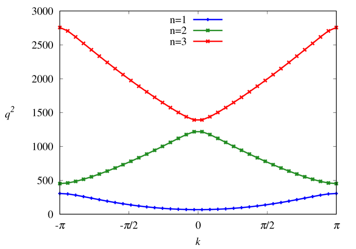
Figure 1: Squared momentum $q^{2}$ versus the Bloch vector $k$ for the first three bands. The data were obtained for a model with no disorder for $N=35$ wells separated by barriers of strength $U=15.0$.

In figure 2 we show a typical Bloch eigenfunction obtained for the same values of the parameters $N$ and $U$. The wavefunction $\Theta^{(q)}(\theta)$ has Bloch wavevector $k=0.428\pi$ which corresponds to a momentum $q\simeq 11.04$ and energy $q^{2}\simeq 121.9$ in the first band.

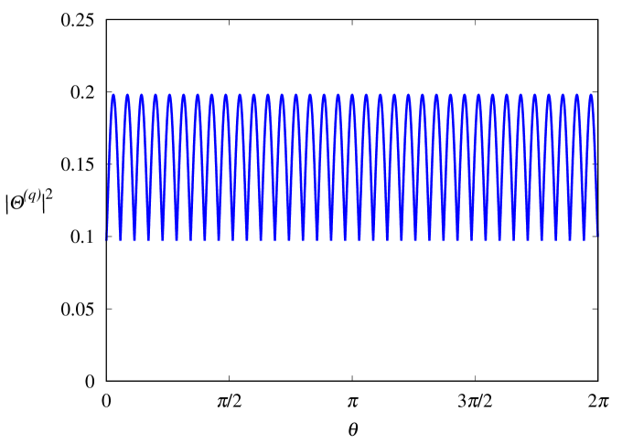
Figure 2: Squared modulus of the angular eigenfunction $\Theta^{(q)}(\theta)$ versus the angle variable $\theta$ for Bloch wavevector $k=0.428\pi$, which corresponds to $q\simeq 11.04$ (i.e. $q^{2}\simeq 121.9$). The data were obtained for a model with $N=35$ wells separated by barriers of strength $U=15.0$.

The wavefunction was normalised with the condition (17).

3.4 Infinite aperiodic Kronig-Penney model

To gain insight on the structure of the eigenstates of the model (8) when disorder is present, one can consider the corresponding infinite model, defined by the Schrödinger equation

$$-\frac{d^{2}\Theta}{dx^{2}}+\sum_{n=-\infty}^{\infty}U_{n}\delta\left(x-x_{n}\right)\Theta=q^{2}\Theta$$ (21)

with $x\in\mathbf{R}$. The delta barriers in the model (21) are centred at the random positions $\{x_{n}\}$, with $\langle x_{n}\rangle=n\alpha$. As is well known, the eigenstates of the infinite Kronig-Penney model (21) are localised. Their spatial extension is determined by the inverse localisation length, which can be defined in terms of the $\Theta_{n}=\Theta(x_{n})$ values as

$$\lambda=\lim_{N\to\infty}\frac{1}{N}\sum_{n=1}^{N}\ln\left|\frac{\Theta_{n+1}}{\Theta_{n}}\right|.$$ (22)

Note that the inverse localisation length (or Lyapunov exponent) (22) is a deterministic quantity due to its self-averaging property (see, e.g., [52]).

An analytical expression for the inverse localisation length (22) was derived for the case of weak disorder in [53, 54, 55]. As shown in [53], disorder can be considered weak provided that

$$\begin{array}[]{cccc}\langle u_{n}^{2}\rangle\ll U^{2},&\langle\Delta_{n}^{2}\rangle q^{2}\ll 1,&\mbox{ and }&\langle\Delta_{n}^{2}\rangle U\ll 1.\end{array}$$ (23)

If conditions (23) are met, one obtains

$$\begin{array}[]{ccl}\lambda&=&\displaystyle\frac{1}{8\alpha\sin^{2}k}\left[\frac{\sin^{2}(q\alpha)}{q^{2}}\langle u_{n}^{2}\rangle W_{1}(k)+U^{2}\langle\Delta_{n}^{2}\rangle W_{2}(k)\right.\\ &-&\displaystyle\left.2\left|\frac{\sin(q\alpha)}{q}\right|U\sqrt{\langle u_{n}^{2}\rangle\langle\Delta_{n}^{2}\rangle W_{1}(k)W_{2}(k)}\;\cos k\sin\left(2\eta\right)\right].\end{array}$$ (24)

The functions $W_{1}(k)$ and $W_{2}(k)$ in (24) are the Fourier transforms of the normalised binary correlators of the random variables $u_{n}$ and $\Delta_{n}$, i.e.,

$$\begin{array}[]{ccl}W_{1}\left(k\right)&=&\displaystyle 1+2\sum_{l=1}^{\infty}\frac{\langle u_{n}u_{n+l}\rangle}{\langle u_{n}^{2}\rangle}\cos(2kl)\\ W_{2}\left(k\right)&=&\displaystyle 1+2\sum_{l=1}^{\infty}\frac{\langle\Delta_{n}\Delta_{n+l}\rangle}{\langle\Delta_{n}^{2}\rangle}\cos(2kl).\\ \end{array}$$ (25)

The parameter $\eta$ in (24) determines the degree of cross-correlation of the $u_{n}$ and $\Delta_{n}$ variables. The values of $\eta$ range from $\eta=\pi/4$ (which corresponds to the extreme case of total positive cross-correlation) to $\eta=-\pi/4$ (total negative cross-correlation); for $\eta=0$ the cross-correlations vanish. For details on the effect of cross-correlations see Refs. [53, 56].

Expression (24) is a perturbative result, valid within the second-order approximation in the disorder strength. It shows that, within this approximation, the localisation length diverges in any energy interval over which the power spectra (25) vanish. This implies that an effective localisation-delocalisation transition can occur in the 1D Kronig-Penney model (21) provided that the disorder exhibits the specific long-range correlations which make the power spectra (25) vanish over a continuous energy range.

It is possible to construct sequences of self- and cross-correlated random variables $u_{n}$ and $\Delta_{n}$ such that the corresponding power spectra (25) vanish over pre-defined intervals. A way to produce such sequences was presented in [55]; for the sake of completeness, we outline the main steps in B.

As an application of the theory, we considered the Kronig-Penney model (21) with barriers of average strength $U=15.0$, disorder intensity $\sqrt{\langle\Delta_{n}^{2}\rangle}~{}=~{}0.007$ and $\sqrt{\langle u_{n}^{2}\rangle}=4.0$ and we compared the case of totally uncorrelated disorder with two cases of correlated disorder. We used disorder self-correlations to generate effective mobility edges by choosing compositional and structural disorders with identical power spectra of the form

$$W_{1}(k)=W_{2}(k)=\left\{\begin{array}[]{ccl}\displaystyle\frac{\pi}{2\left(k_{2}-k_{1}\right)}&\mbox{ if }&k\in\left[k_{1},k_{2}\right]\\ 0&\mbox{ if }&k\in\left[0,k_{1}\right]\cup\left[k_{2},\frac{\pi}{2}\right]\\ \end{array}\right.$$ (26)

and we considered two cases: in the first case we set the mobility edges at $k_{1}=0.46\pi$ and $k_{2}=0.5\pi$, while in the second case we selected the values $k_{1}=0.35\pi$ and $k_{2}=0.40\pi$. The first choice generates a single, wider, localisation window, while the second produces two narrower localisation windows. We analysed the cases of positive, absent, and negative cross-correlations; in the figures the respective cases are marked with the numbers (1), (2), and (3) and associated to the colours blue, green, and red in this section as well as in Secs. 3.5 and 3.6. Before proceeding, we would like to remark that we used power spectra of the form (26) in all the cases of correlated disorder which are numerically studied in this paper.

The Lyapunov exponent $\lambda$ for the infinite model (21) was obtained by numerically computing the right-hand side of (22). The results for the inverse localisation length are shown in figure 3 for the case of uncorrelated disorder and in figures 4 and 5 for the case of correlated disorder.

Figure 3: Inverse localisation length $\lambda$ versus energy $q^{2}$ for the first energy band. The data were obtained for uncorrelated disorder. The inset shows the corresponding localisation length.

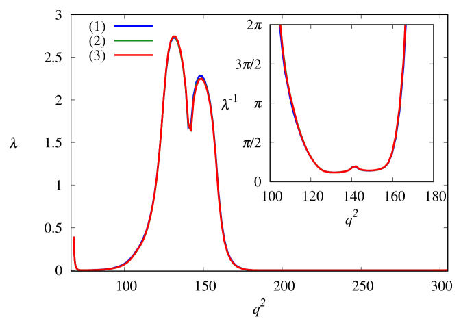
Figure 4: Inverse localisation length $\lambda$ versus energy $q^{2}$ for the first energy band. Self-correlations were used to produce a single localisation window. The blue solid line (1) corresponds to positive cross-correlations; the green line (2) and the red line (3) to absent and negative cross-correlations, respectively. The inset shows the corresponding localisation length.

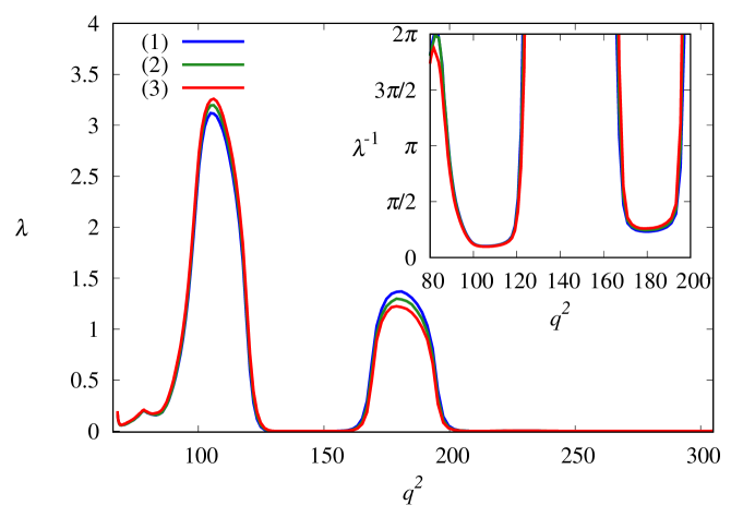
Figure 5: As in figure 4 but with different self-correlations so that two localisation windows were generated instead of one.

In the previous figures the energy covers the first allowed band and the inset shows the localisation length $l_{\mathrm{loc}}=\lambda^{-1}$. For the sake of clarity, in the case of correlated disorder we considered the localisation length only within the windows of enhanced localisation, excluding the rest of the energy band, where $l_{\mathrm{loc}}$ is many orders of magnitude larger than $2\pi$.

By comparing figure 3 with figures 4 and 5, one can see that correlations of the disorder have a twofold effect: they strongly enhance the localisation of the eigenstates within the selected energy windows and delocalise all the other eigenstates [57]. This enhancement of localisation turns out to be particularly relevant for the finite model we are interested in. In fact, the finite size of the domain of the angle variable implies that angular localisation needs to be sufficiently strong to be meaningful; at the same time, as discussed in Sec. 3.5, in our model structural disorder is necessarily weak because of built-in bounds, while compositional disorder is often also reduced by physical constraints of the experimental setup. The ingenious use of correlations to strengthen localisation, first suggested in [57], is therefore a crucial tool to produce angular localisation of the wavefunctions.

We also observe that in figure 4 the Lyapunov exponent drops in the middle of the localisation window. We interpret this decrease as a manifestation of the anomaly which appears when the Bloch wavevector takes the value $k=\pi/2$, as shown in [54]. It is known that correlations can enhance the anomaly in the Anderson model [58]; the numerical data suggest that similar effects occur in the Kronig-Penney model. As a final remark, we observe that cross-correlations do not change much the value of the Lyapunov exponent when self-correlations create a single localisation window. This is due to the position of the selected localisation window, which is centred around the Bloch vector $k=\pi/2$. As can be seen from (24), cross-correlations appear in the Lyapunov exponent through a term which is proportional to $\cos k$, and therefore their effect is reduced if the localisation window occurs for values of the Bloch vector which are close to $\pi/2$. Cross-correlations produce larger differences when localisation windows occupy different positions; as shown by figure 6(b), their effect is more evident in higher energy bands, as greater values of $q^{2}$ increase the relative weight of structural disorder with respect to the compositional one.

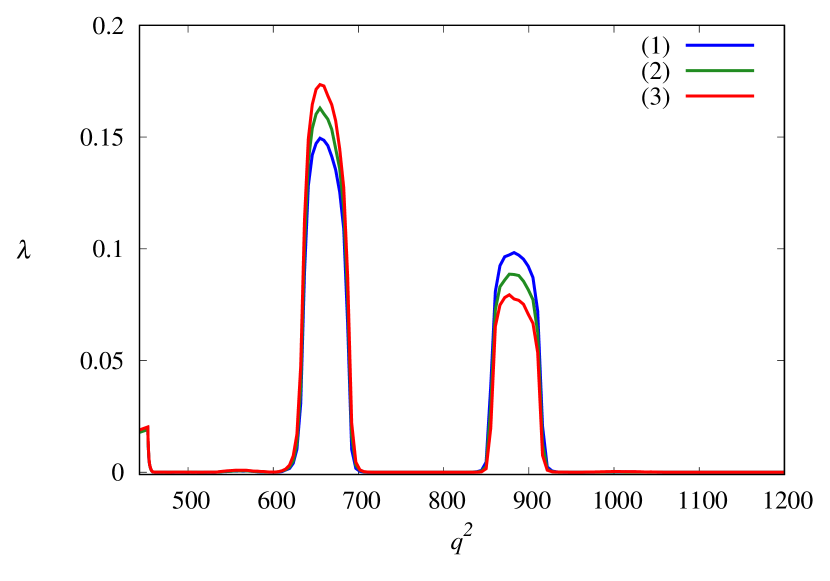
(a) Second energy band

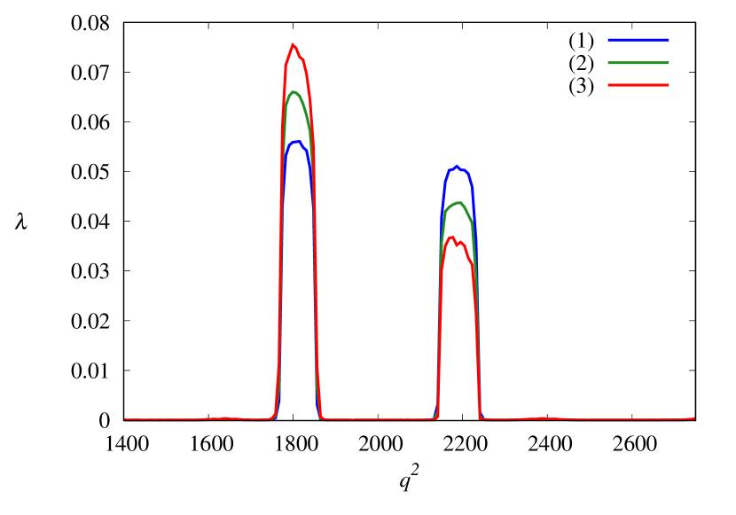
(b) Third energy band

Figure 6: Inverse localisation length $\lambda$ versus energy $q^{2}$ for the second and third energy bands. The same self-correlations used in figure 5 were also applied here

to produce two localisation windows. The blue solid line (1) corresponds to positive cross-correlation; the green line (2) and red line (3) to absent and negative cross-correlations, respectively.

3.5 Finite aperiodic Kronig-Penney model

Some caution is required when one tries to apply the results obtained for the infinite Kronig-Penney model (21) to the finite model (8). The fact that the angle variable is bounded within the $[0,2\pi]$ interval entails several differences between the two models. In the first place, one can speak of localised states for the model (8) only if their localisation length $l_{\mathrm{l}oc}$ is considerably less than the span of the angle variable, i.e., if

$$l_{\mathrm{l}oc}\ll 2\pi.$$ (27)

A second difference is that the finite size of the angle domain limits the number $N$ of barriers in model (8). As already noted, real radial barriers have a certain width and therefore $N$ cannot be arbitrarily large. In principle one could build very thin radial barriers; this would make possible to increase their number. This strategy, however, has a drawback: a higher number of barriers implies a smaller average angular spacing $\alpha=2\pi/N$ and, therefore, a weaker structural disorder. In fact, structural disorder cannot be so strong that a barrier might step over its nearest neighbours; increasing the number of barriers inevitably leads to barriers jumping each other even if disorder is weak. Barrier swaps can be prevented by confining the displacements $\Delta_{n}$ within the average disk slice allotted to each barrier; this sets the following upper bound on the variables $\Delta_{n}$:

$$\left|\Delta_{n}\right|\leq\frac{\alpha}{2}=\frac{\pi}{N}.$$ (28)

The constraint (28) shows that increasing the number of barriers necessarily reduces the strength of disorder and, therefore, the localisation of the angular wavefunction.

It is important to observe that the random displacements $\Delta_{n}$ may violate condition (28) if they are generated according to the recipe presented in B. In fact, the angular displacements $\Delta_{n}$ are obtained via sums of independent and identically distributed random variables with finite variance, as shown by (88); the central limit theorem therefore ensures that the $\Delta_{n}$ variables have a Gaussian distribution

$$p(\Delta_{n})=\frac{1}{\sqrt{2\pi\sigma_{\Delta}^{2}}}\exp\left(-\frac{\Delta_{n}^{2}}{2\sigma_{\Delta}^{2}}\right)$$ (29)

with $\sigma_{\Delta}=\sqrt{\langle\Delta_{n}^{2}\rangle}$ being the strength of the structural disorder. One can conclude that the probability that the $n$-th angular displacement violates the condition (28) is

$$\mathrm{Pr}\left(\left|\Delta_{n}\right|>\frac{\alpha}{2}\right)=1-\mathrm{erf}\left(\frac{\alpha}{2\sqrt{2}\sigma_{\Delta}}\right)$$ (30)

where $\mathrm{erf}(x)$ is the error function, defined as

$$\mathrm{erf}(x)=\frac{2}{\sqrt{\pi}}\int_{0}^{x}e^{-t^{2}}\mathrm{d}t.$$

For very weak disorder $\sigma_{\Delta}\ll\alpha$ and the probability (30) is exponentially small; for stronger structural disorder, however, the probability (30) ceases to be negligeable. In order to ensure that no violation of condition (28) occurs, one can discard the sequences of displacements in which one or more variables $\Delta_{n}$ fail to fulfil condition (28). Discarding whole sequences rather than individual displacements preserves intact the disorder correlations. In mathematical terms, one should “clip” the tails of the Gaussian distribution of each individual $\Delta_{n}$ variable in order to enforce condition (28). In this way, one considers variables $\Delta_{n}$ with distribution

$$\begin{array}[]{ccc}p(\Delta_{n})&=&\left\{\begin{array}[]{ccl}\displaystyle\mathcal{N}\exp\left(-\frac{\Delta_{n}^{2}}{2\sigma_{0}^{2}}\right)&\mbox{ for}&\displaystyle\Delta_{n}\in\left[-\frac{\alpha}{2},\frac{\alpha}{2}\right]\\ 0&\mbox{ for }&\displaystyle\Delta_{n}\notin\left[-\frac{\alpha}{2},\frac{\alpha}{2}\right]\\ \end{array}\right.\end{array}$$ (31)

where $\mathcal{N}$ is a normalisation constant. Note that the parameter $\sigma_{0}^{2}$ of the distribution (31) and the variance of the disorder $\sigma_{\Delta}^{2}$ are linked by the relation

$$\sigma^{2}_{\Delta}=\sigma_{0}^{2}\left[1-\frac{\alpha}{\sqrt{2\pi}\sigma_{0}}\frac{\displaystyle\exp\left(-\frac{\alpha^{2}}{8\sigma_{0}^{2}}\right)}{\displaystyle\mathrm{erf}\left(\frac{\alpha}{\sqrt{8}\sigma_{0}}\right)}\right].$$

The geometry of the problem subjects the sequences $\{\Delta_{n}\}$ of angular displacements to an additional constraint which does not exist in the infinite model (21). If the origin is set in correspondence with the first barrier, $\theta_{1}=0$, from Eqs. (7) and (13) one obtains that the position of the $n$-th barrier is

$$\begin{array}[]{ccc}\displaystyle\theta_{n}=\alpha(n-1)+\sum_{k=1}^{n-1}\Delta_{k}&\mbox{ for }&n=2,3,\ldots,N.\end{array}$$

In particular, the position of the last barrier is

$$\theta_{N}=2\pi\frac{N-1}{N}+\sum_{k=1}^{N-1}\Delta_{k}.$$

Due to the circular nature of the problem, the $N$-th barrier cannot be placed after the first barrier, i.e., one must have

$$\theta_{N}<2\pi.$$

The variables (13) must therefore satisfy the additional condition

$$\sum_{k=1}^{N-1}\Delta_{k}\leq\frac{2\pi}{N}.$$ (32)

Considering weak disorder reduces but does not eliminate the possibility of a violation of the condition (32). In numerical simulations we resorted to “weeding out” the sequences $\{\Delta_{n}\}$ for which the criterion (32) was not respected. This introduces another difference in the statistical properties of the variables (13) for the finite model (8) with respect to the infinite system (21).

To ascertain whether, in spite of these differences, the localisation behaviour of the eigenstates of the infinite model (21) is preserved in the finite model (8), we numerically studied the structure of the eigenstates of the latter. To determine the eigenstates of the model (8), we wrote the system (15) of linear equations in matrix form:

$$\mathbf{M}(q)\left(\begin{array}[]{c}\Theta_{1}\\ \vdots\\ \Theta_{N}\\ \end{array}\right)=\left(\begin{array}[]{c}0\\ \vdots\\ 0\\ \end{array}\right)$$ (33)

where $\mathbf{M}(q)$ is the cyclic tridiagonal matrix

$$\mathbf{M}(q)=\left(\begin{array}[]{ccccccccccc}\varepsilon_{1}&\gamma_{2}&0&\cdots&\cdots&\cdots&\cdots&\cdots&\cdots&0&\gamma_{1}\\ \gamma_{2}&\varepsilon_{2}&\gamma_{3}&0&\cdots&\cdots&\cdots&\cdots&\cdots&\cdots&0\\ 0&\gamma_{3}&\varepsilon_{3}&\gamma_{4}&0&\cdots&\cdots&\cdots&\cdots&\cdots&0\\ \vdots&\ddots&\ddots&\ddots&\ddots&\ddots&&&&&\vdots\\ \vdots&&\ddots&\ddots&\ddots&\ddots&\ddots&&&&\vdots\\ \vdots&&&0&\gamma_{n+1}&\varepsilon_{n}&\gamma_{n+1}&0&&&\vdots\\ \vdots&&&&\ddots&\ddots&\ddots&\ddots&\ddots&&\vdots\\ \vdots&&&&&\ddots&\ddots&\ddots&\ddots&\ddots&\vdots\\ 0&\cdots&\cdots&\cdots&\cdots&\cdots&0&\gamma_{N-2}&\varepsilon_{N-2}&\gamma_{N-1}&0\\ 0&\cdots&\cdots&\cdots&\cdots&\cdots&\cdots&0&\gamma_{N-1}&\varepsilon_{N-1}&\gamma_{N}\\ \gamma_{1}&0&\cdots&\cdots&\cdots&\cdots&\cdots&\cdots&0&\gamma_{N}&\varepsilon_{N}\\ \end{array}\right).$$ (34)

We let the momentum $q$ vary within the allowed bands and we determined the values of $q$ for which a non-vanishing solution $\{\Theta_{n}^{(q)}\}$ of the system (33) exists. More specifically, for each value of $q$ we numerically diagonalised the matrix (34), computing the eigenvalues $\{\mu_{k}(q)\}$ and the corresponding eigenvectors $\{\Theta^{(q)}(k)\}$ (with $k=1,\ldots,N$). We used these results to evaluate the “density of states”

$$\rho=-\frac{1}{\pi}\sum_{k=1}^{N}\mathrm{Im}\frac{1}{\mu^{(q)}(k)+i\varepsilon}.$$

For each value of $q$ such that $\rho=O\left(1/\varepsilon\right)$, we identified the eigenstate $\Theta^{(q)}(\overline{k})$ with the smallest eigenvalue $\mu_{\overline{k}}(q)$ (in absolute value) as a solution of the homogenous system (33). In this way we obtained the eigenstates of the tight-binding system (15) and, via (16), the eigenfunctions of the disordered Kronig-Penney model (8). We then proceeded to analyse the localisation properties of both models making use of the inverse participation ratio (IPR) to evaluate the spatial extension of the discrete eigenvectors of the tight-binding model (15) and of the continuous eigenstates of the finite Kronig-Penney model (8). As a further check, we also computed the entropic localisation length of the eigenvectors of the tight-binding model (15).

The participation ratio $P^{-1}(q)$ represents a commonly used measure of the portion of space where an eigenstate significantly differs from zero [5, 59]. For the discrete model (15) we defined the IPR using the relation

$$P(q)=\frac{N}{2\pi}\sum_{n=1}^{N}\left|\Theta_{n}^{(q)}\right|^{4},$$ (35)

with the vectors $\{\Theta_{n}^{(q)}\}$ normalised according to (18). We chose the prefactor in (35) so that $P^{-1}=2\pi$ for an extended state. We used the definition

$$P(q)=\int_{0}^{2\pi}\left|\Theta^{(q)}(\theta)\right|^{4}\mathrm{d}\theta$$ (36)

for the eigenstates of the continuous model (8) normalised with the condition (17).

The entropic localisation length was first applied in [60, 61, 62] to quantum chaos problems and represents a measure of the effective number of components of eigenvectors. After normalising the eigenvectors $\{\Theta^{(q)}_{n}\}$ with the condition (18), we computed the corresponding information entropy

$$S_{N}(q)=-\sum_{n=1}^{N}|\Theta_{n}^{(q)}|^{2}\ln|\Theta_{n}^{(q)}|^{2}$$ (37)

from which we obtained the entropic localisation length, defined as

$$l_{e}(q)=\frac{2\pi}{N}\exp\left[S_{N}\left(q\right)\right].$$ (38)

As in the previous case, the normalisation factor of the entropic localisation length (38) was chosen so that, for the extended Bloch waves (19), $l_{e}=2\pi$.

We observe that both the entropic localisation length $l_{e}$ and the inverse participation ratio $P$ are functions of random eigenvectors and, as such, are random variables themselves whose values fluctuate from one disorder realisation to the next. This sets another difference between the finite models (8) and (15) and their infinite counterpart (21), which is endowed with a self-averaging inverse localisation length. To gain insight on the statistical properties of the entropic localisation length and of the IPR, we considered the average value and the standard deviation of both parameters. We defined the average entropic localisation length as

$$\langle l_{e}(q)\rangle=\frac{1}{N_{r}}\sum_{n=1}^{N_{r}}l_{e}^{(n)}(q)$$ (39)

where $N_{r}$ is the total number of disorder realisations and $l_{e}^{(n)}(q)$ is the value of $l_{e}(q)$ obtained in the $n$-th realisation. When performing the ensemble average (39), one should also consider that the eigenvalues of the momentum $q$ suffer slight shifts from one disorder realisation to the next. For this reason we obtained $\langle l_{e}\rangle$ by dividing the energy band in 100 intervals and by constructing a histogram for $l_{e}(q)$. In the case of the inverse participation ratio, we computed its ensemble average

$$\langle P(q)\rangle=\frac{1}{N_{r}}\sum_{n=1}^{N_{r}}P^{(n)}(q)$$ (40)

and then we plotted the inverse $\langle P\rangle^{-1}$.

As observed in [63], (39) is not the only meaningful way to define an average entropic localisation length. One could also consider the alternative form

$$\overline{l_{e}(q)}=\frac{2\pi}{N}\exp\left[\langle S_{N}(q)\rangle\right]$$ (41)

with

$$\langle S_{N}(q)\rangle=\frac{1}{N_{r}}\sum_{n=1}^{N_{r}}S_{N}^{(n)}(q).$$

Our numerical data, however, showed that in the present problem formulae (39) and (41) produce strikingly similar results, the main difference being that the entropic localisation length defined by (41) usually turns out to be a few percents shorter than its counterpart (39), in agreement with the results found in [63].

In our numerical studies, we considered the angular Kronig-Penney model (8) and its tight-binding homologue (15) with $N=35$ barriers and the same disorder parameters used for their infinite counterpart in Sec. 3.4, i.e., average barrier strength $U=15.0$, compositional and structural disorders with respective intensities $\sqrt{\langle u_{n}^{2}\rangle}=4.0$ and $\sqrt{\langle\Delta_{n}^{2}\rangle}=0.007$. As in Sec. 3.4, we considered two cases: in the first one we generated a single localisation window by setting effective mobility edges with Bloch vectors $k_{1}=0.46\pi$ and $k_{2}=0.5\pi$. In the second case we selected the values $k_{1}=0.35\pi$ and $k_{2}=0.40\pi$ and we thus obtained two localisation windows. We considered positive, absent and negative cross-correlations; as noted before, in the figures the respective cases are labelled with the numbers (1), (2), and (3) and associated to the colours blue, green, and red. In all cases the averages were computed over an ensemble of $N_{r}=1000$ disorder realisations. We present our numerical data for the average value of the entropic localisation length $\langle l_{e}\rangle$ in the top panels of figure 7; the inverse of the average of the IPR $\langle P\rangle^{-1}$ is shown in the middle panels of figure 7 for the tight-binding model (15) and in the bottom panels for the Kronig-Penney model (8).

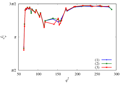
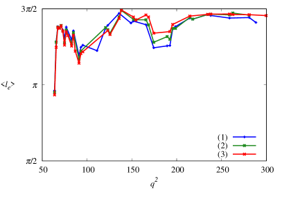
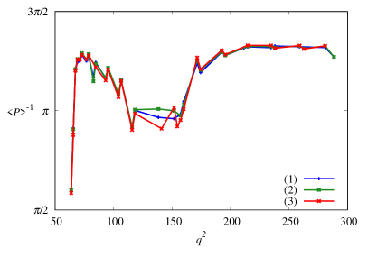
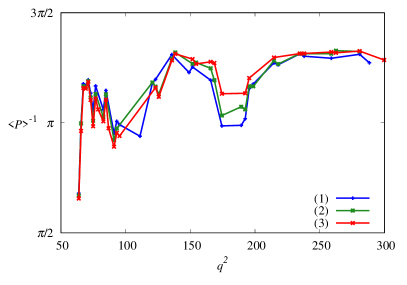
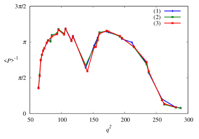
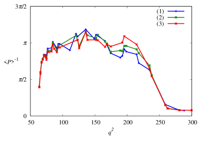
Figure 7: Average entropic localisation length and IPR computed over an ensemble of $N_{r}=1000$ disorder configurations, for the case $U=15.0$, $\sqrt{\langle u_{n}^{2}\rangle}=4.0$ and $\sqrt{\langle\Delta_{n}^{2}\rangle}=0.007$. Top panels: average entropic localisation length $\langle l_{e}\rangle$ versus energy $q^{2}$. Middle panels: Inverse of the average IPR $\langle P\rangle^{-1}$ versus energy $q^{2}$ for the discrete model (15). Bottom panels: inverse of the average IPR $\langle P\rangle^{-1}$ versus energy $q^{2}$ for the continuous model (8). Left panels: one localisation window ($k_{1}=0.46\pi$ and $k_{2}=0.5\pi$). Right panels: two localisation windows ($k_{1}=0.35\pi$ and $k_{2}=0.40\pi$).

When dealing with the entropic localisation length (38) and the inverse participation ratio (35), one should keep in mind that the average values (39) and (40) do not provide a complete picture of the behaviour of the eigenstates of the Kronig-Penney model (8). This is due to the fact that both localisation lengths exhibit very strong fluctuations from one disorder realisation to the next. In our numerical study, for example, we found that the typical values of the standard deviation of $l_{e}$ and $P^{-1}$ varied between $\pi$ and $2\pi$. We did not represent the corresponding error bars in figure 7 because they were too large and significantly reduced the clarity of the data. Even more important, increasing the number of disorder realisations did not produce a diminution of the standard deviation. The observed statistical behaviour of the two generalised localisation lengths agrees with the properties described in the literature [63, 64, 4].

The strong fluctuations of $l_{e}$ and $P^{-1}$ can be exploited in the construction of an experimental setup designed to obtain a robust localisation enhancement. In fact, one can select a specific disorder realisation which produces a particularly strong localisation of the angular eigenstates in the selected energy interval: this is illustrated in the panels of figure 8 which represent the entropic localisation length and the IPR for such a single realisation of the disorder.

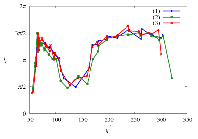
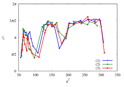
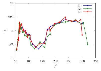
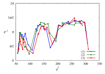
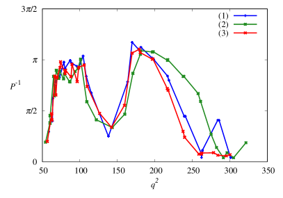
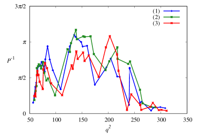
Figure 8: As figure 7 but for a specific disorder realisation.

The numerical results displayed in the figures of this section clearly show that correlated disorder can produce a significative enhancement of localisation in predefined energy windows, although the magnitude of the effect fluctuates considerably over the ensemble of disorder realisation. We conclude that the effects of disorder correlations survive (albeit in an attenuated form) in the tight-binding model (15) and in the finite Kronig-Penney model (8), in spite of the limitations imposed by the finite size and by the geometry of the system.

As a further illustration of the particularly strong localisation that can be achieved in specific realisations of the disorder, in figure 9 we show the most localised eigenfunction of the Kronig-Penney model (8) obtained with the same disorder realisation represented in figure 8. Specifically, we considered the eigenfunction with momentum $q\simeq 11.045$ and energy $q^{2}\simeq 122.0$ in the first energy band.

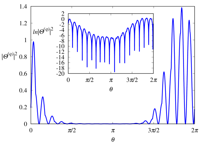
Figure 9: Squared modulus of the angular eigenfunction $\Theta^{(q)}(\theta)$ versus the angle variable $\theta$ with momentum $q\simeq 11.04$ and energy $q^{2}\simeq 122.0$, for the same disorder realisation as in figure 8.

The eigenfunction was derived for the case in which structural and compositional disorder are self-correlated but not cross-correlated. The energy of this eigenfunction is the closest within the perturbed spectrum to the energy of the Bloch wave considered in Sec. 3.4. We can consider the wavefunction represented in figure 9 as the counterpart of the wavefunction pictured in figure 2. Comparing the two figures, it is easy to see that correlated disorder manages to produce a rather good localisation of specific waves.

3.6 Resonance effects in the continuous Kronig-Penney model

So far, in our analysis of the localisation properties of the Kronig-Penney model (8) we have relied on the close relationship which exists between the model itself and its tight-binding counterpart (15). In particular, we have used the correspondence between the continuous eigenfunctions $\Theta(\theta)$ of the former and the discrete eigenvectors $\left\{\Theta_{n}\right\}$ of the latter. This correspondence, established in Sec. 3.2, is corroborated by the numerical data presented in Sec. 3.5, which reveal the roughly parallel behaviour of the IPR of the eigenstates of the models (8) and (15). However, a careful comparison of the middle panels with the bottom panels of figure 7 and 8 also shows that the IPR’s of the two models behave differently in the higher part of the energy band. When the energy approaches the top of the band, the participation ratio of the tight-binding model (15) keeps high values, indicating that the discrete eigenstates $\{\Theta_{n}\}$ are extended, whereas the participation ratio for the Kronig-Penney model (8) falls close to zero in the same energy range, a sign that the spatial extension of the continuous eigenstates $\Theta(\theta)$ is strongly reduced. This discrepancy can be explained as a manifestation of resonance effects occurring in the Kronig-Penney model (8) and shows that, under specific circumstances, the correspondence between this model and its tight-binding homologue (15) breaks down.

To understand this point, let us consider an eigenvector $\left\{\Theta_{n}\right\}$ of the tight-binding model (15) with momentum $q$. Let us suppose that structural disorder produces a displacement of the $n$-th and $(n+1)$-th radial barriers such that

$$q\left(\theta_{n+1}-\theta_{n}\right)=\pi+\varepsilon$$ (42)

with $\varepsilon\to 0$. For the sake of simplicity, we will assume that only the $n$-th well satisfies a resonance condition of the form (42). Substituting the identity (42) in (16), one obtains that the eigenstate of the Kronig-Penney model (8) with momentum $q$ is equal to

$$\Theta(\theta)=\left\{\begin{array}[]{lcl}\displaystyle\mathcal{N}\left[\frac{\Theta_{n+1}-\Theta_{n}}{\varepsilon}\sin\left[q\left(\theta-\theta_{n}\right)\right]+O\left(\varepsilon^{0}\right)\right]&\mbox{ if }&\theta\in\left[\theta_{n},\theta_{n+1}\right]\\ O\left(\varepsilon^{0}\right)&\mbox{ if }&\theta\notin\left[\theta_{n},\theta_{n+1}\right]\end{array}\right.$$ (43)

The constant $\mathcal{N}$ can be derived from the normalisation condition (17); one has

$$\mathcal{N}=\sqrt{\frac{2q}{\pi}}\frac{\varepsilon}{\Theta_{n+1}-\Theta_{n}}\left[1+O\left(\varepsilon^{2}\right)\right].$$

Substituting this expression in (43) one obtains that the resonant eigenstate has the form

$$\Theta(\theta)=\left\{\begin{array}[]{lcl}\displaystyle\sqrt{\frac{2q}{\pi}}\sin\left[q\left(\theta-\theta_{n}\right)\right]+O\left(\varepsilon\right)&\mbox{ if }&\theta\in\left[\theta_{n},\theta_{n+1}\right]\\ O\left(\varepsilon\right)&\mbox{ if }&\theta\notin\left[\theta_{n},\theta_{n+1}\right]\end{array}\right.$$ (44)

(44) shows that, when the phase of the eigenfunction increases by an integer multiple of $\pi$ in a potential well, the mode becomes locked in that well. In other words, the well acts as a Fabry-Pérot resonator.

In this case, there is a profound difference between the eigenvectors of the tight-binding model (15) and the eigenstates of the continuous Kronig-Penney model (8). The discrete eigenvectors $\{\Theta_{n}\}$ have non-vanishing components in the whole $[0,2\pi]$ range, whereas the continuous eigenfunctions $\Theta(\theta)$ are significantly different from zero only in a single well. When this happens the continuous eigenfunctions $\Theta(\theta)$ are much more localised than the corresponding eigenvectors $\left\{\Theta_{n}\right\}$; however, their reduced spatial extension must be counted as a resonance effect, and not as a true Anderson localisation. One might say that, in some sense, the eigenvectors of the tight-binding model (15) offer a better insight on the true localisation properties of the Kronig-Penney model (8) than the eigenfunctions of the model themselves.

Whether the resonance condition (42) is met or not determines if resonance effects cooperate with Anderson localisation in shaping the eigenfunctions of the Kronig-Penney model (8). As an example, let us consider once more the case of a Kronig-Penney model with $N=35$ barriers, mean field strength $U=15.0$ and compositional and structural disorders with strengths $\sqrt{\langle u_{n}^{2}\rangle}=4.0$ and $\sigma_{\Delta}=\sqrt{\langle\Delta_{n}^{2}\rangle}=0.007$. In this case the momentum $q$ takes values within the interval $q\in[q_{\mathrm{min}},q_{\mathrm{max}}]$ with $q_{\mathrm{min}}\simeq 8.2$ and $q_{\mathrm{max}}\simeq 17.5$ for the first band. The threshold value of the momentum for the onset of a Fabry-Pérot resonance is

$$q_{c}\simeq\frac{\pi}{\Delta\theta_{\mathrm{max}}}$$

where $\Delta\theta_{\mathrm{max}}$ is the largest angular distance between two consecutive barriers. In the absence of disorder, one has $\Delta\theta_{\mathrm{max}}=\alpha=2\pi/N$ and therefore

$$q_{c}=\frac{\pi}{\alpha}=\frac{N}{2}=17.5.$$ (45)

This shows that the threshold value of the momentum lies right at the top of the first band and, consequently, resonances are a marginal phenomenon in the first band of the periodic Kronig-Penney model.

Things are different when disorder is added, though. In our case $\sigma_{\Delta}~{}\ll~{}\alpha$ and the difference between the distributions (29) and (31) is irrelevant. Assuming that each barrier can swing up to $\pm 2\sigma_{\Delta}$ from its unperturbed position, one can conclude that the variation of the angular distance $\Delta\theta_{n}$ lies in the interval $[\alpha-4\sigma_{\Delta},\alpha+4\sigma_{\Delta}]$ and that in most cases one has

$$\alpha-3\sigma_{\Delta}\lesssim\Delta\theta_{n}\lesssim\alpha+3\sigma_{\Delta}.$$

This gives a critical value of the momentum

$$q_{c}\simeq\frac{\pi}{\alpha+3\sigma_{\Delta}}\simeq 15.66$$ (46)

which is considerably lower than the value (45) obtained in the absence of disorder. The value (46) corresponds to a critical energy $q_{c}^{2}\simeq 245.5$ which lies well within the first band and broadly agrees with the observed inflection point where the participation ratio for the Kronig-Penney model (8) starts to decline, see bottom panels of figure 7.

Note that, for resonant states of the form (43), the IPR (36) takes the value

$$P_{\mathrm{res}}(q)=\frac{3q}{2\pi}+O(\varepsilon),$$

which corresponds to a spatial extension

$$P_{\mathrm{res}}^{-1}(q)=\frac{2\pi}{3q}+O(\varepsilon).$$ (47)

We observe that strong resonances which confine the wavefunction to a single well do not occur for every disorder realisation, therefore (47) represents a lower bound for the average participation ratio. With the values of the parameters considered in numerical simulations, we can expect the parameter (47) to take values $P^{-1}_{\mathrm{res}}\simeq 0.12$ to 0.13 for $q$ ranging from 15.6 to 17.5. This is consistent with the asymptotic value $\langle P\rangle^{-1}\simeq 0.25$ of the average participation ratio obtained in numerical simulation at the top of the band. In conclusion, with the present values of the parameters one can expect the Anderson localisation to be the relevant phenomenon for energies at the bottom and in the wide middle of the first band, while resonant states become a dominant feature in the top fringe of the energy band.

The hypothesis that Fabry-Pérot resonances are the origin of the drastic reduction of the spatial extension of the wavefunctions of the Kronig-Penney model (8) is further confirmed by the fact that, if compositional disorder is strengthened, the critical threshold for the onset of resonant state is lowered. A stronger structural disorder extends the variation range of the angular width of the wells; as a consequence, lower values of $q$ are required to fullfill the resonance condition (42). Therefore the drop of the participation ratio should occur at lower energies than is the case for weaker structural disorder. This is in fact what happens, as can be seen in figure 10, which represents the inverse of the average IPR as in the bottom panels of figure 7 but for a Kronig-Penney model with stronger structural disorder, i.e., $\sigma_{\Delta}=0.021$, which is three times the strength of the previous case; the other parameters of the model were left unchanged.

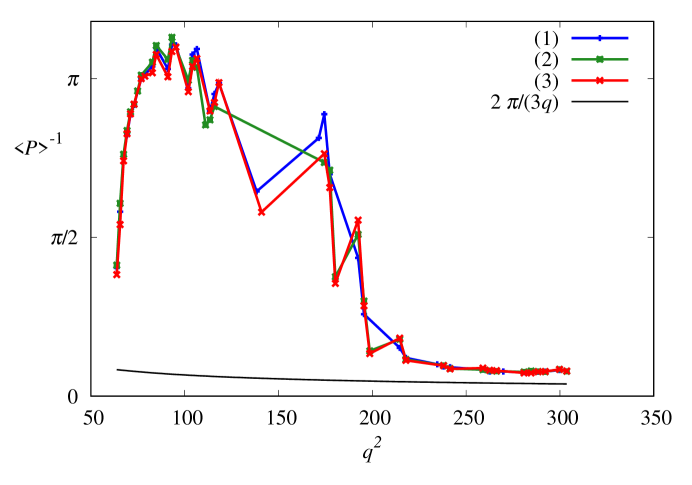
Figure 10: Inverse of the average IPR $\langle P\rangle^{-1}$ versus energy $q^{2}$ for the first energy band. The structural disorder strength is $\sigma_{\Delta}=0.21$. The black continuous line represents the limit behaviour given by (47).

To conclude this section, we remark that resonances have usually been neglected in the study of the infinite Kronig-Penney model (21). It might be worthwhile to check whether the interplay of localisation and resonance also play a role in that model.

3.7 Radial part of the Schrödinger equation

We now turn our attention to the radial part of the wavefunction. The solutions of (9) are linear combinations of independent Bessel functions of the first and second kind

$$R_{q}(r)=c_{1}J_{q}(\sqrt{E}r)+c_{2}Y_{q}(\sqrt{E}r).$$

If the particle is confined within the annulus, the wavefunction must vanish on the inner and outer circles of radii $r_{1}$ and $r_{2}$. Imposing the boundary conditions

$$R_{q}(\sqrt{E}r_{1})=R_{q}(\sqrt{E}r_{2})=0$$

leads to the solution

$$R_{q}(r)=\mathcal{N}\left[Y_{q}(\sqrt{E}r_{1})J_{q}(\sqrt{E}r)-J_{q}(\sqrt{E}r_{1})Y_{q}(\sqrt{E}r)\right],$$

where $\mathcal{N}$ is a normalisation constant, to be determined with the condition

$$\int_{r_{1}}^{r_{2}}\left|R_{q}(r)\right|^{2}r\mathrm{d}r=1,$$

while the values of the energy $E$ can be obtained by solving the equation

$$Y_{q}(\sqrt{E}r_{1})J_{q}(\sqrt{E}r_{2})-J_{q}(\sqrt{E}r_{1})Y_{q}(\sqrt{E}r_{2})=0.$$ (48)

It is convenient to rewrite (48) in the form

$$Y_{q}(x)J_{q}(\varkappa x)-J_{q}(x)Y_{q}(\varkappa x)=0$$ (49)

with $x=r_{1}\sqrt{E}$ and $\varkappa=r_{2}/r_{1}$. For any eigenvalue of the momentum $q$, let $x(q,s)$ be the $s$-th zero of the cross-product of Bessel functions (49), with $|x(q,s=1)|\leq|x(q,s=2)|\leq\ldots$ Then the eigenvalues of the total energy of the system can be labelled with the quantum numbers $(q,s)$ and take the form

$$E_{q,s}=\left(\frac{x(q,s)}{r_{1}}\right)^{2}.$$

On the other hand, for weak disorder each value $q$ of the angular quantum number can be written as a function of the Bloch wavenumber $k$ and of a band index $n$; it is therefore convenient to write the energy in the form

$$E(k,n,s)=\left(\frac{x[q(k,n),s]}{r_{1}}\right)^{2}.$$ (50)

The values $x(q,s)$ can be obtained by solving numerically (49); for larger values of $s$ one can also use the asymptotic expansion provided by the McMahon formula [65].

In figure 11 we plot the energy levels (50) as a function of the Bloch wavenumber $k$ for the values $n=1,2$ of the band index and $s=1,2$ of the radial quantum number. The data were obtained for $r_{1}=10\,\mbox{cm}$ and $r_{2}=25\,\mbox{cm}$ and for $U=15.0$. (The values of $r_{1}$ and $r_{2}$ correspond to the inner and outer radii of the cavity discussed in A.) The computation of the values of $q$ was done in the limit of vanishing disorder.

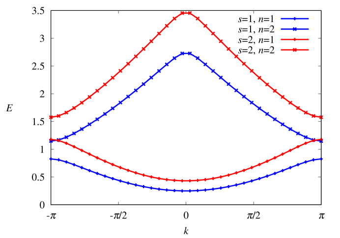
Figure 11: Energy levels $E(k,n,s)$ versus $k$ for $n=1,2$ and $s=1,2$. The energy values are measured in $\mbox{cm}^{-2}$.

Figure 11 shows that a good deal of overlapping can occur between energy bands with the same index $n$ but different radial numbers $s$. This implies that one can localise eigenstates with different radial numbers within a single window of the energy $E$ of the 2D model (1). This is what is shown in figure 12 which represents the behaviour of the participation ratio $P^{-1}$ as a function of the total energy $E$ (and not of the squared momentum $q^{2}$, as was done in Secs. 3.5 and 3.6). The data correspond to the single disorder realisation shown in figure 8 for the case of self-correlated disorder without cross-correlations.

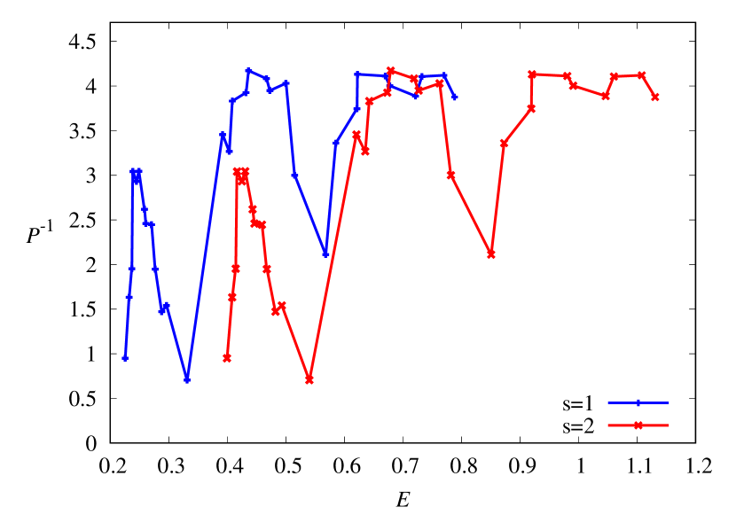
(a) Tight-binding model (15)

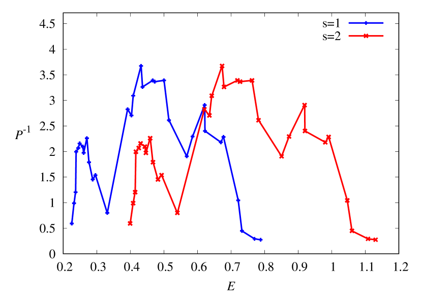
(b) Kronig-Penney model (21)

Figure 12: Inverse of the IPR $P^{-1}$ versus energy $E$ (in $\mbox{cm}^{-2}$) for the discrete model (15) and for the continuous model (21) for the first two bands, $s=1$ and $s=2$. The data correspond to the single disorder configuration shown in figure 8.

We would like to stress that the localisation within the same energy window of states with different angular quantum numbers is a genuine manifestation of the two-dimensional nature of the model (1).

To conclude this section, in figure 13 we show a graphical representation of the disorder-induced localisation of the complete wavefunctions. We consider the wavefunctions with quantum numbers $q\simeq 11.04$ and $s=1,2,3$; we show the extended wavefunctions in the subfigures on the left and their localised counterparts in the right subfigures. The figure 13 complements the information for the angular part of the wavefunction provided by figures 2 and 9 with the information relative to the radial part. The wavefunctions in the three figures differ for the values of the radial wavenumber $s$. Note that $s$ is equal to the number of nodes of the radial part of the wavefunction; therefore the square modulus of the wavefunction has $s$ circular ridges, whose height decreases for increasing values of the radial coordinate.

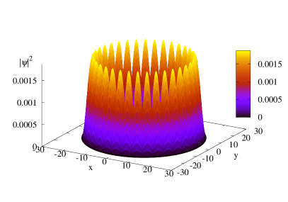
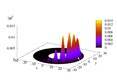
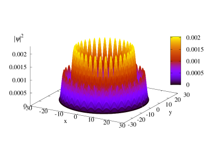
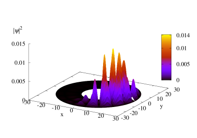
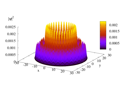
Figure 13: Squared modulus $|\psi_{q,s}|^{2}$ of the wavefunction with quantum numbers $q\simeq 11.04$ and (from top to bottom): $s=1,2,3$. Left panels: ordered system. Right panels: correlated disordered system.

4 Disorder with radial symmetry

In this section we investigate the second model, with disorder that depends on the radial coordinate. This part of the paper is focused on a different 2D problem, namely, a quantum particle moving on a plane under the influence of a central random potential.

4.1 Model with radius-dependent disorder

For a central random potential $U(r,\theta)=U(r)$ the stationary Schrödinger equation (1) is given by

$$\left[-\nabla^{2}+U(r)\right]\psi(r,\theta)=E\psi(r,\theta)$$ (51)

where $\nabla^{2}$ is the 2D Laplacian (2). Specifically, we consider a potential of the form

$$U(r)=\sum_{n=1}^{N}U_{n}\delta\left(r-r_{n}\right).$$ (52)

We assume that both the positions and the strengths of the $\delta$-barriers are random variables; the strengths $U_{n}$ are defined by (6) with mean value $U=\langle U_{n}\rangle$ as in the previous model, while the radial positions are given by

$$r_{n}=r_{1}+a(n-1)+a_{n}.$$ (53)

In (53), $a$ represents the average radial distance between two neighbouring barriers, while $a_{n}$ is the random radial displacement of the $n$-th barrier from its “lattice” position $r_{n}^{(0)}=r_{1}+a(n-1)$. Is it assumed that all $r_{n}>0$. We consider the case of weak disorder, defined by the conditions

$$\begin{array}[]{cccc}\langle u_{n}^{2}\rangle\ll U^{2},&\langle\Delta_{n}^{2}\rangle E\ll 1,&\mbox{ and }&\langle\Delta_{n}^{2}\rangle U\ll 1,\end{array}$$ (54)

which coincide with those set by (23) with the substitution $q^{2}\to E$ and where the symbol $\Delta_{n}$ now stands for

$$\Delta_{n}=a_{n+1}-a_{n}.$$

After separating the radial and the angular variables via (3), one obtains that the two parts of the wavefunction obey the equations

$$\frac{d^{2}\Theta}{d\theta^{2}}+l^{2}\Theta=0$$ (55)

and

$$\frac{d^{2}R}{dr^{2}}+\frac{1}{r}\frac{dR}{dr}+\left[E-\sum_{n=1}^{N}U_{n}\delta(r-r_{n})-\frac{l^{2}}{r^{2}}\right]R=0.$$ (56)

(55) has solutions

$$\Theta_{l}(\theta)=\frac{1}{\sqrt{2\pi}}e^{il\theta}$$

with $l$ integer. The functions $\Theta_{l}(\theta)$ are eigenfunctions of the angular momentum $L=-i\partial/\partial\theta$, which commutes with the Hamiltonian because of the circular symmetry of the model.

We are interested in two different but related problems: the localisation of the quantum states in the model (56) with an infinite number of circular barriers ($N\to\infty$) and the transmission properties of a random annulus with a finite number of barriers. To analyse these problems we first discuss in Sec. 4.2 under what circumstances a 2D model with circular symmetry can be reduced to its 1D counterpart. We then consider the localisation and transmission properties in Secs. 4.3 and 4.4.

4.2 The 2D Kronig-Penney model and its 1D analogue

When $N\to\infty$, the model defined by (56) represents a 2D variant of the 1D Kronig-Penney model (21), with Schrödinger equation

$$\frac{d^{2}R}{dr^{2}}+\frac{1}{r}\frac{dR}{dr}+\left[E-\sum_{n=1}^{\infty}U_{n}\delta(r-r_{n})-\frac{l^{2}}{r^{2}}\right]R=0.$$ (57)

The analogy with the 1D model (21) is easier to see if the radial wavefunction is expressed as

$$R(r)=\frac{X(r)}{\sqrt{r}}.$$

(57) can then be written in the new form

$$\frac{d^{2}X}{dr^{2}}+\left[E-\sum_{n=1}^{\infty}U_{n}\delta(r-r_{n})-\frac{l^{2}-1/4}{r^{2}}\right]X=0.$$ (58)

Replacing the symbol $r$ for the radial coordinate with $t$ allows one to interpret (58) as the equation of motion of a classical dynamical system

$$\ddot{X}+\left[E-\sum_{n=1}^{\infty}U_{n}\delta(t-t_{n})-\frac{l^{2}-1/4}{t^{2}}\right]X=0.$$ (59)

More specifically, (59) describes the dynamics of a parametric oscillator whose frequency varies in time under the influence of two different terms: a deterministic term, due to the centrifugal potential, which lowers the frequency and tends to vanish over long time scales, and a stochastic term, which produces a sequence of abrupt variations of the momentum (“kicks”).

To analyse the dynamics of the stochastic oscillator (59), it is convenient to write the equation of motion in Hamiltonian form. After introducing the momentum $P=\dot{X}$, one can write (59) as

$$\begin{array}[]{ccl}\dot{P}&=&\displaystyle-\left[E-\frac{l^{2}-1/4}{t^{2}}-\sum_{n=1}^{\infty}U_{n}\delta(t-t_{n})\right]X\\ \dot{X}&=&P\\ \end{array}.$$ (60)

If the dynamical equations (60) are integrated over the interval $[t_{n}^{-},t_{n+1}^{-}]$ between two kicks, one obtains the Hamiltonian map

$$\left(\begin{array}[]{c}X_{n+1}\\ P_{n+1}\\ \end{array}\right)={\bf T}_{n}\left(\begin{array}[]{c}X_{n}\\ P_{n}\\ \end{array}\right)$$

with

$$\begin{array}[]{ccl}({\bf T}_{n})_{11}&=&\displaystyle\frac{\pi}{2}\left\{\sqrt{Et_{n+1}t_{n}}\left[J_{l}(\sqrt{E}t_{n+1})Y_{l}^{\prime}(\sqrt{E}t_{n})-Y_{l}(\sqrt{E}t_{n+1})J_{l}^{\prime}(\sqrt{E}t_{n})\right]\right.\\ &+&\displaystyle\frac{1}{2}\sqrt{\frac{t_{n+1}}{t_{n}}}\left[J_{l}(\sqrt{E}t_{n+1})Y_{l}(\sqrt{E}t_{n})-Y_{l}(\sqrt{E}t_{n+1})J_{l}(\sqrt{E}t_{n})\right]\\ &+&\displaystyle\left.U_{n}\sqrt{t_{n+1}t_{n}}\left[Y_{l}(\sqrt{E}t_{n+1})J_{l}(\sqrt{E}t_{n})-J_{l}(\sqrt{E}t_{n+1})Y_{l}(\sqrt{E}t_{n})\right]\right\}\\ &&\\ ({\bf T}_{n})_{12}&=&\displaystyle\frac{\pi}{2}\sqrt{t_{n+1}t_{n}}\left[Y_{l}(\sqrt{E}t_{n+1})J_{l}(\sqrt{E}t_{n})-J_{l}(\sqrt{E}t_{n+1})Y_{l}(\sqrt{E}t_{n})\right]\\ &&\\ ({\bf T}_{n})_{21}&=&\displaystyle\frac{\pi}{2}\left\{E\sqrt{t_{n+1}t_{n}}\left[J_{l}^{\prime}(\sqrt{E}t_{n+1})Y_{l}^{\prime}(\sqrt{E}t_{n})-Y_{l}^{\prime}(\sqrt{E}t_{n+1})J_{l}^{\prime}(\sqrt{E}t_{n})\right]\right.\\ &+&\displaystyle\frac{1}{2}\sqrt{E\frac{t_{n+1}}{t_{n}}}\left[J_{l}^{\prime}(\sqrt{E}t_{n+1})Y_{l}(\sqrt{E}t_{n})-Y_{l}^{\prime}(\sqrt{E}t_{n+1})J_{l}(\sqrt{E}t_{n})\right]\\ &+&\displaystyle\frac{1}{2}\sqrt{E\frac{t_{n}}{t_{n+1}}}\left[J_{l}(\sqrt{E}t_{n+1})Y_{l}^{\prime}(\sqrt{E}t_{n})-Y_{l}(\sqrt{E}t_{n+1})J_{l}^{\prime}(\sqrt{E}t_{n})\right]\\ &+&\displaystyle\frac{1}{4\sqrt{t_{n+1}t_{n}}}\left[J_{l}(\sqrt{E}t_{n+1})Y_{l}(\sqrt{E}t_{n})-Y_{l}(\sqrt{E}t_{n+1})J_{l}(\sqrt{E}t_{n})\right]\\ &+&\displaystyle U_{n}\sqrt{Et_{n+1}t_{n}}\left[Y_{l}^{\prime}(\sqrt{E}t_{n+1})J_{l}(\sqrt{E}t_{n})-J_{l}^{\prime}(\sqrt{E}t_{n+1})Y_{l}(\sqrt{E}t_{n})\right]\\ &+&\displaystyle\left.\frac{1}{2}U_{n}\sqrt{E\frac{t_{n}}{t_{n+1}}}\left[Y_{l}(\sqrt{E}t_{n+1})J_{l}(\sqrt{E}t_{n})-J_{l}(\sqrt{E}t_{n+1})Y_{l}(\sqrt{E}t_{n})\right]\right\}\\ &&\\ ({\bf T}_{n})_{22}&=&\displaystyle\frac{\pi}{2}\left\{\sqrt{Et_{n+1}t_{n}}\left[Y_{l}^{\prime}(\sqrt{E}t_{n+1})J_{l}(\sqrt{E}t_{n})-J_{l}^{\prime}(\sqrt{E}t_{n+1})Y_{l}(\sqrt{E}t_{n})\right]\right.\\ &+&\displaystyle\left.\frac{1}{2}\sqrt{\frac{t_{n}}{t_{n+1}}}\left[Y_{l}(\sqrt{E}t_{n+1})J_{l}(\sqrt{E}t_{n})-J_{l}(\sqrt{E}t_{n+1})Y_{l}(\sqrt{E}t_{n})\right]\right\}\\ \end{array}$$ (61)

In (61) the symbols $J_{l}$ and $Y_{l}$ represent Bessel functions of the first and second kind.

Furstenberg’s theorem [66, 67, 68] ensures that the Lyapunov exponent

$$\lambda=\lim_{N\to\infty}\frac{1}{N}\ln\left|\left|\mathbf{T}_{N}\cdots\mathbf{T}_{1}\mathbf{v}_{0}\right|\right|$$ (62)

exists with probability 1 and assumes a positive value, independent of the disorder realisation, for every initial condition

$$\mathbf{v}_{0}~{}=~{}(X_{0},P_{0})~{}\neq~{}(0,0).$$

On the other hand, Borland’s conjecture allows one to identify the Lyapunov exponent (62) with the inverse of the localisation length $l_{\mathrm{loc}}$ for the circular Kronig-Penney model (56) [69]. When considering the right-hand side of (62), it is important to observe that the limit is determined by the behaviour of the evolution matrix (61) for $n\gg 1$. This can be seen as follows. Let $\bar{N}$ be a large but finite value of the index $n$. The value of $\lambda$ in (62) does not depend on the election of the initial vector $\mathbf{v}_{0}$; it is therefore possible to consider a vector

$$\mathbf{v}_{0}=\mathbf{T}_{1}^{-1}\mathbf{T}_{2}^{-1}\cdots\mathbf{T}_{\bar{N}}^{-1}\mathbf{w}_{0},$$ (63)

with arbitrary $\mathbf{w}_{0}\neq\mathbf{0}$. Substituting the vector (63) in (62), one obtains that the Lyapunov exponent can be obtained with the limit

$$\lambda=\lim_{N\to\infty}\frac{1}{N}\ln\left|\left|\mathbf{T}_{N}\cdots\mathbf{T}_{\bar{N}}\mathbf{w}_{0}\right|\right|$$ (64)

with $\mathbf{w}_{0}$ selected at will and $\bar{N}$ arbitrarily large, although finite.

With these considerations in mind, we can expand the right-hand side of (61) in powers of $1/t_{n}$ and obtain

$${\mathbf{T}}_{n}={\mathbf{T}}_{n}^{(0)}-\frac{1}{t_{n}^{2}}{\mathbf{T}}_{n}^{(2)}+\ldots$$ (65)

The terms in the right-hand side of (65) can be further expanded in the disorder strength, which can be measured with the parameter

$$\sigma=\sqrt{\left\langle\left(\frac{u_{n}}{\sqrt{E}}+U\Delta_{n}\right)^{2}\right\rangle}.$$

In this way one obtains a double expansion in powers of $\sigma$ and $1/t_{n}$,

$$\mathbf{T}_{n}=\sum_{k,p}\sigma^{k}\frac{1}{t_{n}^{p}}{\mathbf{T}}_{n}^{(k,p)}={\mathbf{T}}_{n}^{(0,0)}+\sigma{\mathbf{T}}_{n}^{(1,0)}+\sigma^{2}{\mathbf{T}}_{n}^{(2,0)}+\ldots-\frac{1}{t_{n}^{2}}{\mathbf{T}}_{n}^{(0,2)}+\ldots$$ (66)

The matrices in the right-hand side of the expansions (65) and(66) can be worked out and are given in C; their explicit form, however, is not particularly relevant for the present considerations. The key point is that expansion (66) makes it possible to conclude that the contribution of the centrifugal potential is asymptotically “drowned” by the noisy terms. More precisely, the random terms overshadow the centrifugal ones as soon as

$$t_{n}\gtrsim\frac{l}{\sqrt{\sigma}}.$$ (67)

We can now select the integer $\bar{N}$ in (64) in such a way that the condition (67) is fulfilled for all the matrices on the right-hand side of (64). This leads to the important result that the localisation length in the model (57) does not depend on the centrifugal potential. This might have been guessed from a direct examination of (57), but the fact that the random potential is a succession of $\delta$-barriers makes it somewhat tricky to estimate quantitatively the impact of the random part of the potential with respect to the centrifugal part. This difficulty is overcome with the use of the transfer matrix approach adopted in this section.

After dropping the second term in the right-hand side of the expansion (65), one is left with the evolution matrix $\mathbf{T}_{n}^{(0)}$, which has the same form of the evolution matrix for the 1D Kronig-Penney model (21) [53]. We are thus led to conclude that the 2D model (57) and its 1D counterpart (21) share essential features, such as the band structure and the localisation length. This important result is not restricted to 2D models with random potentials of the form (52), but is actually valid for any central random potential which falls off as $U(r)\sim 1/r^{\alpha}$ with $\alpha<2$. Conversely, if the central potential decays faster than the centrifugal potential, the latter cannot be neglected in the computation of the Lyapunov exponent, and the result need not be the same as in the 1D case.

To sum up, we have reached the essential result that, in the weak disorder case, the Lyapunov exponent for the 2D model (57) is given by the 1D formula (24), with the substitution of $a$ for $\alpha$ and where $q$ must now be interpreted as the square root of the energy $E$ rather than as an angular quantum number. In the next section, after discussing how to compute the Lyapunov exponent, we shall see that the analytical formula (24) matches well the numerically-obtained values of the Lyapunov exponent, thus corroborating the conclusions of this section.

4.3 The Lyapunov exponent

The Lyapunov exponent of the model (57) can be computed using the transfer matrix technique. It is convenient to put the transfer matrix in the running-wave representation, rather than in the standing-wave representation used in the previous section. For this reason, we write the solution of (57) in the potential wells in terms of Hankel functions of the first and second kind. We assume that the particle is in a state of angular momentum $l$; this defines the order of the Hankel functions. Using the symbols $A_{n}$ and $B_{n}$ for the amplitudes of the outward- and inward-directed waves, we can write the radial wavefunction within the $n$-th potential well as

$$\begin{array}[]{ccc}R(r)=A_{n}H_{l}^{(1)}(\sqrt{E}r)+B_{n}H_{l}^{(2)}(\sqrt{E}r)&\mbox{ for }&r_{n}<r<r_{n+1}.\end{array}$$ (68)

By integrating (57) across the $n$-th barrier, one can connect the amplitudes of the waves in the $(n-1)$-th and $n$-th wells. One obtains the map

$$\left(\begin{array}[]{c}A_{n}\\ B_{n}\\ \end{array}\right)=\mathbf{M}_{n}\left(\begin{array}[]{c}A_{n-1}\\ B_{n-1}\\ \end{array}\right),$$ (69)

where $\mathbf{M}_{n}$ is the transfer matrix in the running-wave representation with elements

$$\begin{array}[]{ccl}(\mathbf{M}_{n})_{11}&=&\displaystyle 1-i\frac{\pi}{4}r_{n}U_{n}H_{l}^{(1)}(\sqrt{E}r_{n})H_{l}^{(2)}(\sqrt{E}r_{n}),\\ (\mathbf{M}_{n})_{12}&=&\displaystyle-i\frac{\pi}{4}r_{n}U_{n}\left[H_{l}^{(2)}(\sqrt{E}r_{n})\right]^{2},\\ (\mathbf{M}_{n})_{21}&=&\displaystyle i\frac{\pi}{4}r_{n}U_{n}\left[H_{l}^{(1)}(\sqrt{E}r_{n})\right]^{2},\\ (\mathbf{M}_{n})_{22}&=&\displaystyle 1+i\frac{\pi}{4}r_{n}U_{n}H_{l}^{(1)}(\sqrt{E}r_{n})H_{l}^{(2)}(\sqrt{E}r_{n}).\\ \end{array}$$ (70)

Note that $\det\mathbf{M}_{n}=1$.

The Lyapunov exponent can be defined as [70]

$$\lambda=\lim_{N\to\infty}\frac{1}{N}\sum_{n=1}^{N}\ln|R_{n}|,$$ (71)

where $R_{n}$ is the (complex) ratio of the amplitudes of the outgoing wave in the $(n-1)$-th and $n$-th wells,

$$R_{n}=\frac{A_{n}}{A_{n-1}}.$$ (72)

The ratio (72) obeys the recursive relation

$$\begin{array}[]{ccl}R_{n}&=&\displaystyle 1-i\frac{\pi}{4}r_{n}U_{n}H_{l}^{(1)}(\sqrt{E}r_{n})H_{l}^{(2)}(\sqrt{E}r_{n})+\frac{r_{n}U_{n}\left[H_{l}^{(2)}(\sqrt{E}r_{n})\right]^{2}}{r_{n-1}U_{n-1}\left[H_{l}^{(2)}(\sqrt{E}r_{n-1})\right]^{2}}\\ &\times&\displaystyle\left\{1+i\frac{\pi}{4}r_{n-1}U_{n-1}H_{l}^{(1)}(\sqrt{E}r_{n-1})H_{l}^{(2)}(\sqrt{E}r_{n-1})-\frac{1}{R_{n-1}}\right\}\\ \end{array}$$ (73)

which is obtained after eliminating the amplitudes $B_{n}$ from the map (69). Eqs. (71) and (73) make possible an efficient numerical computation of the inverse localisation length $\lambda$.

In figure 14 we compare the numerical values of the Lyapunov exponent (71) with the analytical expression (24). The represented data were obtained for the 2D Kronig-Penney model (57) with $U=4.0\,\mbox{cm}^{-1}$, $r_{1}=5\,\mbox{cm}$, and $a=1\,\mbox{cm}$. The values of the disorder strength are $\sqrt{\langle u_{n}^{2}\rangle}~{}=~{}1.0\,\mbox{cm}^{-1}$ and $\sqrt{\langle\Delta_{n}^{2}\rangle}~{}=~{}0.02\,\mbox{cm}$. The mobility edges were set at $k_{1}=\pi/4$ and $k_{2}=\pi/2$. Note that self-correlations of the disorder are responsible for the effective mobility edges; cross-correlations between structural and compositional disorder, on the other hand, allows one to shift the region of strongest localisation towards the higher or lower energies of the localisation window. We considered a particle with angular momentum $l=0$, although this choice is not especially relevant, as discussed below.

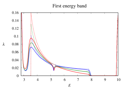
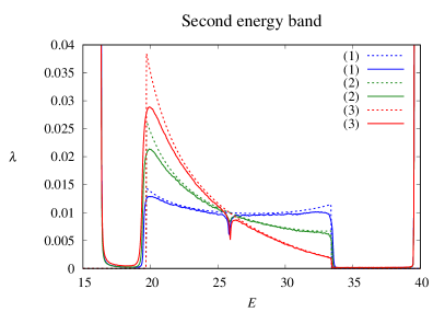
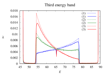
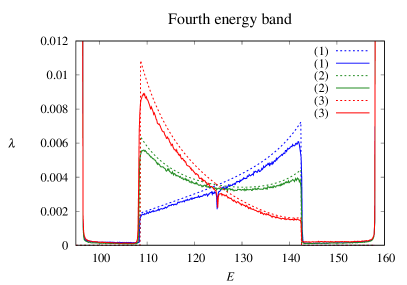
Figure 14: Lyapunov exponent $\lambda$ (in $\mbox{cm}^{-1}$) versus energy $E$ (in $\mbox{cm}^{-2}$) for the first 4 bands. The dotted lines correspond to the analytical expression (24); the solid lines represent the numerical values obtained using Eqs. (71) and (73). The data were obtained for the 2D Kronig-Penney model (57) with the following parameters: $U=4.0\,\mbox{cm}^{-1}$, $r_{1}=5\,\mbox{cm}$, and $a=1\,\mbox{cm}$. Disorder strength: $\sqrt{\langle u_{n}^{2}\rangle}=1.0\,\mbox{cm}^{-1}$ and $\sqrt{\langle\Delta_{n}^{2}\rangle}=0.02\,\mbox{cm}$. The mobility edges were set at $k_{1}=\pi/4$ and $k_{2}=\pi/2$. The data labelled with 1 (blue), 2 (green), and 3 (red) correspond to the cases of positive, absent, and negative cross-correlations. The rise of the Lyapunov exponent at the lower and upper parts of the windows corresponds to the band structure of the periodic system.

As can be seen from figure 14, the numerical data generally match the theoretical predictions for the Lyapunov exponent in a satisfactory way. A discrepancy occurs for $k=\pi/2$, where the Kronig-Penney model exhibits an anomaly which is the equivalent of the band-centre anomaly in the Anderson model, and where the expression (24) for the Lyapunov exponent fails as Thouless formula does at the band centre [54]. The band structure also corresponds to the theoretical expectations: this can be seen by considering that the points where the numerically computed Lyapunov exponent starts a rapid increase coincide with the band limits obtained by solving (20) for the 1D Kronig-Penney model (21). We show the band structure derived from (20) in figure 15.

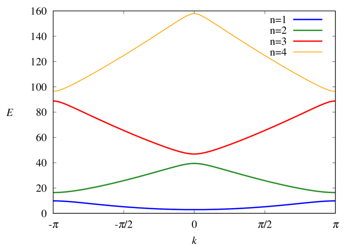
Figure 15: Energy $E$ (in $\mbox{cm}^{-2}$) versus the Bloch vector $k$ (dimensionless). The first four bands are represented, with the band index taking the values $n=1,2,3,4$. The data were obtained for $U=4.0\,\mbox{cm}^{-1}$ and $a=1\,\mbox{cm}$.

The data in figure 14 correspond to an s-wave, but the results do not change if we consider a particle in a different angular state. This is shown in figure 16, which represents the numerical values of the Lyapunov exponent in the second energy band for four values of the angular momentum ranging from $l=0$ to $l=50$. The data were obtained with the same values of the parameters used in figure 14.

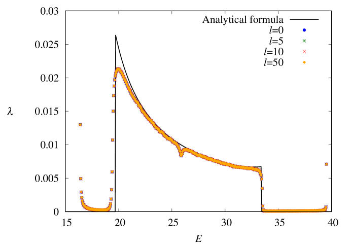
Figure 16: Lyapunov exponent $\lambda$ (in $\mbox{cm}^{-1}$) versus energy $E$ (in $\mbox{cm}^{-2}$) for several values of the angular momentum $l$. The considered values of the energy correspond to the second energy band. The data were obtained for the 2D Kronig-Penney model (57) with the following parameters: $U=4.0\,\mbox{cm}^{-1}$, $r_{1}=5\,\mbox{cm}$, and $a=1\,\mbox{cm}$. Disorder strength: $\sqrt{\langle u_{n}^{2}\rangle}=1.0\,\mbox{cm}^{-1}$ and $\sqrt{\langle\Delta_{n}^{2}\rangle}=0.02\,\mbox{cm}$. The mobility edges were set at $k_{1}=\pi/4$ and $k_{2}=\pi/2$. Structural and compositional disorder were not cross-correlated.

The complete collapse of the data corresponding to different values of $l$ confirms that the Lyapunov exponent does not depend on the angular momentum and shows that the centrifugal potential plays a negligible role in the localisation of the wavefunction.

In mathematical terms, this irrelevance is confirmed by considering the behaviour of the ratio $R_{n}$ in the limit of large $n$. In fact, for $n\gg 1$ one can use the asymptotic expansions for the Hankel functions

$$\begin{array}[]{ccl}H_{l}^{(1)}(z)&=&\displaystyle\sqrt{\frac{2}{\pi z}}e^{i\left(z-\frac{\pi}{2}l-\frac{\pi}{4}\right)}\left[1+i\frac{4l^{2}-1}{8}\frac{1}{z}+\ldots\right]\\ H_{l}^{(2)}(z)&=&\displaystyle\sqrt{\frac{2}{\pi z}}e^{-i\left(z-\frac{\pi}{2}l-\frac{\pi}{4}\right)}\left[1-i\frac{4l^{2}-1}{8}\frac{1}{z}+\ldots\right]\\ \end{array}$$

and write the map (73) in the simplified form

$$R_{n}\simeq-\frac{U_{n}}{U_{n-1}}e^{-i2\sqrt{E}\Delta_{n-1}}\frac{1}{R_{n-1}}+1-\frac{i}{2}\frac{U_{n}}{q}+\frac{U_{n}}{U_{n-1}}\left(1+\frac{i}{2}\frac{U_{n-1}}{\sqrt{E}}\right),$$ (74)

which does not show any dependence on the value of the angular momentum.

The asymptotic map (74) can also be used to confirm that the 1D model (21) and in its 2D counterpart (57) have the same band structure. To see this point, let us consider an eigenstate of the Schrödinger equation (51) in the $n$-th potential well having the form

$$\begin{array}[]{ccc}\displaystyle\psi_{\mathrm{out}}(r,\theta)=A_{n}H_{l}^{(1)}\left(\sqrt{E}r\right)e^{il\theta}&\mbox{ for }&r_{n}<r<r_{n+1}.\end{array}$$

The amplitude ratio $R_{n}$ can then be written

$$R_{n}=\frac{A_{n}}{A_{n-1}}=\frac{\psi_{\mathrm{out}}(r_{n},\theta)}{\psi_{\mathrm{out}}(r_{n-1},\theta)}\frac{H_{l}^{(1)}(\sqrt{E}r_{n-1})}{H_{l}^{(1)}(\sqrt{E}r_{n})}.$$

For $n\gg 1$ one can use the asymptotic expansion of the Hankel function and write

$$R_{n}\simeq\frac{\psi_{\mathrm{out}}(r_{n},\theta)}{\psi_{\mathrm{out}}(r_{n-1},\theta)}e^{-i\sqrt{E}\Delta_{n}}.$$ (75)

In the absence of disorder, and assuming that the centrifugal potential can be neglected for $r_{n}\to\infty$, one can expect that Bloch’s theorem applies and that increasing the radial coordinate of a lattice step $a$ should produce a change of phase in the wavefunction:

$$\frac{\psi^{\mathrm{out}}(r_{n},\theta)}{\psi_{\mathrm{out}}(r_{n-1},\theta)}\simeq e^{ik},$$

where $k$ is the Bloch wavevector. Substituting this expression in (75) and taking into account that without structural disorder $\Delta_{n}=a$, one obtains

$$R_{n}\simeq e^{i\left(k-\sqrt{E}a\right)}.$$ (76)

On the other hand, in the absence of disorder the asymptotic map (74) reduces to the form

$$R_{n}e^{i\sqrt{E}a}\simeq-\frac{1}{\displaystyle R_{n-1}e^{i\sqrt{E}a}}+2\cos\left(\sqrt{E}a\right)+\frac{U}{\sqrt{E}}\sin\left(\sqrt{E}a\right).$$ (77)

Substituting the expression (76) in (77), one recovers (20) with $q$ and $\alpha$ replaced by $\sqrt{E}$ and $a$. We have thus reached again the conclusion that the 1D model (21) and its 2D equivalent (56) have the same band structure.

4.4 The transmission coefficient

We now consider the transmission properties of an annulus with a finite number $N$ of circular barriers. As can be seen from (56) in this case the plane of motion is divided in three regions: a central disk with $r<r_{1}$ where the quantum particle is free, the annular region with $r_{1}\leq r\leq r_{N}$ where the particle is scattered by the $N$ barriers, and the plane beyond the last barrier with $r>r_{N}$, where the particle is free again. In the inner disk the solution can be written as a superposition of an incident and a reflected wave,

$$\begin{array}[]{ccc}R(r)=A_{0}H_{l}^{(1)}(\sqrt{E}r)+B_{0}H_{l}^{(2)}(\sqrt{E}r)&\mbox{ for }&r<r_{1}.\end{array}$$

while in the outer space only a transmitted wave is present

$$\begin{array}[]{ccc}R(r)=A_{N}H_{l}^{(1)}(\sqrt{E}r)&\mbox{ for }&r_{N}<r.\end{array}$$

Within the potential wells of the annulus, the solution is given by (68). The situation is graphically represented in figure 17.

Figure 17: Schematic representation of the impinging, reflected, and transmitted waves.

The amplitudes of the waves on both sides of the annulus can be linked with the total transfer matrix

$$\mathcal{M}_{N}=\mathbf{M}_{N}\mathbf{M}_{N-1}\cdots\mathbf{M}_{1}$$ (78)

with the individual transfer matrices defined by (70). One has

$$\left(\begin{array}[]{c}A_{N}\\ 0\\ \end{array}\right)=\mathcal{M}_{N}\left(\begin{array}[]{c}A_{0}\\ B_{0}\\ \end{array}\right).$$ (79)

We define the transmission coefficient as the ratio of the transmitted and incident probability currents

$$T_{N}=\frac{\displaystyle\int_{0}^{2\pi}\left.\left(\mathbf{j}_{\mathrm{out}}\cdot\hat{r}\right)\right|_{r=r_{N}}r_{N}\mathrm{d}\theta}{\displaystyle\int_{0}^{2\pi}\left.\left(\mathbf{j}_{\mathrm{in}}\cdot\hat{r}\right)\right|_{r=r_{1}}r_{1}\mathrm{d}\theta}$$ (80)

with

$$\mathbf{j}=-\frac{1}{2m}\left[\psi^{\ast}\hat{\mathbf{p}}\psi+\psi\left(\hat{\mathbf{p}}\psi\right)^{\ast}\right].$$

In (80) we integrate the probability current around the inner and outer rings of the annulus to compensate for the $1/\sqrt{r}$ decrease of the amplitude of the circular waves. In physical terms, this corresponds to using circular detectors to measure the intensity of the total impinging and outgoing waves. Taking into account that the incident and transmitted waves have the form

$$\psi_{\mathrm{in}}(r,\theta)=A_{0}H_{l}^{(1)}(\sqrt{E}r)e^{il\theta}$$

and

$$\psi_{\mathrm{out}}(r,\theta)=A_{N}H_{l}^{(1)}(\sqrt{E}r)e^{il\theta},$$

one obtains that the transmission coefficient (80) is equal to the squared ratio of the amplitudes of the outgoing and incoming waves

$$T_{N}=\left|\frac{A_{N}}{A_{0}}\right|^{2}.$$ (81)

Using (79) and the fact that $\det\mathcal{M}_{N}=1$, one can express the transmission coefficient (81) as

$$T_{N}=\frac{1}{\left|\left(\mathcal{M}_{N}\right)_{22}\right|^{2}}.$$ (82)

(82) can be used to compute numerically the transmission coefficient across the random annulus.

From the analytical point of view, knowledge of the inverse localisation length (24) is sufficient to determine the behaviour of the transmission coefficient in the localised regime: one has

$$\ln T_{N}\simeq-2\frac{r_{N}-r_{1}}{l_{\mathrm{loc}}}$$ (83)

for $(r_{N}-r_{1})\gg l_{\mathrm{loc}}$. In the metallic and intermediate regimes, i.e., for $(r_{N}~{}-~{}r_{1})~{}\lesssim~{}l_{\mathrm{loc}}$, the Lyapunov exponent does not determine the transmission coefficient completely. However, one can invoke the single-parameter scaling theory which, in the formulation of Pichard [71], postulates that the conductance $g$ of a 1D system of size $x$ can be expressed as a function $f(x/l_{\mathrm{loc}})$ of the ratio of the finite sample size to the localisation length in the infinite model. Pichard showed that the ansatz $g(x)=f(x/l_{\mathrm{loc}})$ is equivalent to the ordinary formulation $d\ln g/d\ln L=\beta(g)$ of the SPS hypothesis. His argument can be transposed without modification to the present case with the width $r_{N}-r_{1}$ of the annulus replacing the length $x$ of the random sample (although the specific form of the function $f$ need not be the same as in the 1D case studied in [71]). We can conclude that transmission across the random annulus depends on the ratio of the ring width $r_{N}-r_{1}$ to the localisation length $l_{\mathrm{loc}}$, i.e.,

$$T_{N}=F\left(\frac{r_{N}-r_{1}}{l_{\mathrm{loc}}}\right).$$ (84)

The single-parameter scaling theory leaves unspecified the form of the function $F(x)$; however (84) still allows one to make significant predictions: in particular, one can conclude that the transmission coefficient approaches a unitary value whenever $\lambda\to 0$.

In figures 18, 19, and 20 we compare the data obtained by numerical evaluation of the transmission coefficient (82) with the analytical formula (83). We determined the transmission coefficient for the Kronig-Penney model (56) with a finite number $N$ of barriers; we considered the values $N=30$, $N=100$, and $N=300$. We selected the same values of the parameters already used in Sec. 4.3, i.e., $U=4.0\,\mbox{cm}^{-1}$, $r_{1}=5\,\mbox{cm}$, and $a=1\,\mbox{cm}$. We set the disorder strengths at $\sqrt{\langle u_{n}^{2}\rangle}=1.0\,\mbox{cm}^{-1}$ and $\sqrt{\langle\Delta_{n}^{2}\rangle}=0.02\,\mbox{cm}$ and we put mobility edges at $k_{1}=\pi/4$ and $k_{2}=\pi/2$. The numerical data were obtained for an s-wave, but the results do not change if different values of the angular momentum $l$ are selected. In order to obtain a better understanding of the behaviour of the transmission coefficient as a function of the energy of the incoming wave, we averaged $\ln T_{N}$ over an ensemble of $N_{r}=1000$ disorder realisations, thus eliminating the fluctuations associated to each individual realisation of the disorder.

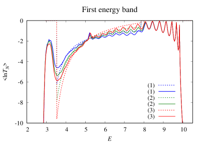
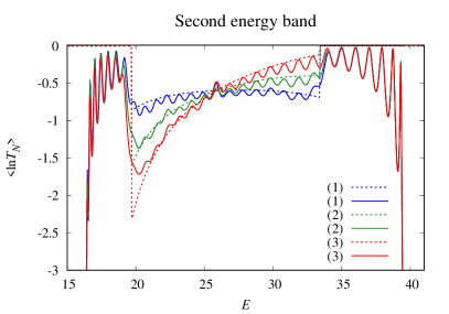
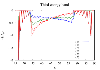
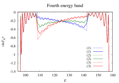
Figure 18: Average of the logarithm of the transmission coefficient $\langle\ln T_{N}\rangle$ versus energy $E$ (in $\mbox{cm}^{-2}$) for $N=30$ barriers. Each panel represents one of the first four energy bands. The dotted lines correspond to the analytical expression (83); the solid lines correspond to the numerical evaluation of (82). The average was computed over an ensemble of $N_{r}=1000$ disorder realisations. The data were obtained for the 2D Kronig-Penney model (56) with the following parameters: $U=4.0\,\mbox{cm}^{-1}$, $r_{1}=5\,\mbox{cm}$, and $a=1\,\mbox{cm}$. Disorder strength: $\sqrt{\langle u_{n}^{2}\rangle}=1.0\,\mbox{cm}^{-1}$ and $\sqrt{\langle\Delta_{n}^{2}\rangle}=0.02\,\mbox{cm}$. The mobility edges were set at $k_{1}=\pi/4$ and $k_{2}=\pi/2$. The data labelled with 1 (blue), 2 (green), and 3 (red) correspond to the cases of positive, absent, and negative cross-correlations.

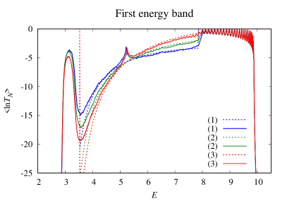
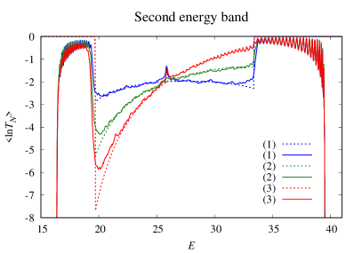
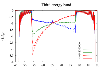
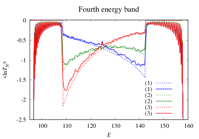
Figure 19: As figure 18 but for $N=100$ barriers.

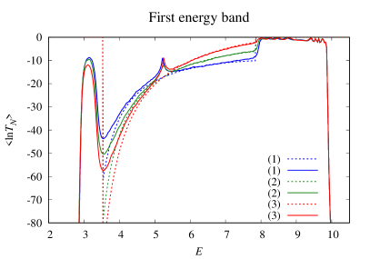
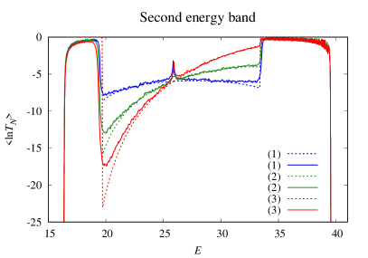
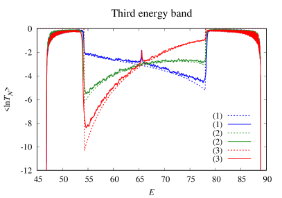
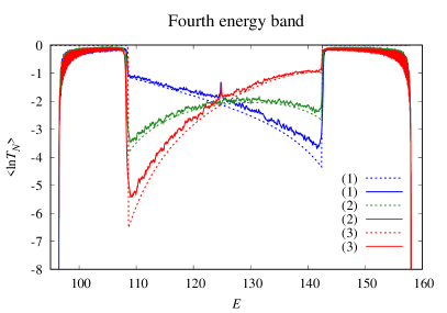
Figure 20: As figure 18 but for $N=300$ barriers.

The numerical data show that formula (83) describes the behaviour of the transmission coefficient well when the number of barriers is large ($N\sim 300$); the formula works reasonably well also in the case in which the number of barriers is reduced ($N\sim 30$) or intermediate ($N\sim 100$), although in these cases (83) fails to reproduce the oscillations of $\ln T_{N}$ with $E$.

Figures 18, 19, and 20 clearly show that the use of correlated disorder to effectively suppress transmission in predefined energy windows is not restricted to 1D models but works well also in 2D systems. As expected the windows where transmission is inhibited correspond to the energy intervals where correlated disorder enhances the localisation and increases the Lyapunov exponent. As a consequence, transmission is permitted (in fact, it is enhanced) only in the windows where the Lyapunov exponent tends to zero. We can conclude that the use of correlated disorder makes possible to generate small transmission bands for which the annulus becomes almost completely transparent. By moving the mobility edges, one can thus select the energy of the transmitted waves and use the annulus as a band filter.

5 Conclusions

In this work we have studied the localisation and transport properties of 2D models with Hamiltonians that are separable in polar coordinates and have random potentials that depend on a single variable, $r$ or $\theta$. Broadly speaking, our analysis confirms what one would intuitively expect for such models: mathematically, the separability condition allows one to study these 2D systems in terms of models of lower dimensionality; physically, localisation occurs on the coordinate associated with the random part of the potential. These conclusions, however, come with several caveats and putting them on a firm footing required a precise assessment of the analogies and differences which exist between the 2D models under study and their 1D counterparts.

In the case of models with angular disorder, we found that the geometry of the 2D problem sets unavoidable constraints on the 1D associated model: first and foremost, the 1D model has a finite size and its wavefunctions must satisfy periodic boundary conditions. In ordinary 1D models the finite size of the random sample can be neglected if disorder is sufficiently strong to produce localisation on a length scale smaller than the system size. This possibility is partially precluded in the present case, because the geometry of the 2D model imposes severe constraints on the strength of structural disorder. A good degree of localisation can be achieved even for weak disorder, however, if long-range correlations of the random potential are appropriately used to this effect. Mathematically, the finite size of the system complicates the analysis of its eigenfunctions: it is not possible to study the tails of the eigenstates by considering the asymptotic behaviour of products of transfer matrices because one deals with a finite and limited number of transfer matrices. To determine the localisation properties of the 2D model we had to resort to the direct evaluation of the eigenstates of the associated tight-binding model which is the 1D discrete counterpart of the original 2D system. In so doing, however, we had to take into account that the correspondence between discrete and continuous models can be tricky when resonance phenomena come into play. In fact, we found that a striking feature of the 2D model with random angular potential lies in the fact that its eigenstates are shaped not only by localisation, but also by Fabry-Pérot resonances which occur when the ratio of the angular momentum to the angular width of a potential well is an integer multiple of $\pi$.

In the case of 2D models with a central random potential, we have shown that the localisation of the radial part of the wavefunction occurs exactly as in the 1D case provided that the random potential falls off away from the force centre more slowly than the centrifugal potential. This circumstance can be exploited to reproduce in 2D models the localisation-delocalisation transitions that are generated in 1D systems by specific long-range correlations of the disorder. In this way one can design 2D filters which allow the transmission of waves within predefined frequency windows, thus overcoming the limitations of the 1D geometry of previous devices of this kind.

As a final remark, we would like to point out that in this paper we restricted our attention to 2D models. The present approach, however, can be applied also to 3D models with similar features; we plan to extend our results to this class of system in a future paper.

Appendix A Application to microwave cavities

In this appendix we discuss how the model (1) can be applied to different physical problems beyond that of a quantum particle in an annulus. Specifically, we show how a slight modification of (1) can be reinterpreted as the Helmholtz equation describing the electric field of a transverse magnetic (TM) mode in a microwave cavity shaped as a ring cake tin.

In fact, one can consider a microwave cavity vertically bounded by two coaxial cylinders (of radii $r_{1}$ and $r_{2}$) and closed at the bottom and at the top by two horizontal plates separated by a distance $d_{0}$. It is natural to introduce cylindrical coordinates and to set the $z$-axis along the cylinder axis. If one assumes that the top and bottom plates of the cavity are flat, the electric field of the $m$-th TM mode can be written in the form

$$\mathbf{E}_{TM}(r,\theta,z)=E_{z}(r,\theta)\sin\left(\frac{m\pi}{d_{0}}z\right)\mathbf{\hat{z}}$$

with the amplitude $E_{z}(r,\theta)$ satisfying the wave equation

$$\left[-\nabla^{2}+\left(\frac{m\pi}{d_{0}}\right)^{2}\right]E_{z}(r,\theta)=\frac{\omega^{2}}{c^{2}}E_{z}(r,\theta)$$ (85)

where $\nabla^{2}$ is the 2D Laplacian (2).

If the top and bottom plates are not perfectly flat, so that the distance $d(r,\theta)$ between them is not constant, (85) ceases to be exact. It remains approximately satisfied, however, if the distance $d(r,\theta)$ changes slowly with the position. In this case it is convenient to rewrite (85) in the form

$$\left\{-\nabla^{2}+\left[\left(\frac{m\pi}{d(r,\theta)}\right)^{2}-\left(\frac{m\pi}{d_{\mathrm{m}ax}}\right)^{2}\right]\right\}E_{z}(r,\theta)=\left[\frac{\omega^{2}}{c^{2}}-\left(\frac{m\pi}{d_{\mathrm{m}ax}}\right)^{2}\right]E_{z}(r,\theta),$$ (86)

where $d_{\mathrm{m}ax}$ represents the maximum distance between the top and bottom plates. The term $(m\pi/d(r,\theta))^{2}$ in the left-hand side of (86) plays the role of a potential; from this point of view, subtracting the constant term $(m\pi/d_{\mathrm{max}})^{2}$ is equivalent to setting the potential equal to zero on the bottom plate of the cavity.

Comparing Eqs. (1) and (86), one can see that they have identical forms and that the same mathematical solutions describe the wavefunction $\psi(r,\theta)$ and the longitudinal electric field $E_{z}(r,\theta)$. We observe that the energy of the quantum particle in model (1) and the frequency of the electric field in the cavity (86) are connected as follows

$$E=\frac{\omega^{2}}{c^{2}}-\left(\frac{m\pi}{d_{\mathrm{max}}}\right)^{2};$$

the potential $U(r,\theta)$ and the distance $d(r,\theta)$, on the other hand, are related by the identity

$$U(r,\theta)=m^{2}\pi^{2}\left[\frac{1}{d^{2}(r,\theta)}-\frac{1}{d_{\mathrm{m}ax}^{2}}\right].$$ (87)

(87) shows how the potential $U(r,\theta)$ in the quantum mechanical model (1) can be reproduced with an appropriate topographical shape of the bottom plate in a microwave cavity. Obviously, there is no way to reproduce physically the $\delta$-barriers in the potential (5); the latter, however, should be seen as a schematic representation of a real potential of the form

$$U_{\varepsilon}(r,\theta)=\frac{1}{r^{2}}\sum_{n=1}^{N}U_{n}\eta_{\varepsilon}(\theta-\theta_{n})$$

with

$$\eta_{\varepsilon}(\theta)=\left\{\begin{array}[]{ccc}\displaystyle\frac{1}{2\varepsilon}&\mbox{ if }&\theta\in[-\varepsilon,\varepsilon]\\ 0&\mbox{ if }&\theta\notin[-\varepsilon,\varepsilon]\\ \end{array}\right.$$

where $\varepsilon$ is a small positive parameter. A potential of this kind can be reproduced by inserting appropriately shaped wedges in a ring microwave cavity.

We observe that the theoretical predictions obtained with the use of the 1D Kronig-Penney model with $\delta$-barriers have worked remarkably well when applied to quasi-1D waveguides with physical barriers of various shapes and kinds (screws in [72], bars in [56]). In light of the past experience, we expect that the use of models with $\delta$-barriers should produce reasonable results even for 2D cavities with rectangular wedges, provided that the width of the barriers is sufficiently smaller than $1/k_{\theta}$, where $k_{\theta}$ is the wavenumber in the angular direction. We would like to emphasise as well that in the weak-disorder limit the localisation length essentially depends on the binary correlator of the random potential, rather than on the potential itself. Although specific details, like the value of the Lyapunov exponent, the exact frequencies for which mobility edges appear and the spatial location of the localisation centres do depend on the form of the potential, the general features of the spectral shaping of the localisation length should still be observable even when the $\delta$-barrier potential does not represent too closely the actual potential in the experimental setup, assuming that the disorder correlations are the same.

Appendix B Generation of self- and cross-correlated random sequences

In this appendix we summarise how one can generate two random sequences $\{u_{n}\}$ and $\{\Delta_{n}\}$ with pre-defined self- and cross-correlations. As a first step, one generates two uncorrelated sequences $\{X_{n}^{(1)}\}$ and $\{X_{n}^{(2)}\}$ of independent variables. The two white noises are then cross-correlated via the transformation

$$\begin{array}[]{ccl}Y_{n}^{(1)}&=&X_{n}^{(1)}\cos\eta+X_{n}^{(2)}\sin\eta\\ Y_{n}^{(2)}&=&X_{n}^{(1)}\sin\eta+X_{n}^{(2)}\cos\eta,\\ \end{array}$$

where $\eta$ is the parameter which determines the degree of cross-correlation of the $Y_{n}^{(1)}$ and $Y_{n}^{(2)}$ sequences. Finally one filters the cross-correlated white noises $Y_{n}^{(1)}$ and $Y_{n}^{(2)}$ so that they acquire the desired self-correlation properties. The operation is carried out with the convolution products

$$\begin{array}[]{ccl}u_{n}&=&\displaystyle\sum_{l=-\infty}^{\infty}c^{(1)}_{l}Y_{n-l}^{(1)}\\ \Delta_{n}&=&\displaystyle\sum_{l=-\infty}^{\infty}c^{(2)}_{l}Y_{n-l}^{(2)}\\ \end{array},$$ (88)

in which the coefficients $c^{(1)}_{n}$ and $c^{(2)}_{n}$ are derived by the pre-defined power spectra $W_{1}$ and $W_{2}$ with the help of the following identities

$$\begin{array}[]{ccl}c^{(1)}_{n}&=&\displaystyle\frac{2}{\pi}\int_{0}^{\pi/2}\sqrt{\langle u_{l}^{2}\rangle W_{1}(x)}\cos\left(2nx\right)\mathrm{d}x\\ c^{(2)}_{n}&=&\displaystyle\frac{2}{\pi}\int_{0}^{\pi/2}\sqrt{\langle\Delta_{l}^{2}\rangle W_{2}(x)}\cos\left(2nx\right)\mathrm{d}x.\\ \end{array}$$

Appendix C Explicit form of the matrix terms in expansions (65) and (66)

In this appendix we provide the explicit form of the matrices that appear in the expansions (65) and (66). In the rhs of (65), the zero-th order term $\mathbf{T}_{n}^{(0)}$ has matrix elements

$$\begin{array}[]{ccl}\left({\mathbf{T}}_{n}^{(0)}\right)_{11}&=&\displaystyle\cos\left[\sqrt{E}\left(a+\Delta_{n}\right)\right]+\frac{U_{n}}{\sqrt{E}}\sin\left[\sqrt{E}\left(a+\Delta_{n}\right)\right]\\ \left({\mathbf{T}}_{n}^{(0)}\right)_{12}&=&\displaystyle\frac{1}{\sqrt{E}}\sin\left[\sqrt{E}\left(a+\Delta_{n}\right)\right]\\ \left({\mathbf{T}}_{n}^{(0)}\right)_{21}&=&\displaystyle-\sqrt{E}\sin\left[\sqrt{E}\left(a+\Delta_{n}\right)\right]+U_{n}\cos\left[\sqrt{E}\left(a+\Delta_{n}\right)\right]\\ \left({\mathbf{T}}_{n}^{(0)}\right)_{11}&=&\displaystyle\cos\left[\sqrt{E}\left(a+\Delta_{n}\right)\right]\\ \end{array}$$

while the matrix elements of the second-order term $\mathbf{T}_{n}^{(2)}$ are

$$\begin{array}[]{ccl}\left({\mathbf{T}}_{n}^{(2)}\right)_{11}&=&\displaystyle-\frac{l^{2}-1/4}{2\sqrt{E}}\left\{\left[\frac{1}{E}U_{n}-a-\Delta_{n}\right]\sin[\sqrt{E}(a+\Delta_{n})]\right.\\ &+&\displaystyle\left.\frac{1}{\sqrt{E}}U_{n}(a+\Delta_{n})\cos[\sqrt{E}(a+\Delta_{n})]\right\}\\ \left({\mathbf{T}}_{n}^{(2)}\right)_{12}&=&\displaystyle\frac{l^{2}-1/4}{2\sqrt{E}}\left\{-\frac{1}{E}\sin\left[\sqrt{E}\left(a+\Delta_{n}\right)\right]\right.\\ &+&\displaystyle\left.\frac{1}{\sqrt{E}}(a+\Delta_{n})\cos\left[\sqrt{E}\left(a+\Delta_{n}\right)\right]\right\}\\ \left({\mathbf{T}}_{n}^{(2)}\right)_{21}&=&\displaystyle-\frac{l^{2}-1/4}{2\sqrt{E}}\left\{\left[1+U_{n}(a+\Delta_{n})\right]\sin\left[\sqrt{E}\left(a+\Delta_{n}\right)\right]\right.\\ &-&\displaystyle\left.\sqrt{E}(a+\Delta_{n})\cos\left[\sqrt{E}\left(a+\Delta_{n}\right)\right]\right\}\\ \left({\mathbf{T}}_{n}^{(2)}\right)_{21}&=&\displaystyle-\frac{l^{2}-1/4}{2\sqrt{E}}(a+\Delta_{n})\sin\left[\sqrt{E}\left(a+\Delta_{n}\right)\right].\\ \end{array}$$

In expansion (66), the unperturbed term is equal to

$${\mathbf{T}}_{n}^{(0,0)}=\left(\begin{array}[]{cc}\displaystyle\cos(\sqrt{E}a)+\frac{U}{\sqrt{E}}\sin(\sqrt{E}a)&\displaystyle\frac{1}{\sqrt{E}}\sin(\sqrt{E}a)\\ -\sqrt{E}\sin(\sqrt{E}a)+U\cos(\sqrt{E}a)&\cos(\sqrt{E}a)\\ \end{array}\right).$$

The dominant corrections due to disorder are the random matrices $\mathbf{T}_{n}^{(1,0)}$ and $\mathbf{T}_{n}^{(2,0)}$, with elements

$$\begin{array}[]{ccl}\left({\mathbf{T}}_{n}^{(1,0)}\right)_{11}&=&\displaystyle\frac{1}{\sigma}\left[\Delta_{n}U\cos(\sqrt{E}a)+\left(\frac{u_{n}}{\sqrt{E}}-\sqrt{E}\Delta_{n}\right)\sin(\sqrt{E}a)\right]\\ \left({\mathbf{T}}_{n}^{(1,0)}\right)_{12}&=&\displaystyle\frac{\Delta_{n}}{\sigma}\cos(\sqrt{E}a)\\ \left({\mathbf{T}}_{n}^{(1,0)}\right)_{21}&=&\displaystyle\frac{1}{\sigma}\left[\left(u_{n}-E\Delta_{n}\right)\cos(\sqrt{E}a)-\sqrt{E}U\sin(\sqrt{E}a)\right]\\ \left({\mathbf{T}}_{n}^{(1,0)}\right)_{22}&=&\displaystyle-\sqrt{E}\frac{\Delta_{n}}{\sigma}\sin(\sqrt{E}a)\\ \end{array}$$

and

$$\begin{array}[]{ccl}\left({\mathbf{T}}_{n}^{(2,0)}\right)_{11}&=&\displaystyle\frac{1}{\sigma^{2}}\left[\left(u_{n}\Delta_{n}-\frac{1}{2}E\Delta_{n}^{2}\right)\cos(\sqrt{E}a)-\frac{1}{2}U\sqrt{E}\Delta_{n}^{2}\sin(\sqrt{E}a)\right]\\ \left({\mathbf{T}}_{n}^{(2,0)}\right)_{12}&=&\displaystyle-\frac{1}{2}\sqrt{E}\frac{\Delta_{n}^{2}}{\sigma^{2}}\sin(\sqrt{E}a)\\ \left({\mathbf{T}}_{n}^{(2,0)}\right)_{21}&=&\displaystyle\frac{1}{\sigma^{2}}\left[-\frac{1}{2}EU\Delta_{n}^{2}\cos(\sqrt{E}a)+\sqrt{E}\left(E\Delta_{n}^{2}-u_{n}\Delta_{n}\right)\sin(\sqrt{E}a)\right]\\ \left({\mathbf{T}}_{n}^{(2,0)}\right)_{22}&=&\displaystyle-\frac{1}{2}E\frac{\Delta_{n}^{2}}{\sigma^{2}}\cos(\sqrt{E}a)\\ \end{array}$$

The leading correction due to the centrifugal potential, on the other hand, is proportional to the matrix $\mathbf{T}_{n}^{(0,2)}$, whose elements are

$$\begin{array}[]{ccl}\left({\mathbf{T}}_{n}^{(0,2)}\right)_{11}&=&\displaystyle\frac{l^{2}-1/4}{2\sqrt{E}}\left[\frac{U}{E}\sin(\sqrt{E}a)-\frac{U}{\sqrt{E}}a\cos(\sqrt{E}a)\right]\\ \left({\mathbf{T}}_{n}^{(0,2)}\right)_{12}&=&\displaystyle\frac{l^{2}-1/4}{2\sqrt{E}}\left[-\frac{1}{E}\sin(\sqrt{E}a)+\frac{1}{\sqrt{E}}a\cos(\sqrt{E}a)\right]\\ \left({\mathbf{T}}_{n}^{(0,2)}\right)_{21}&=&\displaystyle\frac{l^{2}-1/4}{2\sqrt{E}}\left[(1+Ua)\sin(\sqrt{E}a)+\sqrt{E}a\cos(\sqrt{E}a)\right]\\ \left({\mathbf{T}}_{n}^{(0,2)}\right)_{22}&=&\displaystyle-\frac{l^{2}-1/4}{2\sqrt{E}}a\sin(\sqrt{E}a).\\ \end{array}$$

References

- Anderson [1958] P. W. Anderson. Absence of diffusion in certain random lattices. Phys. Rev., 109:1492, 1958. doi: 10.1103/PhysRev.109.1492.
- Thouless [1974] D. J. Thouless. Electrons in disordered systems and the theory of localization. Phys. Rep., 13:93, 1974. doi: 10.1016/0370-1573(74)90029-5.
- Lee and Ramakrishnan [1985] P. A. Lee and T. V. Ramakrishnan. Disordered electronic systems. Rev. Mod. Phys., 57:287, 1985. doi: 10.1103/RevModPhys.57.287.
- Evers and Mirlin [2008] F. Evers and A. D. Mirlin. Anderson transitions. Rev. Mod. Phys., 80:1355, 2008. doi: 10.1103/RevModPhys.80.1355.
- Kramer and MacKinnon [1993] B. Kramer and A. MacKinnon. Localization: theory and experiment. Rep. Prog. Phys., 56:1469, 1993. doi: 10.1088/0034-4885/56/12/001.
- Imry [2002] Y. Imry. Introduction to Mesoscopic Physics. University Press, Oxford, 2002.
- Tatarskii [1961] V.I. Tatarskii. Wave Propagation in a Turbulent Medium. Mc-Graw-Hill, New York, 1961.
- Chernov [1967] L.A. Chernov. Waves Propagation in a Random Medium. Dover, New York, 1967.
- Kravtsov [1992] Yu. A. Kravtsov. Propagation of electromagnetic waves through a turbulent atmosphere. Rep. Prog. Phys., 55:39, 1992. doi: 10.1088/0034-4885/55/1/002.
- Sheng [2006] P. Sheng. Introduction to Wave Scattering, Localization and Mesoscopic Phenomena, 2nd ed. Springer Verlag, Berlin, 2006.
- Chabanov et al. [2000] A. A. Chabanov, M. Stoytchev, and A. Z. Genack. Statistical signatures of photon localization. Nature, 404:850, 2000. doi: 10.1038/35009055.
- Sanchez-Palencia et al. [2007] L. Sanchez-Palencia, D. Clément, P. Lugan, P. Bouyer., G. V. Shlyapnikov, and A. Aspect. Anderson Localization of Expanding Bose-Einstein Condensates in Random Potentials. Phys. Rev. Lett., 98:210401, 2007. doi: 10.1103/PhysRevLett.98.210401.
- Billy et al. [2008] J. Billy, V. Josse, Z. Zuo, A. Bernard, B. Hambrecht, P. Lugan, D. Clément, L. Sanchez-Palencia, P. Bouyer, and A. Aspect. Direct observation of Anderson localization of matter waves in a controlled disorder. Nature, 453:891, 2008. doi: 10.1038/nature07000.
- Gurevich et al. [2009] E. Gurevich and O. Kenneth. Lyapunov exponent for the laser speckle potential: A weak disorder expansion Phys. Rev. A, 79:063617, 2009. doi: 10.1103/PhysRevA.79.063617.
- Aspect and Inguscio [2009] A. Aspect and M. Inguscio. Anderson localization of ultracold atoms. Physics Today, 62:30, 2009. doi: 10.1063/1.3206092.
- Lugan et al. [2009] P. Lugan, A. Aspect, L. Sanchez-Palencia, D. Delande, B. Grémaud, C. A. Müller, and C. Minatura. One-dimensional Anderson localization in certain correlated random potentials Phys. Rev. A, 80:023605, 2009. doi: 10.1103/PhysRevA.80.023605.
- Sanchez-Palencia and Lewenstein [2010] L. Sanchez-Palencia and M. Lewenstein. Disordered quantum gases under control. Nat. Phys., 6:87, 2010. doi: 10.1038/nphys1507.
- Modugno [2010] G. Modugno. Anderson localization in Bose-Einstein condensates. Rep. Prog. Phys., 73:102401, 2010. doi: 10.1088/0034-4885/73/10/102401.
- Piraud et al. [2011] M. Piraud, P. Lugan, P. Bouyer, A. Aspect, and L. Sanchez-Palencia. Localization of a matter wave packet in a disordered potential. Phys. Rev. A, 83:031603(R), 2011. doi: 10.1103/PhysRevA.83.031603.
- Shapiro [2012] B. Shapiro. Cold atoms in the presence of disorder. J. Phys. A, 45:143001, 2012. doi: 10.1088/1751-8113/45/14/143001.
- Piraud et al. [2013] M. Piraud and L. Sanchez-Palencia. Tailoring Anderson localization by disorder correlations in 1D speckle potentials Eur. Phys. J. Special Topics, 217:91, 2013. doi: 10.1140/epjst/e2013-01758-6.
- Wiersma et al. [1997] D. S. Wiersma, P. Bartolini, A. Lagendijk, and R. Righini. Localization of light in a disordered medium. Nature, 390:671, 1997. doi: 10.1038/37757.
- Störzer et al. [2006] M. Störzer, P. Gross, C. M. Aegerter, and G. Maret. Observation of the critical regime near Anderson localization of light. Phys. Rev. Lett., 96:063904, 2006. doi: 10.1103/PhysRevLett.96.063904.
- Schwartz et al. [2007] T. Schwartz, G. Bartal, S. Fishman, and M. Segev. Transport and Anderson localization in disordered two-dimensional photonic lattices. Nature, 446:52, 2007. doi: 10.1038/nature05623.
- Skipetrov and Sokolov [2014] S.E. Skipetrov and I.M. Sokolov. Absence of anderson localization of light in a random ensemble of point scatterers. Phys. Rev. Lett., 112:023905, 2014. doi: 10.1103/PhysRevLett.112.023905.
- Sperling et al. [2016] T. Sperling, L. Schertel, M. Ackermann, G.J. Aubry, C.M. Aegerter, and G. Maret. Can 3d light localization be reached in ‘white paint’? New J. of Physics, 18:013039, 2016. doi: 10.1088/1367-2630/18/1/013039.
- Mott and Twose [1961] N. F. Mott and W. D. Twose. The theory of impurity conduction. Adv. Phys., 10:107, 1961. doi: 10.1080/00018736100101271.
- Izrailev et al. [2012] F. M. Izrailev, A. A. Krokhin, and N. M. Makarov. Anomalous localization in low-dimensional systems with correlated disorder. Phys. Rep., 512:125, 2012. doi: 10.1016/j.physrep.2011.11.002.
- Abrahams et al. [1979] E. Abrahams, P. W. Anderson, D. C. Licciardello, and T. V. Ramakrishnan. Scaling theory of localization: Absence of quantum diffusion in two dimensions. Phys. Rev. Lett., 42:673, 1979. doi: 10.1103/PhysRevLett.42.673.
- Anderson et al. [1980] P. W. Anderson, D. J. Thouless, E. Abrahams, and D. S. Fisher. New method for a scaling theory of localization. Phys. Rev. B, 22:3519, 1980. doi: 10.1103/PhysRevB.22.3519.
- Thouless [1982] D. J. Thouless. Lower dimensionality and localization. Physica B, 109-110:1523, 1982. doi: 10.1016/0378-4363(82)90174-7.
- Abrahams et al. [2001] E. Abrahams, S. V. Kravchenko, and M. P. Sarachik. Metallic behavior and related phenomena in two dimensions. Rev. Mod. Phys., 73:251, 2001. doi: 10.1103/RevModPhys.73.251.
- Gor’kov et al. [1979] L. P. Gor’kov, A. I. Larkin, and D. E. Khmel’nitskiĭ. Particle conductivity in a two-dimensional random potential. JETP Lett., 30:228, 1979. URL www.jetpletters.ac.ru/ps/1364/article_20629.shtml.
- MacKinnon and Kramer [1981] A. MacKinnon and B. Kramer. One-parameter scaling of localization length and conductance in disordered systems. Phys. Rev. Lett., 47:1546, 1981. doi: 10.1103/PhysRevLett.47.1546.
- Lee and Fisher [1981] P. A. Lee and D. S. Fisher. Anderson localization in two dimensions. Phys. Rev. Lett., 47:882, 1981. doi: 10.1103/PhysRevLett.47.882.
- Schreiber and Ottomeier [1992] M. Schreiber and M. Ottomeier. Localization of electronic states in 2D disordered systems. J. Phys.: Condens. Matter, 4:1959, 1992. doi: 10.1088/0953-8984/4/8/011.
- Tit and Schreiber [1995] N. Tit and M. Schreiber. The multifractal character of the electronic states in disordered two-dimensional systems. J. Phys.: Condens. Matter, 7:5549, 1995. doi: 10.1088/0953-8984/7/28/012.
- Eilmes et al. [1998] A. Eilmes, R. A. Römer, and M. Schreiber. The two-dimensional Anderson model of localization with random hopping. Eur. Phys. J. B, 1:29, 1998. doi: 10.1007/s100510050149.
- Unge and Stafström [2003] M. Unge and S. Stafström. Anderson localization in two-dimensional disordered systems. Synthetic Metals, 139:239, 2003. doi: 10.1016/S0379-6779(03)00125-5.
- Dorokhov [1982] O. N. Dorokhov. Transmission coefficient and the localization length of an electron in N bound disordered chains. JETP Lett., 36:318, 1982. URL www.jetpletters.ac.ru/ps/1335/article_27160.shtml.
- Mello et al. [1988] P. A. Mello, P. Pereyra, and N. Kumar. Macroscopic approach to multichannel disordered conductors. Ann. Phys. (N.Y.), 181:290, 1988. doi: 10.1016/0003-4916(88)90169-8.
- Markoš [2010] P. Markoš. Two-dimensional electron systems beyond the diffusive regime. Phys. Rev. B, 82:094203, 2010. doi: 10.1103/PhysRevB.82.094203.
- Moura et al. [2004] F. A. B. F. de Moura, M. D. Coutinho-Filho, M. L. Lyra, and E. P. Raposo. Delocalization and ballistic dynamics in the two-dimensional Anderson model with long-range correlated disorder. Europhys. Lett., 66:585, 2004. doi: 10.1209/epl/i2003-10238-4.
- dos Santos et al. [2007] I. F. dos Santos, F. A. B. F. de Moura, M. L. Lyra, and M. D. Coutinho-Filho. Critical behavior of the two-dimensional Anderson model with long-range correlated disorder. J. Phys.: Condens. Matter, 19:476213, 2007. doi: 10.1088/0953-8984/19/47/476213.
- Moura and Domínguez-Adame [2008] F. A. B. F. de Moura and F. Domínguez-Adame. Extended modes and energy dynamics in two-dimensional lattices with correlated disorder. Eur. Phys. J. B, 66:165, 2008. doi: 10.1140/epjb/e2008-00393-4.
- Moura [2010] F. A. B. F. de Moura. Absence of localization on the 2d model with long-range correlated off-diagonal disorder. Eur. Phys. J. B, 78:335, 2010. doi: 10.1140/epjb/e2010-10579-8.
- Plodzien et al. [2011] M. Plodzień and K Sacha. Matter-wave analog of an optical random laser. Phys. Rev. A, 84:023624, 2011. doi: 10.1103/PhysRevA.84.023624
- Piraud et al. [2012] M. Piraud, A. Aspect, and L. Sanchez-Palencia. Anderson localization of matter waves in tailored disordered potentials. Phys. Rev. A, 85:063611, 2012. doi: 10.1103/PhysRevA.85.063611
- Capuzzi et al. [2015] P. Capuzzi, M. Gattobigio, and P. Vignolo. Enhancing quantum coherence with short-range correlated disorder. Phys. Rev. A, 92:053622, 2015. doi: 10.1103/PhysRevA.92.053622.
- Barkhofen et al. [2013] S. Barkhofen, J. J. Metzger, R. Fleischmann, U. Kuhl, and H.-J. Stöckmann. Experimental observation of a fundamental length scale of waves in random media. Phys. Rev. Lett., 111:183902, 2013. doi: 10.1103/PhysRevLett.111.183902.
- Barboza et al. [2013] R. Barboza, U. Bortolozzo, G. Assanto, E. Vidal-Henriquez, M. G. Clerc, and S. Residori. Harnessing optical vortex lattices in nematic liquid crystals. Phys. Rev. Lett., 111:093902, 2013 doi: 10.1103/PhysRevLett.111.093902.
- Lifshits, Gredeskul, Pastur [1988] I. M. Lifshits, S. A. Gredeskul, and L. A. Pastur. Introduction to the Theory of Disordered Systems. Wiley Interscience, New York, 1988.
- Hernández-Herrejón et al. [2008] J. C. Hernández-Herrejón, F. M. Izrailev, and L. Tessieri. Anomalous properties of the Kronig-Penney model with compositional and structural disorder. Physica E, 40:3137, 2008. doi: 10.1016/j.physe.2008.05.001.
- Hernández-Herrejón et al. [2010a] J. C. Hernández-Herrejón, F. M. Izrailev, and L. Tessieri. Anomalous localization in the aperiodic Kronig-Penney model. J. Phys. A, 43:425004, 2010a. doi: 10.1088/1751-8113/43/42/425004.
- Hernández-Herrejón et al. [2010b] J. C. Hernández-Herrejón, F. M. Izrailev, and L. Tessieri. Electronic states and transport properties in the Kronig-Penney model with correlated compositional and structural disorder. Physica E, 42:2203, 2010b. doi: 10.1016/j.physe.2010.04.020.
- Dietz et al. [2012] O. Dietz, U. Kuhl, J. C. Hernández-Herrejón, and L. Tessieri. Transmission in waveguides with compositional and structural disorder: experimental effects of disorder cross-correlations. New J. of Physics, 14(1):013048, 2012. doi: 10.1088/1367-2630/14/1/013048.
- Kuhl et al. [2008] U. Kuhl, F. M. Izrailev, and A. A. Krokhin. Enhancement of localization in one-dimensional random potentials with long-range correlations. Phys. Rev. Lett., 100:126402, 2008. doi: 10.1103/PhysRevLett.100.126402.
- Tessieri et al. [2015] L. Tessieri, I. F. Herrera-González, and F. M. Izrailev. The band-centre anomaly in the 1D Anderson model with correlated disorder. J. Phys. A, 48:355001, 2015. doi: 10.1088/1751-8113/48/35/355001.
- Wegner [1980] F. Wegner. Inverse participation ratio in 2+ dimensions. Z. Phys. B, 36:209, 1980. doi: 10.1007/BF01325284.
- Izrailev [1988] F. M. Izrailev. Quantum localization and statistics of quasienergy spectrum in a classically chaotic system. Phys. Lett. A, 134:13, 1988. doi: 10.1016/0375-9601(88)90538-5.
- Izrailev [1989] F. M. Izrailev. Intermediate statistics of the quasi-energy spectrum and quantum localisation of classical chaos. J. Phys. A, 22:865, 1989. doi: 10.1088/0305-4470/22/7/017.
- Casati et al. [1990] G. Casati, I. Guarneri, F. M. Izrailev, and R. Scharf. Scaling behavior of localization in quantum chaos. Phys. Rev. Lett., 64:5, 1990. doi: 10.1103/PhysRevLett.64.5.
- Izrailev [1990] F. M. Izrailev. Simple models of quantum chaos: Spectrum and eigenfunctions. Phys. Rep., 196:299, 1990. doi: 10.1016/0370-1573(90)90067-C.
- Fyodorov and Mirlin [1995] Y. V. Fyodorov and A. D. Mirlin. Mesoscopic fluctuations of eigenfunctions and level-velocity distribution in disordered metals. Phys. Rev. B, 51:13403, 1995. doi: 10.1103/PhysRevB.51.13403.
- McMahon [1894] J. McMahon. On the roots of the Bessel and certain related functions. Ann. of Math, 9:23, 1894. doi: 10.2307/1967501.
- Furstenberg and Kesten [1960] H. Furstenberg and H. Kesten. Products of random matrices. Ann. Math. Stat., 31:457, 1960. doi: 10.1214/aoms/1177705909.
- Furstenberg [1963] H. Furstenberg. Noncommuting random products. Trans. Am. Math. Soc., 108:377, 1963. doi: 10.1090/S0002-9947-1963-0163345-0.
- Furstenberg [1971] H. Furstenberg. Random walks and discrete subgroups of Lie groups. Advances Probab. related Topics, 1:1, 1971.
- Borland [1963] R. E. Borland. The nature of the electronic states in disordered one-dimensional systems. Proc. R. Soc. Lond. A, 274:529, 1963. doi: 10.1098/rspa.1963.0148.
- Markoš and Soukoulis [2008] P. Markoš and C. M. Soukoulis. Wave Propagation: From Electrons to Photonic Crystals and Left-Handed Materials. Princeton University Press, Princeton, 2008.
- Pichard [1986] J. L. Pichard. The one-dimensional Anderson model: scaling and resonances revisited. J. Phys. C, 19:1519, 1986. doi: 10.1088/0022-3719/19/10/009.
- Kuhl et al. [2000] U. Kuhl, F. M. Izrailev, A. A. Krokhin, and H-J. Stöckmann. Experimental observation of the mobility edge in a waveguide with correlated disorder. Appl. Phys. Lett., 77:633, 2000. doi: doi.org/10.1063/1.127068.