Sulfur-Bearing Species Tracing the Disk/Envelope System in the Class I Protostellar Source Elias 29

Abstract

We have observed the Class I protostellar source Elias 29 with Atacama Large Millimeter/submillimeter Array (ALMA). We have detected CS, SO, ³⁴SO, SO₂, and SiO line emissions in a compact component concentrated near the protostar and a ridge component separated from the protostar by 4″ ($\sim 500$ au). The former component is found to be abundant in SO and SO₂ but deficient in CS. The abundance ratio SO/CS is as high as $3^{+13}_{-2}\times 10^{2}$ at the protostar, which is even higher than that in the outflow-shocked region of L1157 B1. However, organic molecules (HCOOCH₃, CH₃OCH₃, CCH, and c-C₃H₂) are deficient in Elias 29. We attribute the deficiency in organic molecules and richness in SO and SO₂ to the evolved nature of the source or the relatively high dust temperature ($\>\stackrel{{\scriptstyle\textstyle>}}{{\sim}}\>$ 20 K) in the parent cloud of Elias 29. The SO and SO₂ emissions trace rotation around the protostar. Assuming a highly inclined configuration ($i\geq 65$°; 0° for a face-on configuration) and Keplerian motion for simplicity, the protostellar mass is estimated to be (0.8 – 1.0) $M_{\odot}$. The ³⁴SO and SO₂ emissions are asymmetric in their spectra; the blue-shifted components are weaker than the red-shifted ones. Although this may be attributed to the asymmetric molecular distribution, other possibilities are also discussed.

1 Introduction

Because star formation is a gravitational collapse of a parent molecular cloud core, the physical and chemical evolution of protostellar sources is affected by environmental effects on the parent core. In addition to the physical diversity of newly born protostars, such as in a single, multiple, or cluster form, the chemical diversity of protostellar sources has recently been recognized on size scales from 1000 au down to 10 au (Sakai et al., 2008; Lindberg & Jørgensen, 2012; Sakai & Yamamoto, 2013; Graninger et al., 2016; Imai et al., 2016; Oya et al., 2016, 2017; Lindberg et al., 2016; Lee et al., 2017; Higuchi et al., 2018; Lefloch et al., 2018). The relation between physical and chemical diversities and environment has attracted broad attention in astrochemistry, astrophysics, and planetary science. To assess this problem, it is important to study physical and chemical structures of protostars in various evolutionary stages and environments.

Elias 29 (WL 15) is a Class I protostar in the L1688 dark cloud in Ophiuchus (Elias, 1978; Wilking & Lada, 1983), whose distance is 137 pc (Ortiz-León et al., 2017). The bolometric temperature and bolometric luminosity are reported to be 391 K and 13.6 $L_{\odot}$ (Miotello et al., 2014), respectively. This source is surrounded by a number of young stellar objects, such as WL 16, WL 17, WL19, and WL20. Moreover, its parent cloud (L1688) is strongly illuminated by the B2 V star HD147889 and is a typical photodissociation region (Yui et al., 1993; Liseau et al., 1999; Ebisawa et al., 2015; Rocha & Pilling, 2018). Specifically, Elias 29 is located at $\sim 700$″ ($\sim 0.5$ pc) from HD147889 in the plane of the sky.

Because Elias 29 is a bright infrared source, infrared spectroscopic observations have been conducted on its gas and dust components. Boogert et al. (2000) observed Elias 29 with the Infrared Space Observatory (ISO) and found that CO mainly exists as a gas, while CO₂ is in the solid phase. They concluded that gas and dust around the protostar are significantly heated by external/internal radiation. Recently, Rocha & Pilling (2018) showed, on the basis of a radiative transfer calculation, that the dust temperature of this protostellar core is mostly higher than 20 K owing to external irradiation, especially from HD147889. Because the desorption temperature of CO is about 20 K, their result is consistent with the ISO observation. Elias 29 is also an X-ray emitter (Imanishi et al., 2001; Favata et al., 2005; Giardino et al., 2007). The effect of high-energy cosmic rays on the chemical composition of gas and dust of Elias 29 is discussed by Rocha & Pilling (2015).

Molecular outflows from Elias 29 have extensively been studied by Bontemps et al. (1996), Sekimoto et al. (1997), Ceccarelli et al. (2002), Bussmann et al. (2007), Nakamura et al. (2011), and van der Marel et al. (2013). According to the CO ($J=6-5$) observation performed by Ceccarelli et al. (2002) at a resolution of 12″ with the James Clark Maxwell Telescope (JCMT), the outflow of Elias 29 is along the east-west direction, where the eastern and western lobes are red-shifted and blue-shifted, respectively. Bussmann et al. (2007) conducted the CO ($J=3-2$) observation with the Heinrich Hertz Submillimeter Telescope (HHT) and found that the outflow of this source has an inverse S shape that lies along the east-west direction near the protostar and along the north-south direction at a distance of 10000 au from the protostar. The direction of the outflow near the protostar is consistent with the observations of Ceccarelli et al. (2002). Meanwhile, Bussmann et al. (2007) and Nakamura et al. (2011) showed that the large-scale outflow of Elias 29 is complex owing to outflow contributions of nearby young stellar objects. van der Marel et al. (2013) conducted a CO ($J=3-2$) observation with the JCMT and found an outflow shape consistent with that reported by Bussmann et al. (2007). In addition to the molecular outflow, a jet launched from the protostar toward the east-west direction was detected in near-infrared H₂ emission (Gómez et al., 2003; Ybarra et al., 2006).

The distribution of the dense gas around the protostar is delineated by Boogert et al. (2002), Lommen et al. (2008), Jørgensen et al. (2009), and van Kempen et al. (2009). With the Submillimeter Array (SMA), Lommen et al. (2008) found a compact component associated with the protostar in HCO⁺ ($J=3-2$) emission at a resolution of $4\farcs 0\times 2\farcs 3$. Their observation also revealed a ridge component extending along the east-west direction at 4″ ($\sim 500$ au) south of the protostar. They estimated the protostellar mass to be $2.5\pm 0.6$ $M_{\odot}$ by assuming Keplerian rotation, where the inclination of the disk/envelope system was assumed to be 30° (0° for a face-on configuration). However, the disk/envelope structure has not been well characterized because of poor angular resolution and sensitivity. Moreover, the chemical composition in the protostar vicinity has not been investigated yet.

Here we report the physical and chemical structures of the disk/envelope system at subarcsecond resolution with the Atacama Large Millimeter/submillimeter Array (ALMA). This work is a part of our comparative study of five young low-mass protostellar sources (TMC–1A, B335, NGC1333 IRAS 4A, L483, and Elias 29) (Sakai et al., 2016; Imai et al., 2016; López-Sepulcre et al., 2017; Oya et al., 2017, and this work).

2 Observations

The ALMA observations of Elias 29 were carried out on 2015 May 18 with 37 antennas during the Cycle 2 operation. Spectral lines of CS, SO, ³⁴SO, SO₂, and SiO were observed with the Band 6 receiver, and the basic parameters of the observations are listed in Table 1. The baselines ranged from 15.1 m to 519.8 m. The field center of the observations was $(\alpha_{2000},\delta_{2000})=(16^{\rm h}27^{\rm m}09\fs 44,-24\arcdeg 37^{\prime}19\farcs 99)$, and the primary beam size (FWHM) was 23$\farcs$03. The total on-source time was 22.27 minutes. The typical system temperature was from 70 to 120 K. Sixteen spectral windows were observed with a backend correlator tuned to a resolution of 61.035 kHz (0.073 km s^-1 at 250 GHz), and the bandwidth of each window was 58.5938 MHz. J1517–2422 was used for the bandpass calibration, while J1625–2527 was used for the phase calibration every 7 minutes. An absolute flux density scale was derived from Titan. The absolute accuracy of the flux calibration was 10% for Band 6 (Lundgren, 2013). Self-calibration was not applied, for simplicity.

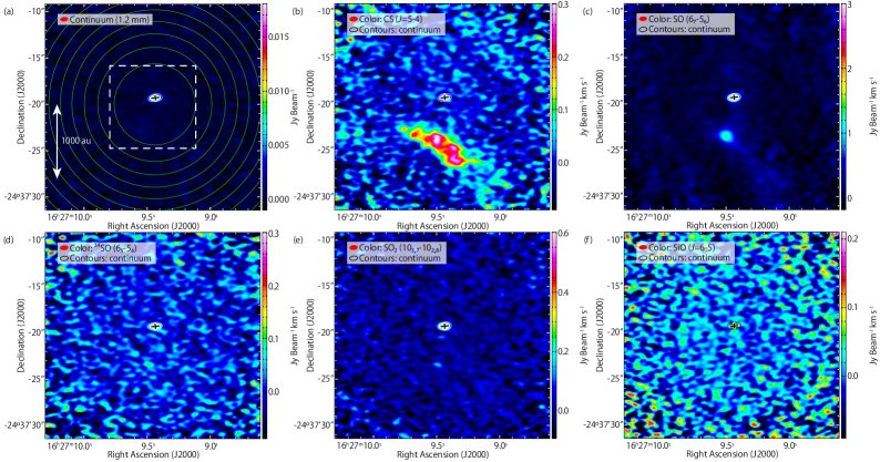
Figure 1: (a) Dust continuum emission at 1.2 mm (254.6 GHz). Integrated intensity maps of the (b) CS ($J=5-4$), (c) SO ($6_{7}-5_{6}$), (d) ³⁴SO ($6_{5}-5_{4}$), (e) SO₂ ($10_{3,7}-10_{2,8}$), and (f) SiO ($J=6-5$) emissions. The velocity range for the integration is $-20$ to 30 km s^-1. White and black contours in each panel represent the continuum map, and the contour levels are at intervals of 10$\sigma$ starting from 10$\sigma$, where the rms level is 0.3 mJy beam^-1. The black cross in each panel represents the continuum peak position, and its size represents the FWHM widths of the image component size convolved with the beam, obtained from two-dimensional Gaussian fitting. The velocity range for integration is $-20$ to $+30$ km s^-1. The images are corrected with the primary beam represented by the green contours in panel (a), whose contour levels are at intervals of 10% starting from 10% of its peak value. The white rectangle in panel (a) represents the area for the blowup maps in Figures 2 and 4.

Images were obtained with the CLEAN algorithm using Briggs weighting with a robust parameter of 0.5. A 1.2 mm continuum image was obtained by averaging line-free channels. The line maps were obtained after subtracting the continuum component directly from the visibility data by resampling to make the channel width 0.5 km s^-1 for ³⁴SO and SiO or 0.1 km s^-1 for the other molecular transitions. The synthesized beam sizes for the spectral lines are listed in Table 1. The root-mean-square (rms) noise level was 0.3 mJy beam^-1 for the continuum and 7, 7, 4, 6, and 4 mJy beam^-1 for CS, SO, ³⁴SO, SO₂, and SiO, respectively, for the channel width mentioned above. A primary beam correction was applied for the continuum and line maps (see Figure 1(a)).

3 Results: Spectral Distribution

3.1 1.2 mm Continuum Emission

Figure 1(a) shows the continuum emission at 1.2 mm. The storing beam is $0\farcs 856\times 0\farcs 470$ (P.A. 95.​​°17). The peak position of the continuum emission was determined to be $(\alpha_{2000},\delta_{2000})=(16^{\rm h}27^{\rm m}09\fs 4358\pm 0.0007,-24\arcdeg 37^{\prime}19\farcs 286\pm 0.004)$, by using two-dimensional Gaussian fitting. The image component sizes convolved with and deconvolved from the beam are $(0\farcs 8845\pm 0\farcs 0216)\times(0\farcs 5632\pm 0\farcs 0092)$ ($\sim 120\times 80$ au) (Position Angle (P.A.) $96.\!\!\arcdeg 0\pm 1.\!\!\arcdeg 4$) and $(0\farcs 312\pm 0\farcs 033)\times(0\farcs 220\pm 0\farcs 134)$ ($\sim 40\times 30$ au) (P.A. $177\arcdeg\pm 57\arcdeg$), respectively. Thus, the continuum emission is marginally resolved by the storing beam.

Two-dimensional Gaussian fitting of the continuum emission yields a peak intensity $I(\nu)$ and integrated flux $F(\nu)$ of $(17.2\pm 0.3)$ mJy beam^-1 and $(21.4\pm 0.7)$ mJy, respectively, where the errors represent three standard deviations (3$\sigma$) of the fit. The beam-averaged column density of H₂ ($N$(H₂)) is obtained from the following equation (Ward-Thompson et al., 2000):

$$N({\rm H}_{2})=\dfrac{2\ln 2\cdot c^{2}}{\pi h\kappa_{\nu}mR_{\rm d}}\times\dfrac{F(\nu)}{\nu^{3}\theta_{\rm major}\theta_{\rm minor}}\times\left(\exp\left(\dfrac{h\nu}{kT}\right)-1\right),$$ (1)

where $\kappa_{\nu}$ is the mass absorption coefficient with respect to the dust mass, $m$ is the average mass of a particle in the gas ($3.83\times 10^{-24}$ g), $\nu$ is the frequency, $\theta_{\rm major}$ and $\theta_{\rm minor}$ are the major and minor beam sizes, respectively, $T$ is the dust temperature, and $R_{\rm d}$ is the dust-to-gas mass ratio (0.01). According to Ossenkopf & Henning (1994), $\kappa_{\nu}$ is estimated to be 1.3 cm² g^-1 at a wavelength of 1.2 mm by interpolation. In this study, we chose the dust opacity model appropriate for dense regions ($10^{8}$ cm^-3) with the MRN grain size distributions (Mathis et al., 1977). The resulting $N$(H₂) and gas mass are shown in Table 2. Because Elias 29 is a relatively evolved source, the dust mass opacity at 1.2 mm could be higher than the typical value for young stellar objects owing to a larger dust size. If we assume $\beta=$ 1.0 (Miotello et al., 2014), $\kappa_{\nu}$ is estimated to be $2.5$ cm² g^-1 ($\kappa_{\nu}\times R_{\rm d}=0.1\times\left(\nu/(10^{12}{\rm\ Hz})\right)^{\beta}$; Beckwith et al., 1990), and $N$(H₂) and gas mass would be smaller by a factor of 2. In the following discussion, we use the former results with $\kappa_{\nu}=$ 1.3 cm² g^-1.

Thus, we calculate $N$(H₂) to be $(3.7\pm 0.4)\times 10^{23}$, $(1.7\pm 0.2)\times 10^{23}$, and $(1.1\pm 0.1)\times 10^{23}$ cm^-2 for dust temperatures of 50, 100, and 150 K, respectively (Table 2). Because we do not have accurate information on the dust temperature, we assume a relatively wide range for it. Here, the errors are taken to be 3$\sigma$ for the integrated flux of the continuum emission. The gas mass is calculated to be $(0.5-1.7)\times 10^{-3}$ $M_{\odot}$ for the dust temperature range from 50 to 150 K.

The peak intensity (17.2 mJy beam^-1) corresponds to a brightness temperature of 0.8 K with the storing beam size. When we use the image size deconvolved from the beam to compensate for beam dilution, the brightness temperature is 4.7 K. Rocha & Pilling (2018) reported the distribution of the dust temperature. According to their model, the dust temperature is about 70 K at a distance of 40 au from the protostar. With these values, the beam-averaged optical depth of the dust continuum is estimated to be 0.07.

3.2 Molecular Lines

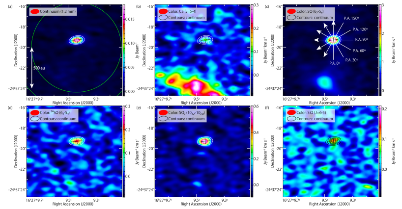
Figure 2: Blowups of Figure 1. (a) Dust continuum emission at 1.2 mm. Integrated intensity maps of the (b) CS, (c) SO, (d) ³⁴SO, (e) SO₂, and (f) SiO emissions. The area for the blowup is represented by the white dashed rectangle in Figure 1(a). See the caption of Figure 1 for details.

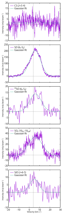
Figure 3: Spectra of the CS, SO, ³⁴SO, SO₂, and SiO lines averaged over a circular region centered at the continuum peak with a diameter of 0$\farcs$5. The green dashed line in each panel shows the result of the Gaussian fitting. The line widths (FWHM) obtained from the Gaussian fitting are $12.7\pm 0.1$, $13.3\pm 1.3$, $15.9\pm 0.6$, and $10.4\pm 1.6$ km s^-1 for the SO, ³⁴SO, SO₂, and SiO lines, respectively, where the central velocities are calculated to be $5.65\pm 0.04$, $6.02\pm 0.45$, $5.76\pm 0.18$, and $4.80\pm 0.61$ km s^-1, respectively.

Figure 1 shows the integrated intensity maps of the CS, SO, ³⁴SO, SO₂, and SiO lines. The velocity range for the integration is $-20$ to 30 km s^-1, where the systemic velocity ($v_{\rm sys}$) is 4.0 km s^-1. Figure 2 shows the blowup of each panel in Figure 1 around the continuum peak, whose area is indicated by the white dashed rectangle in Figure 1(a). Figure 3 shows spectrum of each transition around the continuum peak. The peak integrated intensities of the molecular emission are obtained by using two-dimensional Gaussian fitting to their integrated intensity maps (Table 3).

3.2.1 SO, SO₂, and SiO

The SO, ³⁴SO, SO₂, and SiO emissions show a point source at the continuum peak position. Two-dimensional Gaussian fitting shows the position of the SO intensity peak to be $(\alpha_{2000},\delta_{2000})=(16^{\rm h}27^{\rm m}09\fs 4379\pm 0.0008,-24\arcdeg 37^{\prime}19\farcs 30\pm 0.01)$. The image component sizes (FWHM) of the SO emission convolved with and deconvolved from the beam are $\sim 1\farcs 0\times 0\farcs 7\ (\sim 120\ {\rm au}\times 90\ {\rm au})$ (P.A. $121.\!\!\arcdeg 5\pm 5.\!\!\arcdeg 5$) and $\sim 0\farcs 7\times 0\farcs 3\ (\sim 90\ {\rm au}\times 40\ {\rm au})$ (P.A. $158\arcdeg\pm 11\arcdeg$), respectively.

The intensity ratio ³²SO/³⁴SO is found to be $13\pm 4$ from the peak integrated intensities (Table 3). Because the ³²S/³⁴S ratio in the Solar neighborhood is about 22.6, the ³²SO line is likely optically thick. The optical depth of ³²SO is indeed estimated to be 2.33, including the correction for the different $S\mu^{2}$ values of the two lines. Here, we neglect the small difference in their upper-state energies, because they are close to each other (47.6 and 49.9 K; Table 1).

In determining the column densities and fractional abundances of SO and ³⁴SO relative to H₂, we assume local thermodynamic equilibrium (LTE), as shown in Table 3. We determine the column density and fractional abundance of ³⁴SO by assuming optically thin emission, and determine those of SO from the ³⁴SO results by using ³²S/³⁴S ratio of 22.6.

The SO₂ emission is intense around the protostar, while the SiO emission is marginally detected with a signal-to-noise (S/N) ratio of $\sim 5$ (Figure 2). The column densities and fractional abundances of SO₂ and SiO are calculated under the same assumption as in the ³⁴SO case (Table 3).

The SO emission is also seen on the southeastern side of the continuum peak with an angular offset of about 4″ ($\sim$500 au). This component has an intensity peak position of: $(\alpha_{2000},\delta_{2000})=(16^{\rm h}27^{\rm m}09\fs 489\pm 0.005,-24\arcdeg 37^{\prime}23\farcs 48\pm 0.05)$. Its image component size is $\sim 2\farcs 2\times 1\farcs 5\ (\sim 300\ {\rm au}\times 200\ {\rm au})$. In addition, the ³⁴SO and SO₂ emissions are marginally seen around this position. This component could be due to a local density enhancement (see Section 3.2.2), as previously reported (Lommen et al., 2008). The SO and SO₂ column densities are obtained from their emissions by assuming LTE and optically thin condition (Table 4). We assume a gas temperature of 20 K at this position, according to the dust temperature reported by Rocha & Pilling (2018); the dust temperature is about 25 K at a distance of 500 au from the protostar.

3.2.2 CS

In contrast to the molecular emission described in the previous subsection, the CS emission is weak and marginally detected at the continuum peak position (Figure 2(b)). The faint emission of CS is also confirmed by its spectrum (Figure 3), which shows a weak absorption feature with a narrow line width at a velocity of $\sim$5.5 km s^-1  probably due to foreground gas. The results for column density and fractional abundance of CS toward the continuum peak are listed in Table 3. They might be underestimates owing to the marginal absorption in the red-shifted component. Nevertheless, CS is obviously deficient in the gas near the protostar in comparison with SO.

On the other hand, the CS emission is rather intense in the ridge component on the southeastern side (Figure 1(b)). This component traced by CS extends over 5″ ($\sim$600 au) along the northeast-southwest direction (Figure 1(b)). The CS column density of this component is determined in the same way as for SO and SO₂ (see Section 3.2.1). The results are shown in Table 4.

3.3 Abundance Ratios of the S-bearing Species

Table 4 lists the results for CS, SO, and SO₂ abundance ratios. We have quantitatively confirmed that CS is much less abundant than SO and SO₂ at the continuum peak position. We hereafter assume a gas temperature of 100 K for the continuum peak, based on the dust temperature distribution reported by Rocha & Pilling (2018).

Table 4 also shows previously reported results for comparison: the shocked outflow in L1157 (L1157 B1; Bachiller & Pérez Gutiérrez, 1997), the protostar and the outflow of NGC1333 IRAS 2 (Wakelam et al., 2005), and the envelope gas of the low-mass protostellar source IRAS 16293–2422 Source B (Drozdovskaya et al., 2018). In low-mass protostellar sources, SO is generally thought to be abundant in shocked regions. Indeed, the $N$(SO)/$N$(CS) ratio in L1157 B1 is higher than that in IRAS 16293–2422 Source B by more than one order of magnitude. The results in NGC 1333 IRAS 2 show a large variation in this abundance ratio, which tends to be high in the shocked gas of the eastern outflow lobe (Wakelam et al., 2005). Nevertheless, Elias 29 obviously shows a higher $N$(SO)/$N$(CS) ratio than these sources, although the error is large; the ratio in Elias 29 is higher than that in L1157 B1 by a factor of $\sim$200 and higher than the highest ratio in the shocked gas in NGC 1333 IRAS 2 by a factor of 7.

As shown in Table 4, $N$(SO₂)/$N$(CS) is also higher in the shocked region of L1157 B1 than in IRAS 16293–2422 Source B. As in the case of $N$(SO)/$N$(CS), the $N$(SO₂)/$N$(CS) ratio in Elias 29 is higher than in the other sources by two orders of magnitude.

These results suggest that Elias 29 is significantly richer in SO and SO₂ than in CS. Such a peculiar chemical characteristic is also reported for the low-mass Class I source LFAM 1 (or GSS 30 IRS 3) by Reboussin et al. (2015); that source shows strong emissions of SO, SO₂, and SO⁺. LFAM 1 is also located in the $\rho$ Ophiuchi star-forming region and has strong radio emission at 6 cm (Leous et al., 1991). Reboussin et al. (2015) interpreted their observations as shock chemistry caused by an outflow from this Class I source or from a nearby young stellar object. However, the SO and SO₂ emissions in Elias 29 are clearly associated with the protostar, although we cannot rule out a contribution from the outflow shock near the launching point.

The column densities listed in Table 3 are beam-averaged. As mentioned in Section 3.2, the compact emission concentrated at the continuum peak is only marginally resolved. Thus, the calculated column densities may be underestimates and could be affected by different beam dilutions among the molecules. If the CS emission is more diluted than that of SO or SO₂, the $N$(SO)/$N$(CS) and $N$(SO₂)/$N$(CS) ratios could be overestimated at the CS peak. Observations at higher resolution are required to study such small-scale variation (on size scales of a few 10s of au).

Table 4 also shows the molecular abundances of CS, SO, and SO₂ and their relative abundance ratios in the ridge component of Elias 29. In the ridge, CS seems to be more abundant than at the continuum peak, as shown in Figures 1 and 2. The SO emission is clearly detected in the ridge as well, while the SO₂ emission is marginally detected with a peak intensity of about the 3$\sigma$ confidence level. The $N$(SO)/$N$(CS) and $N$(SO₂)/$N$(CS) ratios are lower than those at the continuum peak by a factor of 5 to 8, although they are still high compared with those of the low-mass protostellar source IRAS 16293–2422 Source B (Drozdovskaya et al., 2018).

4 Chemical Inventory

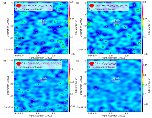
Figure 4: Integrated intensity maps (color) of the (a) HCOOCH₃ ($20_{5,16}$–$19_{5,15}$; E), (b) CH₃OCH₃ ($13_{5,8}$–$13_{4,9}$; EE, AA), (c) CCH ($N$=3–2, $J$=5/2–3/2, $F$=3–2, 2–1), and (d) c-C₃H₂ ($5_{2,3}$–$4_{3,2}$) lines. The velocity range for the integration is 1 to 7 km s^-1. The black cross in each panel represents the continuum peak position and the FWHM widths obtained from two-dimensional Gaussian fitting. The white contours around the cross represent the 1.2 mm dust continuum emission map, where the contour levels are the same as those in Figure 1. The black and grey contours in each panel represent the intensity map of each molecular line. The contour levels are at intervals of 3$\sigma$ starting from 3$\sigma$, where the rms levels are 5, 5, 7, and 9 mJy beam^-1 km s^-1 for the HCOOCH₃, CH₃OCH₃, CCH, and c-C₃H₂ lines, respectively.

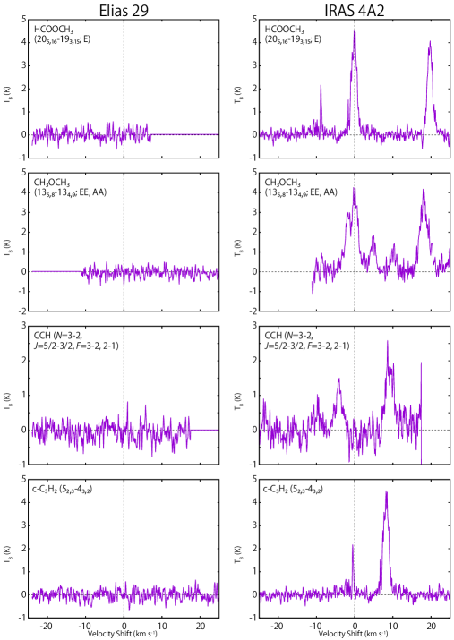
Figure 5: Spectra of the HCOOCH₃, CH₃OCH₃, c-C₃H₂, and CCH lines in Elias 29 and NGC1333 IRAS 4A2 (López-Sepulcre et al., 2017). In Elias 29 (left panels), the spectra are averaged over a circular region centered at the continuum peak with a diameter of 0$\farcs$5, the same as in Figure 3. These observations were performed as a single project to investigate chemical diversity young protostellar sources systematically, and are designed to achieve almost the same sensitivity.

As discussed above, Elias 29 is rich in SO and SO₂, while deficient in CS. Furthermore, Elias 29 is deficient in saturated organic molecules. Figures 4 and 5 show the integrated intensity maps and spectra of the HCOOCH₃ ($20_{5,16}$–$19_{5,15}$; E), CH₃OCH₃ ($13_{5,8}$–$13_{4,9}$; EE, AA), CCH ($N$=3–2, $J$=5/2–3/2, $F$=3–2, 2–1), and c-C₃H₂ ($5_{2,3}$–$4_{3,2}$) lines toward the protostar. These molecular lines are not detected in our observation.

For comparison, Figure 5 shows the spectra observed toward NGC1333 IRAS 4A2 with ALMA (López-Sepulcre et al., 2017). IRAS 4A is a binary system consisting of IRAS 4A1 and IRAS 4A2, where IRAS 4A2 is a hot corino and is chemically richer than IRAS 4A1. In IRAS 4A2, the organic molecular lines HCOOCH₃, CH₃OCH₃, CCH, and c-C₃H₂ are all clearly detected, in contrast with the Elias 29 case, although the observational sensitivity is almost the same for the two sources.

4.1 Deficiency in Organic Molecules

We here derive the upper limits to the column densities of the above molecules. The upper limits to the column densities of HCOOCH₃, CH₃OCH₃, CCH, and c-C₃H₂, are determined from the rms noise levels of their integrated intensity maps in Figure 4, as summarized in Table 5. These upper limits are compared with the corresponding fractional abundances or their upper limits reported for NGC1333 IRAS 4A1 and A2 by López-Sepulcre et al. (2017) (Table 5). the upper limits to the abundances of these molecules in Elias 29 are lower than those in NGC1333 IRAS 4A2 by one order of magnitude, while the constraints for the fractional abundances in Elias 29 are looser than those in NGC 1333 IRAS 4A1.

We here derive the upper limits to the column densities of the above molecules. The rms noise levels of the integrated intensity maps in Figure 4 are 5, 5, 7, and 9 mJy beam^-1 km s^-1 (1$\sigma$) for HCOOCH₃, CH₃OCH₃, CCH, and c-C₃H₂, respectively. Then, the upper limits to the column densities are determined to be $(1.8-2.3)\times 10^{14}$, $(2.9-3.6)\times 10^{14}$, $(4.7-10.1)\times 10^{12}$, and $(3.5-10.4)\times 10^{12}$ cm^-2 for HCOOCH₃, CH₃OCH₃, CCH, and c-C₃H₂, respectively, where we assume LTE and a gas temperature of $(50-150)$ K. These column densities correspond to the fractional-abundance upper limits of $(0.6-2.0)\times 10^{-9}$, $(0.9-3.2)\times 10^{-9}$, $(1.3-9.0)\times 10^{-11}$, and $(0.9-9.2)\times 10^{-11}$, respectively. The fractional abundances of HCOOCH₃ and CH₃OCH₃ in NGC1333 IRAS 4A2 are reported to be $1.1^{+0.2}_{-0.1}\times 10^{-8}$ and $\left(1.0\pm 0.1\right)\times 10^{-8}$ by López-Sepulcre et al. (2017). They also reported the upper limits to these fractional abundances in NGC1333 IRAS 4A1 to be $8.2\times 10^{-11}$ and $4.3\times 10^{-10}$. NGC1333 IRAS 4A1 is the close companion of IRAS 4A2 but is much poorer in molecular line emission. Hence, the upper limits to the abundances of these molecules in Elias 29 are lower than those in NGC1333 IRAS 4A2 by one order of magnitude, while the constraints for the fractional abundances in Elias 29 are looser than those in NGC 1333 IRAS 4A1.

Because the emissions from saturated organic molecules are expected to originate from the hot ($>100$ K) region near the protostar, they could be weak if the hot region is small. This possibility is suggested for NGC1333 IRAS 4A1 (López-Sepulcre et al., 2017). However, this is not the case for Elias 29; according to Boogert et al. (2000), the H₂O gas, which is expected to reside in the hot ($>100$ K) region, was detected in absorption in this source by ISO, with a column density of $\sim 10^{18}$ cm^-2. This corresponds to a high fractional ratio of $10^{-5}$ relative to the total hydrogen column density ($N_{\rm H}\sim 10^{23}$ cm^-2). According to Boogert et al. (2000), Elias 29 should have a hot region where various saturated organic molecules are liberated. They also reported the size of the hot core to be $(85-225)$ au based on observations of infrared absorption of high-$J$ vibration-rotation lines of CO. This size can be resolved in our observation with our beam size $\sim$ 100 au). Furthermore, the dust temperature is above 100 K within $\sim 50$ au of the protostar according to Rocha & Pilling (2018). Therefore, the non-detection of COM lines in our observations is not due to their being frozen-out; instead, it is likely that Elias 29 is very poor in COMs.

The integrated intensity map of the CCH line (Figure 4c) shows a slight negative intensity with a minimum value of $-91$ mJy beam^-1 km s^-1 ($\sim$6$\sigma$) around the protostar, This feature is likely due to self-absorption by foreground gas containing CCH. The extended ambient gas would be resolved-out in this observation with the interferometer, whose maximum recoverable size is $\sim$6″. Nevertheless, no enhancement of the HCOOCH₃, CH₃OCH₃, CCH, or c-C₃H₂ emission is confirmed at least near the protostar, in contrast to the SO and SO₂ cases.

4.2 Possible Cause for the Chemical Characteristics of Elias 29

As described above, one of the interesting chemical features of Elias 29 is its deficiency of organic molecules as well as its richness in SO and SO₂. Here we discuss the following two possibilities: an evolutionary effect after the protostellar birth and an environmental effect. Distinguishing between these alternatives is left for future study.

Elias 29 is a Class I protostar with a bolometric temperature of 391 K (Miotello et al., 2014). Hence, the disk component would have already experienced a temperature above that corresponding to the sublimation of COMS, given the age of this protostar ($(1-5)\times 10^{5}$ yr after the onset of gravitational collapse; Chen et al., 1995). After sublimation, COMs are destroyed by proton transfer reactions with HCO⁺, H₃O⁺, and other ions followed by electron recombination reactions. According to the hot-core model proposed by Nomura & Millar (2004), the time scale for the destruction is about $10^{5}$ yr, which is comparable to the age of the Elias 29 protostar. In this case, the organic molecules liberated from dust grains at the birth of the protostar would have already been broken up by gas reactions. If most of the infalling envelope has already dissipated, fresh grains with COM-ice are no longer supplied. In this case, COMs would be deficient near the protostar. As for the sulfur-bearing molecules, SO and SO₂ can be abundant while CS can be deficient in the gas of an evolved source. SO and SO₂ are the most abundant sulfur-bearing molecules in the gas when the chemical composition of the gas is in a steady state. Thus, the relative maturity of Elias 29 can explain its chemical characteristics. To test this hypothesis, it is necessary to observe other evolved protostellar sources at high spatial resolution and to confirm the dissipation of the envelope gas, which is resolved out in the present observation.

Alternatively, both the deficiency of organic molecules and the richness in SO and SO₂ in Elias 29 could be attributed to the relatively high temperature of the parent core in the starless-core phase due to external heating by nearby objects. These objects include YSOs that are only about 3′ from Elias 29, as well as two bright B stars (S1 and HD147889) (Yui et al., 1993; Ebisawa et al., 2015; Rocha & Pilling, 2018). As mentioned in Section 1, a warm parent core is consistent with the infrared observations of CO and CO₂ (Boogert et al., 2000). It is generally thought that saturated organic molecules, such as CH₃OH and HCOOCH₃, are produced on dust grains by hydrogenation of CO and liberated into the gas near the protostar. It has also been proposed that saturated organic molecules are produced in the gas from CH₃OH liberated from dust grains (Balucani et al., 2015). Meanwhile, it has been suggested that unsaturated carbon-chain molecules and related species, such as CCH and c-C₃H₂, are efficiently produced from methane (CH₄) via sa gas-phase reaction (Sakai & Yamamoto, 2013). CH₄ is the precursor of unsaturated carbon chains and is mainly formed by hydrogenation of atomic carbon on dust grains. Therefore, depletion of either CO or atomic carbon onto dust grains in the prestellar-core stage is required for enhanced production of saturated and unsaturated organic molecules in the protostellar core. Both CO and atomic carbon are depleted onto dust grains with temperatures lower than 20 K (see Appendix A).

As mentioned in Section 1, the dust temperature of the protostellar core Elias 29 is mostly higher than 20 K even on the scale of a few thousand au according to Rocha & Pilling (2018). If the dust temperature were as high as 20 K in the parent cloud of Elias 29 in the past as it is now, CO and atomic carbon would hardly be adsorbed onto dust grains. This may result in insufficient production of the above organic molecules. If this is the case, the deuterium fractionation ratio, which increases after CO depletion onto dust grains, is expected to stay low (e.g. Caselli et al., 2002; Bacmann et al., 2003; Crapsi et al., 2005), although evolutionary effects should also be considered (Imai et al., 2018).

Under the above temperature condition, sulfur atoms will not be depleted onto dust grains either, because the desorption temperature of sulfur atoms is comparable to those of CO and atomic carbon (KIDA; Wakelam et al., 2012, Appendix A). In this case, sulfur atoms are converted to SO and SO₂ through gas-phase reactions (e.g. Prasad & Huntress, 1982; Charnley, 1997; Yoneda et al., 2016; Wakelam et al., 2011). High $N$(SO)/$N$(CS) and $N$(SO₂)/$N$(CS) ratios are expected if the elemental C/O ratio is $>1$, which is plausible considering the detection of water vapor.

Similar chemical characteristics are reported for two other sources: the massive star-forming region G5.89–0.39 and the nearby low-metallicity Large Magellanic Cloud (LMC). G5.89–0.39 consists of shock-heated gas ($150-1800$ K) based on interpretation of CO observations with the SMA tracing the outflows (Su et al., 2012). This source has intense SO and SO₂ line emissions observed by Thompson & MacDonald (1999) with the JCMT and by Hunter et al. (2008) with the SMA. Hunter et al. (2008) also found relatively weak CH₃OH line emission and suggested, as a possible cause, that CO is not well adsorbed onto dust grains. In the high-mass star-forming core ST11 in the LMC, an ALMA observation by Shimonishi et al. (2016) shows bright SO and SO₂ and weak CH₃OH line emissions. While the low metallicity in the LMC (e.g., Dufour et al., 1982) should partly contribute to the low CH₃OH abundance, Shimonishi et al. (2016) suggest that the CH₃OH production is suppressed by warm ice chemistry at the molecular cloud stage. This is supported by a chemical model (Acharyya & Herbst, 2018). We note that CS is less abundant in ST11 than in hot cores in the Milky Way, which is similar to the Elias 29 case. Elias 29 has low mass, while the above sources are massive. However, their similar chemical characteristics could be interpreted in terms of the same scenario with a relatively high dust temperature during the prestellar core phase discussed above.

In this regard, one might conclude that warm core temperatures are common even for high-mass star-forming regions harboring hot cores rich in COMs. However, this does not necessarily contradict the above discussion. A key factor in insufficient COM production on dust surfaces is not the dust temperature at the current protostellar core phase but the temperature during the prestellar phase. Therefore, high-mass star-forming regions rich in COMs can occur if their dust temperature in the prestellar core phase was cold enough for CO depletion and then rose to the current level after the protostellar birth.

5 Rotation Traced by SO

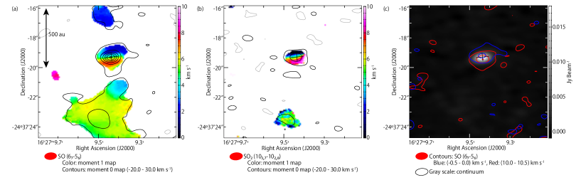
Figure 6: (a) Velocity map of the SO ($6_{7}-5_{6}$) emission (color). The contours represent the integrated intensity map of SO (Figure 2(c)). The contour levels are at intervals of 10$\sigma$ starting from 2$\sigma$, where the rms level is 60 mJy beam^-1. (b) Velocity map of the SO₂ ($10_{3,7}-10_{2,8}$) emission (color). The contours represent the integrated intensity map of SO₂ (Figure 2(e)). The contour levels are at intervals of 10$\sigma$ starting from 2$\sigma$, where the rms level is 30 mJy beam^-1. (c) Integrated intensity maps of the SO emission (contours). The gray scale represents the 1.2 mm continuum map. The velocity ranges for integration are $-0.5$ to 0.0 km s^-1 (blue contours) and 10.0 to 10.5 km s^-1 (red contours). The contour levels are at intervals of 20$\sigma$ starting from 2$\sigma$, where the rms level is 3 mJy beam^-1. The black cross in each panel represents the continuum peak position as in Figure 1.

Figure 6(a) shows the velocity map (the moment 1 map) of the SO ($6_{7}-5_{6}$) line. It reveals a clear velocity gradient along the north-south direction across the continuum peak. This gradient is almost perpendicular to the outflow axis, which was previously reported as running along the east-west direction near the protostar (Ceccarelli et al., 2002). Thus, the gradient most likely represents rotation. Considering its compact distribution, the SO emission seems to trace the disk/envelope system in the vicinity of the protostar. A similar velocity gradient around the protostar is also seen in the SO₂ ($10_{3,7}-10_{2,8}$) emission (Figure 6b). The SO line has a faint blue-shifted component at a distance of 3″ ($\sim 400$ au) north of the protostar, which may come from part of the gas rotating around the protostar. This velocity structure is consistent with the observation of HCO⁺ ($J=3-2$) reported by Lommen et al. (2008). Meanwhile, no clear velocity shift is seen in the SO emission in the ridge component. This component has a large velocity range of $(3-8)$ km s^-1 (a velocity-shift range of $(-1-+4)$ km s^-1 with respect to the systemic velocity of Elias 29), which cannot be attributed to rotation around the protostar. Alternatively, the ridge may come from a gas component in the complex geometrical system surrounding Elias 29 (Boogert et al., 2002).

Figure 6(c) shows the integrated intensity maps of the high velocity-shift components of the SO emission. The velocity ranges for the integration are $-0.5$ to 0.0 km s^-1 and 10.0 to 10.5 km s^-1 for the blue- and red-shifted components, respectively. Two-dimensional Gaussian fitting yields the intensity peak positions $(\alpha_{2000},\delta_{2000})=(16^{\rm h}27^{\rm m}09\fs 4353\pm 0.0011,-24\arcdeg 37^{\prime}19\farcs 145\pm 0.013)$ and $(\alpha_{2000},\delta_{2000})=(16^{\rm h}27^{\rm m}09\fs 4343\pm 0.0008,-24\arcdeg 37^{\prime}19\farcs 419\pm 0.004)$ for the blue- and red-shifted components, respectively. Although the separation ($\sim$0$\farcs$3; $\sim$30 au) is marginal, these peaks are on opposite sides of the continuum peak. Moreover, they align almost on a common line with the P.A. of $\sim$0°. On the basis of this result, we define the P.A. of the mid-plane of the disk/envelope system to be 0°, which means the P.A. of the rotation axis is 270°.

The image component size of the integrated intensity map of the SO line deconvolved from the storing beam is $\sim 0\farcs 7\times 0\farcs 3$ ($\sim 100\times 40$ au) (P.A. $158\arcdeg\pm 11\arcdeg$) (see Section 3.2.1). If we assume a flat disk with no thickness, $i$ is estimated to be 65°. When the thickness of the disk is considered, this value is regarded as the lower limit. This result is in contrast to the inclination angle of less than 60° reported by Boogert et al. (2002) on the basis of a flat spectral energy distribution (SED). However, the analysis of the SED could be affected by gas in the foreground of Elias 29 (e.g. Boogert et al., 2002; Rocha & Pilling, 2018), and thus our result does not seriously conflict with their estimate. For a further constraint, detailed analysis of the outflow will be helpful.

5.1 Kinematic Structure around the Protostar

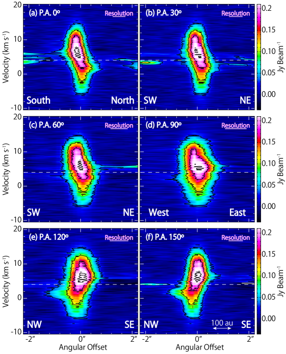
Figure 7: Position-velocity diagrams of the SO ($6_{7}-5_{6}$) line. The position axes are centered at the continuum peak and are along the position angles (a) 0°, (b) 30°, (c) 60°, (d) 90°, (e) 120°, and (f) 150°. The position axis in panel (a) is along the mid-plane of the disk/envelope system. The white dashed lines represent the systemic velocity of 4.0 km s^-1.

Figure 7 shows position-velocity (PV) diagrams of the SO line. The position axes are centered at the continuum peak position. The P.A.s of the position axes are taken for every 30° and are shown in Figure 2(c); Figure 7(a) shows the PV diagram along the mid-plane of the disk/envelope system (P.A. 0°), while Figure 7(d) is along the line perpendicular to it (P.A. 90°).

Figure 7(a) shows a bar-like feature with a clear velocity gradient across the continuum peak; the SO emission is blue- and red-shifted on the northern and southern sides of the continuum peak, respectively. This velocity gradient corresponds to that in Figure 6. The velocity gradient becomes less clear as the P.A. of the position axis increases from 0° to 90°, and it is hardly seen in Figure 7(d) (P.A. 90°). In the PV diagrams with a P.A. greater than 90° (Figures 7(e) and (f)), the velocity gradient is confirmed again; the emissions on the northwestern and southeastern sides of the continuum peak are blue- and red-shifted, respectively. These features are most likely attributed to rotation along the north-south direction without significant infall motion.

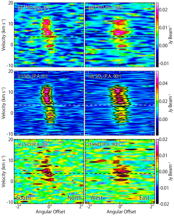
Figure 8: Position-velocity diagrams of the (a, b) ³⁴SO ($6_{5}-5_{4}$), (c, d) SO₂ ($10_{3,7}-10_{2,8}$), and (e, f) DeleteSiO ($J=6-5$) lines. The position axes of panels (a, c, e) are the same as those in panel (a) of Figure 7, and those of panels (b, d, f) are the same as those in panel (d) of Figure 7. The black and white dashed lines represent a systemic velocity of 4.0 km s^-1.

Figure 8 shows the PV diagrams of the ³⁴SO, SO₂, and SiO lines. The S/N ratio is worse for these lines than for the SO line. Nevertheless, the velocity gradient along the north-south direction is as clear in the SO₂ emission (Figure 8c), as in the SO emission. It is difficult to confirm the velocity gradient in the ³⁴SO and SiO emissions because of their insufficient S/N ratios, although a similar velocity-gradient is marginally seen in the SiO emission. Moreover, the red-shifted components look more intense than the blue-shifted components in the SO and SO₂ emissions, and maybe also in the ³⁴SO emission. This is discussed below in Section 5.3.

5.2 Analysis of Rotation

In this section, we discuss the rotation around the protostar found in the SO and SO₂ lines. Because the rotational structure is marginally resolved as shown in Figures 6 and 7, it is difficult to distinguish between Keplerian motion and infall-rotation. Although a clear infall motion is not apparently seen in the PV diagram (Figure 7), we cannot exclude the existence of infall at the current stage. Moreover, the SO and SO₂ spectra do not show the symmetric double-peak characteristic of Keplerian motion (e.g. Eracleous & Halpern, 1994; Dutrey et al., 1997; Öberg et al., 2015; Kastner et al., 2018; Imai et al., 2019), which suggests a contribution from infall. Observations at higher angular resolution are thus necessary to determine the kinematics of the disk/envelope structure, including the disk size and the protostellar mass, accurately. Nonetheless, it is worthwhile to estimate the protostellar mass on the basis of the rotational structure observed in our study. For this purpose, we hereafter assume that the observed rotation is Keplerian, for simplicity.

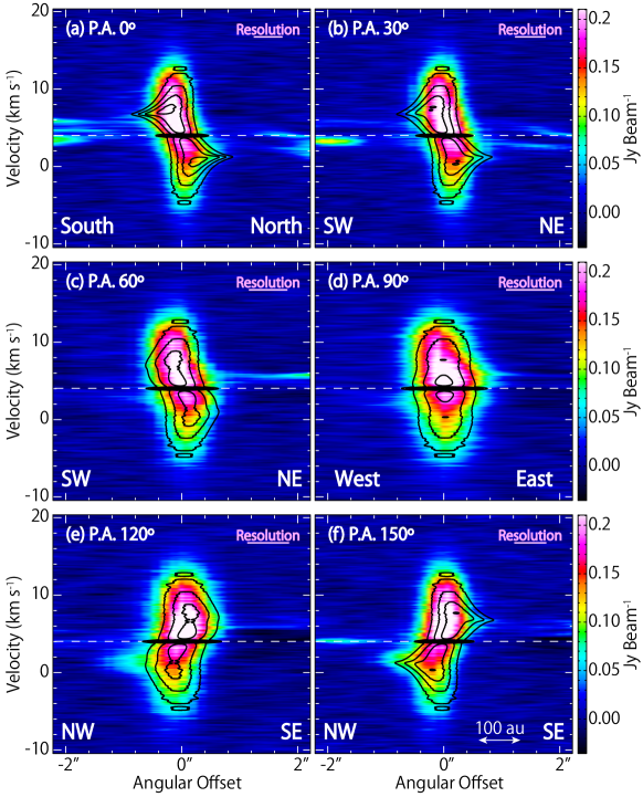
Figure 9: Position-velocity diagrams of the SO ($6_{7}-5_{6}$; color) line in Figure 7 are compared with the result of the Keplerian disk model (black contours). The position axes are the same as those in Figure 7. The white dashed lines represent a systemic velocity of 4.0 km s^-1. We assume a protostellar mass of 1.0 $M_{\odot}$ and inclination angle of 65° (0° for a face-on configuration) for the disk/envelope system. In addition, the emission is assumed to come from the compact region around the protostar with a radius of 100 au. The contour levels for the Keplerian disk model are at intervals of 5% starting from 5% of the peak intensity.

Figure 9 shows the PV diagrams simulated by using the Keplerian disk model (contours); the simulated diagrams are superposed on those of the observed SO emission (color). We use a proportionality coefficient of $r^{-2.0}$ for the emissivity, including the effects of the molecular abundance and temperature profiles, where $r$ denotes the distance from the protostar. In this model, we ignore radiative transfer for simplicity. Thus, the simulated intensity distribution is not accurate enough for detailed comparison with the observation owing to systematic errors. Nevertheless, this simplified model is useful, as found for other sources (e.g. Oya et al., 2017; Okoda et al., 2018), if we focus on the velocity profiles in the comparison. The emission in the model is convolved with the storing beam in the observed SO line.

In Figure 9, the following parameters are used for the Keplerian disk model: the protostellar mass is 1.0 $M_{\odot}$, the inclination angle of the disk/envelope system is 65° (0° for a face-on configuration), and the mid-plane of the disk is extended along a P.A. of 0°. The emission is assumed to come from the compact region around the protostar with a radius of 100 au. This model seems to roughly explain the observed velocity structure, namely, the velocity gradient in the PV diagrams of the SO line. When the inclination angle $i$ is considered explicitly, the protostellar mass is given by

$$M={0.82}\ M_{\odot}\times\dfrac{1}{\sin^{2}i},$$ (2)

where $i=$ 0 for a face-on configuration. For instance, the upper limit of $M$ could be 1.0 $M_{\odot}$ for the lower limit of $i$ (65°; Section 5), while the lower limit could be 0.82 $M_{\odot}$ for the completely edge-on case ($i=90$°). Although these values are not contradict with the lower limit of 0.62 $M_{\odot}$ reported by Lommen et al. (2008) on the basis of their 1.1 mm SMA data of the HCO⁺ ($J=3-2$) line at a resolution of $4\farcs 0\times 2\farcs 3$, assuming the edge-on configuration, the values are lower than those previously employed by a factor of a few; for example, Lommen et al. (2008) reported $2.5\pm 0.6$ $M_{\odot}$ for an inclination angle of 30°, whereas Miotello et al. (2014) reported 3 $M_{\odot}$ using a continuum model. Our result is based on the kinematic structure observed at much higher angular resolution than in the previous studies and provides a better estimate. If the protostellar mass is as small as $\leq 1.0$ $M_{\odot}$, the protostellar age (a few $10^{5}$ yr; Lommen et al., 2008) would be estimated to be younger by a factor of a few. The discrepancy between previous studies and ours is mainly due to the different inclination angle assumed. Indeed, the protostellar mass could be calculated to be 3.3 $M_{\odot}$ with the equation (2), if the inclination angle is 30° as assumed by Lommen et al. (2008). A tighter constraint on the protostellar mass and the inclination angle would require higher angular resolution.

We note that our estimate of the protostellar mass can vary by a factor of a few when we consider possible infall motion. For instance, if we used the infalling-rotating envelope, the protostellar mass would be half of that estimated above via the pure Keplerian model (See Appendix B).

5.3 Asymmetric Spectral Line Profiles of the SO₂ emission

In Figure 3, the SO, SO₂, and SiO lines show a large velocity width over 20 km s^-1. The high-velocity components likely come from the rotating gas in the vicinity of the protostar. The shapes of the spectral profiles are different from one another; the SO and SiO emissions each have a single peak near the systemic velocity ($v_{\rm sys}$ $\sim$ 4.0 km s^-1), while the SO₂ emission is flatter over a velocity shift of 5 km s^-1.

The spectral profile of the SO₂ emission is asymmetric with respect to the systemic velocity (Figure 3). More specifically, the red-shifted part is brighter than the blue-shifted component. This is confirmed in the PV diagrams (Figure 8), as discussed in Section 5.1. Two-dimensional Gaussian fitting of the integrated intensity maps of SO₂ yields blue- and red-shifted peaks of $329\pm 10$ and $225\pm 9$ mJy beam^-1  with integration over the velocity-shift ranges $-4$ to $+4$ km s^-1 and $+4$ to $+12$ km s^-1, respectively, the difference being a factor of 0.68.

A similar asymmetry has been reported for the Class 0 low-mass protostellar source L483 on a scale of 100 au (CS, SO, HNCO, NH₂CHO, HCOOCH₃; Oya et al., 2017). It is suggested that this is due to the asymmetric distribution of these molecules, which could be the case for SO₂ in Elias 29 as well. We note, however, that the line profiles of Elias 29 and L483 are both red-shift deviated, while the asymmetry of a gas distribution should be random, causing either a red-shift or blue-shift deviated profile in principle. In other words, a red-shift deviated line profile could originate from a common physical reason relating to the vicinity of the protostar. We now discuss the following two possibilities.

The weak blue-shifted emission could be explained if the dust in the vicinity of the protostar were optically thick at the corresponding frequency. We consider an edge-on configuration of the disk/envelope system where the molecular gas is infalling. Then, the blue-shifted emission of molecular lines from the back side could be attenuated by dust. The intensity of the blue-shifted emission would be attenuated by a factor of 0.93, if we assumed an optical depth ($\tau$) of 0.07 for the dust (Section 3.1). This attenuation could not explain the observed difference of a factor of 0.68 seen in the SO₂ emission. Here, we note that the above value for $\tau$ is an averaged value around the protostar, and hence, the optical depth of the dust would be higher nearer to the protostar. For a thin disk with a constant density with a radius of $r$ and a scale height of $d$, the optical depth averaged in the circle with a radius of $r$ is smaller than the actual optical depth near the protostar by a factor of $\dfrac{d}{2r}$. This is estimated from the volume between the thin disk and a cylinder with a radius of $r$ and a height of $2r$ surrounding the disk. If the dust continuum emission came from a thin-disk structure with a radius of 20 au and a height of 7 au, $\tau$ would be 0.4. If this were the case and there were infall motion in the vicinity of the protostar, the absorption of the blue-shifted emission by the dust would explain the observed intensity asymmetry in the SO₂ line.

Alternatively, the fact that the blue-shifted emission is weaker than the red-shifted emission could be attributed to expansion. When the gas is expanding, the blue-shifted emission from the gas in front of the protostar is reduced in comparison with the red-shifted emission from the gas to the rear of the protostar (e.g., Beals, 1953). In this case, reduction in intensity occurs mainly for a low-velocity region; this reduction is due to the foreground molecular gas, which has an excitation temperature lower than that of the gas near the protostar. This could be the case in Elias 29 and L483 if the above molecular lines come from the gas in an outflow or a disk wind near the protostar. However, we note that the intensity of the high-velocity region ($v_{\rm shift}\sim-8$ km s^-1) seems to be reduced in Elias 29, which is difficult to attribute to gas in the foreground of the expanding flow. Nevertheless, the possibility that the asymmetry of the intensity due to an outflow or disk wind cannot be excluded at this stage and should be further tested.

6 Summary

We have analyzed ALMA Cycle 2 data obtained for various molecular lines (Table 1) from the Class I protostellar source Elias 29. The major findings are summarized below:

1. The SO and SO₂ lines are bright in the compact region around the protostar within a region of diameter of a few 10s of au. The SO line also traces a ridge component at a distance of 4″ ($\sim$500 au) from the protostar toward the south. SiO emission is detected around the protostar. Meanwhile, the CS emission is weak at the protostar, while it traces the southern ridge component. Around the protostar, the abundance ratio SO/CS is as high as $3^{+13}_{-2}\times 10^{2}$, which is even higher than that found in an outflow shocked region (L1157 B1).

2. Elias 29 is deficient in both saturated and unsaturated organic molecules, such as HCOOCH₃, CH₃OCH₃, CCH, and c-C₃H₂. Their deficiency as well as the richness in SO and SO₂ can be explained qualitatively by chemical evolution of a Class I source or by the relatively high dust temperature ($\>\stackrel{{\scriptstyle\textstyle>}}{{\sim}}\>$20 K) in the parent cloud of Elias 29 in its prestellar core phase. Determining which of these two possibilities applies here is left for future study.

3. The SO and SO₂ emissions show a velocity gradient along the north-south direction across the protostar. Although the gradient is likely due to rotation around the protostar, it is difficult to distinguish between Keplerian motion and infall-rotation in our observation. If we assume this rotation to be Keplerian for simplicity, the kinematic structure that we observed with the SO line can be reproduced by a protostellar mass between 0.82 and 1.0 $M_{\odot}$ by assuming an inclination angle of 90° to 65° (0° for a face-on configuration).

4. The SO₂ spectrum is asymmetric, with the blue-shifted components weaker than the red-shifted. Although this asymmetry can be attributed to an inhomogeneous molecular distribution, we need to consider other possible causes, such as dust opacity or outflow motion.

Appendix A Desorption Temperature

The desorption temperature of a molecular species (also called sublimation temperature) is the typical temperature at which the species thermally desorbs from dust grains. According to Yamamoto (2017), the desorption temperature ($T_{\rm des}$) can be represented in terms of the balance between desorption and adsorption as:

$$k_{\rm B}T_{\rm des} =E_{\rm des}\left(\log\frac{\nu_{0}}{n_{0}\Sigma<v>}\right)^{-1},$$ (A1)

where $E_{\rm des}$ denotes the desorption energy (or binding energy) of molecule X, $\nu_{0}$ the characteristic frequency of the vibration mode, $n_{0}$ the number density of H nuclei, $\Sigma$ the effective collision area of dust per H molecule, and $<v>$ the average speed of X. Typical values for $\nu_{0}$ and $\Sigma$ are $10^{12}$ Hz and $10^{-22}\ {\rm cm}^{2}$, respectively (Hasegawa et al., 1992; Yamamoto, 2017).

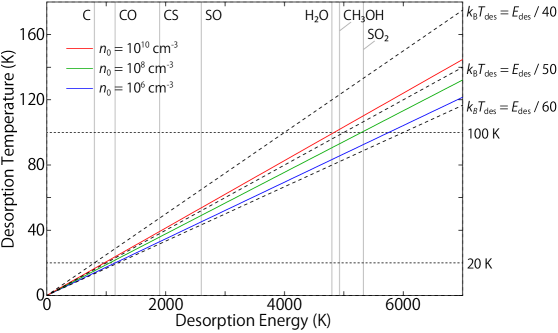
Figure 10: Relation between the desorption temperature and desorption energy. The solid lines represent the plots derived from Equation (A1), where $n_{0}$ and $<v>$ are assumed to be $(10^{6}-10^{10})$ cm^-3 and $0.01$ km s^-1, respectively. The dashed lines are plots of $k_{B}T_{\rm des}=CE_{\rm des}$, where $C$ denotes a proportionality factor of ($40-60$).

Here, the desorption temperature of X is proportional to its desorption energy. Figure 10 shows the relation between the desorption temperature and the desorption energy with typical values for $n_{0}$ and $<v>$. From the plots, the proportionality factor of $T_{\rm des}$ to $E_{\rm des}$ is approximately ($50-60$), which weakly depends on $n_{0}$, $\nu_{0}$, $\Sigma$, and $<v>$. Although $T_{\rm des}$ tends to be higher for higher $n_{0}$, this proportionality relation is practically useful for estimating $T_{\rm des}$. By assuming the factor to be 55 ($n_{0}$ of $10^{8}$ cm^-2 and $<v>$ of 0.1 km s^-1), we can estimate the desorption temperatures of the molecular species in this study as well as some representative molecular species, as summarized in Table 6.

Appendix B Protostellar Mass Estimation with Keplerian Motion and with Combined Infall and Rotation

In Keplerian motion, the rotational velocity ($v_{\rm rot}$) of the gas around the protostar is represented as:

$$v_{\rm rot}(r)=\sqrt{\dfrac{GM}{r}},$$ (B1)

where $M$ denotes the mass of the central protostar and $r$ the radial distance from the protostar. On the other hand, the gas motion can be a combination of infall and rotation. If ballistic motion is assumed, the rotational velocity ($v_{\rm rot}$) and infall velocity ($v_{\rm fall}$) are represented as(Oya et al., 2014):

$$v_{\rm rot}(r) =\dfrac{1}{r}\sqrt{2GMr_{\rm CB}},$$ (B2)

$$v_{\rm fall}(r) =\dfrac{1}{r}\sqrt{2GM(r-r_{\rm CB})},$$ (B3)

where $r_{\rm CB}$ denotes the radius of the centrifugal barrier, which is the perihelion for the infalling gas. At the centrifugal barrier, the gas only rotates, without any radial motion.

When we measure $v_{\rm rot}$ at a certain position at a distance $r$ from the protostar, we can estimate the protostellar mass ($M$) to be $\displaystyle\frac{1}{G}r_{\rm CB}v_{\rm rot}^{2}$ by using equation (B1) for Keplerian motion. For a combination of infall and rotation, we need to specify $r_{\rm CB}$. When we simply assume that the position is the centrifugal barrier, the protostellar mass is calculated to be $\dfrac{1}{2G}r_{\rm CB}v_{\rm rot}^{2}$ with Equation (B2). This is half of the mass derived by assuming Keplerian motion.

Table 1: Parameters of the Observed Lines

Molecule	Transition	Frequency (GHz)	$E_{\rm u}$ (K)	$S\mu^{2}$ (Debye2)	$A_{ij}$ ($s^{-1}$)	Synthesized Beam
Continuum	(1.2 mm)	$244.91-264.26$				$0\farcs 856\times 0\farcs 470$ (P.A. 95.​​°17)
CS	$J=5-4$	244.9355565	35.3	19.2	$2.98\times 10^{-4}$	$0\farcs 884\times 0\farcs 522$ (P.A. 94.​​°60)
SO	$6_{7}-5_{6}$	261.8437210	47.6	16.4	$2.28\times 10^{-4}$	$0\farcs 832\times 0\farcs 488$ (P.A. 94.​​°17)
34SO	$6_{5}-5_{4}$	246.6634700	49.9	11.4	$1.81\times 10^{-4}$	$0\farcs 883\times 0\farcs 517$ (P.A. 94.​​°64)
SO2	$10_{3,7}-10_{2,8}$	245.5634219	72.7	14.5	$1.19\times 10^{-4}$	$0\farcs 885\times 0\farcs 520$ (P.A. 94.​​°78)
SiO	$J=6-5$	260.5180090	43.8	57.6	$9.12\times 10^{-4}$	$0\farcs 835\times 0\farcs 488$ (P.A. 94.​​°67)

Table 2: 1.2 mm Dust Continuum Parameters

Peak Intensity	Integrated Flux	Assumed	$M_{\rm gas}$	$n$(H2)
$I(\nu)$ (mJy beam-1)	$F(\nu)$ (mJy)	Dust Temperature	($10^{-3}$ $M_{\odot}$)	($10^{23}$ cm-2)
$17.2\pm 0.3$	$21.4\pm 0.7$	50 K	$1.68\pm 0.06$	$3.7\pm 0.4$
		100 K	$0.79\pm 0.03$	$1.7\pm 0.2$
		150 K	$0.52\pm 0.02$	$1.1\pm 0.1$

Table 3: Observed Intensities and Derived Abundances at the Continuum Peak

Species	$I(\nu)$	Assumed	Column Density	Fractional Abundance
	(Jy beam-1 km s-1)	Gas Temperature	$N(X)$ (cm-2)	$f(X)$
CS	$0.116\pm 0.03$	50 K	$(1.6\pm 1.2)\times 10^{13}$	$(4.2\pm 3.3)\times 10^{-11}$
		100 K	$(2.2\pm 1.7)\times 10^{13}$	$(1.3\pm 1.0)\times 10^{-10}$
		150 K	$(2.9\pm 2.3)\times 10^{13}$	$(2.6\pm 2.0)\times 10^{-10}$
SO	$2.83\pm 0.33$	50 K	$(4.6\pm 1.4)\times 10^{15}$	$(1.3\pm 0.4)\times 10^{-8}$
		100 K	$(6.0\pm 1.8)\times 10^{15}$	$(3.5\pm 1.0)\times 10^{-8}$
		150 K	$(7.8\pm 2.3)\times 10^{15}$	$(6.9\pm 2.0)\times 10^{-8}$
34SO	$0.225\pm 0.0966$	50 K	$(2.0\pm 0.6)\times 10^{14}$	$(5.6\pm 1.6)\times 10^{-10}$
		100 K	$(2.7\pm 0.8)\times 10^{14}$	$(1.5\pm 0.5)\times 10^{-9}$
		150 K	$(3.5\pm 1.0)\times 10^{14}$	$(3.1\pm 0.9)\times 10^{-9}$
SO2	$0.621\pm 0.052$	50 K	$(2.2\pm 0.6)\times 10^{15}$	$(6.0\pm 1.5)\times 10^{-9}$
		100 K	$(3.0\pm 0.8)\times 10^{15}$	$(1.7\pm 0.4)\times 10^{-8}$
		150 K	$(4.4\pm 1.1)\times 10^{15}$	$(3.9\pm 1.0)\times 10^{-8}$
SiO	$0.113\pm 0.024$	50 K	$(6.4\pm 4.1)\times 10^{12}$	$(1.7\pm 1.1)\times 10^{-11}$
		100 K	$(8.3\pm 5.3)\times 10^{12}$	$(4.8\pm 3.0)\times 10^{-11}$
		150 K	$(1.1\pm 0.7)\times 10^{13}$	$(9.5\pm 6.0)\times 10^{-11}$

Table 4: Column Densities and Abundance Ratios of Sulfur-Bearing Species Compared with Other Sources

	Elias 29	Elias 29	NGC 1333 IRAS 2	IRAS 16293–2422	L1157 B1
	Continuum Peak	Ridge		Source B
$N$(CS) /cm-2	$(2.2\pm 1.7)\times 10^{13}$	$(5.1\pm 1.4)\times 10^{13}$	$(0.5-4.5)\times 10^{13}$	$(4.4-66)\times 10^{15}$	$2.7\times 10^{14}$
$N$(SO) /cm-2	$(6.0\pm 1.8)\times 10^{15}$	$(9.8\pm 2.6)\times 10^{14}$	$(0.6-3.5)\times 10^{14}$	$<5.0\times 10^{14}$	$(3-5)\times 10^{14}$
$N$(SO2) /cm-2	$(3.0\pm 0.8)\times 10^{15}$	$(1.3\pm 1.2)\times 10^{15}$	$(0.5-7.0)\times 10^{13}$	$1.5\times 10^{15}$	$3.0\times 10^{14}$
$N$(SO)/$N$(CS)	$3^{+13}_{-2}\times 10^{2}$	$19^{+14}_{-8}$	$1.7-37.5$	$<0.11$	$1.1-1.9$
$N$(SO2)/$N$(CS)	$1.4^{+6}_{-0.8}\times 10^{2}$	$25^{+43}_{-24}$	$0.1-6.3$	$0.02-0.34$	$1.1$
$N$(SO2)/$N$(SO)	$0.5^{+0.4}_{-0.2}$	$1.3^{+2.2}_{-1.3}$	$0.05-0.3$	$>3$	$0.6-1.0$

Table 5: Abundances of Organic Molecules at the Continuum Peak

Species	Elias 29			NGC1333 IRAS 4A1	NGC1333 IRAS 4A2
	Integrated Intensity	Column Density	$N$($X$)/$N$(H2)	$N$($X$)/$N$(H2)	$N$($X$)/$N$(H2)
HCOOCH3	$<5$	$<(1.8-2.3)\times 10^{14}$	$<(0.6-2.0)\times 10^{-9}$	$<8.2\times 10^{-11}$	$(1.1\pm 0.1)\times 10^{-8}$
CH3OCH3	$<5$	$<(2.9-3.6)\times 10^{14}$	$<(0.9-3.2)\times 10^{-9}$	$<4.3\times 10^{-10}$	$(1.0\pm 0.1)\times 10^{-8}$
CCH	$<7$	$<(4.7-10.1)\times 10^{12}$	$<(1.3-9.0)\times 10^{-11}$
c-C3H2	$<9$	$<(3.5-10.4)\times 10^{12}$	$<(0.9-9.2)\times 10^{-11}$

Table 6: Desorption Energies and Desorption Temperatures of Molecular Species

Molecular Species	Desorption Energy	Desorption Temperature
	$E_{\rm des}$$/k_{B}$ (K)	$T_{\rm des}$(K)
C	800	15
S	1100	20
CO	1150	21
O	1600	30
CS	1900	35
H2CO	2050	37
CCH	2137	39
SO	2600	47
H2CS	2700	49
H2S	2743	50
OCS	2888	53
SiO	3500	64
HCOOCH3	4000	73
H2O	4800	87
CH3OH	4930	90
HCOOH	5000	91
SO2	5330	97
NH2CHO	5556	101

References

- Acharyya & Herbst (2018) Acharyya, K., & Herbst, E. 2018, ApJ, 859, 51
- Bachiller & Pérez Gutiérrez (1997) Bachiller, R., & Pérez Gutiérrez, M. 1997, ApJ, 487, L93
- Bacmann et al. (2003) Bacmann, A., Lefloch, B., Ceccarelli, C., et al. 2003, ApJ, 585, L55
- Balucani et al. (2015) Balucani, N., Ceccarelli, C., & Taquet, V. 2015, MNRAS, 449, L16
- Beals (1953) Beals, C. S. 1953, Publications of the Dominion Astrophysical Observatory Victoria, 9, 1
- Beckwith et al. (1990) Beckwith, S. V. W., Sargent, A. I., Chini, R. S., & Guesten, R. 1990, AJ, 99, 924
- Bontemps et al. (1996) Bontemps, S., Andre, P., Terebey, S., & Cabrit, S. 1996, A&A, 311, 858
- Boogert et al. (2000) Boogert, A. C. A., Tielens, A. G. G. M., Ceccarelli, C., et al. 2000, A&A, 360, 683
- Boogert et al. (2002) Boogert, A. C. A., Hogerheijde, M. R., Ceccarelli, C., et al. 2002, ApJ, 570, 708
- Bussmann et al. (2007) Bussmann, R. S., Wong, T. W., Hedden, A. S., Kulesa, C. A., & Walker, C. K. 2007, ApJ, 657, L33
- Caselli et al. (2002) Caselli, P., Walmsley, C. M., Zucconi, A., et al. 2002, ApJ, 565, 344
- Ceccarelli et al. (2002) Ceccarelli, C., Boogert, A. C. A., Tielens, A. G. G. M., et al. 2002, A&A, 395, 863
- Charnley (1997) Charnley, S. B. 1997, ApJ, 481, 396
- Chen et al. (1995) Chen, H., Myers, P. C., Ladd, E. F., & Wood, D. O. S. 1995, ApJ, 445, 377
- Crapsi et al. (2005) Crapsi, A., Caselli, P., Walmsley, C. M., et al. 2005, ApJ, 619, 379
- Drozdovskaya et al. (2018) Drozdovskaya, M. N., van Dishoeck, E. F., Jørgensen, J. K., et al. 2018, MNRAS, 476, 4949
- Dufour et al. (1982) Dufour, R. J., Shields, G. A., & Talbot, R. J., Jr. 1982, ApJ, 252, 461
- Dutrey et al. (1997) Dutrey, A., Guilloteau, S., & Guelin, M. 1997, A&A, 317, L55
- Ebisawa et al. (2015) Ebisawa, Y., Inokuma, H., Sakai, N., et al. 2015, ApJ, 815, 13
- Elias (1978) Elias, J. H. 1978, ApJ, 224, 453
- Eracleous & Halpern (1994) Eracleous, M., & Halpern, J. P. 1994, ApJS, 90, 1
- Evans et al. (2009) Evans, N. J., II, Dunham, M. M., Jørgensen, J. K., et al. 2009, ApJS, 181, 321
- Favata et al. (2005) Favata, F., Micela, G., Silva, B., Sciortino, S., & Tsujimoto, M. 2005, A&A, 433, 1047
- Giardino et al. (2007) Giardino, G., Favata, F., Pillitteri, I., et al. 2007, A&A, 475, 891
- Gómez et al. (2003) Gómez, M., Stark, D. P., Whitney, B. A., & Churchwell, E. 2003, AJ, 126, 863
- Graninger et al. (2016) Graninger, D. M., Wilkins, O. H., & Öberg, K. I. 2016, ApJ, 819, 140
- Hasegawa et al. (1992) Hasegawa, T. I., Herbst, E., & Leung, C. M. 1992, ApJS, 82, 167
- Higuchi et al. (2018) Higuchi, A. E., Sakai, N., Watanabe, Y., et al. 2018, ApJS, 236, 52
- Hunter et al. (2008) Hunter, T. R., Brogan, C. L., Indebetouw, R., & Cyganowski, C. J. 2008, ApJ, 680, 1271
- Imai et al. (2016) Imai, M., Sakai, N., Oya, Y., et al. 2016, ApJ, 830, L37
- Imai et al. (2018) Imai, M., Sakai, N., López-Sepulcre, A., et al. 2018, ApJ, 869, 51
- Imai et al. (2019) Imai, M., et al., 2019, submitted to ApJ
- Imanishi et al. (2001) Imanishi, K., Koyama, K., & Tsuboi, Y. 2001, ApJ, 557, 747
- Jørgensen et al. (2009) Jørgensen, J. K., van Dishoeck, E. F., Visser, R., et al. 2009, A&A, 507, 861
- Kastner et al. (2018) Kastner, J. H., Qi, C., Dickson-Vandervelde, D. A., et al. 2018, ApJ, 863, 106
- Lee et al. (2017) Lee, C.-F., Li, Z.-Y., Ho, P. T. P., et al. 2017, ApJ, 843, 27
- Lefloch et al. (2018) Lefloch, B., Bachiller, R., Ceccarelli, C., et al. 2018, MNRAS, 477, 4792
- Leous et al. (1991) Leous, J. A., Feigelson, E. D., Andre, P., & Montmerle, T. 1991, ApJ, 379, 683
- Lindberg & Jørgensen (2012) Lindberg, J. E., & Jørgensen, J. K. 2012, A&A, 548, A24
- Lindberg et al. (2016) Lindberg, J. E., Charnley, S. B., & Cordiner, M. A. 2016, ApJ, 833, L14
- Liseau et al. (1999) Liseau, R., White, G. J., Larsson, B., et al. 1999, A&A, 344, 342
- Lommen et al. (2008) Lommen, D., Jørgensen, J. K., van Dishoeck, E. F., & Crapsi, A. 2008, A&A, 481, 141
- López-Sepulcre et al. (2017) López-Sepulcre, A., Sakai, N., Neri, R., et al. 2017, A&A, 606, A121
- Lundgren (2013) Lundgren, A., 2013, ALMA Cycle 2 Technical Handbook Version 1.1, ALMA
- Mathis et al. (1977) Mathis, J. S., Rumpl, W., & Nordsieck, K. H. 1977, ApJ, 217, 425
- Millar et al. (1991) Millar, T. J., Herbst, E., & Charnley, S. B. 1991, ApJ, 369, 147
- Miotello et al. (2014) Miotello, A., Testi, L., Lodato, G., et al. 2014, A&A, 567, A32
- Müller et al. (2005) Müller, H. S. P., Schlöder, F., Stutzki, J., & Winnewisser, G. 2005, Journal of Molecular Structure, 742, 215
- Nakamura et al. (2011) Nakamura, F., Kamada, Y., Kamazaki, T., et al. 2011, ApJ, 726, 46
- Nomura & Millar (2004) Nomura, H., & Millar, T. J. 2004, A&A, 414, 409
- Öberg et al. (2015) Öberg, K. I., Guzmán, V. V., Furuya, K., et al. 2015, Nature, 520, 198
- Okoda et al. (2018) Okoda, Y., Oya, Y., Sakai, N., et al. 2018, ApJ, 864, L25
- Ortiz-León et al. (2017) Ortiz-León, G. N., Loinard, L., Kounkel, M. A., et al. 2017, ApJ, 834, 141
- Ossenkopf & Henning (1994) Ossenkopf, V., & Henning, T. 1994, A&A, 291, 943
- Oya et al. (2014) Oya, Y., Sakai, N., Sakai, T., et al. 2014, ApJ, 795, 152
- Oya et al. (2016) Oya, Y., Sakai, N., López-Sepulcre, A., et al. 2016, ApJ, 824, 88
- Oya et al. (2017) Oya, Y., Sakai, N., López-Sepulcre, A., et al. 2017, ApJ, 837, 174
- Prasad & Huntress (1982) Prasad, S. S., & Huntress, W. T., Jr. 1982, ApJ, 260, 590
- Reboussin et al. (2015) Reboussin, L., Guilloteau, S., Simon, M., et al. 2015, A&A, 578, A31
- Rocha & Pilling (2015) Rocha, W. R. M., & Pilling, S. 2015, ApJ, 803, 18
- Rocha & Pilling (2018) Rocha, W. R. M., & Pilling, S. 2018, MNRAS, 478, 5190
- Sakai et al. (2008) Sakai, N., Sakai, T., Hirota, T., & Yamamoto, S. 2008a, ApJ, 672, 371
- Sakai & Yamamoto (2013) Sakai, N., & Yamamoto, S. 2013, Chemical Reviews, 113, 8981
- Sakai et al. (2016) Sakai, N., Oya, Y., López-Sepulcre, A., et al. 2016, ApJ, 820, L34
- Sekimoto et al. (1997) Sekimoto, Y., Tatematsu, K., Umemoto, T., et al. 1997, ApJ, 489, L63
- Shimonishi et al. (2016) Shimonishi, T., Onaka, T., Kawamura, A., & Aikawa, Y. 2016, ApJ, 827, 72
- Su et al. (2012) Su, Y.-N., Liu, S.-Y., Chen, H.-R., & Tang, Y.-W. 2012, ApJ, 744, L26
- Thompson & MacDonald (1999) Thompson, M. A., & MacDonald, G. H. 1999, A&AS, 135, 531
- van der Marel et al. (2013) van der Marel, N., Kristensen, L. E., Visser, R., et al. 2013, A&A, 556, A76
- van Kempen et al. (2009) van Kempen, T. A., van Dishoeck, E. F., Salter, D. M., et al. 2009, A&A, 498, 167
- Wakelam et al. (2005) Wakelam, V., Ceccarelli, C., Castets, A., et al. 2005, A&A, 437, 149
- Wakelam et al. (2011) Wakelam, V., Hersant, F., & Herpin, F. 2011, A&A, 529, A112
- Wakelam et al. (2012) Wakelam, V., Herbst, E., Loison, J.-C., et al. 2012, ApJS, 199, 21
- Ward-Thompson et al. (2000) Ward-Thompson, D., Zylka, R., Mezger, P. G., & Sievers, A. W. 2000, A&A, 355, 1122
- Wilking & Lada (1983) Wilking, B. A., & Lada, C. J. 1983, ApJ, 274, 698
- Yamamoto (2017) Yamamoto, S., 2017, ‘Introduction to Astrochemistry: Chemical Evolution from Interstellar Clouds to Star and Planet Formation’, Springer, (Berlin, Heidelberg)
- Ybarra et al. (2006) Ybarra, J. E., Barsony, M., Haisch, K. E., Jr., et al. 2006, ApJ, 647, L159
- Yoneda et al. (2016) Yoneda, H., Tsukamoto, Y., Furuya, K., & Aikawa, Y. 2016, ApJ, 833, 105
- Yui et al. (1993) Yui, Y. Y., Nakagawa, T., Doi, Y., et al. 1993, ApJ, 419, L37